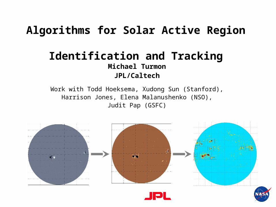
Algorithms for Solar Active Region Identification and Tracking

Michael TurmonJPL/Caltech

Work with Todd Hoeksema, Xudong Sun (Stanford),Harrison Jones, Elena Malanushenko (NSO),

Judit Pap (GSFC)

2

Capabilities Discussed Here

Identification– Label active pixels in multivariate images, e.g.: (LOS B, Ic)– There exists a family of methods by many researchers– Largely a solved problem for active regions in photosphere– Bayesian approach maximizing posterior probability of labeling

• Has been released for HMI on jsoc.stanford.edu

Tracking– Grouping of active pixels in labeling into ARs– Then, link identified ARs through a series of images– Single-link most likely tracker (optimization-based association)– Nearing release for HMI as hmi.Mharp_720s

Motivation

• Identification: Find objects in multispectral images

• Tracking: Link identified objects across a series of images

• Object Analysis: Model and classify object tracks

Move beyond looking at pixels to understanding phenomena

Identification

Allow scientists in to understand great volumes of spatio-temporal data in directly informative terms

Tracking Object analysis

4

Identification

5

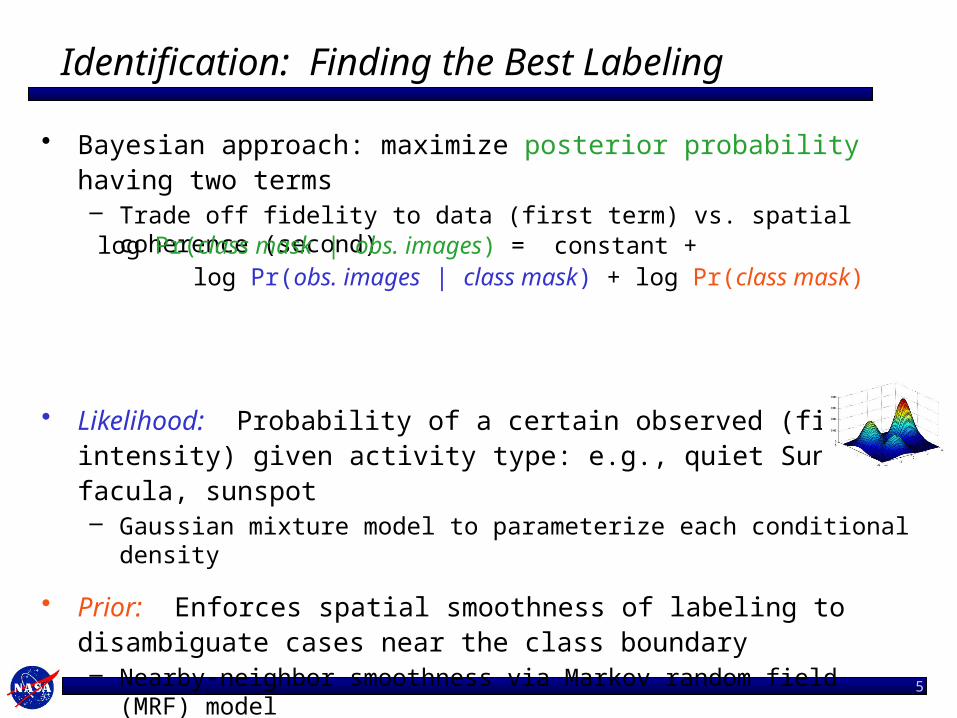
Identification: Finding the Best Labeling

• Bayesian approach: maximize posterior probability having two terms– Trade off fidelity to data (first term) vs. spatial coherence (second)

• Likelihood: Probability of a certain observed (field, intensity) given activity type: e.g., quiet Sun, facula, sunspot– Gaussian mixture model to parameterize each conditional density

• Prior: Enforces spatial smoothness of labeling to disambiguate cases near the class boundary– Nearby-neighbor smoothness via Markov random field (MRF) model

• Find mask via discrete optimization of posterior w.r.t. entire labeling

log Pr(class mask | obs. images) = constant + log Pr(obs. images | class mask) + log Pr(class mask)

6

Photogram

Magnetogram

SNQ

Key:S(pot)F(acula)Q(uiet sun)

S

FQ

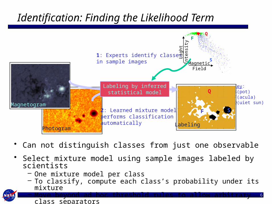
1: Experts identify classesin sample images

2: Learned mixture model performs classification automatically

MagneticField

Light

Intensity

Labeling

Labeling by inferredstatistical model Q

SF

Identification: Finding the Likelihood Term

• Can not distinguish classes from just one observable

• Select mixture model using sample images labeled by scientists– One mixture model per class– To classify, compute each class’s probability under its mixture– Move beyond ad hoc threshold rules to allow arbitrary class separators

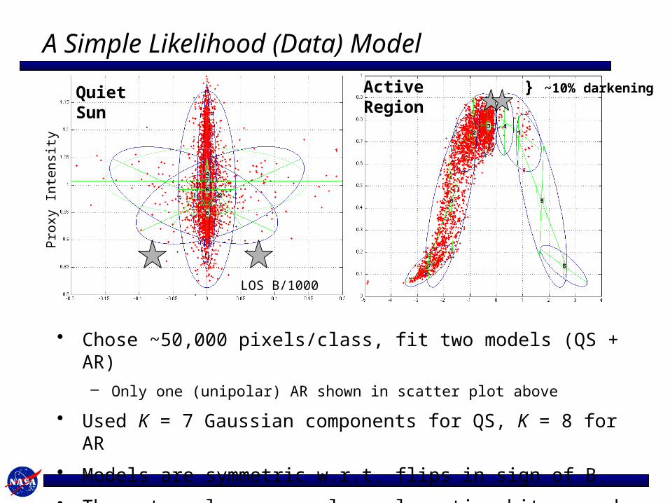
A Simple Likelihood (Data) Model

• Chose ~50,000 pixels/class, fit two models (QS + AR)– Only one (unipolar) AR shown in scatter plot above

• Used K = 7 Gaussian components for QS, K = 8 for AR

• Models are symmetric w.r.t. flips in sign of B

• These two classes overlap only a tiny bit around the stars

QuietSun

Active Region

LOS B/1000

Pro

xy I

nte

nsi

ty

} ~10% darkening

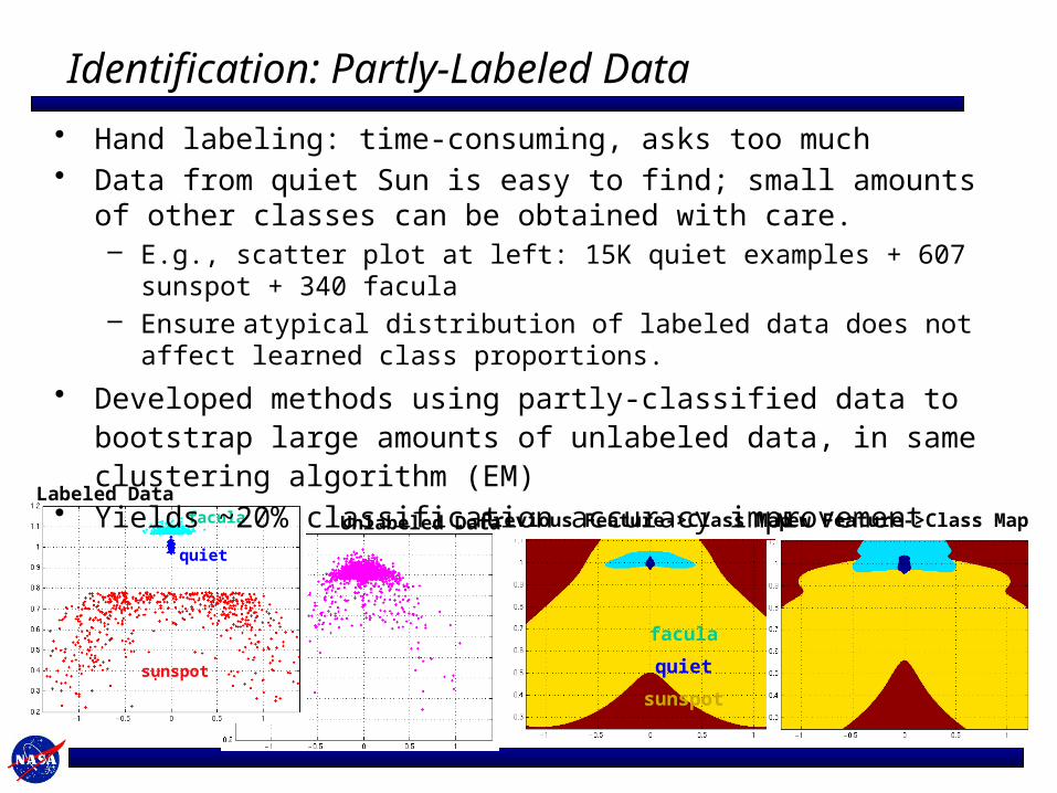
Unlabeled Data

Labeled Data

sunspot

quiet

facula

facula

quiet

sunspot

Previous Feature->Class Map New Feature->Class Map

Identification: Partly-Labeled Data

• Hand labeling: time-consuming, asks too much• Data from quiet Sun is easy to find; small amounts of other classes can

be obtained with care.– E.g., scatter plot at left: 15K quiet examples + 607 sunspot + 340 facula– Ensure atypical distribution of labeled data does not affect learned class

proportions.

• Developed methods using partly-classified data to bootstrap large amounts of unlabeled data, in same clustering algorithm (EM)

• Yields ~20% classification accuracy improvement

9

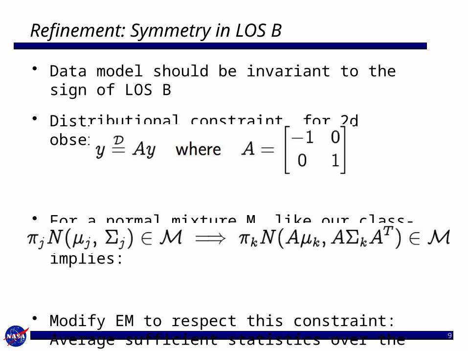
• Data model should be invariant to the sign of LOS B

• Distributional constraint, for 2d observation y:

• For a normal mixture M, like our class-conditional likelihoods, the constraint implies:

• Modify EM to respect this constraint: Average sufficient statistics over the cyclic groups associated with A.

Refinement: Symmetry in LOS B

10

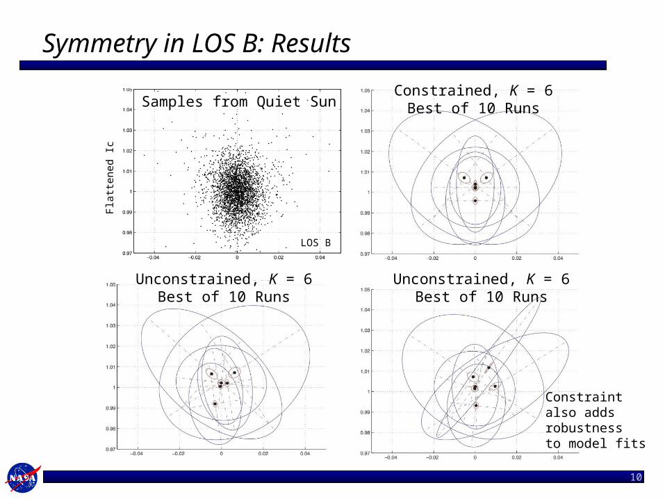
Symmetry in LOS B: Results

Constraintalso addsrobustnessto model fits

Constrained, K = 6Best of 10 Runs

Unconstrained, K = 6Best of 10 Runs

Unconstrained, K = 6Best of 10 Runs

LOS B

Fla

tten

ed I

cSamples from Quiet Sun

11

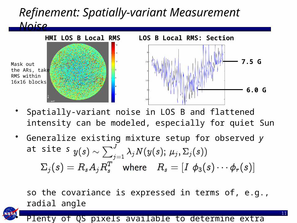
Refinement: Spatially-variant Measurement Noise

• Spatially-variant noise in LOS B and flattened intensity can be modeled, especially for quiet Sun

• Generalize existing mixture setup for observed y at site s:

so the covariance is expressed in terms of, e.g., radial angle

• Plenty of QS pixels available to determine extra parameters in Aj

HMI LOS B Local RMS LOS B Local RMS: Section

Mask outthe ARs, takeRMS within16x16 blocks

7.5 G

6.0 G

12

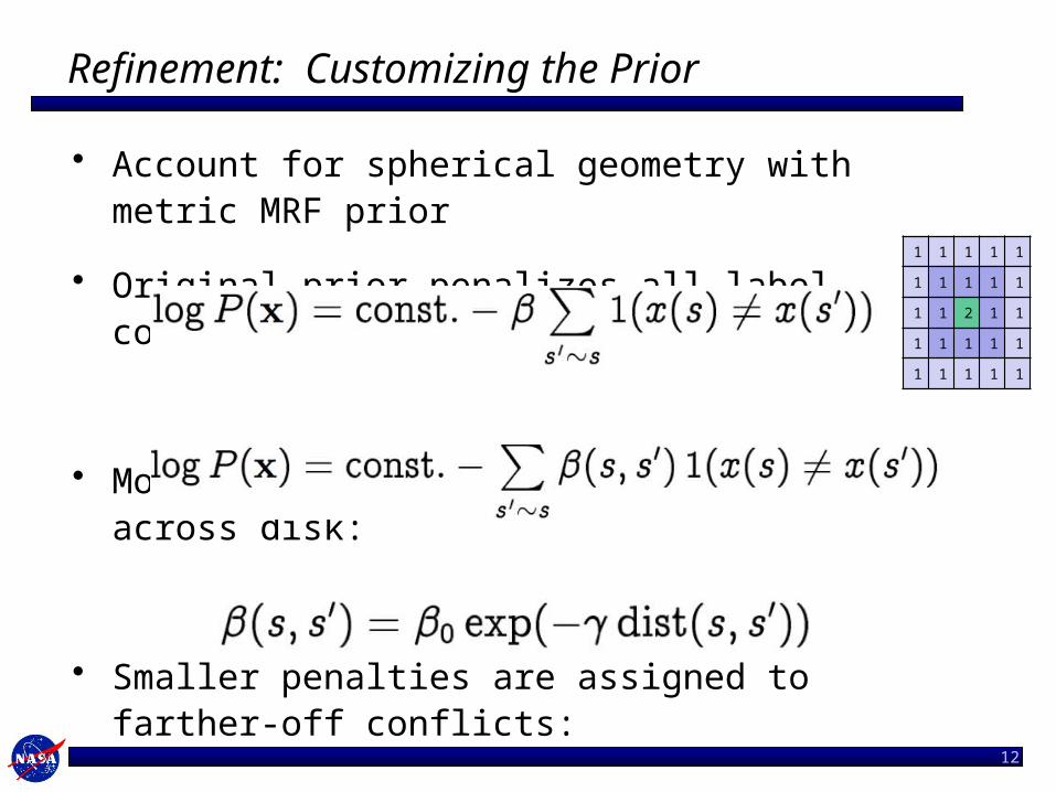
Refinement: Customizing the Prior

• Account for spherical geometry with metric MRF prior

• Original prior penalizes all label-conflicts equally:

• Modified prior penalizes differently across disk:

• Smaller penalties are assigned to farther-off conflicts:

where dist(s, s’) = great-circle distance between sites

1 1 1 1 1

1 1 1 1 1

1 1 2 1 1

1 1 1 1 1

1 1 1 1 1

13

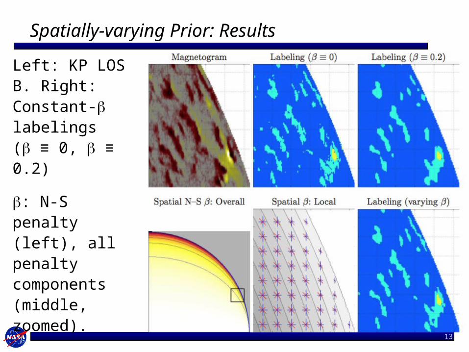
Spatially-varying Prior: Results

Left: KP LOS B. Right: Constant-b labelings(b ≡ 0, b ≡ 0.2)

b: N-S penalty (left), all penalty components (middle, zoomed).

Rightmost: labeling with variable b

14

HMI Identification Status

• Output Masks– Available as hmi.Marmask_720s and hmi.Marmask_720s_nrt– Full-disk 4Kx4K mask images in coordinates of observations– Never re-map observed images to find the mask

• Further Calibration– Calibration team is working on better removal of limb-

darkening and time-dependent flat-field from intensity proxy.– Current HMI region model does not really use the intensity

proxy because of limb artifacts.

• Enhancements– A more detailed class breakdown is possible. – E.g., umbra/penumbra were not reliably determined from MDI;

believe HMI should be better

15

Tracking

16

Components of “Tracking”

• Identification (just discussed)

• Grouping – Group separated features into AR– Formal literature on this is not well-developed– Use a simple template-based method

• Association– Construct 1:1 map from previous AR set to next AR set.

• Chained together, you have a track.– Criterion: maximize cumulative area of overlap– Heuristics to “look harder” for new or dying ARs

• Naming– Link a track to a name like NOAA AR#9077

17

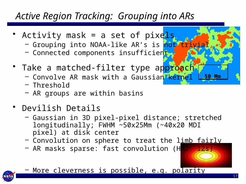
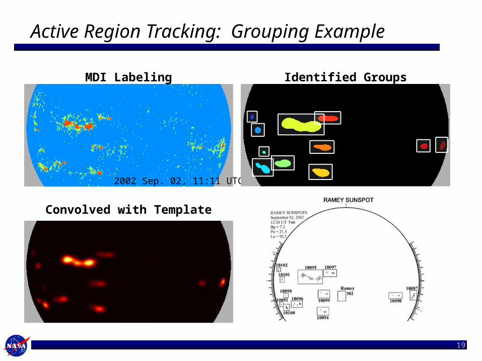
Active Region Tracking: Grouping into ARs

• Activity mask = a set of pixels– Grouping into NOAA-like AR’s is not trivial– Connected components insufficient

• Take a matched-filter type approach– Convolve AR mask with a Gaussian kernel– Threshold– AR groups are within basins

• Devilish Details– Gaussian in 3D pixel-pixel distance; stretched longitudinally;

FWHM ~50x25Mm (~40x20 MDI pixel) at disk center– Convolution on sphere to treat the limb fairly– AR masks sparse: fast convolution (HMI: 12s)

– More cleverness is possible, e.g. polarity

50 Mm

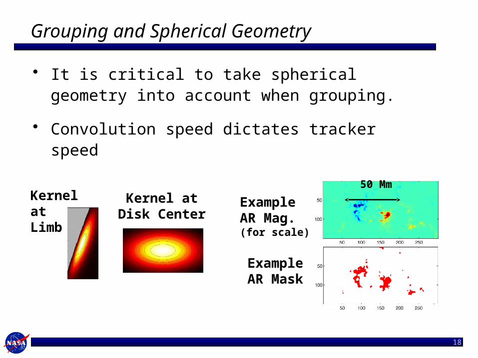
Grouping and Spherical Geometry

• It is critical to take spherical geometry into account when grouping.

• Convolution speed dictates tracker speed

18

Kernel atDisk Center

Kernelat Limb

50 Mm

ExampleAR Mag.(for scale)

ExampleAR Mask

19

Active Region Tracking: Grouping Example

MDI Labeling

2002 Sep. 02, 11:11 UTC

Convolved with Template

Identified Groups

20

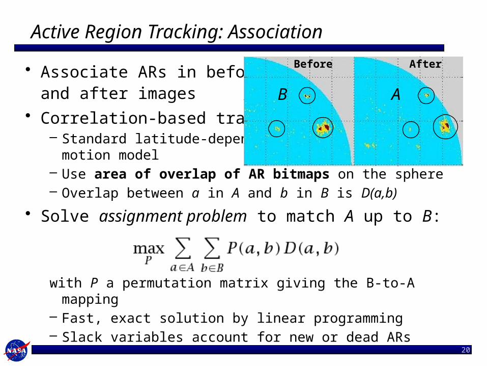
Active Region Tracking: Association

• Associate ARs in beforeand after images

• Correlation-based tracker– Standard latitude-dependent

motion model– Use area of overlap of AR bitmaps on the sphere– Overlap between a in A and b in B is D(a,b)

• Solve assignment problem to match A up to B:

with P a permutation matrix giving the B-to-A mapping– Fast, exact solution by linear programming– Slack variables account for new or dead ARs

AB

Before After

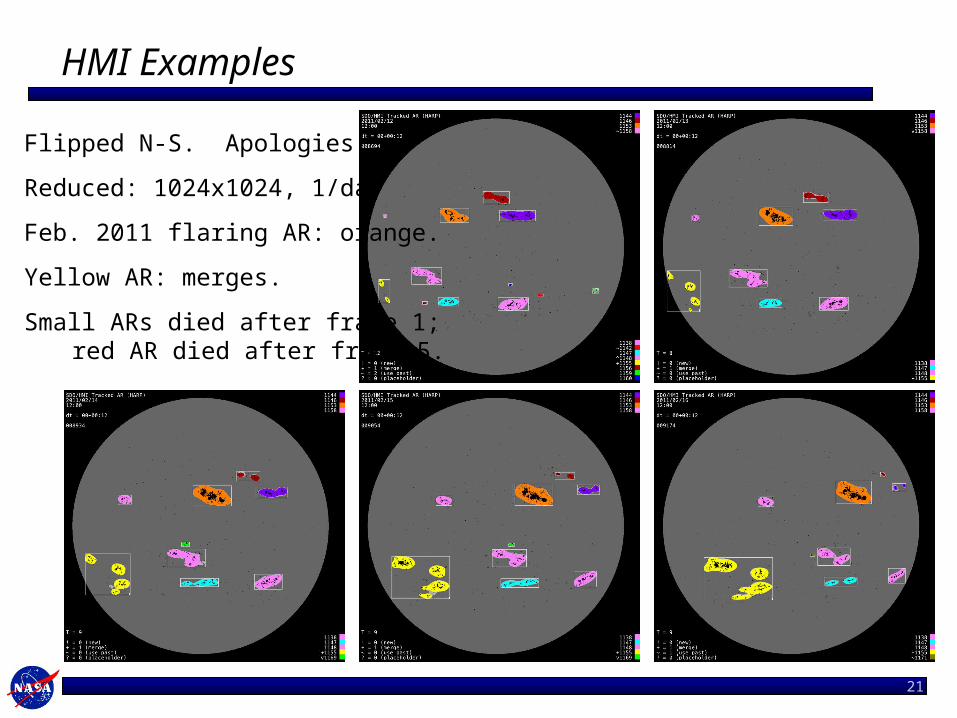
HMI Examples

21

Flipped N-S. Apologies!

Reduced: 1024x1024, 1/day

Feb. 2011 flaring AR: orange.

Yellow AR: merges.

Small ARs died after frame 1;red AR died after frame 5.

22

23

References

M. Turmon, H. Jones, J. Pap, O. Malanushenko, “Statistical feature recognition for multidimensional solar imagery”, Solar Physics, 04/2010.

The mixture modeling work appeared in:

Mixtures-2001, “Recent Developments in Mixture Modelling,” HamburgCompstat-2004, Prague, as “Symmetric Normal Mixtures”

Earlier work:

J. Pap, H. Jones, M. Turmon & L. Floyd, “Study of the SOHO/VIRGO Irradiance Variations using MDI and Kitt Peak images,” Proc. SOHO-11 Workshop, Davos, 2002.

H.P. Jones, M. Turmon, et al. “A comparison of feature classification methods for modeling solar irradiance variation,” 34th COSPAR Scientific Assembly, 2002.

The research described here was carried out in part by the Jet Propulsion Laboratory, California Institute of Technology, under contract with the National Aeronautics and Space Administration. Copyright 2011. All rights reserved. Government sponsorship acknowledged.