Algebraic proof theory for substructural logics:

cut-elimination and completions

Agata Ciabattonia, Nikolaos Galatosb, Kazushige Terui∗,c

aDepartment of Formal Languages, Vienna University of Technology, Favoritenstrasse 9-11,

1040 Wien, AustriabDepartment of Mathematics, University of Denver, 2360 S. Gaylord St., Denver, CO

80208, USAcResearch Institute for Mathematical Sciences, Kyoto University, Kitashirakawa Oiwakecho,

Sakyo-ku, Kyoto 606-8502, Japan

Abstract

We carry out a unified investigation of two prominent topics in proof theory andorder algebra: cut-elimination and completion, in the setting of substructurallogics and residuated lattices.

We introduce the substructural hierarchy – a new classification of logicalaxioms (algebraic equations) over full Lambek calculus FL, and show that astronger form of cut-elimination for extensions of FL and the MacNeille com-pletion for subvarieties of pointed residuated lattices coincide up to the level N2

in the hierarchy. Negative results, which indicate limitations of cut-eliminationand the MacNeille completion, as well as of the expressive power of structuralsequent calculus rules, are also provided.

Our arguments interweave proof theory and algebra, leading to an integrateddiscipline which we call algebraic proof theory.

Key words: Substructural logic, Gentzen system, residuated lattices,cut-elimination, structural rule, MacNeille completions2000 MSC: 03B47, 06F05, 03G10, 08B15

1. Introduction

The algebraic and proof-theoretic approaches to logic have traditionally de-veloped in parallel, non-intersecting ways. This paper is part of a project toidentify the connections between these two areas and apply methods and tech-niques from each field to the other in the setting of substructural logics. Theemerging discipline may be named algebraic proof theory. The main contri-bution of the paper is to reveal the connection between (a stronger form of)

∗Corresponding author. Partly supported by JSPS KAKENHI 21700041.Email addresses: agata@logic.at (Agata Ciabattoni), ngalatos@du.edu (Nikolaos

Galatos), terui@kurims.kyoto-u.ac.jp (Kazushige Terui)

Preprint submitted to Elsevier September 1, 2011

cut-elimination for sequent calculi and the MacNeille completion for the cor-responding algebraic models, established by interweaving proof theoretic andalgebraic arguments.

Sequent calculi have played a central role in proof theory (see, e.g., [43], [9],[35]). Strongly analytic sequent calculi – that is calculi in which proofs fromatomic assumptions only consist of formulas already contained in the statementto be proved – are useful for establishing various properties. These include con-sistency, conservativity and interpolation. Analyticity, as well as its strength-ened version referring to derivations from atomic assumptions, mainly followfrom the fundamental theorem of cut-elimination which states the redundancyof the cut rule. Sequent calculi have been proposed for various logics. Here weare interested in substructural logics (see, e.g., [20, 37]), i.e., logics which mayinvalidate some of the structural rules. They encompass among many othersclassical, intuitionistic, intermediate, fuzzy, linear and relevant logics. In gen-eral, a substructural logic is any axiomatic extension of full Lambek calculusFL, a calculus equivalent to Gentzen’s sequent calculus LJ for intuitionisticlogic without structural rules. In this setting, additional properties are oftenimposed on FL by means of axioms or structural rules. As cut-elimination isnot preserved in general under the addition of axioms, the following question isof great importance:

Given an axiom, is it possible to transform it into a “good” structuralrule— i.e. one which preserves strong analyticity when added to FL?

Substructural logics correspond to subvarieties of (pointed) residuated lat-tices (see, e.g., [26]), via a Tarski-Lindenbaum construction. The strong cor-respondence between them (known as algebraization), together with rich toolsfrom universal algebra, has allowed for a fruitful algebraic study of substructurallogics (see [20]). An important technique here is completion, that is to embeda given ordered algebraic structure into a complete one. Here we are interestedin a particular completion method known as the (Dedekind-)MacNeille comple-tion, which generalizes Dedekind’s embedding of the rational numbers into thereals [29]. It admits a nice abstract characterization due to [5, 38]. Moreover, itpreserves all existing joins and meets, hence is useful for proving completenessof predicate logics with respect to complete algebras, see [34]. Although theMacNeille completion applies to all individual residuated lattices, it may pro-duce a residuated lattice that is not in a given variety, containing the originalone. Hence an important question here is:

Given a variety of pointed residuated lattices, is it closed under Mac-Neille completions? Or equivalently, given an equation over residu-ated lattices, is it preserved by MacNeille completions?

The two questions, above raised in different contexts, are in fact deeplyrelated. The connection can be naively understood by noticing that both areconcerned with some conservativity properties (cf. Lemmas 5.13 and 5.19). How-ever, to establish the exact correspondence between strong analyticity and the

2

MacNeille completion and to demonstrate their limitations, it seems that it isnot enough to merely combine results of algebra and proof theory; it is necessaryto integrate techniques from each discipline in a more intimate and systematicway.

The emerging theory, called algebraic proof theory, consists of two basicideas:

1. Proof theoretic treatment of algebraic equations,

2. Algebraization of proof theoretic methods.

1. Proof theoretic treatment of algebraic equations. An important idea stemmingfrom proof theory is to classify logical formulas into a hierarchy according totheir syntactic complexity, i.e., how difficult they are to deal with. The mostprominent example is the arithmetical hierarchy in Peano arithmetic. Inspiredby the latter and the notion of polarity coming from proof theory of linearlogic [1], we introduce a hierarchy (Nn,Pn) on equations, called substructuralhierarchy (Section 3.1).

Another prominent feature of our proof-theoretic approach is a special em-phasis on quasiequations. Most of the algebraic contributions to our field havefocused on equational classes. However, even when the class of algebraic modelsis defined by equations, a reformulation of the latter into equivalent quasiequa-tions can be useful. This becomes apparent in view of the connection to prooftheory, where a transformation of axioms (equations) into suitable structuralrules (quasiequations) is essential for cut-elimination. Remarkably, such a trans-formation is also a key step when proving preservation under MacNeille com-pletions.

We describe a procedure, which applies to axioms/equations at a low levelin the substructural hierarchy (up to the class N2) and transforms them intoequivalent structural rules/quasiequations (Section 3). We also present a pro-cedure for transforming the generated rules/quasiequations into ‘analytic’ oneswhich behave well with respect to both strong analyticity and the MacNeillecompletion (Section 4). The latter procedure applies to any ‘acyclic’ structuralrule/quasiequation, or to any structural rule/quasiequation in presence of theweakening rule (integrality). These two procedures together allow the introduc-tion of strongly analytic sequent calculi for all logics semantically characterizedby (acyclic) N2-equations over residuated lattices. These calculi are uniformand their introduction is algorithmic.

2. Algebraization of proof theoretic methods. Syntactic proofs of cut-eliminationare often cumbersome and not modular in the sense that each time a new ruleis added to a sequent calculus cut-elimination has to be reproved from theoutset. More importantly, syntactic proofs are available only for predicativesystems, and not for second order logics with the full comprehension axiom.These situations have motivated the investigation of semantic proofs for cut-elimination (e.g., [39, 32, 33, 31, 6, 22, 19]) even though one loses concretealgorithms to eliminate cuts from a given proof, and so the claim should bemore precisely called cut admissibility.

3

As observed in [6], the algebraic essence of cut-elimination lies in the con-struction of a quasihomomorphism from an intransitive structure W (calledGentzen structure) to a complete (and transitive) algebra W+:

Wquasihom.

−→ W+.

The intransitive structure corresponds to a cut-free system, as the cut rule corre-sponds to transitivity of the algebraic inequation ≤. If the original structure W

is already transitive, the construction above is nothing but the MacNeille com-pletion. Thus cut-elimination and completion are of the same nature, and thecommon essence is well captured in terms of residuated frames, which abstractboth residuated lattices and sequent calculi for substructural logics [19].

We contribute to the algebraization of proof theory by showing that analyticstructural rules/quasiequations are preserved by the above construction. Similararguments have already appeared in [12, 11], but here the use of residuatedframes allows us to give a unified proof of the two facts that (i) analytic rulespreserve a strong form of cut-elimination (strong analyticity) and (ii) analyticquasiequations are preserved by MacNeille completions (Section 5).

Both strong analyticity and closure under completions imply some conser-vativity properties with respect to extensions with infinitary formulas. A prooftheoretic argument shows that conservativity in turn implies that the involvedstructural rules/quasiequations are equivalent to analytic ones (Section 6). Thisleads to the equivalence of statements (1)-(3) below for any set R of N2-equations/axioms or structural rules/quasiequations:

1. R is equivalent to a set of analytic structural rules which preserve stronganalyticity when added to (any infinitary extension of) FL.

2. The class of FL-algebras satisfying R is closed under MacNeille comple-tions.

3. Every infinitary extension of FL+R is a conservative extension of FL+R.

An example of an equation/axiom in N2 which does not satisfy any of (1)-(3) is also presented. This indicates the limitations of strong analyticity andMacNeille completions within N2. Our results also shed light on the expressivepower of structural sequent rules, which is discussed in Section7.

Related work. Syntactic and semantic conditions for a sequent calculus to admit(a stronger form of) cut elimination are contained, e.g., in [41, 14, 4, 3]. Whilethese works focus on calculi, our current project focuses on logics (defined byaxioms), and investigates under which conditions they admit a strongly analyticsequent calculus.

Also, the substructural hierarchy and the transformations of axioms intostructural rules were introduced in [12] for the commutative case and in [13]for the commutative and involutive case. While these two papers are prooftheoretic, [11] makes use of their ideas for purely algebraic purposes. The currentpaper unifies both directions.

4

Preservation of equations under completions is an old and mature topic,see e.g. the survey [24]. Among many works, paper [42] investigates MacNeillecompletions of arbitrary lattice expansions (which include FL-algebras). Themethodology in [42] provides a topological perspective on equations preservedby MacNeille completions, that is complementary to our proof theoretic per-spective.

Closely related to MacNeille completions are canonical extensions [27, 28](recall a deep result in [17]: preservation under MacNeille completions impliespreservation under canonical extensions for arbitrary monotone bounded latticeexpansions, which include bounded FL-algebras). Canonical extensions of FL-algebras are studied in [40]. Following some previous works, the paper identifiesa class of equations preserved by canonical extensions by means of a tree labelingalgorithm, that is complementary to our method. Finally, following [15], [16]contains a (quasi)equation-transformation procedure which is based on the so-called Ackermann’s lemma, as in the case of our transformation procedure (cf.Lemma 3.4).

2. Preliminaries

2.1. Full Lambek calculus and substructural logics

We start by recalling our base calculus: the sequent system FL. The for-mulas of FL are built from propositional variables p, q, r, . . . and constants 1(unit) and 0 by using binary logical connectives · (fusion), \ (right implica-tion), / (left implication), ∧ (conjunction) and ∨ (disjunction). FL sequentsare expressions of the form Γ ⇒ Π, where the left-hand-side (LHS) Γ is a finite(possibly empty) sequence of formulas of FL and the right-hand-side (RHS)Π is single-conclusion, i.e., it is either a formula or the empty sequence. Thesequent calculus rules of FL are displayed in Figure 1. Letters α, β stand forformulas, Π stands for either a formula or the empty set, and Γ,∆, . . . stand forfinite (possibly empty) sequences of formulas. ¬α and α ↔ β will be used asabbreviations for α\0 and (α\β)∧ (β\α) respectively, while αn and α(n) for theformula α · . . . · α and the sequence α, . . . , α (n times), respectively.

Roughly speaking, FL is obtained by dropping all the structural rules (ex-change (e), contraction (c), left weakening (i) and right weakening (o); seeFigure 2), from the sequent calculus LJ for intuitionistic logic. Also, FL (to-gether with ⊤ and ⊥ below) is the same as noncommutative intuitionistic linearlogic without exponentials.

Remark 2.1. Often, the constants ⊤ (true) and ⊥ (false) and the rules

Γ ⇒ ⊤⊤r

Γ1,⊥,Γ2 ⇒ Π⊥l

are added to the language and rules of FL, respectively; the resulting sequentcalculus is denoted by FL⊥. The results in our paper hold for both FL andFL⊥.

5

The notion of proof in FL (and in the mentioned extensions) is definedas usual. If there is a proof in FL of a sequent s from a set of sequents S,we write S ⊢seq

FLs. If Φ ∪ {ψ} is a set of formulas, we write Φ ⊢FL ψ, if

{ ⇒ φ : φ ∈ Φ} ⊢seqFL

⇒ ψ. Clearly, ⊢seqFL

and ⊢FL are consequence relations onthe sets of sequents and formulas, respectively. When no confusion arises, wewill omit the superscript and write simply ⊢FL for ⊢seq

FL.

The calculus FL serves as the main system for defining substructural logics,the latter being simply (the sentential part of) axiomatic extensions of FL. Asubstructural logic is simply a set of formulas closed under ⊢FL and substitution.

2.2. Polarities

Following [1], the logical connectives of FL⊥ are classified into two groups:connectives 1,⊥, ·,∨ (resp. 0,⊤, \, /,∧), for which the left (resp. right) logicalrule is invertible, are said to have positive (resp. negative) polarity. Here a ruleis invertible if the conclusion implies the premises. E.g., for (∨l) (cf. Figure 1)we have:

Γ1, α ∨ β,Γ2 ⇒ Π ⊣⊢FL⊥{Γ1, α,Γ2 ⇒ Π, Γ1, β,Γ2 ⇒ Π}

Connectives of the same polarity interact well with each other. Indeed, forpositive connectives,

α · 1 ↔ α, α ∨ ⊥ ↔ α, α · ⊥ ↔ ⊥, α · (β ∨ γ) ↔ (α · β) ∨ (α · γ)

are provable in FL⊥, while for negative connectives, we have:

α ∧ ⊤ ↔ α, (1 → α) ↔ α, (α→ ⊤) ↔ ⊤, (⊥ → α) ↔ ⊤,(α→ (β ∧ γ)) ↔ (α→ β) ∧ (α→ γ), ((α ∨ β) → γ) ↔ (α→ γ) ∧ (β → γ),

where α→ β stands for either α\β and β/α, uniformly in each formula.We stipulate that polarity is reversed on the left hand side of implications.

For instance, the ∨ on the left-hand side of → in the last equivalence is consid-ered negative.

Since connectives ∨,∧, · have units ⊥,⊤, 1 respectively, we will adopt a nat-ural convention: β1 ∨ · · · ∨ βm (resp. β1 ∧ · · · ∧ βm and β1 · · ·βm) stands for ⊥(resp. ⊤ and 1) if m = 0.

2.3. Structural rules

Structural rules are described by using three types of metavariables:

• metavariables for formulas: α, β, γ, . . .

• metavariables for sequences of formulas: Γ,∆,Σ, . . .

• metavariables for stoups (i.e., for either the empty set or a formula): Π.

6

Γ ⇒ α ∆1, α,∆2 ⇒ Π

∆1,Γ,∆2 ⇒ Π(cut)

α⇒ α (init) ⇒ 1(1r)

Γ1, α, β,Γ2 ⇒ Π

Γ1, α · β,Γ2 ⇒ Π(·l)

Γ ⇒ α ∆ ⇒ β

Γ,∆ ⇒ α · β(·r)

Γ1,Γ2 ⇒ Π

Γ1, 1,Γ2 ⇒ Π(1l)

Γ ⇒ α ∆1, β,∆2 ⇒ Π

∆1,Γ, α\β,∆2 ⇒ Π(\l)

α,Γ ⇒ β

Γ ⇒ α\β(\r) Γ ⇒

Γ ⇒ 0(0l)

Γ ⇒ α ∆1, β,∆2 ⇒ Π

∆1, β/α,Γ,∆2 ⇒ Π(/l)

Γ, α⇒ β

Γ ⇒ β/α(/r)

0 ⇒(0r)

Γ1, α,Γ2 ⇒ Π Γ1, β,Γ2 ⇒ Π

Γ1, α ∨ β,Γ2 ⇒ Π(∨l) Γ ⇒ α

Γ ⇒ α ∨ β(∨r1)

Γ ⇒ β

Γ ⇒ α ∨ β(∨r2)

Γ1, α,Γ2 ⇒ Π

Γ1, α ∧ β,Γ2 ⇒ Π(∧l1)

Γ1, β,Γ2 ⇒ Π

Γ1, α ∧ β,Γ2 ⇒ Π(∧l2)

Γ ⇒ α Γ ⇒ β

Γ ⇒ α ∧ β(∧r)

Figure 1: Inference Rules of FL

Some examples of structural rules are displayed in Figure 2. An instance ofthe contraction rule (c) is for example

p ∧ q, 0, r ∨ 1, r ∨ 1, p/q ⇒

p ∧ q, 0, r ∨ 1, p/q ⇒

which is obtained by instantiating Γ by the sequence p∧q, 0 of concrete formulas,α by the concrete formula r ∨ 1, ∆ by p/q, and Π by the empty set. Therefore,(c) represents (or specializes to) many rules, so formally it should be called ametarule. In practice, the distinction between metarules and rules is understoodimplicitly and both are refereed to as rules.

Note that the following is not an instance of (c)

p ∧ q, 0, r ∨ 1, s, r ∨ 1, s, p/q ⇒

p ∧ q, 0, r ∨ 1, s, p/q ⇒

but is an instance of (seq-c) with instantiation of Σ by the concrete sequencer ∨ 1, s. Hence (c) and (seq-c) are different rules, even though they have thesame strength. Similar distinctions may be observed on the right hand side ofa sequent. It is instructive to think about the differences among

Γ ⇒ β

α,Γ ⇒ β(w1) Γ ⇒

α,Γ ⇒(w2) Γ ⇒ Π

α,Γ ⇒ Π(w3)

7

Γ,∆ ⇒ Π

Γ, α,∆ ⇒ Π(i) Σ ⇒

Σ ⇒ α(o)

Γ, α, α,∆ ⇒ Π

Γ, α,∆ ⇒ Π(c)

Γ, α, β,∆ ⇒ Π

Γ, β, α,∆ ⇒ Π(e)

Γ, α,∆ ⇒ Π

Γ, α, α,∆ ⇒ Π(exp)

m︷ ︸︸ ︷α, . . . , α⇒ β

α, . . . , α︸ ︷︷ ︸

n

⇒ β(knotnm)

Γ,Σ,Σ,∆ ⇒ Π

Γ,Σ,∆ ⇒ Π(seq-c)

Σ,Σ ⇒

Σ ⇒(wc)

Γ,Σ1,∆ ⇒ Π Γ,Σ2,∆ ⇒ Π

Γ,Σ1,Σ2,∆ ⇒ Π(min)

Σ ⇒ Γ,∆ ⇒ Π

Γ,Σ,∆ ⇒ Π(mix)

{Γ,Σi1 , . . . ,Σim,∆ ⇒ Π}i1,...,im∈{1,...,n}

Γ,Σ1, . . . ,Σn,∆ ⇒ Π(anl-knotnm)

Figure 2: Examples of Structural Rules

The rule (w1) may be applied only when there is a formula on the RHS, while(w2) only when the RHS is empty; (w3) can be applied in both cases.

In general, a single-conclusion structural rule (structural rule for short) isany rule of the form (n ≥ 0)

Υ1 ⇒ Ψ1 · · · Υn ⇒ Ψn

Υ0 ⇒ Ψ0(r)

where each Υi is a specific sequence of metavariables (allowed to be of bothtypes: metavariables for formulas or for sequences of formulas), and each Ψi iseither empty, a metavariable for formulas (α), or a metavariable for stoups (Π).Υi ⇒ Ψi, with i = 0, . . . , n are called metasequents.

Given a set R of structural rules, we denote by FLR the system obtained byadding to FL the rules in R, and by ⊢seq

FLRthe associated consequence relation

(often simply written ⊢FLR).

Two rules (r0) and (r1) are equivalent (in FL) if the relations ⊢FL(r0)and

⊢FL(r1)coincide. This holds when the conclusion of (r0) (and resp. of (r1)) is

derivable from its premises in FL(r1) (resp. FL(r0)). The definition naturallyextends to sets of rules.

2.4. Algebraic semantics

The system FL is algebraizable and its algebraic semantics is the class ofpointed residuated lattices, also known as FL-algebras.

A residuated lattice is an algebra A = (A,∧,∨, ·, \, /, 1), such that (A,∧,∨)is a lattice, (A, ·, 1) is a monoid and for all a, b, c ∈ A,

a · b ≤ c iff b ≤ a\c iff a ≤ c/b.

8

We refer to the last property as residuation.An FL-algebra is an expansion of a residuated lattice with an additional

constant element 0, namely an algebra A = (A,∧,∨, ·, \, /, 1, 0), such that(A,∧,∨, ·, \, /, 1) is a residuated lattice. In residuated lattices and FL-algebras,we will write a ≤ b instead of a = a ∧ b (or equivalently, a ∨ b = b). Note thata = b is equivalent to 1 ≤ a\b ∧ b\a.

The classes RL and FL of residuated lattices and FL-algebras, respectively,can be defined by equations. Consequently, they are varieties, namely classes ofalgebras closed under subalgebras, homomorphic images and direct products.

Given a class K of FL-algebras, we say that the equation s = t is a semanticalconsequence of a set of equations E relative to K, in symbols

E |=K s = t,

if for every algebra A ∈ K and every valuation f into A, if f(u) = f(v), for all(u = v) ∈ E, then f(s) = f(t). Clearly, |=K is a consequence relation on the setof equations.

All three relations ⊢seqFL

, ⊢FL and |=FL are equivalent ; see [21] and [20]. This isalso known as the algebraization of FL. Identifying terms of residuated latticesand propositional formulas of FL, we can give translations between sequents,formulas and equations as follows. Given a sequent α1, . . . , αn ⇒ α, the corre-sponding equation and formula are α1 · . . . · αn ≤ α and (α1 · . . . · αn)\α; forα1, . . . , αn ⇒ we have α1 · . . . ·αn ≤ 0 and (α1 · . . . ·αn)\0. To a formula α, weassociate ⇒ α and 1 ≤ α.

In view of the algebraization, we have that for a set of sequents S ∪ {s},

S ⊢seqFL

s iff ε[S] |=FL ε(s)

where ε(s) is the equation corresponding to s.Bounded FL-algebras are expansions of FL-algebras that happen to be bounded

as lattices with two new constants interpreting the bounds (⊥, ⊤). The corre-sponding class FL⊥ of algebras is the equivalent algebraic semantics of FL⊥. Theexistence of bounds excludes interesting algebras, like lattice-ordered groups.

2.5. Interpretation of structural rules

To avoid confusion between the connectives of our language and the con-nectives of classical logic, we denote the latter by and and =⇒. Recall that aquasiequation is a strict universal Horn first-order formula of the form

ε1 and . . . and εn =⇒ ε0, (q)

where ε0, . . . , εn are equations. ε1, . . . , εn are the premises and ε0 is the conclu-sion. An FL-algebra A satisfies (q) if {ε1, . . . , εn} |={A} ε0. Two quasiequations(q1) and (q2) are equivalent if they are satisfied by the same class of FL-algebras.

We now introduce a class of quasiequations corresponding to structural rules.

Definition 2.2. A quasiequation ε1 and . . . and εn =⇒ ε0 is structural if eachεi (0 ≤ i ≤ n) is an inequation t ≤ u where t is a (possibly empty) product ofvariables and u is either a variable or 0.

9

Every structural rule can be interpreted by a structural quasiequation as fol-lows. Let Υ be a sequence of metavariables, and Ψ either empty, a metavariableα for formulas, or Π for stoups. Given a fixed bijection between the denumer-able sets of variables and metavariables, we define the interpretation Υ• of Υas the term in the language of FL obtained by replacing the metavariables bytheir corresponding variables and comma by the connective · (fusion); if Υ isempty, then Υ• = 1. For example, if Υ = α,Γ, β,Γ, then Υ• = xyzy. Theinterpretation (Υ ⇒ Ψ)• of a metasequent Υ ⇒ Ψ is defined to be Υ• ≤ 0 if Ψis empty, Υ• ≤ α•, if Ψ = α, and Υ• ≤ Π•, if Ψ = Π.

The interpretation of a structural rule (let s, s1, . . . , sn be metasequents)

s1 · · · sn

s (r)

is defined to be the structural quasiequation

s•1 and . . . and s•n =⇒ s•. (r•)

For a set R of structural rules, we define R• = {(r•) : (r) ∈ R}.Notice that the interpretation disregards the distinction between metavari-

ables for formulas and those for sequences of formulas. Hence there is somefreedom when reading back a structural rule from a given structural quasiequa-tion.

Given a set Q of quasiequations, FLQ will denote the class of all FL-algebrasthat satisfy Q; clearly FLQ is a quasi-variety. It follows from the algebraizationand from general considerations on the equivalence of consequence relations (seeProposition 7.4 of [36]) that the relations ⊢seq

FLRand |=FLR• are equivalent. In

particular, for a set S ∪ {s} of sequents and a set R of structural rules,

S ⊢seqFLR

s iff ε[S] |=FLR• ε(s)

where ε(s) is the equation corresponding to s.

3. Equations and structural rules

A substructural logic is by definition an extension of FL with axioms. How-ever, if one simply adds an axiom to FL, one easily loses cut-elimination, theraison d’etre of proof theory. Hence to apply proof theoretic techniques tosubstructural logics, one needs to structuralize axioms, namely to transformthem into suitable structural rules. In algebraic terms, this corresponds to thetransformation of equations into structural quasiequations. It is a crucial stepwhen proving that some equations are preserved by MacNeille completions (Def.5.14).

In this section we investigate which axioms can be structuralized, or equiv-alently, which equations can be transformed into structural quasiequations.

10

Class Equation Name Structural ruleN1 xx ≤ x expansion (exp)N2 xy ≤ yx exchange (e)

x ≤ 1 left weakening (i)0 ≤ x right weakening (o)x ≤ xx contraction (c)xn ≤ xm knotted (n,m ≥ 0) (knotnm)x ∧ ¬x ≤ 0 weak contraction (wc)

P2 1 ≤ x ∨ ¬x excluded middle none (Prop. 7.1)1 ≤ (x\y) ∨ (y\x) prelinearity none (Prop. 7.1)

N3 x(x\y) = x ∧ y = (y/x)x divisibility none (Prop. 7.1)x ∧ (y ∨ z) ≤ (x ∧ y) ∨ (x ∧ z) distributivity none (Cor. 7.4)

P3 1 ≤ ¬x ∨ ¬¬x weak excluded middle none (Prop. 7.1)

Figure 3: Some Known Equations

3.1. Substructural hierarchy

To address the problem systematically, we introduce below a classification(Pn,Nn) of the terms of FL⊥ which is analogous to the arithmetical hierarchy(Σn,Πn). Our hierarchy, introduced in [12] for the commutative case, is basedon polarities; see Section 2.2.

Definition 3.1. For each n ≥ 0, the sets Pn,Nn of terms are defined as follows:

(0) P0 = N0 = the set of variables.

(P1) 1,⊥ and all terms of Nn belong to Pn+1.

(P2) If t, u ∈ Pn+1, then t ∨ u, t · u ∈ Pn+1.

(N1) 0,⊤ and all terms of Pn belong to Nn+1.

(N2) If t, u ∈ Nn+1, then t ∧ u ∈ Nn+1.

(N3) If t ∈ Pn+1 and u ∈ Nn+1, then t\u, u/t ∈ Nn+1.

Symbolically, we may then write

Pn+1 = 〈Nn〉∨ ,∏ and Nn+1 = 〈Pn ∪ {0}〉∧ ,Pn+1→,

namely Pn+1 is the set generated from Nn by means of finite (possibly empty)joins and products, and Nn+1 is generated by Pn ∪ {0} by means of finite(possibly empty) meets and divisions with denominators from Pn+1.

By residuation, any equation ε can be written as 1 ≤ t. We say that εbelongs to Pn (Nn, resp.) if t does.

Figure 3 classifies some known equations. In terms of logic, they correspondto axioms; for instance, weak contraction and prelinearity correspond to theaxioms ¬(α ∧ ¬α) and (α\β) ∨ (β\α), respectively (see Section 2.4).

11

P2 N2

P1 N1

P0 N0

p

p

p

p

p

p

p

p

p

6

p

p

p

p

p

p

p

p

p

6

6

��

��� 6

@@

@@I

6

��

��� 6

@@

@@I

Figure 4: The Substructural Hierarchy

Proposition 3.2.

1. Every term belongs to some Pn and Nn.

2. Pn ⊆ Pn+1 and Nn ⊆ Nn+1 for every n.

Hence the classes Pn, Nn constitute a hierarchy as depicted in Figure 4,which we call the substructural hierarchy.

Terms in each class admit the following normal forms.

Lemma 3.3.

(P) If t ∈ Pn+1, then t is equivalent to ⊥ or u1 ∨ · · · ∨ um, where each ui is aproduct of terms in Nn.

(N) If t ∈ Nn+1, then t is equivalent to ⊤ or∧

1≤i≤m li\ui/ri, where each ui

is either 0 or a term in Pn, and each li and ri are products of terms inNn.

Proof. We will prove the lemma by simultaneous induction of the two state-ments.

Statement (P) is clear for t = ⊥. The case t = 1 is a special case for m = 1and u1 the empty product. If (P) holds for t, u ∈ Pn+1, then it clearly holds fort ∨ u. For t · u, we use the fact that multiplication distributes over joins.

Statement (N) is clear for t = ⊤. For t = 0 we take m = 1, l1 = r1 = 1and u1 = 0. If (N) holds for t, u ∈ Nn+1, then it clearly holds for t ∧ u. Ift ∈ Pn+1 and u ∈ Nn+1, we know that t = t1 ∨ · · · ∨ tm, for ti a productof terms in Nn, where m = 0 yields the empty join t = ⊥. We have t\u =(t1∨· · ·∨ tm)\u = (t1\u)∧· · ·∧ (tm\u). Moreover, by the induction hypothesis,for all j ∈ {1, . . . ,m}, tj\u = tj\(

∧

1≤i≤k li\ui/ri) =∧

1≤i≤k tj\(li\ui/ri) =∧

1≤i≤k(litj)\ui/ri; the empty meet ⊤ is obtained for k = 0.

12

As a consequence of the above lemma, every equation ε in N2 is equivalentto a finite set NF (ε) of equations of the form t1 · · · tm ≤ u, where u = 0 oru1∨· · ·∨uk and each ui is a product of variables. Furthermore, each ti is of theform

∧

1≤j≤n lj\vj/rj , where vj = 0 or a variable, and lj and rj are products ofvariables. We call NF (ε) the normal form of ε.

In the sequel, we frequently use the following lemma, corresponding to Ack-ermann’s Lemma in [15, 16].

Lemma 3.4. A quasiequation (q) ε1 and . . . and εn =⇒ t1 · · · tm ≤ u is equiv-alent to either one of

ε1 and . . . and εn and u ≤ x0 =⇒ t1 · · · tm ≤ x0 (q′)

ε1 and . . . and εn and x1 ≤ t1 and . . . and xm ≤ tm =⇒ x1 · · ·xm ≤ u (q′′)

where x0, . . . , xm are fresh variables.

Proof. We will prove the equivalence of (q) and (q′). Assume the premises of(q′). Then (q) entails t1 · · · tm ≤ u. Since u ≤ x0 by assumption, we havet1 · · · tm ≤ x0. For the converse direction, note that (q′) with x0 instantiatedby u entails (q).

3.2. From N2-equations to structural quasiequations

We show that the equations in N2 correspond to structural quasiequations,and hence to structural rules. Our proof is constructive and provides a methodto generate those quasiequations (see also the corresponding result in [12] forHilbert axioms over FL⊥ with exchange).

Theorem 3.5. Every equation in N2 is equivalent to a finite set of structuralquasiequations.

Proof. Let ε be an equation in N2 and let t1 · · · tm ≤ u ∈ NF (ε). By Lemma3.4, ε is equivalent to a quasiequation

x1 ≤ t1 and · · · and xm ≤ tm =⇒ x1 · · ·xm ≤ u,

where x1, . . . , xm are fresh variables. Since each ti is of the form∧

1≤j≤n lj\vj/rj ,xi ≤ ti can be replaced with n premises l1xir1 ≤ v1, . . . , lnxirn ≤ vn. We applythis replacement to all xi ≤ ti. If u is 0, then the resulting quasiequation isalready structural. Otherwise, u = u1 ∨ · · · ∨ uk. We replace the conclusion byx1 · · ·xm ≤ x0 and add k premises u1 ≤ x0, . . . , uk ≤ x0 with x0 a fresh vari-able. The resulting quasiequation is structural, and is equivalent to the originalone by Lemma 3.4.

Example 3.6. Using the algorithm contained in the proof of the theorem above,the weak contraction axiom ¬(α ∧ ¬α) is turned into an equivalent structural

13

rule. Indeed, it corresponds to the equation x ∧ ¬x ≤ 0 and is successivelytransformed as follows:

−→ z ≤ x ∧ ¬x =⇒ z ≤ 0,−→ z ≤ x and z ≤ ¬x =⇒ z ≤ 0,−→ z ≤ x and xz ≤ 0 =⇒ z ≤ 0.

From the last quasiequation, one can read back a structural rule

β ⇒ α α, β ⇒

β ⇒(wc′)

.

To obtain the final form (wc) which preserves strong analyticity (see Figure2), we will apply the transformation in Section 4.2 (analytic completion); seeExample 4.10.

3.3. From structural quasiequations to N2-equations?

Having established that N2-equations correspond to structural quasiequa-tions, we may ask the converse question. Namely, do all structural quasiequa-tions correspond to N2-equations? If not, do they correspond to equations atall? The following proposition provides a negative answer to both questions. Wealso identify a large class of structural quasiequations (N2-solvable quasiequa-tions) which correspond to N2-equations.

Proposition 3.7. Not every structural quasiequation is equivalent to an equa-tion.

Proof. Consider the quasiequation 1 ≤ 0 ⇒ x2 ≤ 0. We construct an FL-algebraA = (A,∧,∨, ·, \, /, 1, 0) which satisfies the quasiequation and a homomorphicimage of A which does not. Hence the quasiequation cannot be equivalent toan equation.

As A we take the set {⊥, a, 1,⊤}, where 0 = a and ⊥ < a < 1 < ⊤. Now, A

is completely specified by defining multiplication. We define ⊥ as an absorbingelement for A (⊥x = x⊥ = ⊥), ⊤ as an absorbing element for {a, 1,⊤} and a asan absorbing element for {a, 1}. It is easy to see that A is a residuated lattice(which is denoted by T3[2] in [18]) that satisfies the quasiequation vacuously.

We redefine 0 = 1 in the subalgebra of A on the set {⊥, 1,⊤} to obtain B.It is easy to see that the map that sends a to 1 and fixes the other elements isa homomorphism from A to B, but B does not satisfy the quasiequation.

Remark 3.8. The argument above can be repeated for many structural quasiequa-tions with single premise 1 ≤ 0 and a non-valid equation as conclusion.

We now give a sufficient condition for a structural quasiequation to be equiv-alent to an equation.

Definition 3.9. A structural quasiequation

t1 ≤ u1 and . . . and tn ≤ un =⇒ t ≤ u,

is said to be solvable if there is a substitution σ, called a solution, such that thefollowing holds in all FL-algebras:

14

(solv1) σ(ti) ≤ σ(ui) for all 1 ≤ i ≤ n, and

(solv2) ti ≤ ui for all 1 ≤ i ≤ n implies x ≤ σ(x) for every x occurring in t, andσ(x) ≤ x for x occurring in u (and σ(x) = x for x occurring in both).

It is called N2-solvable if σ(t) ≤ σ(u) is an N2-equation.

The structural quasiequation constructed in the proof of Theorem 3.5 is N2-solvable; indeed, the substitution σ given by σ(xi) = ti for 1 ≤ i ≤ m andσ(x0) = u provides a solution.

Proposition 3.10. Every solvable (resp. N2-solvable) quasiequation is equiva-lent to an equation (resp. N2-equation).

Proof. We will show that a structural quasiequation

t1 ≤ u1 and . . . and tn ≤ un =⇒ t ≤ u (q)

with solution σ is equivalent to the equation

σ(t) ≤ σ(u). (e)

Assume that (e) holds. Given the premises of (q), we obtain x ≤ σ(x) when xoccurs in t and σ(x) ≤ x when u = x by condition (solv2). Therefore, (e) yieldst ≤ σ(t) ≤ σ(u) ≤ u, the conclusion of (q).

Conversely, if (q) holds, then every substitution instance holds, as well. Sowe have

σ(t1) ≤ σ(u1) and . . . and σ(tn) ≤ σ(un) =⇒ σ(t) ≤ σ(u). (σ(q))

By condition (solv1), all the premises of (σ(q)) hold, so we get σ(t) ≤ σ(u).

We present below two classes of N2-solvable quasiequations. Let us call astructural quasiequation

t1 ≤ u1 and . . . and tn ≤ un =⇒ t ≤ u (q)

pivotal if one can find a variable xi (a pivot) in each ti which does not belongto {u1, . . . , un}.

Proposition 3.11. Every pivotal quasiequation is N2-solvable.

Proof. If (q) is pivotal, it can be written as

l1x1r1 ≤ u1 and . . . and lnxnrn ≤ un =⇒ t ≤ u,

where x1, . . . , xn are not necessarily distinct, and may occur in some li, ri, butnot in any ui. Define a substitution σ by

σ(xi) = xi ∧∧

lj\uj/rj

15

for 1 ≤ i ≤ n, where the meet∧lj\uj/rj is built from those premises ljxjrj ≤ uj

such that xj = xi. Let σ(z) = z for other variables z. We then have σ(y) ≤ yfor every variable y and σ(uk) = uk for every 1 ≤ k ≤ n.

Now σ satisfies condition (solv1), since

σ(lk)σ(xk)σ(rk) ≤ lk(lk\uk/rk)rk ≤ uk = σ(uk).

As to (solv2), the premises of (q) imply xi ≤∧lj\uj/rj for 1 ≤ i ≤ n. Hence

xi = σ(xi).Finally, σ(t) ≤ σ(u) clearly belongs to N2 since it is obtained by substituting

N1-terms into the N1-equation t ≤ u.

Example 3.12. The quasiequation xy ≤ x and x2y ≤ x =⇒ yx ≤ y is pivotalwith the choice of pivot y for both premises. It admits a solution σ(y) =y ∧ (x\x) ∧ (x2\x) and is equivalent to the N2-equation σ(y)x ≤ σ(y).

The notion of pivotality is motivated by the need of excluding premises withinevitable vicious cycles (cf. Definition 4.1) like

x y ≤ x and y x ≤ y =⇒ y ≤ x.

However, under certain conditions, some structural quasiequations are solvableeven with such cycles. We call a structural quasiequation one-variable if itspremises involve only one variable x and do not contain any of 1 ≤ x, x ≤ 0and 1 ≤ 0.

Proposition 3.13. Every one-variable quasiequation is N2-solvable.

Proof. Suppose that the quasiequation is of the form

xn1 ≤ u1 and . . . and xnk ≤ uk =⇒ t ≤ u

where each ui is either x or 0. By definition and since premises of the form x ≤ xare redundant, we may assume n1, . . . , nk ≥ 2. We claim that the substitution

σ(x) = x ∧ (u1/xn1−1) ∧ . . . ∧ (uk/x

nk−1)

gives rise to a solution.To check (solv1) we need to verify that σ(x)ni ≤ σ(ui) for 1 ≤ i ≤ k. If

ui = 0, we have

σ(x)ni ≤ (ui/xni−1)xni−1 ≤ ui = σ(ui).

On the other hand, if ui = x, we need to show that

σ(x)ni ≤ x ∧ (u1/xn1−1) ∧ . . . ∧ (uk/x

nk−1).

We will show that the left hand side is less than or equal to each of the termson the right hand side.

16

As before, we have σ(x)ni ≤ (ui/xni−1)xni−1 ≤ ui = x. Furthermore, for

every 1 ≤ r ≤ k we have

σ(x)nixnr−1 ≤ (ur/xnr−1)(x/xni−1)xni−2xnr−1 ≤ ur.

So σ(x)ni ≤ ur/xnr−1.

Finally, it is easy to see that condition (solv2) holds.

To sum up, we have obtained:

Corollary 3.14. Every N2-equation is equivalent to a set of N2-solvable quasiequa-tions. Conversely, every N2-solvable quasiequation (e.g., pivotal or one-variableones) is equivalent to an N2-equation.

In terms of logic, the first statement means that every N2-axiom can bestructuralized in the single-conclusion sequent calculus. The second statementcan also be rephrased accordingly.

In Section 7, we will show that “good” structural quasiequations (acyclicquasiequations that lack 1 ≤ 0 premises) are equivalent to N2-equations.

4. Analytic Completion

We have described a procedure for transforming N2-axioms/equations intostructural rules/quasiequations. However, this is not the end of the story, sincenot all structural rules preserve cut admissibility once added to FL. For in-stance, (cut) is not redundant in FL extended with the contraction rule (c)in Fig. 2, see e.g. [41]. We will see below that, among structural rules, acyclicones can always be transformed into equivalent analytic structural rules, whichpreserve strong analyticity once added to FL. The transformation is also im-portant for a purely algebraic purpose: to show preservation of quasiequationsunder MacNeille completions.

In Section 4.1, we describe a procedure (we refer to it as analytic completion)by means of which any acyclic quasiequation is transformed into an analytic one.The procedure also applies to any set of structural quasiequations (withoutthe assumption of acyclicity) in presence of integrality x ≤ 1 (left weakening).Our current procedure formalizes and extends to the non-commutative case theprocedure sketched in [12] (see also Section 6 of [41] for its origin). In Section4.2, we illustrate what analytic completion amounts to in terms of structuralrules.

4.1. Analytic completion of structural quasiequations

Let us begin with defining two classes of structural quasiequations.

Definition 4.1. Given a structural quasiequation (q) we build its dependencygraph D(q) in the following way:

• The vertices of D(q) are the variables occurring in the premises (we donot distinguish occurrences).

17

• There is a directed edge x −→ y in D(q) if and only if there is a premiseof the form lxr ≤ y.

(q) is said to be acyclic if the graph D(q) is acyclic (i.e., has no directed cyclesor loops).

The terminology naturally extends to structural rules as well. Also, supposethat an N2-equation ε is transformed into a set Q of structural quasiequationsby the procedure described in the proof of Theorem 3.5. We say that ε is acyclicif all quasiequations in Q are.

Example 4.2. A structural quasiequation that is not acyclic is xy ≤ x =⇒yx ≤ y, or the structural quasiequation xy ≤ z and z ≤ x =⇒ yxz ≤ y.

Definition 4.3. An analytic quasiequation is a structural quasiequation

t1 ≤ u1 and . . . and tn ≤ un =⇒ t0 ≤ u0

which satisfies the following conditions:

Linearity t0 is a (possibly empty) product of distinct variables x1, . . . , xm.

Separation u0 is either 0 or a variable x0 which is distinct from x1, . . . , xm.

Inclusion Each ti (1 ≤ i ≤ n) is a (possibly empty) product of some variablesfrom {x1, . . . , xm} (here repetition is allowed). Each ui (1 ≤ i ≤ n) iseither 0 or u0.

Given an acyclic quasiequation

ε1 and . . . and εn =⇒ ε0 (q0)

we transform it into an analytic one in two steps.

1. Restructuring. Suppose that ε0 is y1 · · · ym ≤ u. Let x0, x1, . . . , xm be freshvariables which are distinct from each other. Depending on whether u is 0 or avariable, we transform (q0) into either

ε1, . . . , εn and x1 ≤ y1, . . . , xm ≤ ym =⇒ x1 · · ·xm ≤ 0, (q1)

or

ε1, . . . , εn and x1 ≤ y1, . . . , xm ≤ ym and u ≤ x0 =⇒ x1 · · ·xm ≤ x0. (q2)

(q1) (or (q2)) is equivalent to (q0) by Lemma 3.4, is acyclic since x0, . . . , xm

are fresh, satisfies linearity, separation and

Exclusion none of x1, . . . , xm appears on the RHS of a premise, and x0 doesnot appear on the LHS of a premise.

18

2. Cutting. To obtain a quasiequation satisfying the inclusion condition, we haveto eliminate redundant variables from the premises, i.e., variables other thanx0, . . . , xm. We describe below how to remove such variables while preservingacyclicity and exclusion.

Let z be any redundant variable. If z appears only in the RHS of premises,we simply remove all such premises t1 ≤ z, . . . , tk ≤ z from the quasiequation.The resulting quasiequation is not weaker than the original one since it hasless premises. To show that it is not stronger either, observe that premisesti ≤ z in the original quasiequation hold with instantiation of z by

∨ti, and

the instantiation does not affect the other premises and conclusion. Hence theoriginal quasiequations implies the new one.

If z appears only in the LHS of premises, say l1zr1 ≤ u1, . . . , lkzrk ≤ uk, weargue similarly, this time instantiating z by

∧li\ui/ri.

Otherwise, z appears both in the RHS and LHS. Let SR = {si ≤ z : 1 ≤i ≤ k} and SL = {tj(z, . . . , z) ≤ uj : 1 ≤ j ≤ l} be sets of premises whichinvolve z on the RHS and LHS, respectively (where all occurrences of z in tjare displayed). By acyclicity, SR and SL are disjoint. We replace SR ∪SL with

SC = {tj(si1 , . . . , sin) ≤ uj : 1 ≤ j ≤ l and i1, . . . , in ∈ {1, . . . , k}}

The resulting quasiequation implies the original one, in view of transitivity.To show the converse, assume the premises of the new one. By instantiatingz =

∨si, all premises in SR hold and all premises in SL follow from SC , since

tj(∨si, . . . ,

∨si) =

∨tj(si1 , . . . , sin

) ≤ uj . Hence the original quasiequationyields the conclusion.

Note that acyclicity and exclusion are preserved and that the number ofredundant variables decreased by one. Repeating this process, we obtain aquasiequation satisfying exclusion which has no redundant variable. Such aquasiequation satisfies also the inclusion condition, and therefore it is analytic.

Remark 4.4. The assumption of acyclicity is redundant in presence of integral-ity x ≤ 1 (left weakening). Indeed, acyclicity was essentially used only in thelast step where we needed to ensure that SL and SR are disjoint. If an equationbelongs to both SL and SR, then it is of the form t(z, . . . , z) ≤ z, which can besafely removed as it follows directly from integrality.

We have thus proved:

Theorem 4.5. Every acyclic quasiequation is equivalent to an analytic one.The same holds for any structural quasiequation in presence of integrality x ≤ 1.

4.2. Analytic completion of structural rules

We apply the procedure in the previous section to acyclic structural rules(or any structural rules in presence of left weakening) in order to transformthem into analytic rules. The latter will be shown in Section 5.5 to preserve (astronger form of) cut admissibility once added to FL. These results, together

19

with the procedure contained in the proof of Theorem 3.5, allow for the au-tomated definition of strongly analytic sequent calculi for logics semanticallycharacterized by (acyclic) N2-equations over residuated lattices.

Any acyclic structural rule (r) can be interpreted as an acyclic quasiequation(r•) (see Section 2.5). By applying to the latter the completion procedure inthe previous section we obtain an analytic quasiequation.

In the sequel, we describe a precise way of reading back an analytic rule fromthe analytic quasiequation.

Definition 4.6. A structural rule (r) is analytic if it has one of the forms

Υ1 ⇒ . . . Υk ⇒ Γ,Υk+1,∆ ⇒ Π . . . Γ,Υn,∆ ⇒ Π

Γ,Υ0,∆ ⇒ Π(r1)

Υ1 ⇒ . . . Υn ⇒Υ0 ⇒

(r2)

and satisfies:

Linearity Υ0 is a sequence of distinct metavariables Σ1, . . . ,Σm for sequences.

Separation Γ and ∆ are distinct metavariables for sequences different fromΣ1, . . . ,Σm, and Π is a metavariable for stoups.

Inclusion Each Υi (1 ≤ i ≤ n) is a sequence of some metavariables from{Σ1, . . . ,Σm} (here repetition is allowed).

Example 4.7. With reference to Figure 2, the rules (seq-c), (wc), (min), (mix)and (anl-knotnm) are analytic, while the remaining ones are not.

We can associate to each analytic quasiequation

ε1 and . . . and εn =⇒ ε0 (q)

an analytic structural rule (q◦) as follows. Assume that ε0 is of the formx1 · · ·xm ≤ x0; the construction below subsumes the case of x1 . . . xm ≤ 0.We associate to each xi (1 ≤ i ≤ m) a metavariable Σi for sequences, and tox0 three metavariables Γ,∆ and Π. If εj is of the form xi1 · · ·xik

≤ 0 withi1, . . . , ik ∈ {1, . . . ,m}, let ε◦j be the sequent Σi1 , . . . ,Σik

⇒ , and if εj is ofthe form xi1 · · ·xik

≤ x0, let ε◦j be Γ,Σi1 , . . . ,Σik,∆ ⇒ Π. We thus obtain a

structural ruleε◦1 · · · ε◦n

ε◦0(q◦)

which is clearly analytic.Conversely, it is clear that every analytic structural rule (r) arises from an

analytic quasiequation (q) so that (r) = (q◦).Notice that the above procedure associates a triple of metavariables Γ,∆,Π

to the RHS variable x0. This peculiarity, however, does not affect the meaningof the quasiequation.

20

Lemma 4.8. If (q) is an analytic quasiequation, then (q◦•) is equivalent to (q).

Proof. For simplicity, assume that (q) is of the form

t1 ≤ 0 and t2 ≤ x0 =⇒ t0 ≤ x0. (q)

Then we obtaint1 ≤ 0 and zlt2zr ≤ zc =⇒ zlt0zr ≤ zc (q◦•)

We easily see that (q◦•) implies (q) by instantiation zl = zr = 1, zc = x0, andconversely (q) implies (q◦•) by x0 = zl\zc/zr.

Theorem 4.9. Every acyclic rule is equivalent to an analytic rule. The sameholds for arbitrary structural rules in presence of the left weakening rule (i.e.(i) in Figure 2).

Example 4.10. The weak contraction axiom ¬(α ∧ ¬α) is equivalent to thequasiequation z ≤ x and xz ≤ 0 =⇒ z ≤ 0 (see Example 3.6), which is acyclic.The analytic completion yields zz ≤ 0 =⇒ z ≤ 0, which corresponds to thestructural rule (wc) in Figure 2.

Example 4.11. The expansion axiom (α · α)\α, corresponds to the equationxx ≤ x (which can also be seen as a structural quasiequation with no premise).The restructuring step of the completion procedure yields

y ≤ x and z ≤ x and x ≤ w =⇒ yz ≤ w

and the cutting step gives

y ≤ w and z ≤ w =⇒ yz ≤ w,

which corresponds to the mingle rule (min) in Figure 2.

For further examples, the knotted axioms αn\αm (n,m ≥ 0) in [25] aretransformed into the analytic rules (anl-knotnm) in Figure 2; the verification isleft to the reader.

5. Cut-Elimination and MacNeille Completion

Having described a way to obtain analytic structural rules/quasiequations,we now turn to showing that these actually preserve admissibility of cut whenadded to FL, and that they are preserved by MacNeille completions. Thesetwo facts are to be proved along the same line of argument. The common partis captured in the framework of residuated frames [19]. The primary use ofresiduated frames is to generate a complete FL-algebra in such a way that cer-tain properties imposed on a frame are transferred to the algebra it generates(called the dual algebra). After giving an introduction to residuated frames(Section 5.1), we prove the crucial fact that analytic quasiequations are alwayspreserved by the dual algebra construction (Section 5.2). This is one common

21

part in the argument for cut-elimination and preservation under MacNeille com-pletions. Another common part is the construction of a (quasi)homomorphisminto the dual algebra, which exists when the considered frame satisfies the logi-cal rules of FL (Section 5.3). Past this point, the argument branches. We firstprove preservation under MacNeille completions in Section 5.4, and then stronganalyticity (i.e. a strong form of cut-elimination) in Section 5.5.

5.1. Preliminaries on residuated frames

We introduce a slightly simplified form of residuated frames; they correspondto ruz-frames in [19], up to minor differences.

Definition 5.1. A residuated frame is a structure of the form W = (W,W ′, N, ◦, ε, ǫ),where

• W and W ′ are sets and N is a binary relation from W to W ′,

• (W, ◦, ε) is a monoid, ǫ ∈W ′, and

• for all x, y ∈W and z ∈W ′ there exist elements x z, z�y ∈W ′ such that

x ◦ y N z ⇐⇒ y N x z ⇐⇒ x N z�y.

We refer to the last property by saying that the relation N is nuclear.

Frames abstract both FL-algebras and the sequent calculus FL, as we willobserve in the following examples.

Example 5.2. If A = (A,∧,∨, ·, \, /, 1, 0) is an FL-algebra, then WA =(A,A,≤, ·, 1, 0) is a residuated frame. Indeed, for x z = x\z and z�y = z/y wehave that N is nuclear by the residuation property.

Example 5.3. Let W be the free monoid over the set Fm of all formulas.The elements of W are exactly the LHSs of FL sequents. We denote by ◦(also denoted by comma) the operation of concatenation on W , by ε the emptysequence (the unit element of ◦), and by ǫ the empty stoup.

Note that in the left logical rules of FL and in analytic structural rules somesequents are of the form Γ, α,∆ ⇒ Π, where Γ,∆ are sequences of formulas.We want to think of u = Γ, ,∆ as a context applied to the formula α in orderto yield the sequence u(α) = Γ, α,∆. The element u can be thought of asa unary polynomial over W , such that the variable appears only once (linearpolynomial). Such unary, linear polynomials are also known as sections over Wand we denote the set they form by SW .

We take W ′ = SW × (Fm ∪ {ǫ}) and define the relation N by

x N (u, a) iff ⊢FL (u(x) ⇒ a).

We have

x ◦ y N (u, a) iff ⊢FL u(x ◦ y) ⇒ a iff x N (u( ◦ y), a) iff y N (u(x ◦ ), a).

22

Therefore, N is a nuclear relation where the appropriate elements of W ′ aregiven by

(u, a)�x = (u( ◦ x), a) and x (u, a) = (u(x ◦ ), a).

We denote the resulting residuated frame by WFL. We will often identify ( , a)with the element a of Fm ∪ {ǫ}.

Alternatively, one can define the relation N by

x N (u, a) iff u(x) ⇒ a is derivable in FL without using (cut).

The resulting structure is again a residuated frame, which we denote by WcfFL

.

Given a residuated frame W = (W,W ′, N, ◦, ε, ǫ), X,Y ⊆ W and Z ⊆ W ′,we write x N Z for x N z, for all z ∈ Z, and X N z for x N z, for all x ∈ X.Let

X ◦ Y = {x ◦ y : x ∈ X, y ∈ Y },

X⊲ = {y ∈W ′ : X N y},

Z⊳ = {y ∈W : y N Z}.

For x ∈ W and z ∈ W ′, we also write x⊲ for {x}⊲ and z⊳ for {z}⊳. The pair(⊲,⊳) forms a Galois connection

X ⊆ Z⊳ ⇐⇒ X⊲ ⊇ Z,

which induces a map γN (X) = X⊲⊳ with the following properties:

1. X ⊆ γN (X).

2. X ⊆ Y =⇒ γN (X) ⊆ γN (Y ).

3. γN (γN (X)) = γN (X).

4. γN (X) ◦ γN (Y ) ⊆ γN (X ◦ Y ).

Namely, γN is a nucleus on the powerset P(W ) (see [19]). We say that X ⊆Wis Galois-closed if X = γN (X), or equivalently if there is Z ⊆ W ′ such thatX = Z⊳. The set of Galois-closed sets is denoted by γN [P(W )]. Let

X ◦γNY = γN (X ◦ Y ),

X ∪γNY = γN (X ∪ Y ),

X\Y = {z : X ◦ {z} ⊆ Y },

Y/X = {z : {z} ◦X ⊆ Y }.

We define the dual algebra of W by

W+ = (γN [P(W )],∩,∪γN, ◦γN

, \, /, γN ({ε}), ǫ⊳).

Lemma 5.4 ([19]). If W is a residuated frame, then W+ is a complete FL-algebra.

23

As Example 5.3 suggests, the basic relation in a residuated frame is

x1 ◦ · · · ◦ xn N x0,

where x1, . . . , xn range over W and x0 ranges over W ′ (this corresponds toasserting a sequent when W = WFL). On the other hand, the basic relation inthe dual algebra W+ is

X1 ◦γN· · · ◦γN

Xn ⊆ X0,

which is easily shown to be equivalent to

X1 ◦ · · · ◦Xn ⊆ X0,

where X0, . . . ,Xn range over γN [P(W )]. These two basic relations are linkedby the following lemma:

Lemma 5.5. Let W be a residuated frame.

1. For x1, . . . , xn ∈ W and x0 ∈ W ′, x1 ◦ · · · ◦ xn N x0 iff γN ({x1}) ◦ · · · ◦γN ({xn}) ⊆ x⊳

0 .

2. For X0, . . . ,Xn ∈ γN [P(W )], X1 ◦ · · · ◦Xn ⊆ X0 iff x1 ◦ · · · ◦ xn N x0 forevery x1 ∈ X1, . . . , xn ∈ Xn, x0 ∈ X⊲

0 .

3. For X1, . . . ,Xn ∈ γN [P(W )], X1 ◦ · · · ◦Xn ⊆ ǫ⊳ iff x1 ◦ · · · ◦ xn N ǫ forevery x1 ∈ X1, . . . , xn ∈ Xn.

Proof. 1. and 2. are derived as follows:

x1 ◦ · · · ◦ xn N x0 iff x1 ◦ · · · ◦ xn ∈ x⊳

0

iff γN ({x1 ◦ · · · ◦ xn}) ⊆ x⊳

0

iff γN ({x1}) ◦ · · · ◦ γN ({xn}) ⊆ x⊳

0 .

X1 ◦ · · · ◦Xn ⊆ X0 iff x1 ◦ · · · ◦ xn ∈ X0 for x1 ∈ X1, . . . , xn ∈ Xn

iff x1 ◦ · · · ◦ xn ∈ X⊲⊳

0 for x1 ∈ X1, . . . , xn ∈ Xn

iff x1 ◦ · · · ◦ xn N x0 for x1 ∈ X1, . . . , xn ∈ Xn, x0 ∈ X⊲.

3. is similar.

5.2. Preservation of analytic quasiequations

Lemma 5.4 provides us with a canonical way of constructing a complete FL-algebra. We now prove that any analytic quasiequation is preserved by the con-struction of the dual algebra. This is a key step for proving both cut-eliminationwith structural rules and preservation of quasiequations under MacNeille com-pletions.

Let us begin with an example.

24

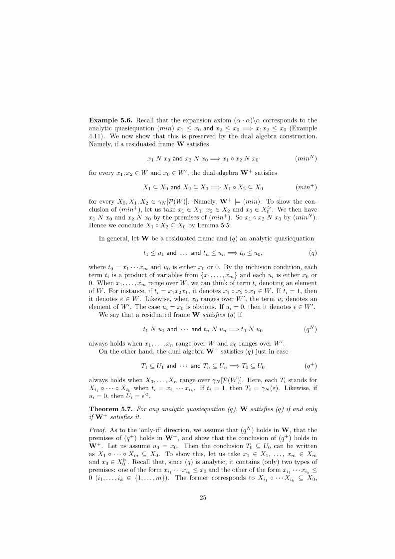
Example 5.6. Recall that the expansion axiom (α · α)\α corresponds to theanalytic quasiequation (min) x1 ≤ x0 and x2 ≤ x0 =⇒ x1x2 ≤ x0 (Example4.11). We now show that this is preserved by the dual algebra construction.Namely, if a residuated frame W satisfies

x1 N x0 and x2 N x0 =⇒ x1 ◦ x2 N x0 (minN )

for every x1, x2 ∈W and x0 ∈W ′, the dual algebra W+ satisfies

X1 ⊆ X0 and X2 ⊆ X0 =⇒ X1 ◦X2 ⊆ X0 (min+)

for every X0,X1,X2 ∈ γN [P(W )]. Namely, W+ |= (min). To show the con-clusion of (min+), let us take x1 ∈ X1, x2 ∈ X2 and x0 ∈ X⊲

0 . We then havex1 N x0 and x2 N x0 by the premises of (min+). So x1 ◦ x2 N x0 by (minN ).Hence we conclude X1 ◦X2 ⊆ X0 by Lemma 5.5.

In general, let W be a residuated frame and (q) an analytic quasiequation

t1 ≤ u1 and . . . and tn ≤ un =⇒ t0 ≤ u0, (q)

where t0 = x1 · · ·xm and u0 is either x0 or 0. By the inclusion condition, eachterm ti is a product of variables from {x1, . . . , xm} and each ui is either x0 or0. When x1, . . . , xm range over W , we can think of term ti denoting an elementof W . For instance, if ti = x1x2x1, it denotes x1 ◦ x2 ◦ x1 ∈ W . If ti = 1, thenit denotes ε ∈ W . Likewise, when x0 ranges over W ′, the term ui denotes anelement of W ′. The case ui = x0 is obvious. If ui = 0, then it denotes ǫ ∈W ′.

We say that a residuated frame W satisfies (q) if

t1 N u1 and · · · and tn N un =⇒ t0 N u0 (qN )

always holds when x1, . . . , xn range over W and x0 ranges over W ′.On the other hand, the dual algebra W+ satisfies (q) just in case

T1 ⊆ U1 and · · · and Tn ⊆ Un =⇒ T0 ⊆ U0 (q+)

always holds when X0, . . . ,Xn range over γN [P(W )]. Here, each Ti stands forXi1 ◦ · · · ◦ Xik

when ti = xi1 · · ·xik. If ti = 1, then Ti = γN (ε). Likewise, if

ui = 0, then Ui = ǫ⊳.

Theorem 5.7. For any analytic quasiequation (q), W satisfies (q) if and onlyif W+ satisfies it.

Proof. As to the ‘only-if’ direction, we assume that (qN ) holds in W, that thepremises of (q+) holds in W+, and show that the conclusion of (q+) holds inW+. Let us assume u0 = x0. Then the conclusion T0 ⊆ U0 can be writtenas X1 ◦ · · · ◦ Xm ⊆ X0. To show this, let us take x1 ∈ X1, . . . , xm ∈ Xm

and x0 ∈ X⊲

0 . Recall that, since (q) is analytic, it contains (only) two types ofpremises: one of the form xi1 · · ·xik

≤ x0 and the other of the form xi1 · · ·xik≤

0 (i1, . . . , ik ∈ {1, . . . ,m}). The former corresponds to Xi1 ◦ · · ·Xik⊆ X0,

25

and the latter to Xi1 ◦ · · ·Xik⊆ ǫ⊳ in (q+). Since we assume all premises of

(q+), Lemma 5.5 yields xi1 · · ·xikN x0 for the former and xi1 · · ·xik

N ǫ forthe latter. Namely, all premises of (qN ) hold. So we obtain t0 N u0 by (qN ),namely x1◦· · ·◦xm N x0. Since this holds for every x1 ∈ X1, . . . , xm ∈ Xm andx0 ∈ X⊲

0 , we conclude that X1 ◦ · · · ◦Xm ⊆ X0 by Lemma 5.5. The argumentis similar and easier when u0 = 0.

As to the ‘if’ direction, suppose that x1, . . . , xn range over W and x0 overW ′ in (qN ). We consider the instantiation X1 = γN ({x1}), . . . ,Xm = γN ({xm})and X0 = x⊳

0 in (q+). Under this instantiation, we have ti N ui iff Ti ⊆ Ui byLemma 5.5. Hence whenever (q+) holds in W+, (qN ) holds in W.

Remark 5.8. The linearity condition for (q) (see Definition 4.3) is essentialfor the above argument to go through. To see this, consider a non-analyticquasiequation (q) x1x1x1 ≤ x0 =⇒ x1x1 ≤ x0. Let us try to derive from thecondition (qN ) on W

x1 ◦ x1 ◦ x1 N x0 =⇒ x1 ◦ x1 N x0, (qN )

the condition (q+) in W+

X1 ◦X1 ◦X1 ⊆ X0 =⇒ X1 ◦X1 ⊆ X0. (q+)

To prove the conclusion X1 ◦X1 ⊆ X0, it is natural to take x1 ∈ X1, x2 ∈ X1

and x0 ∈ X⊲

0 and try to show x1 ◦ x2 N x0 by using (qN ). However, the latterdoes not match the conclusion of (qN ), hence the argument breaks down. Thisis the reason why we impose the linearity condition on analytic quasiequations(see also [41] and [22] for the need of linearity for cut-elimination).

5.3. Gentzen frames

The dual algebra construction produces a complete FL-algebra W+ from agiven residuated frame W so that analytic quasiequations are transferred. Itremains to show that there exists a suitable (quasi)homomorphism f into W+,provided that W satisfies the rules of the sequent calculus FL. For ‘cut-free’W, this quasihomomorphism is indeed the algebraic essence of cut-elimination.When W further satisfies ‘cut,’ f gives rise to an embedding associated to theMacNeille completion.

We begin by making clear what it means for a frame to satisfy the rules ofthe sequent calculus. We denote by L the language of FL. An L-algebra issimply an algebra over the language L. It does not need to be an FL-algebra;typically, the set Fm of all formulas forms an L-algebra Fm.

Definition 5.9. A Gentzen frame is a pair (W,A) where

• W = (W,W ′, N, ◦, ε, ǫ) is a residuated frame, A is an L-algebra,

• there are injections ι : A −→ W and ι′ : A −→ W ′ (under which we willidentify A with a subset of W and a subset of W ′),

26

x N a a N zx N z

(CUT)a N a

(Id)

x N a b N za\b N x z

(\L)x N a b

x N a\b(\R)

x N a b N zb/a N z�x

(/L)x N b�a

x N b/a(/R)

a ◦ b N za · b N z

(·L)x N a y N b

x ◦ y N a · b(·R)

a N za ∧ b N z

(∧Lℓ) b N za ∧ b N z

(∧Lr) x N a x N bx N a ∧ b

(∧R)

a N z b N za ∨ b N z

(∨L) x N ax N a ∨ b

(∨Rℓ) x N bx N a ∨ b

(∨Rr)

ε N z1 N z

(1L)ε N 1

(1R)0 N ǫ

(0L) x N ǫx N 0

(0R)

Figure 5: Gentzen rules

• N satisfies the Gentzen rules (or rather conditions) of Figure 5 for alla, b ∈ A, x, y ∈W and z ∈W ′.

A cut-free Gentzen frame is defined in the same way, but it is not stipulatedto satisfy the (CUT) rule.

Example 5.10. If A is an FL-algebra, then the pair (WA,A) is a Gentzenframe (see Example 5.2).

(WFL,Fm) is also a Gentzen frame, while (WcfFL,Fm) is a cut-free Gentzen

frame (see Example 5.3). To see this, notice that the conditions (\L) and (\R)can be equivalently expressed by

x N a b N zx ◦ a\b N z

a ◦ x N bx N a\b .

Now, recall that in WFL every x ∈ W is a sequence Σ of formulas and everyz ∈W ′ is a pair ((Γ, ,∆),Π). Hence the above two rules mean

Σ ⇒ α Γ, β,∆ ⇒ Π

Γ,Σ, α\β,∆ ⇒ Π

α,Σ ⇒ β

Σ ⇒ α\β,

which precisely correspond to the inference rules for \.

Given two L-algebras A and B, a quasihomomorphism from A to B is afunction F : A −→ P(B) such that

cB ∈ F (cA) for c ∈ {0, 1},F (a) ⋆B F (b) ⊆ F (a ⋆A b) for ⋆ ∈ {·, \, /,∧,∨}, a, b ∈ A,

27

where X ⋆B Y = {x ⋆B y|x ∈ X, y ∈ Y } for any X,Y ⊆ B.It is equivalent to the standard notion of homomorphism when F (a) is a

singleton for every a ∈ A. The theorem below provides us with a suitable(quasi)homomorphism to the dual algebra.

Theorem 5.11 ([19]).

1. If (W,A) is a cut-free Gentzen frame, then

F (a) = {X ∈ γN [P(W )] : a ∈ X ⊆ a⊳}

is a quasihomomorphism from A to W+.

2. If (W,A) is a Gentzen frame, then f(a) = a⊲⊳ = a⊳ is a homomorphismfrom A to W+. Moreover, f is an embedding when N is antisymmetric.

Proof. 1. We verify the conditions on F for ⋆ ∈ {∧, \}, referring to [19] for theremaining cases. Let a, b ∈ A, X ∈ F (a) and Y ∈ F (b), namely,

a ∈ X ⊆ a⊳, b ∈ Y ⊆ b⊳.

(Case ⋆ = ∧) First, we have X ∩ Y ⊆ a⊳ ∩ b⊳ ⊆ (a ∧ b)⊳, where the the lastinclusion is due to the rule (∧R) of Figure 5. Second, observe that a ∈ X impliesa ∧ b ∈ X. Indeed, if z ∈ X⊲ we have a N z, so a ∧ b N z by the rule (∧Lℓ).This proves a ∧ b ∈ X⊲⊳ = X. Similarly, a ∧ b ∈ Y . We have thus established

a ∧ b ∈ X ∩ Y ⊆ (a ∧ b)⊳,

namely X ∧W+ Y ∈ F (a ∧A b).(Case ⋆ = \) Let x ∈ X\Y . Since a ∈ X and Y ⊆ b⊳, we have a ◦ x ∈ Y ⊆ b⊳.So a ◦ x N b, which implies x N a\b by the rule (\R), i.e., x ∈ (a\b)⊳. Thisproves X\Y ⊆ (a\b)⊳. To show a\b ∈ X\Y , let x ∈ X and z ∈ Y ⊲. SinceX ⊆ a⊳ and b ∈ Y , we have x N a and b N z. Hence by the rule (\L), we havea\b N x z, i.e. x ◦ a\b N z. Since this holds for every x ∈ X and z ∈ Y ⊲, weconclude X ◦{a\b} ⊆ Y ⊲⊳ = Y . Namely, a\b ∈ X\Y . We have thus established

a\b ∈ X\Y ⊆ (a\b)⊳,

namely X\W+Y ∈ F (a\Ab).

2. From the (Id) rule follows a ∈ a⊳, so a⊲⊳ ⊆ a⊳. We also have a⊳ ⊆ a⊲⊳.To show this, let x ∈ a⊳, so x N a. For every z ∈ a⊲, we have a N z, so x N zby (CUT). Namely x ∈ a⊲⊳. As a consequence,

F (a) = {X ∈ γN [P(W )] : a⊲⊳ ⊆ X ⊆ a⊳} = {a⊲⊳},

hence F boils down to a homomorphism.Suppose that N is antisymmetric and f(a) = f(b). We then have a ∈ b⊲

and b ∈ a⊲. Namely, a N b and b N a, so a = b. This proves that f is anembedding.

28

5.4. Preservation by MacNeille completions

We already have enough facts to conclude that analytic quasiequations arepreserved by MacNeille completions. But before that, let us observe a generalfact that preservation under completions implies conservativity with respect toinfinitary extensions.

More precisely, let κ be a cardinal. We enrich the set of formulas so thatboth

∧

i∈I αi and∨

i∈I αi are formulas if αi is a formula for every i ∈ I, whereI is an arbitrary index set with |I| ≤ κ. We also add the following inferencerules:

Γ1, αi,Γ2 ⇒ Π for some i ∈ I

Γ1,∧

i∈I αi,Γ2 ⇒ Π(∧l)

Γ ⇒ αi for all i ∈ I

Γ ⇒∧

i∈I αi

(∧r)

Γ1, αi,Γ2 ⇒ Π for all i ∈ I

Γ1,∨

i∈I αi,Γ2 ⇒ Π(∨l)

Γ ⇒ αi for some i ∈ I

Γ ⇒∨

i∈I αi

(∨r)

The extension of FLR with these infinitary connectives is denoted by FLκR.

Notice that the cardinality restriction on I is necessary, since otherwise thecollection of formulas would constitute a proper class.

Definition 5.12. Let R be a set of structural rules and κ a cardinal. We saythat FLκ

R is a conservative extension (atomic conservative extension, resp.) ofFLR if S ⊢FLκ

Rs implies S ⊢FLR

s, whenever S is a set of sequents (resp. atomicsequents), and s is a sequent in the language of FL. Here an atomic sequent isa sequent that consists of atomic formulas.

Recall that a completion of an algebra A is a complete algebra B togetherwith an embedding ι : A −→ B. We often identify A with ι[A] and do notmention the embedding ι explicitly. We say that a class K of algebras admitscompletions if every A ∈ K has a completion in K. The following is a generalfact, although we only state it for FL with structural rules.

Lemma 5.13. Let R be a set of structural rules and R• the set of quasiequationsinterpreting them (cf. Section 2.5). If FLR• admits completions, then FLκ

R is aconservative extension of FLR for every cardinal κ.

Proof. Assume S ⊢FLκRs. In view of the algebraization of FL (subsection 2.4),

it suffices to show that ε[S] |=A ε(s) holds for every algebra A ∈ FLR• . Byassumption, A has a completion A′ in FLR• . Since all rules of FLκ

R, includingthe rules for

∧and

∨, are sound in A′, we have ε[S] |=A′ ε(s). Since A is

(isomorphic to) a subalgebra of A′, ε[S] |=A ε(s).

Completions of a given algebra are not unique in general. Among them, ourframe-based construction yields a particularly important one.

Definition 5.14. Given an FL-algebra A, a completion ι : A −→ B is called aMacNeille completion if ι[A] is both join-dense and meet-dense in B. Namely,for every element x ∈ B there exist P,Q ⊆ ι[A] such that x =

∨P =

∧Q.

29

MacNeille completions of A are unique up to isomorphisms that fix A (cf.[5, 38]), hence we usually speak of the MacNeille completion.

Proposition 5.15. Given an FL-algebra A, W+A

is the MacNeille completionof A.

Proof. W+A

is a complete FL-algebra by Lemma 5.4. Since (WA,A) is aGentzen frame with N antisymmetric, f(a) = γN (a) = a⊲⊳ = a⊳ is an em-bedding from A to W+

Aby Theorem 5.11. Recall that every element of W+

Ais

a set X ⊆ A such that X = X⊲⊳. We have

X =⋃

γN{γN (a) : a ∈ X} =

∨{f(a) : a ∈ X},

=⋂{a⊳ : a ∈ X⊲} =

∧{f(a) : a ∈ X⊲}.

The first line follows from the properties of nuclei. For the second line, observe

b ∈ X ⇐⇒ b ∈ X⊲⊳

⇐⇒ b N a for every a ∈ X⊲

⇐⇒ b ∈⋂

{a⊳ : a ∈ X⊲}.

This proves join-density and meet-density.

A notable feature of the MacNeille completion is that it preserves all exist-ing joins and meets. Hence it is useful when proving the completeness theoremfor predicate substructural logics with respect to the associated classes of com-plete FL-algebras (see [34]). We refer to [42] for a general study of MacNeillecompletions for arbitrary lattice expansions.

Notice that an FL-algebra A satisfies an analytic quasiequation (q) if andonly if WA satisfies it. Hence a direct consequence of Theorem 5.7 is thefollowing:

Theorem 5.16. Analytic quasiequations are preserved by MacNeille comple-tions. Namely, if A satisfies an analytic quasiequation (q), then W+

Aalso sat-

isfies (q).

Corollary 5.17. If E is a set of acyclic N2-equations, the variety FLE of FL-algebras satisfying E admits MacNeille completions, and FLκ

E is a conservativeextension of FLE for every cardinal κ.

5.5. Strong analyticity

Turning to the proof-theoretic side, we will give an algebraic proof of cut-elimination for FL extended with a set R of analytic structural rules. Actually,we prove a stronger form of cut-elimination which we call strong analyticity, andmoreover not just for finitary systems, but also for arbitrary infinitary extensionsof FLR. Roughly speaking, strong analyticity refers to a property that cut rulescan be eliminated from a given derivation with nonlogical atomic assumptions,and the resulting cut-free derivations satisfy the subformula property, i.e. theyconsist of formulas already contained in the statements to be proved. Here we

30

need to mention the subformula property explicitly, since a system that admitscut-elimination might not satisfy the subformula property due to some peculiarstructural rules.

Informally, a semantic proof of cut-elimination proceeds as follows:

⊢ ϕ =⇒ A |= ϕ and A |= ϕ =⇒ ⊢cut−free ϕ

⊢ ϕ =⇒ ⊢cut−free ϕ ,

where the first premise is the soundness of the semantics and the second premiseis the cut-free completeness. Of course, the crucial step of this argument is tobuild a suitable semantic model A which is sound with respect to derivability⊢ on the one hand, and is intensionally associated to the cut-free derivability⊢cut−free on the other hand. In our setting, this is achieved by the dual algebraconstruction from a cut-free Gentzen frame (Lemma 5.4) and the quasihomo-morphism given by Theorem 5.11.

Let us now proceed to the formal argument.

Definition 5.18. A set S of sequents is said to be elementary if S consists ofatomic sequents and is closed under cuts: if S contains Σ ⇒ p and Γ, p,∆ ⇒ Π,it also contains Γ,Σ,∆ ⇒ Π.

A sequent calculus is strongly analytic if for any elementary set S and asequent s in the finitary language, if s is derivable from S, then s has a cut-freederivation from S in which only subformulas of formulas in s occur.

Strong analyticity subsumes cut admissibility and subformula property inthe usual sense (by taking S = ∅). We also use this concept for infinitarysystems FLκ

R, but notice that the conclusion sequent s is restricted to the finitarylanguage, i.e., it does not contain infinitary

∧or

∨.

A direct consequence of strong analyticity is atomic conservativity with re-spect to infinitary extensions.

Lemma 5.19. Let R be a set of structural rules and κ a cardinal. If FLκR is

strongly analytic, then FLκR is an atomic conservative extension of FLR.

Proof. Let S be a set of atomic sequents, s a sequent in the language of FL andsuppose that S ⊢FLκ

Rs. Then we have S0 ⊢FLκ

Rs, where S0 is the closure of S

under cuts; note that S0 is elementary. By strong analyticity s has a cut-freederivation from S0 obeying the subformula property. Hence S0 ⊢FLR

s, sinces is in the language of FL. Since all sequents in S0 are derivable from S, weconclude S ⊢FLR

s.

We now prove strong analyticity of FLκR, where R is a set of analytic rules.

The first thing to do is to build a suitable frame, that is analogous to WcfFL

ofExample 5.3.

Given an elementary set S, we define a frame WR,S = (W,W ′, N, ◦, ε, ǫ) asfollows:

• (W, ◦, ε) is the free monoid generated by Fm,

31

• W ′ = SW × (Fm ∪ {ǫ}),

• Σ N (C,Π) iff C = (Γ, ,∆) and Γ,Σ,∆ ⇒ Π is cut-free derivable from Sin FLR.

For the next lemma, our specific way of reading back a structural rule (q◦)from an analytic quasiequation (q) is crucial.

Lemma 5.20. (WR,S ,Fm) is a cut-free Gentzen frame. Moreover, W+R,S

satisfies the quasiequations in R•.

Proof. The first claim is easily verified as in Example 5.10. For the second claim,we have to verify that W+

R,S satisfies the quasiequation (r•) for each analyticrule (r) ∈ R. Since the general case is tedious, let us consider one examplewhich is general enough to grasp the idea. Suppose that (r) is

Σ1 ⇒ Γ,Σ2,Σ2,∆ ⇒ Π

Γ,Σ1,Σ2,∆ ⇒ Π(r).

(r) arises from the analytic quasiequation

x1 ≤ 0 and x2x2 ≤ x0 =⇒ x1x2 ≤ x0 (q)

so that (r) = (q◦). We claim that WR,S satisfies (q), namely

x1 N ǫ and x2 ◦ x2 N x0 =⇒ x1 ◦ x2 N x0 (qN )

holds when x1, x2 range over W and x0 over W ′. Since xi ∈ W is of the formΣi for i = 1, 2 and x0 ∈ W ′ is of the form ((Γ, ,∆),Π), (qN ) amounts to thefollowing:

• If Σ1 ⇒ and Γ,Σ2,Σ2,∆ ⇒ Π are cut-free derivable from S in FLR,then so is Γ,Σ1,Σ2,∆ ⇒ Π.

This certainly holds as the rule (r) ∈ R.Therefore, W+

R,S satisfies (q) by Theorem 5.7. Notice that the quasiequation(q) is equivalent to (q◦•) by Lemma 4.8, which is in turn equivalent to (r•) bydefinition. Therefore W+

R,S satisfies (r•).

We next define a valuation into W+R,S which makes all sequents in S true,

so that the soundness argument goes through. For each propositional variablep, let

S(p) = {Γ : Γ ⇒ p ∈ S} ∪ {p}

and define a valuation f by f(p) = γN (S(p)) and homomorphically extending itto all formulas. Given a sequent s, we say that s is true under f if |=

W+R,S

,f ε(s).

This holds when f(α1) ◦ · · · ◦ f(αm) ⊆ f(β) if s is of the form α1, . . . , αm ⇒ β,and when f(α1) ◦ · · · ◦ f(αm) ⊆ ǫ⊳ if s is of the form α1, . . . , αm ⇒ .

Lemma 5.21. For any formula α, α ∈ f(α) ⊆ α⊳. Moreover, all sequents inS are true under f .

32

Proof. For every propositional variable p, we have p ∈ S(p) ⊆ p⊳, hence p ∈f(p) ⊆ p⊳. Since the function F (α) = {X ∈ γN [P(W )] : α ∈ X ⊆ α⊳} is aquasi-homomorphism from Fm to W+

R,S by Theorem 5.11, we can inductivelyshow that α ∈ f(α) ⊆ α⊳ for every formula α.

To verify the second claim for a sequent of the form p1, . . . , pn ⇒ q inS, let Γ1 ∈ S(p1), . . . ,Γn ∈ S(pn). Since S is closed under cuts, we haveΓ1, . . . ,Γn ⇒ q in S. This shows that S(p1) ◦ · · · ◦ S(pn) ⊆ S(q), and hencef(p1) ◦ · · · ◦ f(pn) ⊆ f(q).

For a sequent of the form p1, . . . , pn ⇒ in S, let Γ1 ∈ S(p1), . . . ,Γn ∈S(pn). Since S is closed under cuts, Γ1, . . . ,Γn ⇒ belongs to S, we haveS(p1) ◦ · · · ◦ S(pn) ⊆ ǫ⊳, and hence f(p1) ◦ · · · ◦ f(pn) ⊆ f(0).

We are now ready to prove:

Theorem 5.22. If R is a set of analytic structural rules, FLκR is strongly

analytic for every cardinal κ.

Proof. Suppose that a sequent s of the form α1, . . . , αm ⇒ β is derivable froman elementary set S in FLκ

R (the case of α1, . . . , αm ⇒ is similar). We build aresiduated frame WR,S and a valuation f as described above. Then all sequentsin S are true under f by Lemma 5.21 and all inference rules of FLκ

R are soundin W+

R,S , since W+R,S is a complete FL-algebra (thus admitting interpretations

of∧

,∨

) and satisfies all structural rules in R by Lemma 5.20. Therefore, wehave f(α1) ◦ · · · ◦ f(αm) ⊆ f(β). Hence

α1, . . . , αm ∈ f(α1) ◦ · · · ◦ f(αm) ⊆ f(β) ⊆ β⊳,

which means that s is cut-free derivable from S in FLR.The subformula property is obvious, given that all structural rules are ana-

lytic, and thus satisfy the inclusion condition.

Remark 5.23. In defining strong analyticity, the conclusion sequent s waslimited to be in the language of FL (i.e. without

∧,

∨). This restriction,

which greatly simplified our proofs, is however inessential, and indeed it can beremoved by suitably modifying the definition of cut-free Gentzen frames.

6. Closing the Cycle

Our achievements so far may be illustrated as follows:

33

Acyclicity

Theorem 4.5

Analyticity

Theorem 5.22 Theorem 5.16

Strong analyticity MacNeille completion

Lemma 5.19 Lemma 5.13

Atomic Conservativity

Here we close the cycle by showing that atomic conservativity (with κ = ω) im-plies analyticity, that is if FLω

R is an atomic conservative extension of FLR thenR is equivalent to a set of analytic structural rules. Since the argument belowis of a proof-theoretic nature, we first explain the idea in terms of structuralrules.

Example 6.1. Consider the rule

α, β ⇒ β

β, α⇒ β(we)

.

Let R0 be a set of structural rules and R = R0 ∪ {(we)}. Assume that FLωR

is an atomic conservative extension of FLR. Although (we) is not acyclic, weclaim that it is equivalent to an analytic rule in presence of the other rules inR0.

First of all, note that (we) is equivalent to

α, β ⇒ β γ ⇒ β β ⇒ δ

γ, α⇒ δ(we′)

by the restructuring step in Section 4.1 (see also Lemma 3.4). Let a, c, d bepropositional variables, and b the infinitary formula

∨

0≤n anc. Let S be the set

{a(k), c⇒ d : 0 ≤ k}. Now, observe that we have

⊢FLω a, b⇒ b, ⊢FLω c⇒ b, and S ⊢FLω b⇒ d,

corresponding to the three premises of (we′). Hence we have S ⊢FLωRc, a ⇒ d

by (we′). By the assumption of atomic conservativity, S ⊢FLRc, a ⇒ d. Since

a derivation in FLR is always finite, there must be an n such that c, a ⇒ d isderivable from Sn = {a(k), c⇒ d : 0 ≤ k ≤ n}.

Now we claim that R is equivalent to R0 with the following rule:

γ ⇒ δ α, γ ⇒ δ α(2), γ ⇒ δ . . . α(n), γ ⇒ δ

γ, α⇒ δ(we′′)

34

It is clear that (we′′) implies (we′) because the premises of the latter imply allthe premises of the former. On the other hand, we have a derivation of theconclusion of (we′′) from the premises in FLR; it can be easily obtained fromthe derivation of c, a⇒ d from Sn. This means that R implies (we′′).

Notice that (we′′) is acyclic, hence it can be transformed into an equivalentanalytic rule by the procedure described in Section 4.

The above argument can be generalized. Hence we have:

Theorem 6.2. Let R be a set of structural rules. If FLωR is an atomic con-

servative extension of FLR, then R is equivalent to a set of analytic structuralrules.

Proof. We argue in terms of algebra. LetQ be a set of structural quasiequations.We prove that Q is equivalent to a set of analytic quasiequations under theassumption of atomic conservativity: E |=FLω

Qε implies E |=FLQ

ε whenever

E ∪ {ε} is a set of equations of the form y1 . . . ym ≤ y0 or y1 . . . ym ≤ 0. Here,FL

ωQ consists of algebras in FLQ in which all countable joins and meets exist.Given a non-analytic quasiequation in Q, we apply the analytic completion

procedure in Section 4.1 with slight modifications. First, we can apply therestructuring step without any problem to obtain a quasiequation (q). As tothe cutting step, let z be a redundant variable in (q) and suppose that z occursboth in the RHS and LHS of premises (otherwise the procedure is just as before).

We classify the premises of (q) into four groups:

• SR = {si ≤ z : 1 ≤ i ≤ k}, which have z only in the RHS.

• SL = {tj(z, . . . , z) ≤ uj : 1 ≤ j ≤ l}, which have z only in the LHS.

• SM = {vj(z, . . . , z) ≤ z : 1 ≤ j ≤ m}, which have z in both.

• SO, the others.

Let T be the least set of terms such that

• si ∈ T for 1 ≤ i ≤ k,

• if w1, . . . , wn ∈ T , then vj(w1, . . . , wn) ∈ T for 1 ≤ j ≤ m.

Let also

S′L = {tj(w1, . . . , wn) ≤ uj : 1 ≤ j ≤ l, w1, . . . , wn ∈ T}.

We claim that S′L ∪ SO |=FLω

Qε, where ε is the conclusion of (q). To show this,

we consider the instantiation z =∨T , which makes sense as countable joins

and meets exist in all algebras in FLωQ. All equations in SR hold under this

instantiation and those in SM hold too, because

vj(∨

T, . . . ,∨

T ) =∨

vj(w1, . . . , wm) ≤∨

T,

35

with w1, . . . , wm ∈ T . Moreover, the equations in SL under the instantia-tion follow from S′

L. This shows that S′L ∪ SO |=FLω

Qε, being z a redundant

variable (i.e. z does not appear in the conclusion). By atomic conservativityS′

L ∪ SO |=FLQε, and by compactness, there is a finite subset S′′

L ⊆ S′L such

that S′′L ∪ SO |=FLQ

ε. Let (q′) be the quasiequation corresponding to the latterconsequence relation. So, Q implies (q′).

Conversely (q′) implies (q) by transitivity. Hence one can replace (q) inQ by (q′). The number of redundant variables is decreased by one. Henceby repeating this process, we obtain an analytic quasiequation equivalent to(q).

Let us summarize what we have achieved:

Theorem 6.3.

1. Every N2-axiom/equation is equivalent to a set of structural rules/quasiequations.

2. For any set R of structural rules, the following are equivalent:

• R is equivalent to a set of acyclic structural rules.

• R is equivalent to a set of analytic structural rules.

• R• is preserved by MacNeille completions.

• FLκR is a conservative extension of FLR for every κ.

• R is equivalent to R′ such that FLκR′ is strongly analytic for every κ.

If R implies left weakening (i), all the above hold.

3. For any set E of N2-equations, the following are equivalent:

• E is equivalent to a set of acyclic quasiequations.

• E is equivalent to a set of analytic quasiequations.

• The variety FLE admits MacNeille completions.

• FLE admits completions.

If E implies integrality x ≤ 1, all the above hold.

It follows that strong analyticity for infinitary extensions FLκR is equiva-

lent to admitting completions as far as N2 axioms/equations and structuralrules/quasiequations are concerned (actually strong analyticity of FLω

R is enough).Also notably, MacNeille completions are optimal for the subvarieties of FL de-fined by N2-equations: if such a subvariety admits completions, it necessarilyadmits MacNeille completions.

We end this section showing the existence of a structural rule/N2-equationwhich does not satisfy any of conditions (2) and (3) of the above theorem.Our proof below exhibits a real interplay between proof-theoretic and algebraicarguments.

Proposition 6.4. Not all N2-equations are equivalent to acyclic quasiequations.

36

Proof. Consider the equation y/y ≤ y\y and denote it by ε. ε is easily seen tobe equivalent to

xy ≤ y =⇒ yx ≤ y, (we•)

which is an interpretation of the rule (we) in Example 6.1. If (we) is equivalentto an acyclic rule, then FLω

(we) is conservative over FL(we) by Theorem 6.3.Hence by the argument in Example 6.1, (we) is equivalent to a rule of the form

γ ⇒ δ α, γ ⇒ δ α(2), γ ⇒ δ . . . α(n), γ ⇒ δ

γ, α⇒ δ(we′′)

So, we have{pnq ≤ v : n ∈ ω} |=FLε

qp ≤ v.

We will show that this is not the case, by exhibiting an algebra A in FLε

and elements a, b, c ∈ A such that anb ≤ c for all n ∈ ω, but ba 6≤ c.The equation ε is satisfied by all lattice-ordered groups, since y/y = yy−1 =

1 = y−1y = y\y. We can take as A the totally ordered ℓ-group based on the freegroup on two generators, constructed in [7]; it is shown there that A satisfiesthe property: if 1 ≤ xm ≤ y, for all m ∈ ω, then xm ≤ y−1xy, for all m ∈ ω.Since the ℓ-group is based on the free group on two generators, it is not Abelian.Moreover, since it is totally ordered there exist elements g, h ∈ A with 1 < g, hand gm < h, for all m ∈ ω; otherwise the ℓ-group would be archimedean, andevery totally ordered archimedean ℓ-group is abelian. By the property of theconstructed ℓ-group, we get gm ≤ h−1gh, namely gmh−1 ≤ h−1g, for all m ∈ ω.Now, let a = g2, b = h−1, and c = h−1g. We have anb = g2nh−1 ≤ h−1g = c,for all n ∈ ω; but c = h−1g < h−1g2 = ba, because 1 < g, so ba 6≤ c.

Remark 6.5. The same holds for the system FL⊥. Since ℓ-groups are not inFL⊥, we have to slightly modify the above argument. We consider the aboveℓ-group and we add two new elements ⊥, below every element, and ⊤, aboveevery element. Multiplication is extended so that ⊤ is an absorbing element forA∪ {⊤} and ⊥ is an absorbing element for A∪ {⊤,⊥}. It is shown in [23] thatthis construction yields an FL-algebra into which A embeds. Moreover, it iseasy to see that it satisfies y/y ≤ y\y, as ⊤/⊤ = ⊤\⊤ = ⊤ = ⊥/⊥ = ⊥\⊥.

The above proposition shows the limitations of strong analyticity and Mac-Neille completions within the class N2.

7. Expressive Power of Structural Rules

Each N2-equation can be transformed into equivalent structural quasiequa-tions and hence into structural rules (Theorem 3.5). This shows what struc-tural rules can express. In this section we address the converse problem, namelyidentifying which properties (equations over residuated lattices, or equivalently,Hilbert axioms in the language of FL⊥) cannot be expressed by structural rules.

The proposition below, which easily follows from our analytic completion,essentially says that the expressive power of structural rules cannot go beyondintuitionistic logic.

37

Proposition 7.1. Any structural rule (r) is either derivable in Gentzen’s LJ

or derives in LJ every formula (i.e., LJ(r) is contradictory).

Proof. We first apply our analytic completion procedure to obtain, by Theorem4.9, an analytic rule (r′) equivalent to (r) in LJ (this is always possible inpresence of the left weakening rule (i)). Two cases can arise. If (r′) has nopremises, any formula is derivable in LJ extended with (r′) (and hence with (r)),as the LHS and the RHS of the conclusion of (r′) are disjoint. Otherwise, theconclusion of (r′) is derivable from any of its premises by weakening, exchangeand contraction due to the separation and inclusion conditions of Definition4.6.

Hence structural rules added to LJ do not define any proper consistentsuperintuitionistic logic.

Remark 7.2. Our proof theoretic limitation is in accordance with the limit es-tablished in [8] for MacNeille completions for the variety HA of Heyting algebras:there are only three subvarieties of HA closed under MacNeille completions, thatis the trivial variety, the whole variety HA, and the variety BA of Boolean alge-bras. The small mismatch on Boolean algebras is due to the fact that we restricthere to single conclusion sequent calculi: there is of course a multiple conclu-sion sequent calculus that captures BA, that is Gentzen’s LK. See [13] for aproof-theoretic analysis of the substructural hierarchy, adapted to commutativemultiple conclusion (hyper)sequent calculi.

The limitations of structural rules are however stronger. Indeed, as shownbelow, even among the properties which do hold in intuitionistic logic (Heytingalgebras), only some can be captured by structural sequent rules.

Proposition 7.3. Any equation equivalent to a structural rule is preserved byMacNeille completions in presence of integrality.

Proof. Let (q) be the equivalent structural quasiequation. Theorem 4.9 ensuresthat, in presence of integrality x ≤ 1, (q) is equivalent to a set Q of analyticquasiequations. By Theorem 5.16, Q is preserved by MacNeille completions.

As a particular case we have

Corollary 7.4. No structural rule is equivalent to the distributivity axiom.

Proof. We use Proposition 7.3 and the fact that distributivity is not preservedby MacNeille completions, even in presence of integrality. To see this, consider abounded distributive lattice L whose MacNeille completion L is not distributive;such a lattice was constructed in [10]. It easy to see that the ordinal sumL ⊕ {1} (obtained by adding a new top element 1 to L) supports a residuatedlattice structure, by defining multiplication as xy = ⊥, for x, y ∈ L and setting1 as the unit element. The MacNeille completion of the integral distributiveresiduated lattice L⊕{1} is clearly the ordinal sum L⊕{1}, which also fails tobe distributive.

38

In contrast to the negative results above, it follows from our analytic comple-tion that all “natural” structural rules can be expressed by N2-axioms (Corollary7.6 below).

Proposition 7.5. Any analytic quasiequation without any premise 1 ≤ 0 isequivalent to an N2 equation.

Proof. Suppose that the conclusion is of the form x1 · · ·xm ≤ x0 (the casex1 · · ·xm ≤ 0 is similar). Let t1 ≤ x0, . . . , tn ≤ x0 be the premises having x0 inthe RHS, and s1 ≤ 0, . . . , sk ≤ 0 the others. By assumption1 each si is not 1,hence one can pick up a ‘pivot’ xj for some 1 ≤ j ≤ m (cf. Proposition 3.11)and write si = lixjri. Define a substitution σ by

σ(x0) = t1 ∨ · · · ∨ tn,σ(xj) =

∧li\0/ri, for 1 ≤ j ≤ m,

where the meet∧li\0/ri is built from those premises lixjri ≤ 0 for which xj

has been chosen as pivot. It is easy to see that σ is a solution. Hence it providesan equivalent equation by Proposition 3.10, that is easily shown to be N2.

Corollary 7.6. Let (r) be any analytic structural rule. If (r) does not containany empty premise ⇒ , then (r) is equivalent to an N2-axiom.

Hence we can reasonably claim that the expressive power of structural rulesis essentially limited to N2.

Concluding Remark: Beyond N2

Our main theorem shows that within the class N2 an equation is preservedunder MacNeille completions if and only if the corresponding sequent calculusstructural rule is analytic. This correspondence does not hold anymore outsidethe class N2 as witnessed by ¬¬x ≤ x (involutivity), which belongs to the classN3. The equation is preserved under MacNeille completions, but it does notcorrespond to any structural rule by Proposition 7.1.

Having explored the level N2 rather in depth, our next target are P2 andP3. Indeed, consider the prelinearity axiom (see Figure 3). By Proposition 7.1it cannot be expressed by any structural rule, as it is neither derivable in LJ

nor contradicts LJ. Since prelinearity belongs to P2, we have:

Corollary 7.7. There is an equation in P2 which is not equivalent to anyequation in N2.

This implies that the inclusions N2 ⊆ P3 and N2 ⊆ N3 are proper. It isleft open whether all inclusions in the substructural hierarchy (see Figure 4) areproper or not.

1The presence of a premise 1 ≤ 0 often leads to the non-existence of an equivalent equation,see Remark 3.8.

39

Notice that prelinearity can instead be expressed as a structural rule inhypersequent calculus – a simple generalization of sequent calculus whose addi-tional machinery is basically adding one more disjunction on top of sequents [2].In [12] we proved that in the commutative case, all axioms in the class P ′

3 (aslight modification of P3) can be expressed as structural rules in hypersequentcalculus which preserve cut admissibility. The recent paper [11] also shows thatall equations in P ′

3 are preserved by MacNeille completions when applied tosubdirectly irreducible algebras. In our subsequent work, we consider the gen-eral noncommutative case and perform a simultaneous investigation of (strong)analyticity in hypersequent calculi and closure under suitable completions forarbitrary FL-algebras extended by P3-equations.

References

[1] J.-M. Andreoli. Logic programming with focusing proofs in linear logic.Journal of Logic and Computation, 2(3):297–347, 1992.

[2] A. Avron. Hypersequents, logical consequence and intermediate logics forconcurrency. Annals of Mathematics and Artificial Intelligence, 4: 225–248,1991.

[3] A. Avron and O. Lahav, Kripke semantics for Basic Sequent Systems, Pro-ceedings of Tableaux 2011, LNCS 6793: 43-57, 2011.

[4] A. Avron and A. Zamansky, Non-deterministic Semantics for Logical Sys-tems, forthcoming in the Handbook of Philosophical Logic, 2011.

[5] B. Banaschewski. Hullensysteme und Erweiterungen von Quasi-Ordnungen.Z. Math. Logik Grund. Math., 2: 35-46, 1956.

[6] F. Belardinelli, P. Jipsen and H. Ono. Algebraic aspects of cut-elimination.Studia Logica, 77(2):209–240, 2004.

[7] G. Bergman. Specially ordered groups. Comm. Algebra, 12(19-20), 2315–2333, 1984.

[8] G. Bezhanishvili and J. Harding: MacNeille completions of Heyting alge-bras. The Houston J. of Math. 30(4): 937 952, 2004.

[9] S. Buss. An Introduction to Proof Theory. Handbook of Proof Theory,Elsevier Science, pp. 1–78, 1998.

[10] N. Funayama. On the completion by cuts of distributive lattices. Proc. Imp.Acad. Tokyo, 20:1–2, 1944.

[11] A. Ciabattoni, N. Galatos and K. Terui. MacNeille Completions of FL-algebras, Algebra Universalis, to appear.

[12] A. Ciabattoni, N. Galatos and K. Terui. From axioms to analytic rules innonclassical logics. Proceedings of LICS 2008, pp. 229 – 240, 2008.

40

[13] A. Ciabattoni, L. Strassburger and K. Terui. Expanding the realm of sys-tematic proof theory. Proceedings of CSL 2009, LNCS 5771: 163-178, 2009.

[14] A. Ciabattoni and K. Terui. Towards a semantic characterization of cut-elimination. Studia Logica, 82(1):95–119, 2006.

[15] W. Conradie, V. Goranko, and D. Vakarelov. Algorithmic correspondenceand completeness in modal logic I: The core algorithm SQEMA. LogicalMethods in Computer Science, 2(1:5), 2006.

[16] W. Conradie and A. Palmigiano. Algorithmic Correspondence and Canon-icity for Distributive Modal Logic. Annals of Pure and Applied Logic, toappear.

[17] M. Gehrke, J. Harding and Y. Venema. MacNeille completions and canon-ical extensions. Transactions of the American Mathematical Society, 358:573-590, 2006.

[18] N. Galatos, Minimal varieties of residuated lattices, Algebra Universalis52(2) (2005), 215-239.

[19] N. Galatos and P. Jipsen, Residuated frames with applications to decid-ability, Transactions of the AMS, to appear.

[20] N. Galatos, P. Jipsen, T. Kowalski and H. Ono. Residuated Lattices: analgebraic glimpse at substructural logics, Studies in Logics and the Founda-tions of Mathematics, Elsevier, 2007.

[21] N. Galatos and H. Ono. Algebraization, parameterized local deduction the-orem and interpolation for substructural logics over FL. Studia Logica,83:279-308, 2006.

[22] N. Galatos and H. Ono. Cut-elimination and strong separation for substruc-tural logics: an algebraic approach, Annals of Pure and Applied Logic, 161(2010), no. 9, 1097–1133.

[23] N. Galatos and J. Raftery. Adding involution to residuated structures. Stu-dia Logica, 77(2): 181-207, 2004.

[24] J. Harding. Completions of ordered algebraic structures: a survey. Proceed-ings of the International Workshop on Interval/Probabilistic Uncertaintyand Non-classical Logics. Advances in Soft Computing. Ono et. al. Eds,Springer, 46: 231–244, 2008.

[25] R. Hori, H. Ono and H. Schellinx. Extending intuitionistic linear logicwith knotted structural rules. Notre Dame Journal of Formal Logic, 35(2):219–242, 1994.

[26] P. Jipsen and C. Tsinakis. A survey of residuated lattices, Ordered AlgebraicStructures (J. Martinez, ed.), Kluwer Academic Publishers, Dordrecht, 19–56, 2002.

41

[27] B. Jonsson and A. Tarski. Boolean algebras with operators I. Amer. J. ofMath. 73: 891 -939, 1951.

[28] B. Jonsson and A. Tarski. Boolean algebras with operators II. Amer. J. ofMath. 74: 127-162, 1952.

[29] H. M. MacNeille. Partially ordered sets. Trans. Amer. Math. Soc. 42:416-460, 1937.

[30] S. Maehara. Lattice-valued representation of the cut-elimination theorem.Tsukuba Journal of Mathematics, 15: 509 – 521, 1991.

[31] M. Okada and K. Terui, The finite model property for various fragments ofintuitionistic linear logic, J. Symbolic Logic 64(2) (1999), 790–802.

[32] M. Okada. Phase semantic cut-elimination and normalization proofs of first-and higher-order linear logic. Theoretical Computer Science, 227: 333– 396,1999.

[33] M. Okada. A uniform semantic proof for cut-elimination and completenessof various first and higher order logics. Theoretical Computer Science, 281:471– 498, 2002.

[34] H. Ono. Semantics for substructural logics. Substructural logics, K. Dosenand P. Schroder-Heister, editors, Oxford University, pp. 259–291, 1994.

[35] H. Ono. Proof theoretic methods for nonclassical logic — an introduction.Theories of Types and Proofs (MSJ Memoir 2), M. Takahashi, M. Okadaand M. Dezani-Ciancaglini, editors, Mathematical Society of Japan, pp.207 – 254, 1998.

[36] J. G. Raftery, Correspondences between Gentzen and Hilbert systems.Journal of Symbolic Logic, 71(3):903-957, 2006.

[37] G. Restall. An Introduction to Substructural Logics. Routledge, London,1999.

[38] J. Schmidt. Zur Kennzeichnung der Dedekind-MacNeilleschen Hulle einergeordneten Menge. Archiv. d. Math., 7: 241-249, 1956.

[39] K. Schutte. Ein System des Verknupfenden Schliessens. Archiv. Math.Logic Grundlagenf., Vol. 2, pp. 55–67, 1956.

[40] T. Suzuki. Canonicity results of substructural and lattice-based logics. Re-view of Symbolic Logic, 4(1): 1-42, 2011.

[41] K. Terui. Which Structural Rules Admit Cut Elimination? — An AlgebraicCriterion. Journal of Symbolic Logic, 72(3): 738 – 754, 2007.

[42] M. Theunissen and Y. Venema. Macneille completions of lattice expansions,Algebra Universalis, 57: 143-193, 2007.

42

[43] A. S. Troelstra and H. Schwichtenberg. Basic Proof Theory (2nd Edition).Cambridge Tracts in Theoretical Computer Science, Cambridge UniversityPress, 2000.

43