Algebraic Algorithms forMatching and Matroid Problems

Nicholas J. A. HarveyComputer Science and Artificial Intelligence Laboratory

Massachusetts Institute of Technology

Abstract

We present new algebraic approaches for two well-known combinatorial problems:non-bipartite matching and matroid intersection. Our work yields new randomizedalgorithms that exceed or match the efficiency of existing algorithms. For non-bipartite matching, we obtain a simple, purely algebraic algorithm with runningtime O(nω) where n is the number of vertices and ω is the matrix multiplicationexponent. This resolves the central open problem of Mucha and Sankowski (2004).For matroid intersection, our algorithm has running time O(nrω−1) for matroidswith n elements and rank r that satisfy some natural conditions.

1 IntroductionThe non-bipartite matching problem — finding a largest set of disjoint edges in a graph— is a fundamental problem that has played a pivotal role in the development ofgraph theory, combinatorial optimization, and computer science [49]. For example,Edmonds’ seminal work on matchings [14, 15] inspired the definition of the class P,and launched the field of polyhedral combinatorics. The matching theory book [37]gives an extensive treatment of this subject, and uses matchings as a touchstone todevelop much of the theory of combinatorial optimization.

The matroid intersection problem — finding a largest common independent set intwo given matroids — is another fundamental optimization problem, originating in thepioneering work of Edmonds [17, 18]. This work led to significant developments con-cerning integral polyhedra [48], submodular functions [20], and convex analysis [43].Algorithmically, matroid intersection is a powerful tool that has been used in variousareas such as approximation algorithms [4, 30, 25], mixed matrix theory [42], and net-work coding [29].

1.1 Matching algorithms

The literature for non-bipartite matching algorithms is quite lengthy. Table 1 providesa brief summary; further discussion can be found in [48, §24.4]. As one can see, therewas little progress from 1975 until 2004, when an exciting development of Mucha andSankowski [41] gave a randomized algorithm to construct a maximum matching intime O(nω), where ω < 2.38 is the exponent indicating the time to multiply two n×nmatrices [8]. A nice exposition of their algorithm is in Mucha’s thesis [40].

1

Authors Year Running Time

Edmonds [15] 1965 O(n2m)Even and Kariv [19] 1975 O(min

{n2.5,

√nm log n

})

Micali and Vazirani [38] 1980 O(√

nm)Rabin and Vazirani [46] 1989 O(nω+1)Goldberg and Karzanov [26] 2004 O(

√nm log(n2/m)/ log n)

Mucha and Sankowski [41] 2004 O(nω)Sankowski [47] 2005 O(nω)

This paper O(nω)

Table 1: A summary of algorithms for the non-bipartite matching problem. The quan-tities n and m respectively denote the number of vertices and edges in the graph.

Unfortunately, most of the algorithms mentioned above are quite complicated; thealgorithms of Edmonds and Rabin-Vazirani are perhaps the only exceptions. For ex-ample, the Micali-Vazirani algorithm was not formally proven correct until much later[52]. The Mucha-Sankowski algorithm relies on a non-trivial structural decompositionof graphs called the “canonical partition”, and uses sophisticated dynamic connectivitydata structures to maintain this decomposition online. Mucha writes [40, §6]:

[The non-bipartite] algorithm is quite complicated and heavily relies ongraph-theoretic results and techniques. It would be nice to have a strictlyalgebraic, and possibly simpler, matching algorithm for general graphs.

Interestingly, for the special case of bipartite graphs, Mucha and Sankowski give a sim-ple algorithm that amounts to performing Gaussian elimination lazily. Unfortunately,this technique seems to break down for general graphs, leading to the conjecture thatthere is no O(nω) matching algorithm for non-bipartite graphs that uses only lazy com-putation techniques [40, §3.4].

1.2 Matroid intersection algorithms

The discussion of matroids in this section is necessarily informal since we defer theformal definition of matroids until Section 4. Generally speaking, algorithms involvingmatroids fall into two classes.

Oracle algorithms. These algorithms access the matroid via an oracle which answersqueries about its structure.

Linear matroid algorithms. These algorithms assume that a matroid is given as inputto the algorithm as an explicit matrix which represents the matroid.

Linear matroid algorithms only apply to a subclass of matroids known as linear ma-troids, but most useful matroids indeed lie in this class.

Table 2 and Table 3 provide a brief summary of the existing algorithms for matroidintersection. It should be noted that the Gabow-Xu algorithm achieves the running time

Authors Year Running Time

Cunningham [10] 1986 O(nr2 log r)Gabow and Xu [21, 22] 1989 O(nr1.62)

This paper O(nrω−1)

Table 2: A summary of linear matroid algorithms for the matroid intersection problem.The quantities n and r respectively denote the number of columns and rows of the givenmatrix.

Authors Year Number of Oracle Queries

Edmonds [16]1 1968 not statedAigner and Dowling [1] 1971 O(nr2)Tomizawa and Iri [50] 1974 not statedLawler [34] 1975 O(nr2)Edmonds [18] 1979 not statedCunningham [10] 1986 O(nr1.5)

Table 3: A summary of oracle algorithms for the matroid intersection problem. Thequantities n and r respectively denote the number of elements and rank of the matroid;they are analogous to the quantities n and r mentioned in Table 2.

of O(nr1.62) via use of the O(n2.38) matrix multiplication algorithm of Coppersmithand Winograd [8]. However, this bound seems somewhat unnatural: for square ma-trices their running time is O(n2.62), although one would hope for a running time ofO(n2.38).

1.3 Our results

In this paper, we present new algebraic approaches for the problems mentioned above.Non-bipartite matching. We present a purely algebraic, randomized algorithm forconstructing a maximum matching in O(nω) time. The algorithm is conceptually sim-ple — it uses lazy updates, and does not require sophisticated data structures or subrou-tines other than a black-box algorithm for matrix multiplication/inversion. Thereforeour work resolves the central open question of Mucha and Sankowski [41], and refutesthe conjecture [40] that no such lazy algorithm exists.

Our algorithm is based on a simple divide-and-conquer approach. The key insightis: adding an edge to the matching involves modifying two symmetric entries of acertain matrix. (See Section 3 for further details.) These entries may be quite far apartin the matrix, so a lazy updating scheme that only updates “nearby” matrix entries willfail. We overcome this difficulty by traversing the matrix in a novel manner such thatsymmetric locations are nearby in our traversal, even if they are far apart in the matrix.Matroid intersection. We present a linear matroid algorithm for the matroid inter-section problem that uses only O(nrω−1) time. Whereas most existing matroid al-

gorithms use augmenting path techniques, ours uses an algebraic approach. Severalprevious matroid algorithms also use algebraic techniques [2, 36, 44]. This approachrequires that the given matroids are linear, and additionally requires that the two ma-troids can be represented as matrices over the same field. These assumptions will bediscussed further in Section 4.

2 Preliminaries2.1 Notation

The set of integers {1, . . . , n} is denoted [n]. If J is a set, J + i denotes J ∪ {i}. Thenotation X ∪Y denotes the union of sets X and Y , and asserts that this is a disjointunion, i.e., X ∩ Y = ∅.

If M is a matrix, a submatrix containing rows S and columns T is denoted M [S, T ].A submatrix containing all rows (resp., columns) is denoted M [∗, T ] (resp., M [S, ∗]).A submatrix M [S, T ] is sometimes written as MS,T when this enhances legibility. Theith row (resp., column) of M is denoted Mi,∗ (resp., M∗,i). The entry of M in row iand column j is denoted Mi,j .

2.2 Assumptions and Conventions

We assume a randomized computational model, in which algorithms have access to astream of independent, unbiased coin flips. All algorithms presented in this paper arerandomized, even if this is not stated explicitly. Furthermore, our computational modelassumes that arithmetic operations all require a single time step, even if we work withan extension field of the given field.

A Monte Carlo algorithm is one whose output may be incorrect with some (bounded)probability, but whose running time is not a random variable. A Las Vegas algorithm isone whose output is always correct but whose running time is a random variable withbounded expectation.

The value ω is a real number defined as the infimum of all values c such that mul-tiplying two n × n matrices requires O(nc) time. We say that matrix multiplicationrequires O(nω) time although, strictly speaking, this is not accurate. Nevertheless,this inaccuracy justifies the following notational convention: we will implicitly ignorepolylog(n) factors in expressions of the form O(nω).

2.3 Facts from linear algebra

We will use the following basic facts from linear algebra. Some proofs can be found inAppendix A.1.

Let F be a field, let F[x1, . . . , xm] be the ring of polynomials over F in indeter-minates {x1, . . . , xm}, and let F(x1, . . . , xm) be the field of rational functions overF in these indeterminates. A matrix with entries in F[x1, . . . , xm] or F(x1, . . . , xm)will be called a matrix of indeterminates. A matrix M of indeterminates is said to benon-singular if its determinant is not the zero function. In this case, M−1 exists and itis a matrix whose entries are in F(x1, . . . , xm). The entries of M−1 are given by:

(M−1)i,j = (−1)i+j · detMdel(j,i) / det M, (2.1)

where Mdel(j,i) denotes the submatrix obtained by deleting row j and column i. Givena matrix of indeterminates, our algorithms will typically substitute values in F for theindeterminates. So for much of the discussion below, it suffices to consider ordinarynumeric matrices over F.

The following useful fact is fundamental to many of our results.

Fact 1 (Sherman-Morrison-Woodbury Formula). Let M be an n× n matrix, U be ann× k matrix, and V be a k × n matrix. Suppose that M is non-singular. Then

• M + UV T is non-singular iff I + V TM−1U is non-singular• if M + UV T is non-singular then

(M + UV T)−1 = M−1 − M−1 U (I + V TM−1U)−1 V T M−1.

The subsequent sections will not use Fact 1 directly, but rather the following con-venient corollary.

Corollary 2.1. Let M be a non-singular matrix and let N be its inverse. Let M be amatrix which is identical to M except that MS,S 6= MS,S . Then M is non-singular iff

det(I + (MS,S −MS,S) ·NS,S

) 6= 0.

If M is non-singular, then

M−1 = N − N∗,S(I + (MS,S −MS,S)NS,S

)−1 (MS,S −MS,S)NS,∗.

Fact 2 (Schur Complement). Let M be a square matrix of the form

M =S1 S2

S1( W X )

S2 Y Z

where Z is square. If Z is non-singular, the matrix C := W−XZ−1Y is known as theSchur complement of Z in M . The Schur complement satisfies many useful properties,two of which are:

• detM = det Z · det C.• Let CA,B be a maximum rank square submatrix of C, i.e., |A| = |B| = rank C

and CA,B is non-singular. Then MA∪S2,B∪S2 is a maximum rank square sub-matrix of M .

A matrix M is called skew-symmetric if M = −MT. Note that the diagonal entriesof a skew-symmetric matrix are necessarily zero.

Fact 3. Let M be an n× n skew-symmetric matrix. If M is non-singular then M−1 isalso skew-symmetric.

Algorithms. We conclude this section by considering the algorithmic efficiency ofoperations on matrices with entries in a field F. As mentioned above, we assume thattwo n × n matrices can be multiplied in O(nω) time. This same time bound sufficesfor the following operations.

• Determinant. Given an n× n matrix M , compute detM .• Rank. Given an n× n matrix M , compute rankM .• Inversion. Given a non-singular n× n matrix M , compute M−1.• Max-rank submatrix. Given an n×n matrix M , compute sets A and B such that

M [A,B] is non-singular and |A| = |B| = rank M .Consider now the problem of rectangular matrix multiplication. For example, one

could multiply an r × n matrix A by a n × r matrix B, where r < n. This can beaccomplished by partitioning A and B into blocks of size r × r, multiplying the ith

block of A by the ith block of B via an O(rω) time algorithm, then finally adding theseresults together. Since dn/re multiplications are performed, the total time required isO(nrω−1). This basic technique will frequently be used in the subsequent sections.More sophisticated rectangular matrix multiplication algorithms [7] do exist, but theywill not be considered herein.

3 Non-Bipartite Matching3.1 Preliminaries

Let G = (V, E) be a graph with |V | = n, and letM be the set of all perfect matchingsof G. A lot of information about M is contained in the Tutte matrix T of G. This isdefined as follows. For each edge {u, v} ∈ E, associate an indeterminate t{u,v}. ThenT is an n × n matrix where Tu,v is ±t{u,v} if {u, v} ∈ E and 0 otherwise. The signsare chosen such that T is skew-symmetric.

We now describe an important polynomial associated with the Tutte matrix. ThePfaffian of T is defined as

Pf(T ) :=∑

µ∈Msgn(µ) ·

∏

{u,v}∈MTu,v,

where sgn(µ) ∈ {−1, 1} is a sign whose precise definition is not needed for our pur-poses. Tutte showed many nice properties of T , one of which is the following fact.

Fact 4 (Tutte [51]). G has a perfect matching iff T is non-singular.

Proof. This follows from the (previously known) fact that det(T ) = Pf(T )2. See,e.g., Godsil [24]. ¥

This is a useful characterization, but it does not directly imply an efficient algorithmto test if G has a perfect matching. The issue is that Pf(T ) has a monomial for everyperfect matching of G, of which there may be exponentially many. In this case detTalso has exponential size, and so computing it symbolically is inefficient.

Fortunately, Lovasz [36] showed that the rank of T is preserved with high proba-bility after randomly substituting non-zero values from a sufficiently large field for the

indeterminates. Let us argue the full-rank case more formally. Suppose that G has aperfect matching. Then, over any field, Pf(T ) is a non-zero polynomial of degree n/2.It follows that detT is a non-zero polynomial of degree n, again over any field. TheSchwartz-Zippel lemma [39, Theorem 7.2] shows that if we evaluate this polynomial ata random point in F|E|q (i.e., pick each t{u,v} ∈ Fq independently and uniformly), thenthe evaluation is zero with probability at most n/q. Therefore the rank is preservedwith probability at least 1−n/q. If we choose q ≥ 2n, the rank is preserved with prob-ability at least 1/2. We may obtain any desired failure probability λ by performinglog λ independent trials.

After this numeric substitution, the rank of the resulting matrix can be computedin O(nω) time. If the resulting matrix has full rank then G definitely has a perfectmatching. Otherwise, we assume that G does not have a perfect matching. This dis-cussion shows that there is an efficient, randomized algorithm to test if a graph has aperfect matching (with failure probability at most n/q). The remainder of this sectionconsiders the problem of constructing a perfect matching, if one exists.

3.2 A self-reducibility algorithm

Since Lovasz’s approach allows one to efficiently test if a graph has a perfect matching,one can use a self-reducibility argument to actually construct a perfect matching. Suchan argument was explicitly stated by Rabin and Vazirani [46]. The algorithm deletes asmany edges as possible subject to the constraint that the remaining graph has a perfectmatching. Thus, at the termination of the algorithm, the remaining edges necessarilyform a perfect matching.

The first step is to construct T , then to randomly substitute values for the indeter-minates from a field of size q, where q will be chosen below. If T does not have fullrank then the algorithm halts and announces that the graph has no perfect matching.Otherwise, it examines the edges of the graph one-by-one. For each edge {r, s}, wetemporarily delete it and test if the resulting graph still has a perfect matching. If so,we permanently delete the edge; if not, we restore the edge.

When temporarily deleting an edge, how do we test if the resulting graph has aperfect matching? This is done again by Lovasz’s approach. We simply set Tr,s =Ts,r = 0, then test whether T still has full rank. The Schwartz-Zippel lemma againshows that this test fails with probability at most n/q, even without choosing newrandom numbers.

Since there are fewer than n2 edges, a union bound shows that the failure probabil-ity is less than n3/q. If the random values are chosen from a field of size at least n3/δ,then the overall failure probability is at most δ. The time for each rank computation isO(nω), so the total time required by this algorithm is O(nω+2). As mentioned earlier,we may set δ = 1/2 and obtain any desired failure probability λ by performing log λindependent trials.

3.3 An algorithm using rank-2 updates

The self-reducibility algorithm can be improved to run in O(n4) time. To do so, weneed an improved method to test if an edge can be deleted while maintaining the prop-erty that the graph has a perfect matching. This is done by applying Corollary 2.1 to

the matching problem as follows.Suppose that we have computed the inverse of the Tutte matrix N := T−1. Let G

denote the graph where edge {r, s} has been deleted. We wish to decide if G still hasa perfect matching. This can be decided (probabilistically) as follows. Let T be thematrix which is identical to T except that TS,S = 0, where S = {r, s}. We will test ifT is non-singular. By Corollary 2.1 and Fact 3, this holds if and only if the followingdeterminant is non-zero.

det

( (1 00 1

)−

(0 Tr,s

−Tr,s 0

)·(

0 Nr,s

−Nr,s 0

) )= det

(1 + Tr,s Nr,s

1 + Tr,s Nr,s

)

Thus T is non-singular iff (1 + Tr,s Nr,s)2 6= 0. So, to decide if edge {r, s} can bedeleted, we simply test if Nr,s = −1/Tr,s. The probability that this test fails (i.e., if G

has a perfect matching but T is singular) is at most n/q, again by the Schwartz-Zippellemma.

After deleting an edge {r, s} the matrix N must be updated accordingly. By Corol-lary 2.1, we must set

N := N + N∗,S

(1 + Tr,s Nr,s

1 + Tr,s Nr,s

)−1

TS,S NS,∗. (3.1)

This computation takes only O(n2) time, since it is a rank-2 update.The algorithm examines each edge, decides if it can be deleted and, if so, performs

the update described above. The main computational work of the algorithm is theupdates. There are O(n2) edges, so the total time required is O(n4). As in Section 3.2,if the random values are chosen from a field of size at least n3/δ, then the overallfailure probability is at most δ.

3.4 A recursive algorithm

In this section, we describe an improvement of the previous algorithm which requiresonly O(nω) time. The key idea is to examine the edges of the graph in a particularorder, with the purpose of minimizing the cost of updating N . The ordering is basedon a recursive partitioning of the graph which arises from the following observation.

Claim 3.1. Let R and S be disjoint subsets of V . Define the following subsets of edges.

E[R] = { {u, v} : u, v ∈ R, and {u, v} ∈ E }E[R,S] = { {u, v} : u ∈ R, v ∈ S, and {u, v} ∈ E }

Suppose that R = R1 ∪R2 and S = S1 ∪S2. Then

E[S] = E[S1] ∪ E[S2] ∪ E[S1, S2]E[R, S] = E[R1, S1] ∪ E[R1, S2] ∪ E[R2, S1] ∪ E[R2, S2].

The pseudocode in Algorithm 1 examines all edges of the graph by employingthe recursive partitioning of Claim 3.1. At each base of the recursion, the algorithm

Algorithm 1. FINDPERFECTMATCHING constructs a perfect matching of the graph G.The probability of failure is at most δ if the field F has cardinality at least |V |3/δ. DELE-TEEDGESWITHIN deletes any edge {r, s} with both r, s ∈ S, subject to the constraint thatthe graph still has a perfect matching. DELETEEDGESCROSSING deletes any edge {r, s} withr ∈ R and s ∈ S, subject to the constraint that the graph still has a perfect matching. UpdatingN requires O(|S|ω) time; details are given below.

FINDPERFECTMATCHING(G = (V, E))Let T be the Tutte matrix for GReplace the variables in T with random values from field FIf T is singular, return “no perfect matching”Compute N := T−1

DELETEEDGESWITHIN(V )Return the set of remaining edges

DELETEEDGESWITHIN(S)If |S| = 1 then returnDivide S in half: S = S1 ∪ S2

For i ∈ {1, 2}DELETEEDGESWITHIN(Si)Update N [S, S]

DELETEEDGESCROSSING(S1, S2)

DELETEEDGESCROSSING(R, S)If |R| = 1 then

Let r ∈ R and s ∈ SIf Tr,s 6= 0 and Nr,s 6= −1/Tr,s then

¤ Edge {r, s} can be deletedSet Tr,s = Ts,r = 0Update N [R∪S, R∪S]

ElseDivide R and S each in half: R = R1 ∪R2 and S = S1 ∪ S2

For i ∈ {1, 2} and for j ∈ {1, 2}DELETEEDGESCROSSING(Ri,Sj)Update N [R∪S, R∪S]

examines a single edge {r, s} and decides if it can be deleted, via the same approachas the previous section: by testing if Nr,s 6= −1/Tr,s. As long as we can ensure thatNr,s = (T−1)r,s in each base of the recursion then the algorithm is correct: the matrixT remains non-singular throughout the algorithm and, at the end, N has exactly onenon-zero entry per row and column (with failure probability n3/δ).

Algorithm 1 ensures that Nr,s = (T−1)r,s in each base case by updating N when-ever an edge is deleted. However, the algorithm does not update N all at once, asEq. (3.1) indicates one should do. Instead, it only updates portions of N that are neededto satisfy the following two invariants.

1. DELETEEDGESWITHIN(S) initially has N [S, S] = T−1[S, S]. It restores thisproperty after each recursive call to DELETEEDGESWITHIN(Si) and after call-ing DELETEEDGESCROSSING(S1, S2).

2. DELETEEDGESCROSSING(R, S) initially has N [R∪S, R∪S] = T−1[R∪S, R∪S].It restores this property after deleting an edge, and after each recursive call toDELETEEDGESCROSSING(Ri, Sj).

To explain why invariant 1 holds, consider executing DELETEEDGESWITHIN(S).We must consider what happens whenever the Tutte matrix is changed, i.e., when-ever an edge is deleted. This can happen when calling DELETEEDGESWITHIN(Si) orDELETEEDGESCROSSING(S1, S2).

First, suppose the algorithm has just recursed on DELETEEDGESWITHIN(S1). LetT denote the Tutte matrix before recursing and let T denote the Tutte matrix afterrecursing (i.e., incorporating any edge deletions that occurred during the recursion).Note that T and T differ only in that ∆ := T [S1, S1] − T [S1, S1] may be non-zero.Since the algorithm ensures that the Tutte matrix is always non-singular, Corollary 2.1shows that

T−1 = T−1 − (T−1)∗,S1 ·(I + ∆ · (T−1)S1,S1

)−1 ·∆ · (T−1)S1,∗.

Restricting to the set S, we have

(T−1)S,S = (T−1)S,S − (T−1)S,S1 ·(I + ∆ · (T−1)S1,S1

)−1 ·∆ · (T−1)S1,S .

Let N refer to that matrix’s value before recursing. To restore invariant 1, we mustcompute the following new value for N [S, S].

NS,S := NS,S − NS,S1 ·(I + ∆ ·NS1,S1

)−1 ·∆ ·NS1,S (3.2)

The matrix multiplications and inversions in this computation all involve matrices ofsize at most |S| × |S|, so O(|S|ω) time suffices.

Next, suppose that the algorithm has just called DELETEEDGESCROSSING(S1, S2)at the end of DELETEEDGESWITHIN(S). Invariant 2 ensures that

N [S, S] = N [S1 ∪ S2, S1 ∪ S2] = T−1[S1 ∪ S2, S1 ∪ S2] = T−1[S, S]

at the end of DELETEEDGESCROSSING(S1, S2), and thus invariant 1 holds at the endof DELETEEDGESWITHIN(S).

Similar arguments show how to compute updates such that invariant 2 holds. Afterdeleting an edge {r, s}, it suffices to perform the following update.

Nr,s := Nr,s · (1− Tr,sNr,s)/(1 + Tr,sNr,s)Ns,r := −Nr,s

(3.3)

After recursively calling DELETEEDGESCROSSING(Ri, Sj), we perform an update asfollows. Let T denote the Tutte matrix before recursing, let T denote the Tutte matrixafter recursing, and let ∆ := (T − T )Ri∪Sj ,Ri∪Sj . Then we set

NR∪S,R∪S

:= NR∪S,R∪S − NR∪S,Ri∪Sj ·(I + ∆ ·NRi∪Sj ,Ri∪Sj

)−1 ·∆ ·NRi∪Sj ,R∪S

(3.4)

This shows that the algorithm satisfies the stated invariants.

Analysis. Let f(n) and g(n) respectively denote the running time of the functionsDELETEEDGESWITHIN(S) and DELETEEDGESCROSSING(R, S), where n = |R| =|S|. As argued above, updating N requires only O(|S|ω) time, so we have

f(n) = 2 · f(n/2) + g(n) + O(nω)g(n) = 4 · g(n/2) + O(nω).

By a standard analysis of divide-and-conquer recurrence relations [9], the solutions ofthese recurrences are g(n) = O(nω) and f(n) = O(nω).

As argued in Section 3.3, each test to decide whether an edge can be deleted failswith probability at most n/q, and therefore the overall failure probability is at mostn3/q. Therefore setting q ≥ n3/δ ensures that the algorithm fails with probability atmost δ.

3.5 Extensions

Maximum matching. Algorithm 1 is a Monte Carlo algorithm for finding a perfectmatching in a non-bipartite graph. If the graph does not have a perfect matching then Tis singular and the algorithm reports a failure. An alternative solution would be to finda maximum cardinality matching. This can be done by existing techniques [46, 40],without increasing the asymptotic running time. Let TR,S be a maximum rank squaresubmatrix of T , i.e., |R| = |S| = rank T and TR,S is non-singular. Since T is skew-symmetric, it follows that TS,S is also non-singular [46, p560]. Furthermore, a perfectmatching for the subgraph induced by S gives a maximum cardinality matching in G.

This suggests the following algorithm. Randomly substitute values for the inde-terminates in T from Fq. The submatrix TR,S remains non-singular with probabilityat least n/q. Find a maximum rank submatrix of T ; without loss of generality, it isTR,S . This can be done in O(nω) time. Now apply Algorithm 1 to obtain a matchingcontaining all vertices in S. This matching is a maximum cardinality matching of theoriginal graph.Las Vegas. The algorithms presented above are Monte Carlo. They can be made LasVegas by constructing an optimum dual solution — the Edmonds-Gallai decomposition[48, p423]. Karloff [32] showed that this can be done by algebraic techniques, andCheriyan [5] gave a randomized algorithm using only O(nω) time. If the dual solutionagrees with the constructed matching then this certifies that the matching indeed hasmaximum cardinality. We may choose the field size q so that both the primal algorithmand dual algorithm succeed with constant probability. Thus, the expected number oftrials before this occurs is a constant, and hence the algorithm requires time O(nω)time in expectation.

4 Matroid IntersectionThis section is organized as follows. First, in Section 4.1, we define matroids and somerelevant terminology. Section 4.2 gives an overview of our algorithmic approach. Sec-tion 4.3 fills in some details by introducing some tools from linear algebra. Section 4.4shows how these tools can be used to give an efficient algorithm for matroids of largerank. That algorithm is then used as a subroutine in the algorithm of Section 4.5, which

requires only O(nrω−1) time for matroids on n elements with rank r. Some proofs canbe found in the appendix.

4.1 Definitions

Matroids were first introduced by Whitney [54] and others in the 1930s. Many excellenttexts contain an introduction to the subject [6, 35, 42, 45, 48, 53]. We review some ofthe important definitions and facts below.

A matroid is a combinatorial object defined on a finite ground set S. The cardinalityof S is typically denoted by n. There are several important ancillary objects relatingto matroids, any one of which can be used to define them. Below we list those objectsthat play a role in this paper, and we use “base families” as the central definition.

Base family. This non-empty family B ⊆ 2S satisfies the axiom:

Let B1, B2 ∈ B. For each x ∈ B1 \ B2, there exists y ∈ B2 \ B1

such that B1 − x + y ∈ B.

A matroid can be defined as a pair M = (S,B), where B is a base family over S.A member of B is called a base. It follows from the axiom above that all basesare equicardinal. This cardinality is called the rank of the matroid M, typicallydenoted by r.

Independent set family. This family I ⊆ 2S is defined as

I = { I : I ⊆ B for some B ∈ B } .

A member of I is called an independent set. Any subset of an independent set isclearly also independent, and a maximum-cardinality independent set is clearlya base. The independent set family can also be characterized as a non-emptyfamily I ⊆ 2S satisfying

• A ⊆ B and B ∈ I =⇒ A ∈ I;• A ∈ I and B ∈ I and |A| < |B| =⇒ ∃b ∈ B \A such that A + b ∈ I.

Rank function. This function, r : 2S → N, is defined as

r(T ) = maxI∈I, I⊆T

|I|, ∀ T ⊆ S.

A maximizer of this expression is called a base for T in M. A set I is indepen-dent iff r(I) = |I|.

Since all of the objects listed above can be used to characterize matroids, we some-times write M = (S, I), or M = (S, I,B), etc. To emphasize the matroid associatedto one of these objects, we often write BM, rM, etc.

A linear representation over F of a matroid M = (S, I) is a matrix Q over F withcolumns indexed by S, satisfying the condition that Q[∗, I] has full column-rank iffI ∈ I. There do exist matroids which do not have a linear representation over any

field. However, many interesting matroids can be represented over some field; suchmatroids are called linear matroids.

One important operation on matroids is contraction. Let M = (S,B) be a matroid.Given a set T ⊆ S, the contraction of M by T , denoted M/T , is defined as follows.Its ground set is S \ T . Next, fix a base BT for T in M, i.e., BT ⊆ T and rM(BT ) =rM(T ). The independent sets of M/T are: for any I ⊆ S \ T ,

I ∈ IM/T ⇐⇒ I ∪BT ∈ IM. (4.1)

One may easily see that the base family of M/T is:

BM/T = { B ⊆ S \ T : B ∪BT ∈ BM } .

The rank function of M/T satisfies:

rM/T (X) = rM(X ∪ T )− rM(T ). (4.2)

The following fact is well-known. A proof is given in Appendix A.2.

Fact 5. Let Q be a linear representation of a matroid M = (S,B). Let T ⊆ S bearbitrary, and let Q[A,B] be a maximum rank square submatrix of Q[∗, T ]. Then

Q[A, T ] − Q[A,B] ·Q[A,B]−1 ·Q[A, T ]

is a linear representation of M/T .

Matroid intersection. Suppose two matroids M1 = (S,B1) and M2 = (S,B2) aregiven. A set B ⊆ S is called a common base if B ∈ B1 ∩ B2. A common independentset (or an intersection) is a set I ∈ I1 ∩ I2. The matroid intersection problem is toconstruct a common base of M1 and M2. The decision version of the problem is todecide whether a common base exists. The optimization version of the problem is toconstruct an intersection of M1 and M2 with maximum cardinality. Edmonds [17]proved the following important min-max relation which gives a succinct certificate ofcorrectness for the matroid intersection problem.

Fact 6 (Matroid Intersection Theorem). Let M1 = (S, I1, r1) and M2 = (S, I2, r2)be given. Then

maxI∈I1∩I2

|I| = minA⊆S

(r1(A) + r2(S \A)

).

Assumptions. In general, to specify a matroid requires space that is exponential inthe size of the ground set [33] [53, §16.6]. In this case, many matroid problems triviallyhave an algorithm whose running time is polynomial in the input length. This obser-vation motivates the use of the oracle model for matroid algorithms. However, mostof the matroids arising in practice actually can be stored in space that is polynomialin the size of the ground set. The broadest such class is the class of linear matroids,mentioned above.

The algebraic approach used in this paper works only for linear matroids, as dosome existing algorithms [2, 3, 36, 44]. One additional assumption is needed, as in thisprevious work. We assume that the given pair of matroids are represented as matrices

Algorithm 2. A general overview of our algorithm for constructing a common base of twomatroids M1 and M2.

MATROIDINTERSECTION(M1, M2)Set J = ∅For each i ∈ S, do

Invariant: J is extensibleTest if i is allowed (relative to J)If so, set J := J + i

over the same field. Although there exist matroids for which this assumption cannotbe satisfied (e.g., the Fano and non-Fano matroids), this assumption is valid for thevast majority of matroids arising in applications. For example, the regular matroids arethose that are representable over all fields; this class includes the graphic, cographicand partition matroids. Many classes of matroids are representable over all but finitelymany fields; these include the uniform, matching, and transversal matroids, as well asdeltoids and gammoids [48]. Our results apply to any two matroids from the union ofthese classes.

4.2 Overview of algorithm

We now give a high-level overview of the algorithms. First, some notation and ter-minology are needed. Let M1 = (S,B1) and M2 = (S,B2). Our algorithms willtypically assume that M1 and M2 have a common base; the goal is to construct one.Any subset of a common base is called an extensible set. If J is extensible, i ∈ S \ J ,and J + i is also extensible then i is called allowed (relative to J).

The general idea of our algorithm is to build a common base incrementally. Forexample, suppose that {b1, . . . , br} is an arbitrary common base. Then

• ∅ is extensible,• b1 is allowed relative to ∅,• b2 is allowed relative to {b1},• b3 is allowed relative to {b1, b2}, etc.

So building a common base is straightforward, so long as we can test whether an el-ement is allowed, relative to the current set J . This strategy is illustrated in Algo-rithm 2. The following section provides linear algebraic tools that we will later use totest whether an element is allowed.

4.3 Formulation using linear algebra

Suppose that each Mi = (S,Bi) is a linear matroid representable over a common fieldF. Let ri : S → N be the rank function of Mi. Let Q1 be an r × n matrix whosecolumns represent M1 over F and let Q2 be a n× r matrix whose rows represent M2

over F.

For each J ⊆ S, we define the diagonal matrix T (J) as follows.

T (J)i,i :=

{0 if i ∈ J

ti if i 6∈ J

Next, define the matrix

Z(J) :=(

Q1

Q2 T (J)

). (4.3)

For simplicity, we will let T = T (∅) and Z = Z(∅). Let λ(J) denote the maximumcardinality of an intersection in the contracted matroids M1/J and M2/J , which weredefined in Section 4.1.

Theorem 4.1. For any J ⊆ S, we have rankZ(J) = n+r1(J)+r2(J)−|J |+λ(J).

Proof. See Appendix A.3. ¥For the special case J = ∅, this result was stated by Geelen [23] and follows

from the connection between matroid intersection and the Cauchy-Binet formula, asnoted by Tomizawa and Iri [50]. See also Murota [42, Remark 2.3.37]. Buildingon Theorem 4.1, we obtain the following result which forms the foundation of ouralgorithms. Let us now assume that both M1 and M2 have rank r. That is, r =r1(S) = r2(S).

Theorem 4.2. Suppose that λ(∅) = r, i.e., M1 and M2 have a common base. For anyJ ⊆ S (not necessarily an intersection), Z(J) is non-singular iff J is an intersectionand is extensible.

Proof. See Appendix A.4. ¥The preceding theorems lead to the following lemma which characterizes allowed

elements. Here, we identify the elements of S with the rows and columns of the sub-matrix T (J) in Z(J).

Lemma 4.3. Suppose that J ⊆ S is an extensible set and that i ∈ S \ J . The elementi is allowed iff (Z(J)−1)i,i 6= t−1

i .

Proof. By Theorem 4.2, our hypotheses imply that Z(J) is non-singular. Then elementi is allowed iff Z(J + i) is non-singular, again by Theorem 4.2. Note that Z(J + i) isidentical to Z(J) except that Z(J + i)i,i = 0. Corollary 2.1 implies that Z(J + i) isnon-singular iff

det(1− Z(J)i,i ·

(Z(J)−1

)i,i

)6= 0.

Eq. (4.3) shows that Z(J)i,i = ti, so the proof is complete. ¥The structure of the matrix Z will play a key role in our algorithms below. Let Y

denote the Schur complement of T in Z, i.e., Y = −Q1 · T−1 · Q2. One may verify(by multiplying with Z) that

Z−1 =(

Y −1 −Y −1 ·Q1 · T−1

−T−1 ·Q2 · Y −1 T−1 + T−1 ·Q2 · Y −1 ·Q1 · T−1

). (4.4)

Algorithm 3. A recursive algorithm to compute a common base of two matroids M1 =(S,B1) and M2 = (S,B2), where n = |S| and the rank r = Θ(n).

MATROIDINTERSECTION(M1,M2)Let S = {1, . . . , n} be the ground set of M1 and M2

Construct Z and assign random values to the indeterminates t1, . . . , tn

Compute N := (Z−1)S,S

J = BUILDINTERSECTION(S, ∅, N )Return J

BUILDINTERSECTION( S = {a, . . . , b}, J , N )Invariant 1: J is an extensible setInvariant 2: N =

(Z(J)−1

)S,S

If |S| ≥ 2 thenPartition S into S1 =

{a, . . . ,

⌊a+b2

⌋}and S2 =

{⌊a+b2

⌋+1, . . . , b

}J1 = BUILDINTERSECTION(S1, J , NS1,S1 )Compute M :=

(Z(J ∪ J1)

−1)

S2,S2, as described below

J2 = BUILDINTERSECTION(S2, J ∪ J1, M )Return J1 ∪ J2

ElseThis is a base case: S consists of a single element i = a = bIf Ni,i 6= t−1

i (i.e., element i is allowed) thenReturn {i}

ElseReturn ∅

Our algorithms cannot directly work with the matrix Z(J) since its entries containindeterminates. A similar issue was encountered in Section 3: for example, detZ(J)is a polynomial which may have exponential size. This issue is again resolved throughrandomization. Suppose that Z(J) is non-singular over F, i.e., det Z(J) is a non-zeropolynomial with coefficients in F. Suppose that F = Fpc is finite and let c′ ≥ c.Evaluate det Z(J) at a random point over the extension field Fpc′ by picking eachti ∈ Fpc′ uniformly at random. This evaluation is zero with probability at most n/q,where q = pc′ , as shown by the Schwartz-Zippel lemma [39]. This probability can bemade arbitrarily small by choosing q as large as desired. If F is infinite then we simplyneed to choose each ti uniformly at random from a subset of F of size q.

4.4 An algorithm for matroids of large rank

This section presents an algorithm which behaves as follows. It is given two matricesQ1 and Q2 over F representing matroids M1 and M2, as in the previous section. Thealgorithm will decide whether the two matroids have a common base and, if so, con-struct one. The algorithm requires time O(nω), and is intended for the case r = Θ(n).

The algorithm maintains an extensible set J , initially empty, and computes Z(J)−1

to help decide which elements are allowed. As elements are added to J , the matrixZ(J)−1 must be updated accordingly. A recursive scheme is used to do this, as in thematching algorithm of Section 3. Pseudocode is shown in Algorithm 3.

First let us argue the correctness of the algorithm. The base cases of the algorithm

examine each element of the ground set in increasing order. For each element i, thealgorithm decides whether i is allowed relative to J using Lemma 4.3; if so, i is addedto J . Thus the behavior of Algorithm 3 is identical to Algorithm 2, and its correctnessfollows.

The algorithm decides whether i is allowed by testing whether(Z(J)−1

)i,i6=

ti. (Note that invariant 2 ensures Ni,i =(Z(J)−1

)i,i

.) Lemma 4.3 shows that thistest is correct when the ti’s are indeterminates. When the ti’s are random numbers,the probability that this test fails (i.e., i is allowed but

(Z(J)−1

)i,i

= ti) is at mostn/q, again by the Schwartz-Zippel lemma. By a union bound over all elements, theprobability of failure is at most δ so long as q ≥ n2/δ.

We now complete the description of the algorithm by explaining how to com-pute the matrix M =

(Z(J ∪ J1)−1

)S2,S2

during the recursive step. First, note thatNS2,S2 =

(Z(J)−1

)S2,S2

. Next, note that Z(J ∪ J1) is identical to Z(J) except thatZ(J ∪ J1)J1,J1 = 0. It follows from Corollary 2.1 that

Z(J ∪ J1)−1

= Z(J)−1 +(Z(J)−1

)∗,J1

(I − Z(J)J1,J1

(Z(J)−1

)J1,J1

)−1

Z(J)J1,J1

(Z(J)−1

)J1,∗.

Thus

(Z(J ∪ J1)−1

)S2,S2

= NS2,S2 + NS2,J1

(I − ZJ1,J1 NJ1,J1

)−1

ZJ1,J1 NJ1,S2 .

The matrix M is computed according to this equation, which requires time at mostO(|S|ω) since all matrices have size at most |S| × |S|.

We now argue that this algorithm requires O(nω) time. The work is dominatedby the matrix computations. Computing the initial matrix Z−1 clearly takes O(nω)time since Z has size (n+r) × (n+r). As shown above, computing M requires timeO(|S|ω). Thus the running time of BUILDINTERSECTION is given by the recurrence

f(n) = 2 · f(n/2) + O(nω),

which has solution f(n) = O(nω).

4.5 An algorithm for matroids of any rank

This section builds upon the algorithm of the previous section and obtains an algo-rithm with improved running time when r = o(n). The high-level idea is as follows:partition the ground set S into parts of size r, then execute the BUILDINTERSECTIONsubroutine from Algorithm 3 on each of those parts. For each part, executing BUILD-INTERSECTION requires O(rω) time. Since there are n/r parts, the total time requiredis O(nrω−1). More detailed pseudocode is given in Algorithm 4.

Algorithm 4 is correct for the same reasons that Algorithm 3 is: each element i isexamined exactly once, and the algorithm decides if i is allowed relative to the currentset J . Indeed, all decisions made by Algorithm 4 are performed in the BUILDINTER-SECTION subroutine, which was analyzed in the previous section. Correctness followsimmediately, and again the failure probability is δ so long as q ≥ n2/δ.

Algorithm 4. The algorithm to compute a common base of two matroids M1 = (S,B1) andM2 = (S,B2).

MATROIDINTERSECTION(M1,M2)Construct Z and assign random values to the indeterminates t1, . . . , tn

Compute Y := −Q1T−1Q2 (used below for computing N )

Partition S = S1 ∪ · · · ∪ Sn/r , where |Si| = rSet J := ∅For i = 1 to n/r do

Compute N := (Z(J)−1)Si,Si

J ′ = BUILDINTERSECTION(Si,J ,N )Set J := J ∪ J ′

Return J

Let us now analyze the time required by Algorithm 4. First, let us consider thematrix Y , which is computed in order to later compute the matrix N . Since T isdiagonal, Q1T

−1 can be computed in O(nr) time. Since Q1T−1 has size r × n and

Q2 has size n× r, their product can be computed in time O(nrω−1).Now let us consider the time for each loop iteration. Each call to BUILDINTER-

SECTION requires O(rω) time, as argued in the previous section. The following claimshows that computing the matrix N also requires O(rω) time. Thus, the total time re-quired by all loop iterations is (n/r) ·O(rω) = O(nrω−1). Thus Algorithm 4 requiresO(nrω−1) time in total.

Claim 4.4. In each loop iteration, the matrix N can be computed in O(rω) time.

To prove this, we need another claim.

Claim 4.5. Suppose that the matrix Y has already been computed. For any A, B ⊆ Swith |A| ≤ r and |B| ≤ r, the submatrix (Z−1)A,B can be computed in O(rω) time.

Proof. As shown in Eq. (4.4), we have

(Z−1)S,S = T−1 − T−1 Q2 Y −1 Q1 T−1.

Thus,(Z−1)A,B = T−1

A,B + (T−1Q2)A,∗ Y −1 (Q1T−1)∗,B .

The submatrices (T−1Q2)A,∗ and (Q1T−1)∗,B can be computed in O(r2) time since

T is diagonal. The remaining matrices have size at most r × r, so all computationsrequire at most O(rω) time. ¥Proof (of Claim 4.4). Note that Z(J) is identical to Z except that Z(J)J,J = 0. Itfollows from Corollary 2.1 that

Z(J)−1 = Z−1 + (Z−1)∗,J(I − ZJ,J (Z−1)J,J

)−1

ZJ,J (Z−1)J,∗.

Thus,(Z(J)−1

)Si,Si

= (Z−1)Si,Si + (Z−1)Si,J

(I−ZJ,J (Z−1)J,J

)−1

ZJ,J (Z−1)J,Si .

(4.5)

By Claim 4.5, the submatrices (Z−1)Si,Si, (Z−1)Si,J , (Z−1)J,J , and (Z−1)J,Si

canall be computed in O(rω) time. Thus the matrix N =

(Z(J)−1

)Si,Si

can be computedin O(rω) time, as shown in Eq. (4.5). ¥

4.6 Extensions

4.6.1 Maximum cardinality intersection

The algorithms presented in the previous sections construct a common base of the twogiven matroids, if one exists. If the matroids do not have a common base, then thematrix Z is singular and the algorithm reports a failure. An alternative solution wouldbe to find a maximum cardinality intersection rather than a common base. Algorithm 4can be adapted for this purpose, while retaining the running time of O(nrω−1). Wewill use the same approach used in Section 3 to get a maximum matching algorithm:restrict attention to a maximum-rank submatrix of Z.

Suppose the two given matroids M1 = (S,B1) and M2 = (S,B2) do not have acommon base. By Theorem 4.1, rankZ = n + λ, where λ is the maximum cardinalityof an intersection of the two given matroids. Since T is non-singular, Fact 2 shows thatthere exists a row-set A and column-set B, both disjoint from S, such that |A| = |B| =rankZ − n and ZA∪S,B∪S is non-singular. The matrix ZA∪S,B∪S has the followingform.

ZA∪S, B∪S =B S

A(

Q1[A, ∗] )S Q2[∗, B] T

Now Algorithm 4 can be used to find a common base J for the matroids MA

corresponding to Q1[A, ∗] and MB corresponding to Q2[∗, B]. Then Q1[A, J ] has fullcolumn-rank, which certainly implies that Q1[∗, J ] does too, so J ∈ I1. Similarly,J ∈ I2. Since

|J | = |A| = rank Z − n = λ,

then |J | is a maximum cardinality intersection for M1 and M2.To analyze the time required by this algorithm, it suffices to focus on the time

required to construct the sets A and B. Let Y = −Q1TQ2 be the Schur complementof T in Z. By Fact 2, if YA,B is a maximum-rank square submatrix of Y then A andB give the desired sets. As remarked earlier, Y can be computed in O(nrω−1) time,and a maximum-rank square submatrix can be found in O(rω) time. This shows that amaximum cardinality intersection can be constructed in O(nrω−1) time.

4.6.2 A Las Vegas algorithm

The algorithms presented above are Monte Carlo. In this section, we show that theycan be made Las Vegas by constructing an optimal dual solution, i.e., a minimizingset A in Fact 6. This dual solution can also be constructed in O(nrω−1) time. If anoptimal dual solution is constructed then this certifies that the output of the algorithmis correct. Since this event occurs with constant probability, the expected number oftrials before this event occurs is only a constant.

To construct a dual solution, we turn to the classical combinatorial algorithms formatroid intersection, such as Lawler’s algorithm [35]. Expositions can also be found

in Cook et al. [6] and Schrijver [48]. Given an intersection, this algorithm searchesfor augmenting paths in an auxiliary graph. If an augmenting path is found, then thealgorithm constructs a larger intersection. If no such path exists, then the intersectionhas maximum cardinality and an optimal dual solution can be constructed.

The first step is to construct a (purportedly maximum) intersection J using thealgorithm of Section 4.6.1. We then construct the auxiliary graph for J and searchfor an augmenting path. If one is found, then J is not optimal, due to the algorithm’sunfortunate random choices; this happens with only constant probability. Otherwise,if there is no augmenting path, then we obtain an optimal dual solution. It remains toshow that we can construct the auxiliary graph and search for an augmenting path inO(nrω−1) time.

The auxiliary graph is defined as follows. We have two matroids M1 = (S, I1)and M2 = (S, I2), and an intersection J ∈ I1 ∩ I2. The auxiliary graph is a directed,bipartite graph G = (V, A) with bipartition V = J ∪ (S \ J). The arcs are A =A1 ∪A2 where

A1 := { (x, y) : y ∈ J, x 6∈ J, and J − y + x ∈ I1 }A2 := { (y, x) : y ∈ J, x 6∈ J, and J − y + x ∈ I2 } .

There are two distinguished subsets X1, X2 ⊆ S \ J , defined as follows.

X1 := { x : x 6∈ J and J + x ∈ I1 }X2 := { x : x 6∈ J and J + x ∈ I2 }

It is possible that X1 ∩ X2 6= ∅. Any minimum-length path from X1 to X2 is anaugmenting path. So J is a maximum cardinality intersection iff G has no directedpath from X1 to X2. When this holds, the set U of vertices which have a directed pathto X2 satisfies |J | = r1(U) + r2(S \ U), so U is an optimum dual solution. Schrijver[48, p706] gives proofs of these statements.

Since the auxiliary graph has only n vertices and O(nr) arcs, we can search for apath from X1 to X2 in O(nr) time.

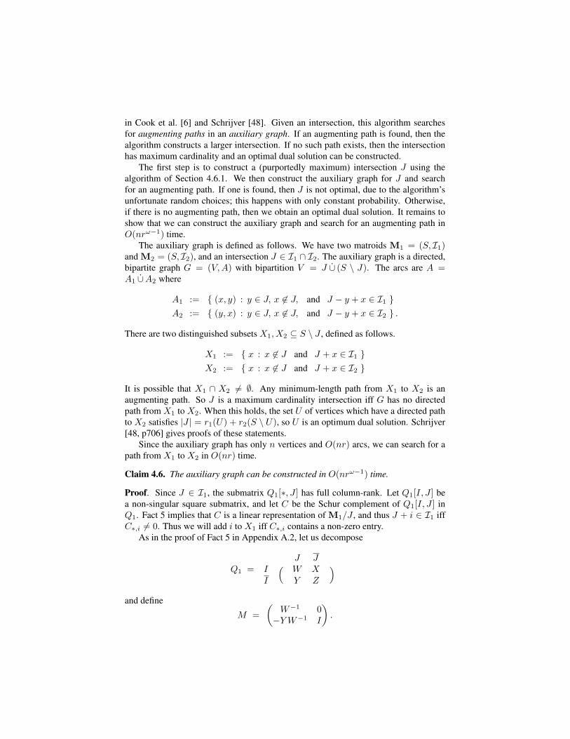
Claim 4.6. The auxiliary graph can be constructed in O(nrω−1) time.

Proof. Since J ∈ I1, the submatrix Q1[∗, J ] has full column-rank. Let Q1[I, J ] bea non-singular square submatrix, and let C be the Schur complement of Q1[I, J ] inQ1. Fact 5 implies that C is a linear representation of M1/J , and thus J + i ∈ I1 iffC∗,i 6= 0. Thus we will add i to X1 iff C∗,i contains a non-zero entry.

As in the proof of Fact 5 in Appendix A.2, let us decompose

Q1 =J J

I ( W X )I Y Z

and define

M =(

W−1 0−Y W−1 I

).

Then M ·Q1 is a linear representation of M1. Consider the decomposition

M ·Q1 =J X1 J ∪X1

I(

I W−1X∗,X1 W−1X∗,X1

)I 0 C∗,X1 0

(4.6)

Clearly Q1[∗, J − i + j] has full column-rank iff (M · Q1)[∗, J − i + j] has full-column rank. For j ∈ J ∪X1, it is clear from Eq. (4.6) that the latter condition holdsiff (M ·Q1)i,j 6= 0.

The arcs in A1 are constructed as follows. For any x ∈ X1, we have J + x ∈ I1,which implies that J + x − y ∈ I1 ∀y ∈ J . Thus (x, y) ∈ A1 for all x ∈ X1 andy ∈ J . For any x ∈ S \ (J ∪X1), we have (x, y) ∈ A1 iff (M ·Q1)i,j 6= 0, as arguedabove.

The computational cost of this procedure is dominated by the time to computeM · Q1, which clearly takes O(nrω−1) time. A symmetric argument shows how tobuild X2 and A2. ¥

5 DiscussionThis paper leaves open several questions.

• A common generalization of non-bipartite matching and matroid intersection isthe matroid matching problem [35, 37, 48]. It seems likely that our matchingand matroid intersection algorithms can be combined and extended to solve thisproblem as well, when the given matroids are linear.

• As mentioned earlier, there exist fast algorithms for rectangular matrix multipli-cation [7]. Can these be used to obtain a faster algorithm for matroid intersec-tion?

• Do Theorem 4.1 and Theorem 4.2 have other applications?

Another common generalization of non-bipartite matching and matroid intersectionis the basic path matching problem [12, 13, 11] (or independent even factor problem[11, 31]). The techniques presented herein can be extended to solve that problem, whenthe given matroids are linear. A sketch of the argument was given in a preliminaryversion of this paper [28]. For the sake of brevity, we omit further discussion of thistopic.

AcknowledgementsThe author thanks Michel Goemans, Satoru Iwata, and David Karger for helpful dis-cussions on this topic. Additionally, the author thanks the anonymous referees forsuggesting numerous improvements to the text of the paper and a concise proof ofTheorem 4.1. This work was supported by a Natural Sciences and Engineering Re-search Council of Canada PGS Scholarship, by NSF contract CCF-0515221 and byONR grant N00014-05-1-0148.

References[1] M. Aigner and T. A. Dowling. Matching theory for combinatorial geometries. Transactions of the

American Mathematical Society, 158(1):231–245, July 1971.

[2] A. I. Barvinok. New algorithms for linear k-matroid intersection and matroid k-parity problems. Math-ematical Programming, 69:449–470, 1995.

[3] P. M. Camerini, G. Galbiati, and F. Maffioli. Random pseudo-polynomial algorithms for exact matroidproblems. Journal of Algorithms, 13(2):258–273, 1992.

[4] P. Chalasani and R. Motwani. Approximating capacitated routing and delivery problems. SIAM Journalon Computing, 26(6):2133–2149, 1999.

[5] J. Cheriyan. Randomized O(M(|V |)) algorithms for problems in matching theory. SIAM Journal onComputing, 26(6):1635–1669, 1997.

[6] W. J. Cook, W. H. Cunningham, W. R. Pulleyblank, and A. Schrijver. Combinatorial Optimization.Wiley, 1997.

[7] D. Coppersmith. Rectangular matrix multiplication revisited. Journal of Complexity, 13(1):42–49,1997.

[8] D. Coppersmith and S. Winograd. Matrix multiplication via arithmetic progressions. Journal of Sym-bolic Computation, 9(3):251–280, 1990.

[9] T. H. Cormen, C. E. Leiserson, R. L. Rivest, and C. Stein. Introduction to Algorithms. MIT Press,Cambridge, MA, second edition, 2001.

[10] W. H. Cunningham. Improved bounds for matroid partition and intersection algorithms. SIAM Journalon Computing, 15(4):948–957, Nov. 1986.

[11] W. H. Cunningham and J. F. Geelen. Vertex-disjoint directed paths and even circuits. Manuscript.

[12] W. H. Cunningham and J. F. Geelen. The optimal path-matching problem. In Proceedings of the 37thAnnual IEEE Symposium on Foundations of Computer Science (FOCS), pages 78–85, 1996.

[13] W. H. Cunningham and J. F. Geelen. The optimal path-matching problem. Combinatorica, 17(3):315–337, 1997.

[14] J. Edmonds. Maximum matching and a polyhedron with 0,1-vertices. Journal of Research of theNational Bureau of Standards, 69B:125–130, 1965.

[15] J. Edmonds. Paths, trees, and flowers. Canadian Journal of Mathematics, 17:449–467, 1965.

[16] J. Edmonds. Matroid partition. In G. B. Dantzig and A. F. Veinott Jr., editors, Mathematics of theDecision Sciences Part 1, volume 11 of Lectures in Applied Mathematics, pages 335–345. AmericanMathematical Society, 1968.

[17] J. Edmonds. Submodular functions, matroids, and certain polyhedra. In R. Guy, H. Hanani, N. Sauer,and J. Schonheim, editors, Combinatorial Structures and Their Applications, pages 69–87. Gordon andBreach, 1970. Republished in M. Junger, G. Reinelt, G. Rinaldi, editors, Combinatorial Optimization– Eureka, You Shrink!, Lecture Notes in Computer Science 2570, pages 11–26. Springer-Verlag, 2003.

[18] J. Edmonds. Matroid intersection. In P. L. Hammer, E. L. Johnson, and B. H. Korte, editors, DiscreteOptimization I, volume 4 of Annals of Discrete Mathematics, pages 39–49. North-Holland, 1979.

[19] S. Even and O. Kariv. An O(n2.5) algorithm for maximum matching in general graphs. In Proceedingsof the 16th Annual IEEE Symposium on Foundations of Computer Science (FOCS), pages 100–112,1975.

[20] S. Fujishige. Submodular Functions and Optimization, volume 58 of Annals of Discrete Mathematics.Elsevier, second edition, 2005.

[21] H. N. Gabow and Y. Xu. Efficient algorithms for independent assignments on graphic and linearmatroids. In Proceedings of the 30th Annual IEEE Symposium on Foundations of Computer Science(FOCS), pages 106–111, 1989.

[22] H. N. Gabow and Y. Xu. Efficient theoretic and practical algorithms for linear matroid intersectionproblems. Journal of Computer and System Sciences, 53(1):129–147, 1996.

[23] J. F. Geelen. Matching theory. Lecture notes from the Euler Institute for Discrete Mathematics and itsApplications, 2001.

[24] C. D. Godsil. Algebraic Combinatorics. Chapman & Hall, 1993.

[25] M. X. Goemans. Bounded degree minimum spanning trees. In Proceedings of the 21st Annual IEEESymposium on Foundations of Computer Science (FOCS), 2006.

[26] A. V. Goldberg and A. V. Karzanov. Maximum skew-symmetric flows and matchings. MathematicalProgramming, 100(3):537–568, July 2004.

[27] G. H. Golub and C. F. Van Loan. Matrix Computations. Johns Hopkins University Press, third edition,1996.

[28] N. J. A. Harvey. Algebraic structures and algorithms for matching and matroid problems. In Pro-ceedings of the 47th Annual IEEE Symposium on Foundations of Computer Science (FOCS), pages531–542, 2006.

[29] N. J. A. Harvey, D. R. Karger, and K. Murota. Deterministic network coding by matrix completion.In Proceedings of the Sixteenth Annual ACM-SIAM Symposium on Discrete Algorithms (SODA 05),pages 489–498, 2005.

[30] R. Hassin and A. Levin. An efficient polynomial time approximation scheme for the constrainedminimum spanning tree problem using matroid intersection. SIAM Journal on Computing, 33(2):261–268, 2004.

[31] S. Iwata and K. Takazawa. The independent even factor problem. In Proceedings of the EighteenthAnnual ACM-SIAM Symposium on Discrete Algorithms (SODA 07), pages 1171–1180, 2007.

[32] H. J. Karloff. A Las Vegas RNC algorithm for maximum matching. Combinatorica, 6(4):387–391,1986.

[33] D. E. Knuth. The asymptotic number of geometries. Journal of Combinatorial Theory, Series A,16:398–400, 1974.

[34] E. L. Lawler. Matroid intersection algorithms. Mathematical Programming, 9:31–56, 1975.

[35] E. L. Lawler. Combinatorial Optimization: Networks and Matroids. Dover, 2001.

[36] L. Lovasz. On determinants, matchings and random algorithms. In L. Budach, editor, Fundamentalsof Computation Theory, FCT ’79, pages 565–574. Akademie-Verlag, Berlin, 1979.

[37] L. Lovasz and M. D. Plummer. Matching Theory. Akademiai Kiado – North Holland, Budapest, 1986.

[38] S. Micali and V. V. Vazirani. An O(√

V E) algorithm for finding maximum matching in generalgraphs. In Proceedings of the 21st Annual IEEE Symposium on Foundations of Computer Science(FOCS), pages 17–27, 1980.

[39] R. Motwani and P. Raghavan. Randomized Algorithms. Cambridge University Press, 1995.

[40] M. Mucha. Finding Maximum Matchings via Gaussian Elimination. PhD thesis, Warsaw University,2005.

[41] M. Mucha and P. Sankowski. Maximum matchings via Gaussian elimination. In Proceedings of the45th Annual IEEE Symposium on Foundations of Computer Science (FOCS), pages 248–255, 2004.

[42] K. Murota. Matrices and Matroids for Systems Analysis. Springer-Verlag, 2000.

[43] K. Murota. Discrete Convex Analysis. SIAM, 2003.

[44] H. Narayanan, H. Saran, and V. V. Vazirani. Randomized parallel algorithms for matroid union andintersection, with applications to arboresences and edge-disjoint spanning trees. SIAM Journal onComputing, 23(2):387–397, 1994.

[45] J. G. Oxley. Matroid Theory. Oxford University Press, 1992.

[46] M. O. Rabin and V. V. Vazirani. Maximum matchings in general graphs through randomization. Jour-nal of Algorithms, 10(4):557–567, 1989.

[47] P. Sankowski. Processor efficient parallel matching. In Proceedings of the 17th ACM Symposium onParallelism in Algorithms and Architectures (SPAA), pages 165–170, 2005.

[48] A. Schrijver. Combinatorial Optimization: Polyhedra and Efficiency. Springer-Verlag, 2003.

[49] A. Schrijver. On the history of combinatorial optimization (till 1960). In K. Aardal, G. L. Nemhauser,and R. Weismantel, editors, Discrete Optimization, volume 12 of Handbooks in Operations Researchand Management Science, pages 1–68. North Holland, 2005.

[50] N. Tomizawa and M. Iri. An algorithm for determining the rank of a triple matrix product AXB withapplication to the problem of discerning the existence of the unique solution in a network. Electronicsand Communications in Japan (Scripta Electronica Japonica II), 57(11):50–57, Nov. 1974.

[51] W. T. Tutte. The factorization of linear graphs. Journal of the London Mathematical Society, 22:107–111, 1947.

[52] V. V. Vazirani. A theory of alternating paths and blossoms for proving correctness of the O(√

V E)general graph matching algorithm. In Proceedings of the 1st Integer Programming and CombinatorialOptimization Conference (IPCO), pages 509–530, 1990.

[53] D. J. A. Welsh. Matroid Theory, volume 8 of London Mathematical Society Monographs. AcademicPress, 1976.

[54] H. Whitney. On the abstract properties of linear dependence. American Journal of Mathematics,57:509–533, 1935.

A Additional ProofsA.1 Facts from Linear Algebra

This section proves the basic facts that are given in Section 2.

Proof (of Fact 1). Note that(

I−U I

)·(

I V T

M + UV T

)=

(I V T

−U M

)=

(I V TM−1

I

)·(

I + V TM−1U−U M

).

Taking determinants shows that det(M +UV T) = det(I +V TM−1U) ·det(M). Thisproves the first claim.

The second claim follows since(M−1 −M−1U(I + V TM−1U)−1V TM−1

)·(M + UV T

)

= I + M−1U(I − (I + V TM−1U)−1 − (I + V TM−1U)−1V TM−1U

)V T

= I + M−1U(I + V TM−1U)−1((I + V TM−1U)− I − V TM−1U

)V T

= I,

as required. This proof of the second claim is well-known, and may be found in Goluband Van Loan [27, §2.1.3]. ¥

Proof (of Corollary 2.1). Let us write M = M + UV T, where

M =S S

S ( MS,S MS,S)

S MS,S MS,S

M =S S

S(

MS,S MS,S)

S MS,S MS,S

U =S

S(

I)

S 0V T =

S S

S(

MS,S−MS,S 0) .

Then Fact 1 shows that M is non-singular iff I + V TM−1U is non-singular. Using thedefinition of N , V and U , we get

I + V TNU = I + (MS,S −MS,S)NS,S .

Furthermore, Fact 1 also shows that

M−1 = N − N U (I + V TNU)−1 V T N

= N − N∗,S(I + (MS,S −MS,S)NS,S

)−1 (MS,S −MS,S)NS,∗,

as required. ¥

Proof (of Fact 2). Note that(

W −XZ−1Y 00 Z

)=

(I −XZ−1

0 I

)

︸ ︷︷ ︸N1

·(

W XY Z

)·

(I 0

−Z−1Y I

)

︸ ︷︷ ︸N2

.

(A.1)

Taking the determinant of both sides gives

det(W −XZ−1Y

) · detZ = detM,

since detN1 = det N2 = 1. This proves the first property.Furthermore, since N1 and N2 have full rank, we have

rankM = rank(W −XZ−1Y

)+ rank Z = rank C + |S2|. (A.2)

Now suppose that CA,B is non-singular with |A| = |B| = rank C. Then we have(

CA,B 00 Z

)=

(I −XA,∗Z−1

0 I

)·(

WA,B XA,∗Y∗,B Z

)·(

I 0−Z−1Y∗,B I

). (A.3)

It follows from Eq. (A.2) and Eq. (A.3) that

rankM = rank C + rank Z = rank CA,B + rank Z = rank MA∪S2,B∪S2 ,

which proves the second property. ¥

Proof (of Fact 3). Suppose that M−1 exists. Then

(M−1)i,j =((M−1)T )j,i =

((MT)−1 )j,i =

((−M)−1 )j,i = − (M−1)j,i,

as required. ¥

A.2 Proof of Fact 5

Let us write Q as

Q =B B

A(

W X)

A Y Z.

For any non-singular matrix M , the matrix M ·Q is also a linear representation of M.We choose

M =(

W−1 0−Y W−1 I

),

so that

M ·Q =(

I W−1X0 Z − Y W−1X

).

Note that C := Z−Y W−1X is the Schur complement of Q[A,B] in Q. Fact 2 showsthat C[A′, B′] is a maximum rank square submatrix of C iff Q[A ∪ A′, B ∪ B′] is amaximum rank square submatrix of Q. In other words,

{ B′ ⊆ S \ T : C[∗, B′] has full column-rank }= { B′ ⊆ S \ T : Q[∗, B ∪B′] has full column rank } ,

= { B′ ⊆ S \ T : B ∪B′ ∈ B } ,

where B is the base family of M. This family of sets is precisely BM/T , so C[∗, T ] isa linear representation of M/T . Since

C[∗, T ] = Q[A, T ]−Q[A,B] ·Q[A,B]−1 ·Q[A, T ]

the claim is proven.

A.3 Proof of Theorem 4.1

By applying elementary row and column operations (as in the proof of Fact 5 in Ap-pendix A.2), we may transform Z(J) into the form

Z(J) :=

QJ1 QJJ

1

QJ1

QJ2

QJJ2 QJ

2 T (J)J,J

,

where QJ1 has full row-rank, QJ

2 has full column-rank, QJ1 is a linear representation of

M1/J , and QJ2 is a linear representation of M2/J . Then we have

rankZ(J) = rank Z(J) = r1(J) + r2(J) + rank Z(J),

where

Z(J) :=

(QJ

1

QJ2 T (J)J,J

).

By the previously known special case of Theorem 4.1 due to Tomizawa and Iri [50],we have

rank Z(J) = |J |+ λ(J) = n− |J |+ λ(J).

Thus we haverankZ(J) = r1(J) + r2(J) + n− |J |+ λ(J),

as required.

A.4 Proof of Theorem 4.2

Claim A.1. Let J be an intersection of M1 and M2. J is extensible iff λ(∅) = λ(J)+|J |.

Proof. Suppose that J is an extensible intersection. This means that there exists anintersection I with J ⊆ I and |I| = λ(∅). Since J ∈ Ii, it is a base for itself in Mi.Thus, Eq. (4.1) shows that I \ J ∈ IMi/J for both i, implying that λ(J) ≥ |I \ J | =λ(∅)− |J |.

To show the reverse inequality, let I be a maximum cardinality intersection ofM1/J and M2/J . So |I| = λ(J). Then I ∪ J is an intersection of M1 and M2,showing that λ(∅) ≥ λ(J) + |J |. This establishes the forward direction.

Now suppose that λ(J) = λ(∅)− |J |. Then there exists an intersection I of M1/Jand M2/J with |I| = λ(∅) − |J |. Then I ∪ J is an intersection of M1 and M2, ofcardinality |I|+ |J | = λ(∅). This shows that J is contained in a maximum cardinalityintersection of M1 and M2, and therefore is extensible. ¥

Claim A.2. Assume that M1 and M2 have the same rank r. For any set J ⊆ S, wehave λ(J) ≤ r −maxi∈{1,2} ri(J).

Proof. Note that λ(J) is at most the rank of Mi/J , which is r − ri(J). ¥Suppose that J is an extensible intersection. This implies that r1(J) = |J | and

r2(J) = |J | and λ(J) = λ(∅)− |J |, by Claim A.1. Theorem 4.1 then shows that

rankZ(J) = n + r1(J) + r2(J)− |J |+ λ(J)= n + |J |+ |J | − |J |+ λ(∅)− |J |= n + r,

and hence Z(J) is non-singular as required.We now argue the converse. Clearly r2(J) ≤ |J | and, by Claim A.2, we have

λ(J) + r1(J) ≤ r. Thus

rank Z(J) = n + r1(J) + r2(J)− |J |+ λ(J)

= n +(r1(J) + λ(J)

)+

(r2(J)− |J |)

≤ n + r.

If Z(J) is non-singular then equality holds, so we have r2(J) = |J | and r1(J) +λ(J) = r. By symmetry, we also have r1(J) = |J |, implying that J is an intersection.Altogether this shows that |J |+ λ(J) = r, implying that J is extensible.