alcohol quantity and quality price elasticities: quantile...

This is a repository copy of Alcohol quantity and quality price elasticities: quantile regression estimates.

White Rose Research Online URL for this paper:http://eprints.whiterose.ac.uk/137020/

Version: Published Version

Article:

Pryce, R. orcid.org/0000-0002-4853-0719, Hollingsworth, B. and Walker, I. (2018) Alcohol quantity and quality price elasticities: quantile regression estimates. European Journal of Health Economics. ISSN 1618-7598

https://doi.org/10.1007/s10198-018-1009-8

[email protected]://eprints.whiterose.ac.uk/

Reuse

This article is distributed under the terms of the Creative Commons Attribution (CC BY) licence. This licence allows you to distribute, remix, tweak, and build upon the work, even commercially, as long as you credit the authors for the original work. More information and the full terms of the licence here: https://creativecommons.org/licenses/

Takedown

If you consider content in White Rose Research Online to be in breach of UK law, please notify us by emailing [email protected] including the URL of the record and the reason for the withdrawal request.

mailto:[email protected]

https://eprints.whiterose.ac.uk/

Vol.:(0123456789)1 3

The European Journal of Health Economics

https://doi.org/10.1007/s10198-018-1009-8

ORIGINAL PAPER

Alcohol quantity and quality price elasticities: quantile regression estimates

Robert Pryce1 · Bruce Hollingsworth2 · Ian Walker3

Received: 30 May 2018 / Accepted: 25 September 2018

© The Author(s) 2018

Abstract

Many people drink more than the recommended level of alcohol, with some drinking substantially more. There is evidence

that suggests that this leads to large health and social costs, and price is often proposed as a tool for reducing consumption.

This paper uses quantile regression methods to estimate the diferential price (and income) elasticities across the drink-

ing distribution. This is also done for on-premise (pubs, bars and clubs) and of-premise (supermarkets and shops) alcohol

separately. In addition, we examine the extent to which drinkers respond to price changes by varying the ‘quality’ of the

alcohol that they consume. We ind that heavy drinkers are much less responsive to price in terms of quantity, but that they

are more likely to substitute with cheaper products when the price of alcohol increases. The implication is that price-based

policies may have little efect in reducing consumption amongst the heaviest drinkers, provided they can switch to lower

quality alternatives.

Keywords Alcohol demand · Quantile regression · Quality elasticity

JEL Classiication D12 · I18

Introduction

UK household expenditure on alcohol in 2014 was over

£20 billion or around 4% of GNP. Over 500 million litres of

pure alcohol (equivalent to approximately 2 bottles of wine

per-adult per week) was cleared by Her Majesty’s Revenue

and Customs, generating over £9 billion in tax revenue [1].

The social cost of alcohol in the United Kingdom has been

estimated at over £21 billion, of which £3.5 billion is attrib-

uted to health costs, £11 billion to crime, and £7 billion to

lost productivity. The problem is not unique to the United

Kingdom: according to World Health Organisation, alcohol

is the second largest risk factor for disease and disability in

Europe [2]. WHO advocates tax increase as one means of

reducing consumption [2]. However, majority of the popu-

lation (69% of men, 84% of women [3]) drink within the

guidelines and any price-based policy, such as tax increase,

would have a negative efect on these people, reducing the

consumer surplus that they enjoy. Findings in the literature

suggest a nonlinear relationship between alcohol consump-

tion and overall mortality for both males and females [4].

This pattern is also found for speciic health conditions

including liver cirrhosis [5], oral and pharyngeal cancers

[6], and stroke [7]. Whether this nonlinearity constitutes a

J-curve is, however, a point of debate within the scientiic

literature (see, for example, Fillmore et al. [8] or Knott et al.

[9]). One important parameter for policy makers, who might

wish to reduce the overall consumption of alcohol, is the

price elasticity of demand. However, if there is evidence

of a nonlinear efect, then it might be possible to reduce

harmful drinking without penalising moderate drinkers too

greatly, providing the price elasticity was high for heavy

drinkers and low for moderate drinkers. If that were true

then taxation would reduce the harm on the heavy drinkers

without imposing a large loss in consumer surplus for mod-

erate users. Thus, it is particularly important to know how

the price elasticity of demand varies across the distribution

* Robert Pryce [email protected]

1 School of Health and Related Research, University of Sheield, 30 Regent Street, Sheield S1 4DA, UK

2 Division of Health Research, Lancaster University, Lancaster LA1 4YG, UK

3 Economics Department, Lancaster University, Lancaster LA1 4YG, UK

http://orcid.org/0000-0002-4853-0719

http://crossmark.crossref.org/dialog/?doi=10.1007/s10198-018-1009-8&domain=pdf

R. Pryce et al.

1 3

of drinking. While our prior is that heavy drinkers are likely

to have a more inelastic demand than moderate drinkers, to

the extent alcohol is addictive or habituating, there is little

evidence to substantiate these priors. The theory of rational

addiction [10] has been a major contribution to the literature

but suggests that, for a given level of consumption, long-run

price elasticities are lower than short-run ones. The usual

empirical implementation of the theory is based on a very

speciic parameterisation that does not explicitly allow the

slope of the demand curve to vary with consumption. How-

ever, we would expect addicts (rational, or otherwise) with

linear demand to have higher levels of consumption at any

price so implying a lower price elasticity.

One policy option to mitigate the problem of heavy drink-

ing is minimum unit pricing, which sets a price loor for

alcohol and so raises the price of low-priced alcohol. Since

heavy drinkers typically purchase cheaper per unit alcoholic

beverages (see, for example, Ludbrook et al. [11]), minimum

unit pricing disproportionately increases the price for heav-

ier drinkers than it does for light drinkers. Scotland intro-

duced minimum unit pricing on alcohol in May 2018, with

a loor price of 50 pence ($0.67; €0.57) per unit. Modelling

by Brennan et al. [12] suggests that a 45 pence (US$0.60;

€0.51) minimum unit price would afect the price of 12.5%

of the units purchased by ‘moderate’ drinkers compared to

30.5% of the units purchased by ‘harmful’ drinkers1. The

price elasticities in this modelling predict that a 45 pence

minimum unit price would decrease consumption by 0.6%

for moderate drinkers, compared to a decrease of 3.7%

for harmful drinkers. However, the modelling is based on

pseudo-panel estimates that impose a constant price elastic-

ity across the drinking distribution2 [13]. If harmful drinkers

were less price responsive than moderate drinkers, then the

efects predicted in the modelling work will be incorrect.

Since the marginal health and social harms are assumed to

be increasing with consumption, the modelling work will

thus overstate the health and social harm reduction of mini-

mum unit pricing. The contribution of this paper is that it

examines how the response to price varies across the drink-

ing distribution using quantile regression methods. Moreo-

ver, it examines, for the irst time, how quality substitution

difers in response to price across the drinking distribution.

The contribution of this paper is that we provide estimates,

using quantile regression methods for both quantity and

quality, which show that the consumption of heavy drinkers

is less responsive to price than that of moderate drinkers.

Moreover, we also ind that they are more likely to substitute

with cheaper drinks when the price of alcohol increases. The

implication, contrary to other inluential works, is that price-

based policies may have little efect in reducing consumption

amongst the heaviest drinkers, at least when it is possible for

them to switch to lower quality alternatives.

Background literature

There is a large literature on the price elasticity of demand of

alcohol. Two meta-analyses have been undertaken. Gallet [14]

includes 132 studies, and reports a median price elasticity of

demand of − 0.535, while Wagenaar et al. [15] includes many

of the same studies and reports a mean price elasticity of

− 0.44. The fact that the median is greater than the mean sug-

gests that the distribution of elasticities found in the literature

is negatively skewed. It should also be noted that the litera-

ture reviewed in the meta-analyses is varied, including studies

looking at particular age groups (for example, adolescents).

Purshouse et al. [16] use the same underlying dataset as

used in our own analysis to estimate price elasticities for

use in policy simulation analysis. They estimate separate

elasticities for moderate and harmful drinkers, and ind that

harmful drinkers are more responsive to price changes. They

also estimate cross-price elasticities between low- and high-

quality products within a beverage type, for example, low-

and high-quality beer. These cross-price elasticities are very

small, and signiicance levels are not provided. The method

used does not account for the endogenous selection issue

raised by Koenker and Hallock [17].

The seminal work on quantile regression in the context of

alcohol demand was done by Manning et al. [18] which esti-

mates the price elasticity of demand for alcohol in the United

States. However, it uses only a single cross-section of data and

a price index (ACCRA) which is the weighted average of three

drinks (one beer, one whisky, and one wine). The variation in

price comes only from across the cross-section and so is entirely

driven by diferences in the geographical location of consum-

ers—so it is not possible to separately identify price efects

from geographical efects. While, the identiication strategy

casts serious doubt on the interpretation of the estimated price

elasticities, the results suggest a U-shaped relationship between

conditional consumption decile and price elasticity, with the

middle of the drinking distribution being most responsive to

price changes relative to the tails of the distribution. Impor-

tantly for policy, they also ind that the elasticity estimate for

the top conditional decile, where the very heaviest drinkers get

most weight, is not signiicantly diferent from zero.

1 Moderate drinkers in this context are males (females) who drink more than 21 (14) units per week. Harmful drinkers are males (females) who drink more than 50 (35) units per week. A unit is equal to 10 ml or 8 g of pure alcohol.2 Moreover, since this estimate comes from diferencing across the pseudo-lifecycles of cohorts of individuals the interpretation that should be given to the resulting elasticity is that it is the response to anticipated variation in prices across the lifecycle. The policy elastic-ity of interest here is the conventional Marshallian one that tells us the response to unanticipated changes in price.


1 3

Safer et al. [19] use the National Longitudinal Study of

Youth (NLSY) cohort study to estimate the response to price

(and advertising) changes across the drinking distribution. The

data are only concerned with those aged 18–29, so the results

may not be generalisable to the whole population. The ACCRA

price data is used. The authors use conditional quantile regres-

sion, and ind no statistically signiicant relationship between

price and consumption at any quantile and there was no statisti-

cal diference between estimates for any pair of deciles.

Byrnes et al. [20] used 3 years of Australian household

cross-section survey data, and a double-hurdle quantile regres-

sion technique, to estimate the price elasticity of demand for

alcohol. In contrast to Manning et al., the authors ind that

heavy drinkers are more responsive to price compared to

lighter drinkers, and it is the lightest drinkers whose demand

is perfectly inelastic. They also ind a relatively high average

price elasticity, close to − 1, which is much higher than the

estimates found in the meta-analyses. The authors suggest that

this inding could be speciic to Australia and not generalis-

able to other countries. The authors also discuss the possibil-

ity of switching to cheaper alcohol products to mitigate price

increase, but no analysis is carried out to test this possibility.

Gruenewald et al. [21] use time-series Swedish alcohol

retail data from 1984 to 1994 to examine the impact of a

change in the alcohol duty rates on alcohol quantity and

quality demand. In 1992, the Swedish alcohol regulator, Sys-

tembolaget, changed the structure of duties such that bever-

ages were taxed based on alcoholic strength rather than as

a percentage of pre-tax price. The duty change led to a nar-

rower distribution of prices for wine and spirits, but a wider

distribution of prices for beer. The authors deine quality by

the relative price of the drink, and assign drinks into three

categories—high, medium and low quality. This is done for

three drink types—beer, wine and spirits—giving nine dif-

ferent types. However, the study uses only time-series data,

with the dependent variable being monthly sales by drink

type, giving 120 observations for each type. The price vari-

able is a price index constructed from the unweighted aver-

age price for each of the nine drink types.

Data

The data used in this paper come from 13 years of nationally

representative, cross-sectional surveys: the UK Expenditure

and Food Survey (EFS) 2001–2007, and its successor, the

Living Costs and Food Survey 2008–2013. The surveys

are a combination of a household interview and a 2-week

expenditure diary. Detailed information on expenditure is

recorded on alcoholic drinks, including information about

the quantity (in millilitres) of alcoholic drinks purchased.

Alcohol is recorded for 25 disaggregated premise type/

drink type combinations—for example, on-trade/fortiied

wine. The consumption of drinks by type were converted

into units of ethanol using the alcohol strengths reported in

Purshouse et al. [16]. The diaries are recorded by individual

expenditures within the household but we have no informa-

tion on individual consumption, so this paper aggregates

individual expenditures to the household level because of

concerns regarding intra-household transfers.

We adopt a double log speciication for demand and only

households who purchased alcohol (68.4% of all households)

are included in the study. The reason for zero expenditure is

not known3 in our data and, in any event, it is not possible to

use a simple Tobit speciication when the dependent variable

is in log form. The presumption in our double log speciica-

tion is that there is no price that would turn a drinker into

a non-drinker (and vice versa) and so non-drinkers simply

have diferent preferences to drinkers.

We identify our price elasticities from cross-region and

cross-time (in months) variation in prices that are derived

from our microdata collapsed into region × time cells. Since

our dataset is the same dataset that is used to construct the

sub-indices of the retail prices index from observed expendi-

ture and quantities, this is a natural way of deining prices.

However, we do not include the lead and lag of consump-

tion since our data is just pooled cross-sections. Implicitly,

our speciication could be reconciled with the conventional

rational addiction speciication by treating the omitted leads

and lags as unobservables, and it deals with the efect of the

resulting heteroskedasticity on standard errors by estimating

the used robust methods.

Our survey data contains information on expenditure and

quantity—so a “unit value” can be calculated by dividing

expenditure by quantity. However, using unit values as the

price would yield biased elasticity estimates since much of

the variation in unit values would be due to variation in the

‘quality’ of alcohol consumed. That is, a diference in unit

values across households would arise because of both dif-

ferences in the true price and of diferences in (endogenous)

quality selection. If heavier drinkers have a taste for cheaper,

lower ‘quality’ alcohol, then price elasticity estimates will

be biased away from zero (i.e., will be more elastic).

For this reason, this study uses the month–region average

price-per-unit of alcohol. Thus, our measure of price captures

diferential changes over time and across region. To create

the index for a region, a mean price-per-unit is calculated

for each household in that region by summing up alcohol

expenditure and dividing by the total number of alcoholic

units. The average of these is taken for cells deined by the

12 regions in the United Kingdom, and for each of the 153

3 Censored quantile regression, which assumes all zero expenditures arise due to price/income reasons in a similar manner to the Tobit model, produce broadly similar results.

R. Pryce et al.

1 3

months in the survey period.4 Note that since we include

region ixed efects and month ixed efects, our “price” vari-

able is deined as the regional × time average, and this deini-

tion is immune from the usual endogeneity arguments. We

assume that prices change in response to changes in produc-

tion costs, as well as tax changes over time.

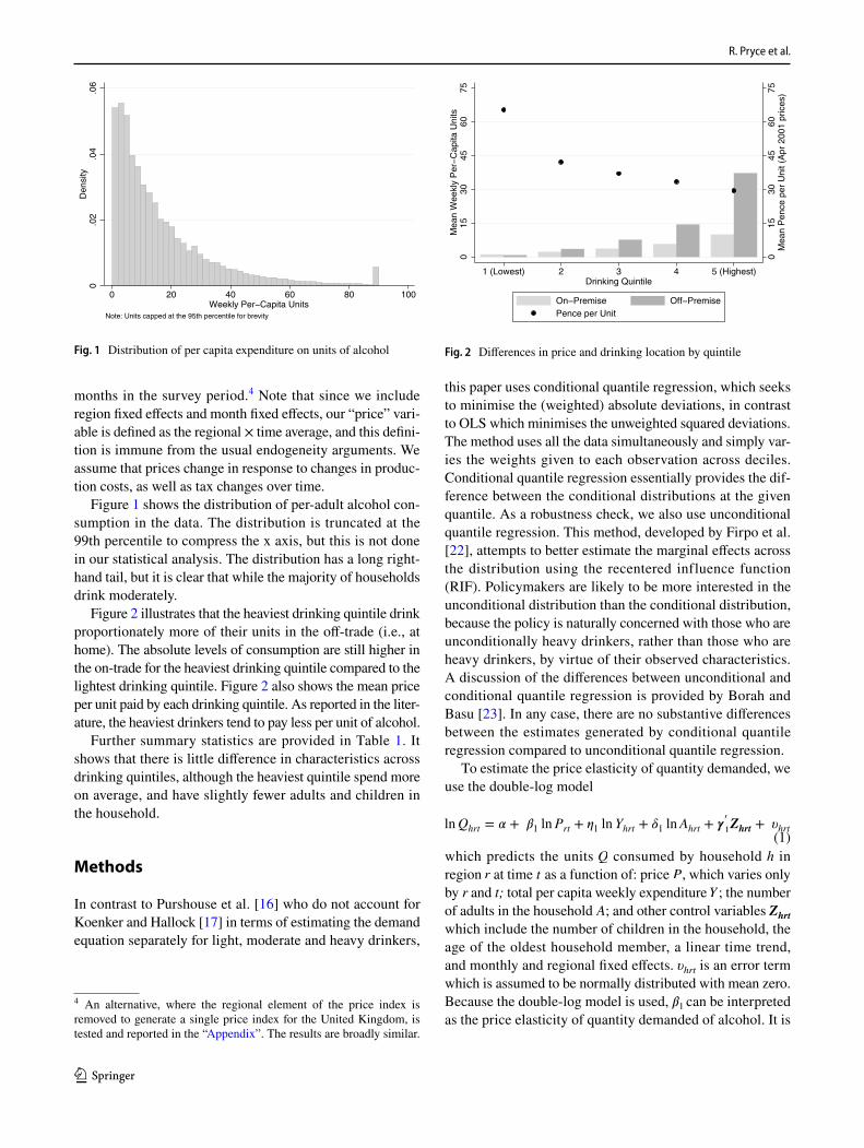
Figure 1 shows the distribution of per-adult alcohol con-

sumption in the data. The distribution is truncated at the

99th percentile to compress the x axis, but this is not done

in our statistical analysis. The distribution has a long right-

hand tail, but it is clear that while the majority of households

drink moderately.

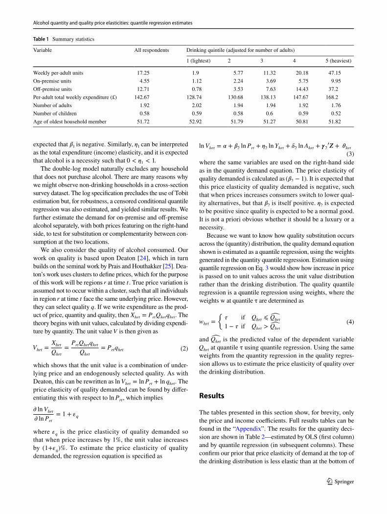
Figure 2 illustrates that the heaviest drinking quintile drink

proportionately more of their units in the of-trade (i.e., at

home). The absolute levels of consumption are still higher in

the on-trade for the heaviest drinking quintile compared to the

lightest drinking quintile. Figure 2 also shows the mean price

per unit paid by each drinking quintile. As reported in the liter-

ature, the heaviest drinkers tend to pay less per unit of alcohol.

Further summary statistics are provided in Table 1. It

shows that there is little diference in characteristics across

drinking quintiles, although the heaviest quintile spend more

on average, and have slightly fewer adults and children in

the household.

Methods

In contrast to Purshouse et al. [16] who do not account for

Koenker and Hallock [17] in terms of estimating the demand

equation separately for light, moderate and heavy drinkers,

this paper uses conditional quantile regression, which seeks

to minimise the (weighted) absolute deviations, in contrast

to OLS which minimises the unweighted squared deviations.

The method uses all the data simultaneously and simply var-

ies the weights given to each observation across deciles.

Conditional quantile regression essentially provides the dif-

ference between the conditional distributions at the given

quantile. As a robustness check, we also use unconditional

quantile regression. This method, developed by Firpo et al.

[22], attempts to better estimate the marginal efects across

the distribution using the recentered influence function

(RIF). Policymakers are likely to be more interested in the

unconditional distribution than the conditional distribution,

because the policy is naturally concerned with those who are

unconditionally heavy drinkers, rather than those who are

heavy drinkers, by virtue of their observed characteristics.

A discussion of the diferences between unconditional and

conditional quantile regression is provided by Borah and

Basu [23]. In any case, there are no substantive diferences

between the estimates generated by conditional quantile

regression compared to unconditional quantile regression.

To estimate the price elasticity of quantity demanded, we

use the double-log model

which predicts the units Q consumed by household h in

region r at time t as a function of: price P , which varies only

by r and t; total per capita weekly expenditure Y ; the number

of adults in the household A ; and other control variables Zhrt

which include the number of children in the household, the

age of the oldest household member, a linear time trend,

and monthly and regional ixed efects. �hrt

is an error term

which is assumed to be normally distributed with mean zero.

Because the double-log model is used, �1 can be interpreted

as the price elasticity of quantity demanded of alcohol. It is

(1)ln Qhrt = � + �

1ln Prt + �

1ln Yhrt + �

1ln Ahrt + �

�

1Z

hrt+ �hrt

0.0

2.0

4.0

6D

ensity

0 20 40 60 80 100Weekly Per−Capita Units

Note: Units capped at the 95th percentile for brevity

Fig. 1 Distribution of per capita expenditure on units of alcohol

01

53

04

56

07

5M

ea

n P

en

ce

pe

r U

nit (

Ap

r 2

00

1 p

rice

s)

01

53

04

56

07

5M

ea

n W

ee

kly

Pe

r−C

ap

ita

Un

its

1 (Lowest) 5 (Highest)2 3 4Drinking Quintile

On−Premise Off−Premise

Pence per Unit

Fig. 2 Diferences in price and drinking location by quintile

4 An alternative, where the regional element of the price index is removed to generate a single price index for the United Kingdom, is tested and reported in the “Appendix”. The results are broadly similar.


1 3

expected that �1 is negative. Similarly, �

1 can be interpreted

as the total expenditure (income) elasticity, and it is expected

that alcohol is a necessity such that 0 < �1< 1.

The double-log model naturally excludes any household

that does not purchase alcohol. There are many reasons why

we might observe non-drinking households in a cross-section

survey dataset. The log speciication precludes the use of Tobit

estimation but, for robustness, a censored conditional quantile

regression was also estimated, and yielded similar results. We

further estimate the demand for on-premise and of-premise

alcohol separately, with both prices featuring on the right-hand

side, to test for substitution or complementarity between con-

sumption at the two locations.

We also consider the quality of alcohol consumed. Our

work on quality is based upon Deaton [24], which in turn

builds on the seminal work by Prais and Houthakker [25]. Dea-

ton’s work uses clusters to deine prices, which for the purpose

of this work will be regions r at time t . True price variation is

assumed not to occur within a cluster, such that all individuals

in region r at time t face the same underlying price. However,

they can select quality q . If we write expenditure as the prod-

uct of price, quantity and quality, then Xhrt = PrtQhrtqhrt . The

theory begins with unit values, calculated by dividing expendi-

ture by quantity. The unit value V is then given as

which shows that the unit value is a combination of under-

lying price and an endogenously selected quality. As with

Deaton, this can be rewritten as ln Vhrt = ln Prt + ln qhrt . The

price elasticity of quality demanded can be found by difer-

entiating this with respect to ln Prt , which implies

where �q is the price elasticity of quality demanded so

that when price increases by 1%, the unit value increases

by (1+�q)%. To estimate the price elasticity of quality

demanded, the regression equation is speciied as

(2)Vhrt =Xhrt

Qhrt

=

PrtQhrtqhrt

Qhrt

= Prtqhrt

� ln Vhrt

� ln Prt

= 1 + �q

where the same variables are used on the right-hand side

as in the quantity demand equation. The price elasticity of

quality demanded is calculated as (�2− 1) . It is expected that

this price elasticity of quality demanded is negative, such

that when prices increases consumers switch to lower qual-

ity alternatives, but that �2 is itself positive. �

2 is expected

to be positive since quality is expected to be a normal good.

It is not a priori obvious whether it should be a luxury or a

necessity.

Because we want to know how quality substitution occurs

across the (quantity) distribution, the quality demand equation

shown is estimated as a quantile regression, using the weights

generated in the quantity quantile regression. Estimation using

quantile regression on Eq. 3 would show how increase in price

is passed on to unit values across the unit value distribution

rather than the drinking distribution. The quality quantile

regression is a quantile regression using weights, where the

weights w at quantile τ are determined as

and Q̂hrt is the predicted value of the dependent variable

Qhrt at quantile τ using quantile regression. Using the same

weights from the quantity regression in the quality regres-

sion allows us to estimate the price elasticity of quality over

the drinking distribution.

Results

The tables presented in this section show, for brevity, only

the price and income coeicients. Full results tables can be

found in the “Appendix”. The results for the quantity deci-

sion are shown in Table 2—estimated by OLS (irst column)

and by quantile regression (in subsequent columns). These

conirm our prior that price elasticity of demand at the top of

the drinking distribution is less elastic than at the bottom of

(3)

ln Vhrt

= � + �2

ln Prt+ �

2ln Y

hrt+ �

2ln A

hrt+ �

2

�Z + �

hrt

(4)whrt =

{

� if Qhrt ⩽�Qhrt

1 − � if Qhrt >�Qhrt

Table 1 Summary statistics

Variable All respondents Drinking quintile (adjusted for number of adults)

1 (lightest) 2 3 4 5 (heaviest)

Weekly per-adult units 17.25 1.9 5.77 11.32 20.18 47.15

On-premise units 4.55 1.12 2.24 3.69 5.75 9.95

Of-premise units 12.71 0.78 3.53 7.63 14.43 37.2

Per-adult total weekly expenditure (£) 142.67 128.74 130.68 138.13 147.67 168.2

Number of adults 1.92 2.02 1.94 1.94 1.92 1.76

Number of children 0.58 0.59 0.58 0.6 0.59 0.52

Age of oldest household member 51.72 52.92 51.79 51.27 50.81 51.82

R. Pryce et al.

1 3

the distribution: the lower quartile’s price elasticity is − 0.709

compared to − 0.346 for the upper quartile. Unlike some ind-

ings in the literature, we ind that no part of the drinking

distribution is perfectly price inelastic. The income (total

expenditure per capita) elasticity is positive, but less than

1, so that alcohol is a normal good. The efect of income is

fairly constant across the drinking distribution. The positive

coeicient on the log number of adults in the “Appendix”

shows that for every extra adult in the household, household

consumption increases but at a decreasing rate. The monthly

ixed efects show that consumption increases signiicantly

in November and December, whilst the North East and North

West drink signiicantly more than any other region.

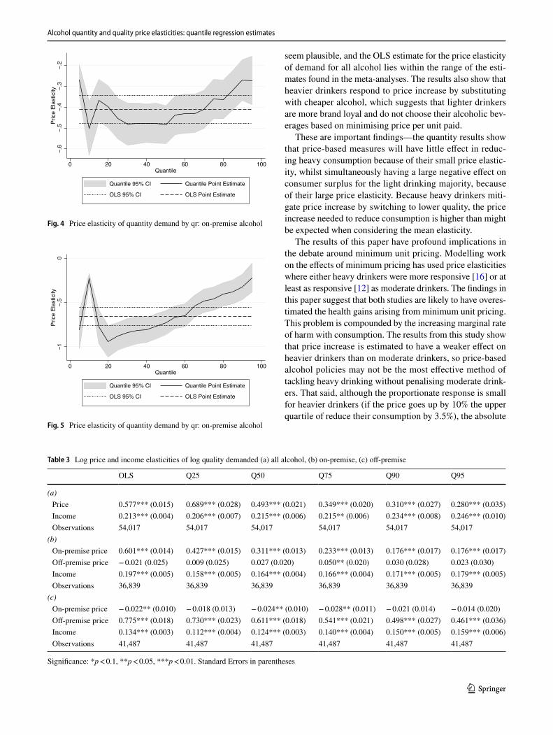
The results for on- and of-premise alcohol are presented

in Table 2b and c, respectively. They suggest that there is

zero cross-price elasticity of demand. The demand for of-

premise alcohol is more price elastic than the demand for

on-premise alcohol. Perhaps surprisingly, the income elas-

ticity is lower for on-premise alcohol. The detailed results

in the “Appendix” show that seasonal efect is stronger in

of-premise alcohol, with alcohol consumption increasing by

30% in December compared to January. As might perhaps

be expected, households with more children consume less

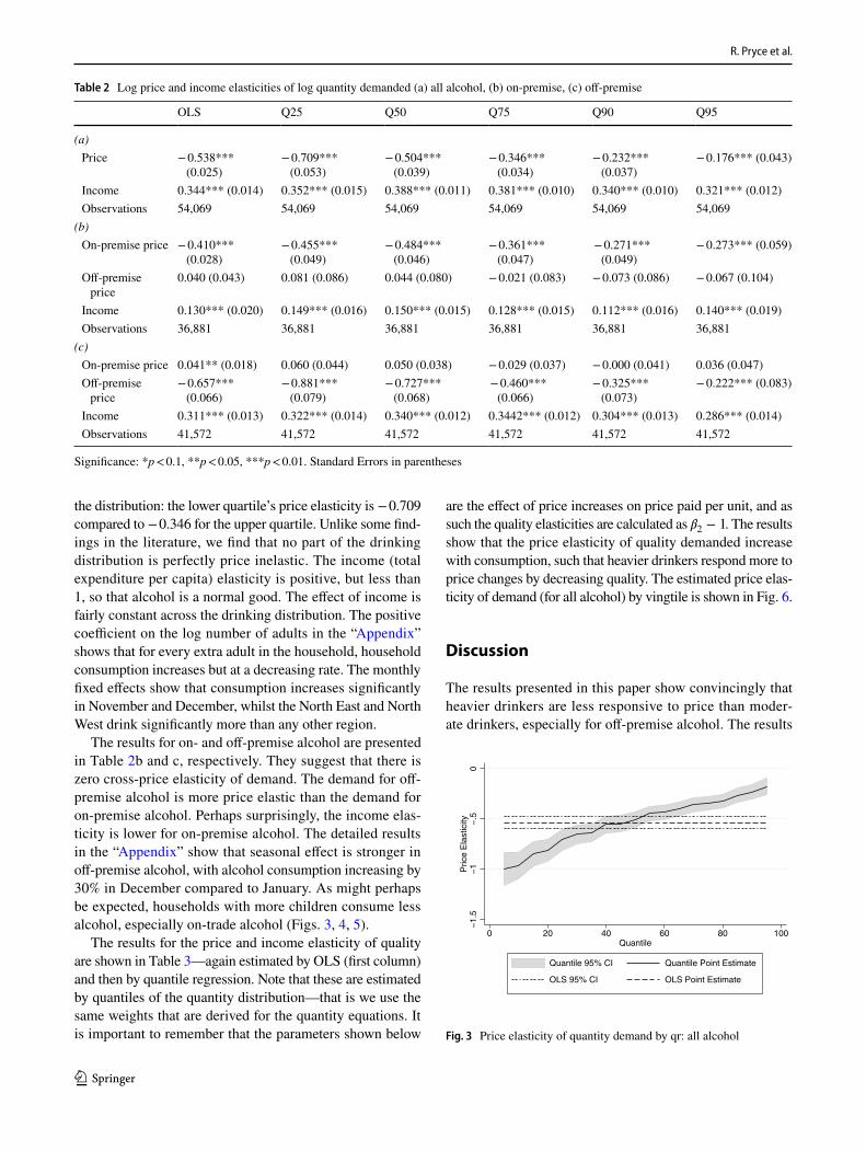
alcohol, especially on-trade alcohol (Figs. 3, 4, 5).

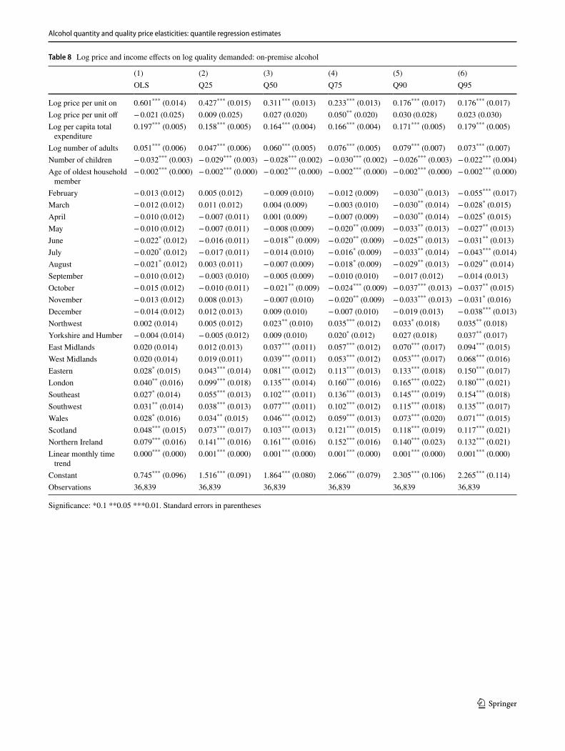
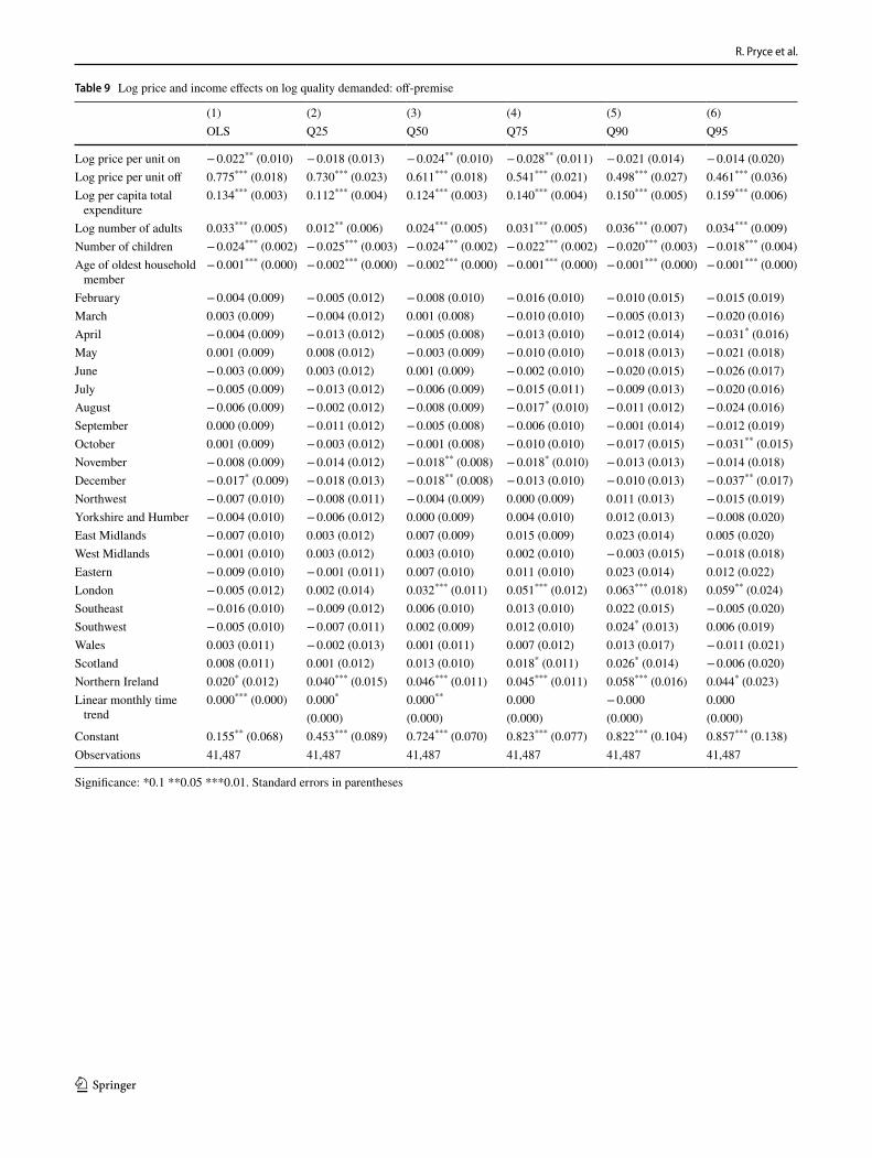
The results for the price and income elasticity of quality

are shown in Table 3—again estimated by OLS (irst column)

and then by quantile regression. Note that these are estimated

by quantiles of the quantity distribution—that is we use the

same weights that are derived for the quantity equations. It

is important to remember that the parameters shown below

are the efect of price increases on price paid per unit, and as

such the quality elasticities are calculated as �2− 1 . The results

show that the price elasticity of quality demanded increase

with consumption, such that heavier drinkers respond more to

price changes by decreasing quality. The estimated price elas-

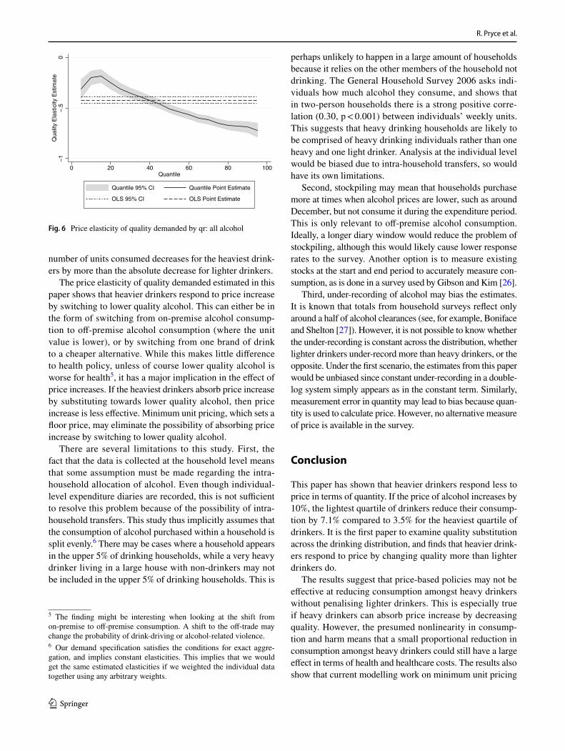
ticity of demand (for all alcohol) by vingtile is shown in Fig. 6.

Discussion

The results presented in this paper show convincingly that

heavier drinkers are less responsive to price than moder-

ate drinkers, especially for of-premise alcohol. The results

Table 2 Log price and income elasticities of log quantity demanded (a) all alcohol, (b) on-premise, (c) of-premise

Signiicance: *p < 0.1, **p < 0.05, ***p < 0.01. Standard Errors in parentheses

OLS Q25 Q50 Q75 Q90 Q95

(a)

Price − 0.538*** (0.025)

− 0.709*** (0.053)

− 0.504*** (0.039)

− 0.346*** (0.034)

− 0.232*** (0.037)

− 0.176*** (0.043)

Income 0.344*** (0.014) 0.352*** (0.015) 0.388*** (0.011) 0.381*** (0.010) 0.340*** (0.010) 0.321*** (0.012)

Observations 54,069 54,069 54,069 54,069 54,069 54,069

(b)

On-premise price − 0.410*** (0.028)

− 0.455*** (0.049)

− 0.484*** (0.046)

− 0.361*** (0.047)

− 0.271*** (0.049)

− 0.273*** (0.059)

Of-premise price

0.040 (0.043) 0.081 (0.086) 0.044 (0.080) − 0.021 (0.083) − 0.073 (0.086) − 0.067 (0.104)

Income 0.130*** (0.020) 0.149*** (0.016) 0.150*** (0.015) 0.128*** (0.015) 0.112*** (0.016) 0.140*** (0.019)

Observations 36,881 36,881 36,881 36,881 36,881 36,881

(c)

On-premise price 0.041** (0.018) 0.060 (0.044) 0.050 (0.038) − 0.029 (0.037) − 0.000 (0.041) 0.036 (0.047)

Of-premise price

− 0.657*** (0.066)

− 0.881*** (0.079)

− 0.727*** (0.068)

− 0.460*** (0.066)

− 0.325*** (0.073)

− 0.222*** (0.083)

Income 0.311*** (0.013) 0.322*** (0.014) 0.340*** (0.012) 0.3442*** (0.012) 0.304*** (0.013) 0.286*** (0.014)

Observations 41,572 41,572 41,572 41,572 41,572 41,572

−1

.5−

1−

.50

Price

Ela

sticity

0 20 40 60 80 100Quantile

Quantile 95% CI Quantile Point Estimate

OLS 95% CI OLS Point Estimate

Fig. 3 Price elasticity of quantity demand by qr: all alcohol


1 3

seem plausible, and the OLS estimate for the price elasticity

of demand for all alcohol lies within the range of the esti-

mates found in the meta-analyses. The results also show that

heavier drinkers respond to price increase by substituting

with cheaper alcohol, which suggests that lighter drinkers

are more brand loyal and do not choose their alcoholic bev-

erages based on minimising price per unit paid.

These are important indings—the quantity results show

that price-based measures will have little efect in reduc-

ing heavy consumption because of their small price elastic-

ity, whilst simultaneously having a large negative efect on

consumer surplus for the light drinking majority, because

of their large price elasticity. Because heavy drinkers miti-

gate price increase by switching to lower quality, the price

increase needed to reduce consumption is higher than might

be expected when considering the mean elasticity.

The results of this paper have profound implications in

the debate around minimum unit pricing. Modelling work

on the efects of minimum pricing has used price elasticities

where either heavy drinkers were more responsive [16] or at

least as responsive [12] as moderate drinkers. The indings in

this paper suggest that both studies are likely to have overes-

timated the health gains arising from minimum unit pricing.

This problem is compounded by the increasing marginal rate

of harm with consumption. The results from this study show

that price increase is estimated to have a weaker efect on

heavier drinkers than on moderate drinkers, so price-based

alcohol policies may not be the most efective method of

tackling heavy drinking without penalising moderate drink-

ers. That said, although the proportionate response is small

for heavier drinkers (if the price goes up by 10% the upper

quartile of reduce their consumption by 3.5%), the absolute

−.6

−.5

−.4

−.3

−.2

Price E

lasticity

0 20 40 60 80 100Quantile



Fig. 4 Price elasticity of quantity demand by qr: on-premise alcohol

−1

−.5

0P

rice E

lasticity

0 20 40 60 80 100Quantile



Fig. 5 Price elasticity of quantity demand by qr: on-premise alcohol

Table 3 Log price and income elasticities of log quality demanded (a) all alcohol, (b) on-premise, (c) of-premise

Signiicance: *p < 0.1, **p < 0.05, ***p < 0.01. Standard Errors in parentheses

OLS Q25 Q50 Q75 Q90 Q95

(a)

Price 0.577*** (0.015) 0.689*** (0.028) 0.493*** (0.021) 0.349*** (0.020) 0.310*** (0.027) 0.280*** (0.035)

Income 0.213*** (0.004) 0.206*** (0.007) 0.215*** (0.006) 0.215** (0.006) 0.234*** (0.008) 0.246*** (0.010)

Observations 54,017 54,017 54,017 54,017 54,017 54,017

(b)

On-premise price 0.601*** (0.014) 0.427*** (0.015) 0.311*** (0.013) 0.233*** (0.013) 0.176*** (0.017) 0.176*** (0.017)

Of-premise price − 0.021 (0.025) 0.009 (0.025) 0.027 (0.020) 0.050** (0.020) 0.030 (0.028) 0.023 (0.030)

Income 0.197*** (0.005) 0.158*** (0.005) 0.164*** (0.004) 0.166*** (0.004) 0.171*** (0.005) 0.179*** (0.005)

Observations 36,839 36,839 36,839 36,839 36,839 36,839

(c)

On-premise price − 0.022** (0.010) − 0.018 (0.013) − 0.024** (0.010) − 0.028** (0.011) − 0.021 (0.014) − 0.014 (0.020)

Of-premise price 0.775*** (0.018) 0.730*** (0.023) 0.611*** (0.018) 0.541*** (0.021) 0.498*** (0.027) 0.461*** (0.036)

Income 0.134*** (0.003) 0.112*** (0.004) 0.124*** (0.003) 0.140*** (0.004) 0.150*** (0.005) 0.159*** (0.006)

Observations 41,487 41,487 41,487 41,487 41,487 41,487

R. Pryce et al.

1 3

number of units consumed decreases for the heaviest drink-

ers by more than the absolute decrease for lighter drinkers.

The price elasticity of quality demanded estimated in this

paper shows that heavier drinkers respond to price increase

by switching to lower quality alcohol. This can either be in

the form of switching from on-premise alcohol consump-

tion to of-premise alcohol consumption (where the unit

value is lower), or by switching from one brand of drink

to a cheaper alternative. While this makes little diference

to health policy, unless of course lower quality alcohol is

worse for health5, it has a major implication in the efect of

price increases. If the heaviest drinkers absorb price increase

by substituting towards lower quality alcohol, then price

increase is less efective. Minimum unit pricing, which sets a

loor price, may eliminate the possibility of absorbing price

increase by switching to lower quality alcohol.

There are several limitations to this study. First, the

fact that the data is collected at the household level means

that some assumption must be made regarding the intra-

household allocation of alcohol. Even though individual-

level expenditure diaries are recorded, this is not suicient

to resolve this problem because of the possibility of intra-

household transfers. This study thus implicitly assumes that

the consumption of alcohol purchased within a household is

split evenly.6 There may be cases where a household appears

in the upper 5% of drinking households, while a very heavy

drinker living in a large house with non-drinkers may not

be included in the upper 5% of drinking households. This is

perhaps unlikely to happen in a large amount of households

because it relies on the other members of the household not

drinking. The General Household Survey 2006 asks indi-

viduals how much alcohol they consume, and shows that

in two-person households there is a strong positive corre-

lation (0.30, p < 0.001) between individuals’ weekly units.

This suggests that heavy drinking households are likely to

be comprised of heavy drinking individuals rather than one

heavy and one light drinker. Analysis at the individual level

would be biased due to intra-household transfers, so would

have its own limitations.

Second, stockpiling may mean that households purchase

more at times when alcohol prices are lower, such as around

December, but not consume it during the expenditure period.

This is only relevant to of-premise alcohol consumption.

Ideally, a longer diary window would reduce the problem of

stockpiling, although this would likely cause lower response

rates to the survey. Another option is to measure existing

stocks at the start and end period to accurately measure con-

sumption, as is done in a survey used by Gibson and Kim [26].

Third, under-recording of alcohol may bias the estimates.

It is known that totals from household surveys relect only

around a half of alcohol clearances (see, for example, Boniface

and Shelton [27]). However, it is not possible to know whether

the under-recording is constant across the distribution, whether

lighter drinkers under-record more than heavy drinkers, or the

opposite. Under the irst scenario, the estimates from this paper

would be unbiased since constant under-recording in a double-

log system simply appears as in the constant term. Similarly,

measurement error in quantity may lead to bias because quan-

tity is used to calculate price. However, no alternative measure

of price is available in the survey.

Conclusion

This paper has shown that heavier drinkers respond less to

price in terms of quantity. If the price of alcohol increases by

10%, the lightest quartile of drinkers reduce their consump-

tion by 7.1% compared to 3.5% for the heaviest quartile of

drinkers. It is the irst paper to examine quality substitution

across the drinking distribution, and inds that heavier drink-

ers respond to price by changing quality more than lighter

drinkers do.

The results suggest that price-based policies may not be

efective at reducing consumption amongst heavy drinkers

without penalising lighter drinkers. This is especially true

if heavy drinkers can absorb price increase by decreasing

quality. However, the presumed nonlinearity in consump-

tion and harm means that a small proportional reduction in

consumption amongst heavy drinkers could still have a large

efect in terms of health and healthcare costs. The results also

show that current modelling work on minimum unit pricing

−1

−.5

0Q

ualit

y E

lasticity E

stim

ate

0 20 40 60 80 100Quantile



Fig. 6 Price elasticity of quality demanded by qr: all alcohol

5 The inding might be interesting when looking at the shift from on-premise to of-premise consumption. A shift to the of-trade may change the probability of drink-driving or alcohol-related violence.6 Our demand speciication satisies the conditions for exact aggre-gation, and implies constant elasticities. This implies that we would get the same estimated elasticities if we weighted the individual data together using any arbitrary weights.


1 3

probably overstates the efects by not allowing the price elas-

ticity to vary across the drinking distribution. This means that

it predicts less consumer surplus loss for moderate drinkers,

and a greater reduction in consumption in heavy drinkers,

than would be expected given the results of this paper.

Acknowledgements We are grateful for funding from the Economic and Social Research Council. The data is provided by the UK Data Service, who are not responsible for the data analysis and indings. The data can be shared with other researchers subject to the permis-sion of the Data Service and our code is available from the corre-sponding author. This work has been granted Lancaster University ethics approval. We are grateful to three anonymous referees for their comments.

Open Access This article is distributed under the terms of the Crea-tive Commons Attribution 4.0 International License (http://creat iveco mmons .org/licen ses/by/4.0/), which permits unrestricted use, distribu-tion, and reproduction in any medium, provided you give appropriate credit to the original author(s) and the source, provide a link to the Creative Commons license, and indicate if changes were made.

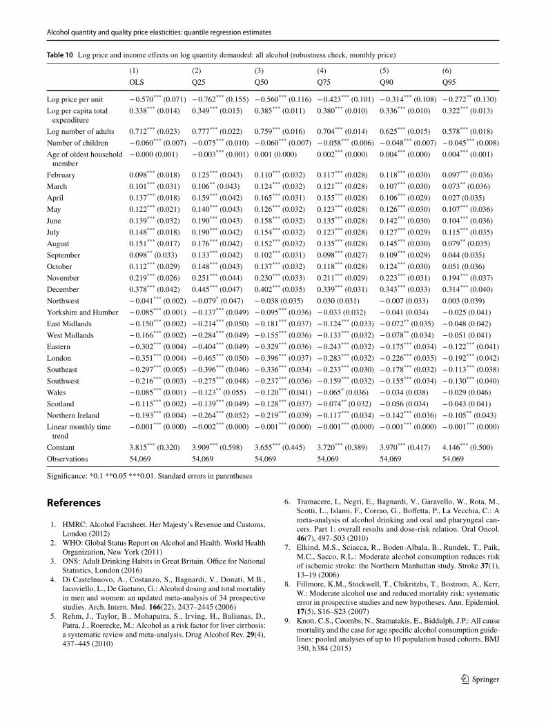
Appendix

Full regression tables are found in Tables 4, 5, 6, 7, 8, 9.

Table 10 shows the regression results using a monthly price

index (with no regional variation).

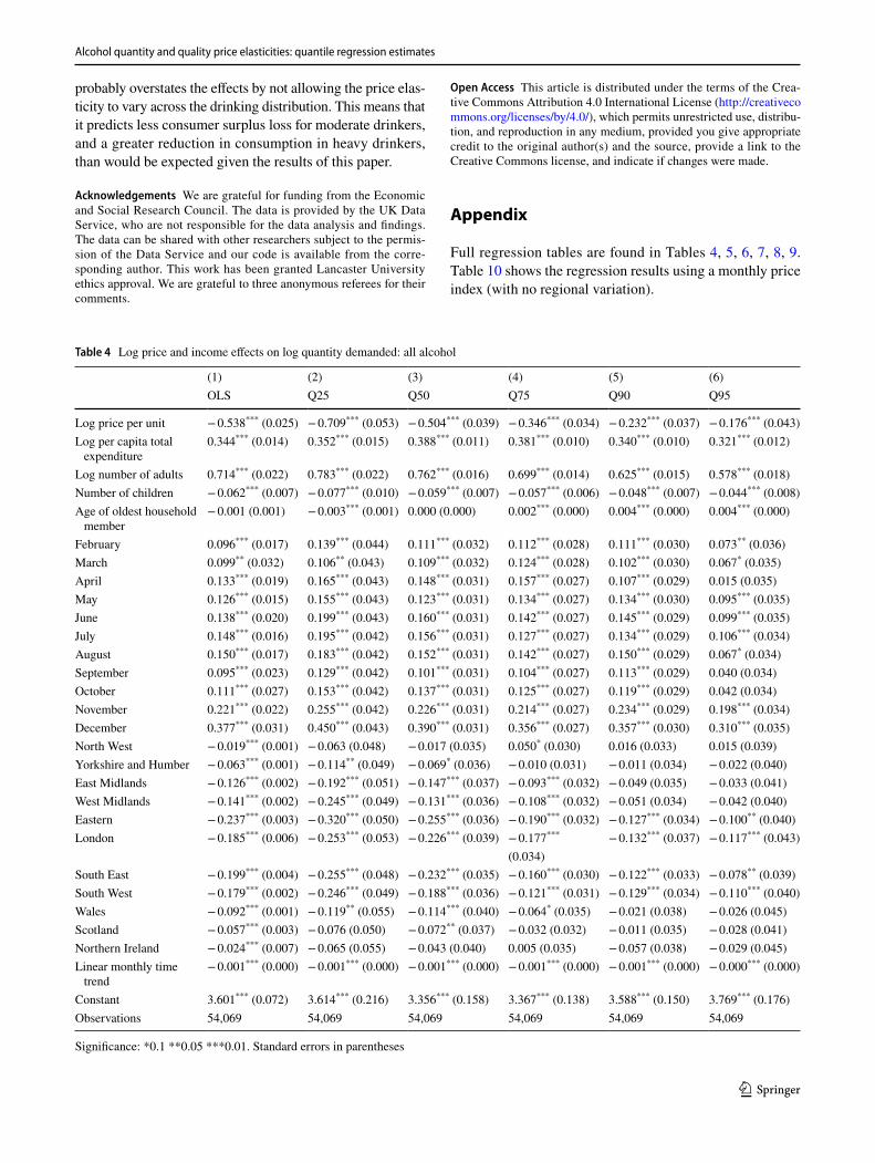
Table 4 Log price and income efects on log quantity demanded: all alcohol

Signiicance: *0.1 **0.05 ***0.01. Standard errors in parentheses

(1) (2) (3) (4) (5) (6)

OLS Q25 Q50 Q75 Q90 Q95

Log price per unit − 0.538*** (0.025) − 0.709*** (0.053) − 0.504*** (0.039) − 0.346*** (0.034) − 0.232*** (0.037) − 0.176*** (0.043)

Log per capita total expenditure

0.344*** (0.014) 0.352*** (0.015) 0.388*** (0.011) 0.381*** (0.010) 0.340*** (0.010) 0.321*** (0.012)

Log number of adults 0.714*** (0.022) 0.783*** (0.022) 0.762*** (0.016) 0.699*** (0.014) 0.625*** (0.015) 0.578*** (0.018)

Number of children − 0.062*** (0.007) − 0.077*** (0.010) − 0.059*** (0.007) − 0.057*** (0.006) − 0.048*** (0.007) − 0.044*** (0.008)

Age of oldest household member

− 0.001 (0.001) − 0.003*** (0.001) 0.000 (0.000) 0.002*** (0.000) 0.004*** (0.000) 0.004*** (0.000)

February 0.096*** (0.017) 0.139*** (0.044) 0.111*** (0.032) 0.112*** (0.028) 0.111*** (0.030) 0.073** (0.036)

March 0.099** (0.032) 0.106** (0.043) 0.109*** (0.032) 0.124*** (0.028) 0.102*** (0.030) 0.067* (0.035)

April 0.133*** (0.019) 0.165*** (0.043) 0.148*** (0.031) 0.157*** (0.027) 0.107*** (0.029) 0.015 (0.035)

May 0.126*** (0.015) 0.155*** (0.043) 0.123*** (0.031) 0.134*** (0.027) 0.134*** (0.030) 0.095*** (0.035)

June 0.138*** (0.020) 0.199*** (0.043) 0.160*** (0.031) 0.142*** (0.027) 0.145*** (0.029) 0.099*** (0.035)

July 0.148*** (0.016) 0.195*** (0.042) 0.156*** (0.031) 0.127*** (0.027) 0.134*** (0.029) 0.106*** (0.034)

August 0.150*** (0.017) 0.183*** (0.042) 0.152*** (0.031) 0.142*** (0.027) 0.150*** (0.029) 0.067* (0.034)

September 0.095*** (0.023) 0.129*** (0.042) 0.101*** (0.031) 0.104*** (0.027) 0.113*** (0.029) 0.040 (0.034)

October 0.111*** (0.027) 0.153*** (0.042) 0.137*** (0.031) 0.125*** (0.027) 0.119*** (0.029) 0.042 (0.034)

November 0.221*** (0.022) 0.255*** (0.042) 0.226*** (0.031) 0.214*** (0.027) 0.234*** (0.029) 0.198*** (0.034)

December 0.377*** (0.031) 0.450*** (0.043) 0.390*** (0.031) 0.356*** (0.027) 0.357*** (0.030) 0.310*** (0.035)

North West − 0.019*** (0.001) − 0.063 (0.048) − 0.017 (0.035) 0.050* (0.030) 0.016 (0.033) 0.015 (0.039)

Yorkshire and Humber − 0.063*** (0.001) − 0.114** (0.049) − 0.069* (0.036) − 0.010 (0.031) − 0.011 (0.034) − 0.022 (0.040)

East Midlands − 0.126*** (0.002) − 0.192*** (0.051) − 0.147*** (0.037) − 0.093*** (0.032) − 0.049 (0.035) − 0.033 (0.041)

West Midlands − 0.141*** (0.002) − 0.245*** (0.049) − 0.131*** (0.036) − 0.108*** (0.032) − 0.051 (0.034) − 0.042 (0.040)

Eastern − 0.237*** (0.003) − 0.320*** (0.050) − 0.255*** (0.036) − 0.190*** (0.032) − 0.127*** (0.034) − 0.100** (0.040)

London − 0.185*** (0.006) − 0.253*** (0.053) − 0.226*** (0.039) − 0.177*** − 0.132*** (0.037) − 0.117*** (0.043)

(0.034)

South East − 0.199*** (0.004) − 0.255*** (0.048) − 0.232*** (0.035) − 0.160*** (0.030) − 0.122*** (0.033) − 0.078** (0.039)

South West − 0.179*** (0.002) − 0.246*** (0.049) − 0.188*** (0.036) − 0.121*** (0.031) − 0.129*** (0.034) − 0.110*** (0.040)

Wales − 0.092*** (0.001) − 0.119** (0.055) − 0.114*** (0.040) − 0.064* (0.035) − 0.021 (0.038) − 0.026 (0.045)

Scotland − 0.057*** (0.003) − 0.076 (0.050) − 0.072** (0.037) − 0.032 (0.032) − 0.011 (0.035) − 0.028 (0.041)

Northern Ireland − 0.024*** (0.007) − 0.065 (0.055) − 0.043 (0.040) 0.005 (0.035) − 0.057 (0.038) − 0.029 (0.045)

Linear monthly time trend

− 0.001*** (0.000) − 0.001*** (0.000) − 0.001*** (0.000) − 0.001*** (0.000) − 0.001*** (0.000) − 0.000*** (0.000)

Constant 3.601*** (0.072) 3.614*** (0.216) 3.356*** (0.158) 3.367*** (0.138) 3.588*** (0.150) 3.769*** (0.176)

Observations 54,069 54,069 54,069 54,069 54,069 54,069

http://creativecommons.org/licenses/by/4.0/

http://creativecommons.org/licenses/by/4.0/

R. Pryce et al.

1 3

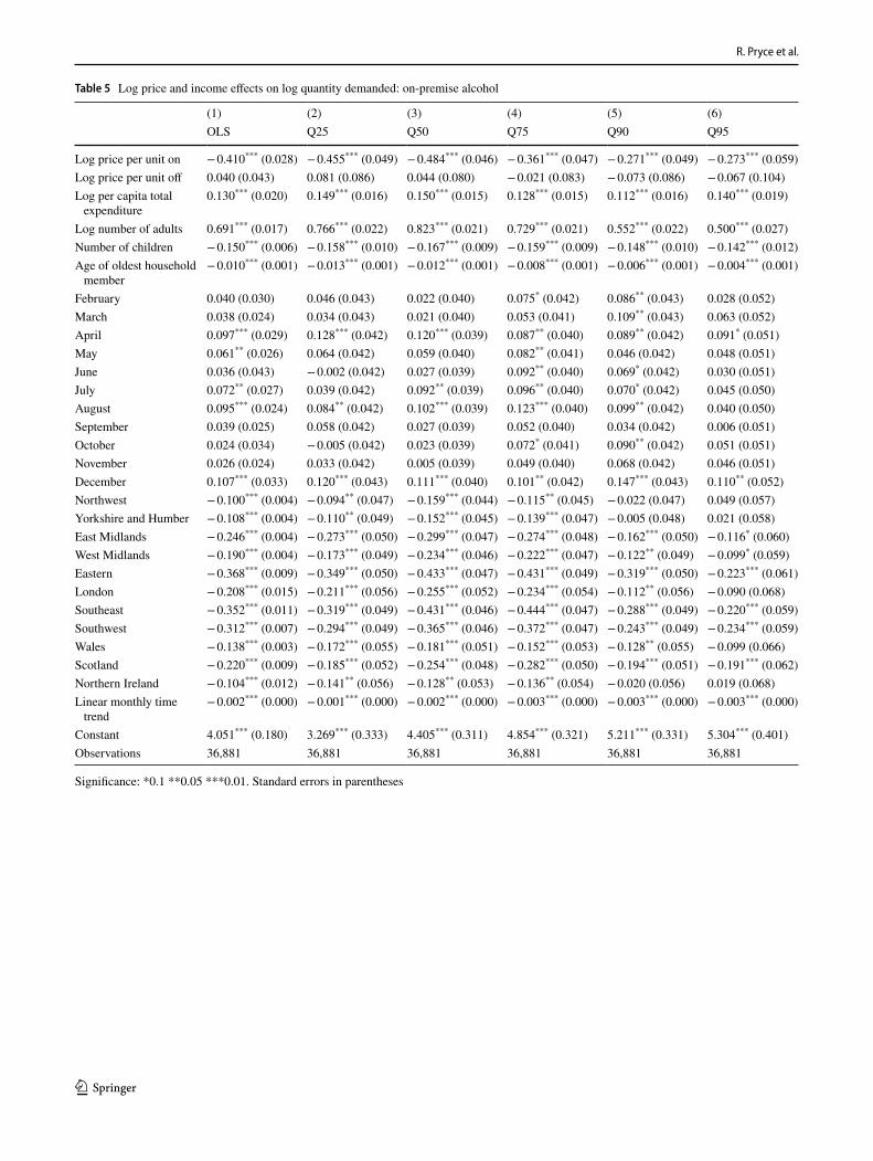
Table 5 Log price and income efects on log quantity demanded: on-premise alcohol


(1) (2) (3) (4) (5) (6)

OLS Q25 Q50 Q75 Q90 Q95

Log price per unit on − 0.410*** (0.028) − 0.455*** (0.049) − 0.484*** (0.046) − 0.361*** (0.047) − 0.271*** (0.049) − 0.273*** (0.059)

Log price per unit of 0.040 (0.043) 0.081 (0.086) 0.044 (0.080) − 0.021 (0.083) − 0.073 (0.086) − 0.067 (0.104)


0.130*** (0.020) 0.149*** (0.016) 0.150*** (0.015) 0.128*** (0.015) 0.112*** (0.016) 0.140*** (0.019)




− 0.010*** (0.001) − 0.013*** (0.001) − 0.012*** (0.001) − 0.008*** (0.001) − 0.006*** (0.001) − 0.004*** (0.001)

February 0.040 (0.030) 0.046 (0.043) 0.022 (0.040) 0.075* (0.042) 0.086** (0.043) 0.028 (0.052)

March 0.038 (0.024) 0.034 (0.043) 0.021 (0.040) 0.053 (0.041) 0.109** (0.043) 0.063 (0.052)

April 0.097*** (0.029) 0.128*** (0.042) 0.120*** (0.039) 0.087** (0.040) 0.089** (0.042) 0.091* (0.051)

May 0.061** (0.026) 0.064 (0.042) 0.059 (0.040) 0.082** (0.041) 0.046 (0.042) 0.048 (0.051)

June 0.036 (0.043) − 0.002 (0.042) 0.027 (0.039) 0.092** (0.040) 0.069* (0.042) 0.030 (0.051)

July 0.072** (0.027) 0.039 (0.042) 0.092** (0.039) 0.096** (0.040) 0.070* (0.042) 0.045 (0.050)

August 0.095*** (0.024) 0.084** (0.042) 0.102*** (0.039) 0.123*** (0.040) 0.099** (0.042) 0.040 (0.050)

September 0.039 (0.025) 0.058 (0.042) 0.027 (0.039) 0.052 (0.040) 0.034 (0.042) 0.006 (0.051)

October 0.024 (0.034) − 0.005 (0.042) 0.023 (0.039) 0.072* (0.041) 0.090** (0.042) 0.051 (0.051)

November 0.026 (0.024) 0.033 (0.042) 0.005 (0.039) 0.049 (0.040) 0.068 (0.042) 0.046 (0.051)

December 0.107*** (0.033) 0.120*** (0.043) 0.111*** (0.040) 0.101** (0.042) 0.147*** (0.043) 0.110** (0.052)

Northwest − 0.100*** (0.004) − 0.094** (0.047) − 0.159*** (0.044) − 0.115** (0.045) − 0.022 (0.047) 0.049 (0.057)

Yorkshire and Humber − 0.108*** (0.004) − 0.110** (0.049) − 0.152*** (0.045) − 0.139*** (0.047) − 0.005 (0.048) 0.021 (0.058)

East Midlands − 0.246*** (0.004) − 0.273*** (0.050) − 0.299*** (0.047) − 0.274*** (0.048) − 0.162*** (0.050) − 0.116* (0.060)

West Midlands − 0.190*** (0.004) − 0.173*** (0.049) − 0.234*** (0.046) − 0.222*** (0.047) − 0.122** (0.049) − 0.099* (0.059)

Eastern − 0.368*** (0.009) − 0.349*** (0.050) − 0.433*** (0.047) − 0.431*** (0.049) − 0.319*** (0.050) − 0.223*** (0.061)

London − 0.208*** (0.015) − 0.211*** (0.056) − 0.255*** (0.052) − 0.234*** (0.054) − 0.112** (0.056) − 0.090 (0.068)

Southeast − 0.352*** (0.011) − 0.319*** (0.049) − 0.431*** (0.046) − 0.444*** (0.047) − 0.288*** (0.049) − 0.220*** (0.059)

Southwest − 0.312*** (0.007) − 0.294*** (0.049) − 0.365*** (0.046) − 0.372*** (0.047) − 0.243*** (0.049) − 0.234*** (0.059)

Wales − 0.138*** (0.003) − 0.172*** (0.055) − 0.181*** (0.051) − 0.152*** (0.053) − 0.128** (0.055) − 0.099 (0.066)

Scotland − 0.220*** (0.009) − 0.185*** (0.052) − 0.254*** (0.048) − 0.282*** (0.050) − 0.194*** (0.051) − 0.191*** (0.062)

Northern Ireland − 0.104*** (0.012) − 0.141** (0.056) − 0.128** (0.053) − 0.136** (0.054) − 0.020 (0.056) 0.019 (0.068)


− 0.002*** (0.000) − 0.001*** (0.000) − 0.002*** (0.000) − 0.003*** (0.000) − 0.003*** (0.000) − 0.003*** (0.000)

Constant 4.051*** (0.180) 3.269*** (0.333) 4.405*** (0.311) 4.854*** (0.321) 5.211*** (0.331) 5.304*** (0.401)

Observations 36,881 36,881 36,881 36,881 36,881 36,881


1 3

Table 6 Log price and income efects on log quantity demanded: of-premise alcohol


(1) (2) (3) (4) (5) (6)

OLS Q25 Q50 Q75 Q90 Q95

Log price per unit on 0.041** (0.018) 0.060 (0.044) 0.050 (0.038) − 0.029 (0.037) − 0.000 (0.041) 0.036 (0.047)

Log price per unit of − 0.657*** (0.066) − 0.881*** (0.079) − 0.727*** (0.068) − 0.460*** (0.066) − 0.325*** (0.073) − 0.222*** (0.083)


0.311*** (0.013) 0.322*** (0.014) 0.340*** (0.012) 0.342*** (0.012) 0.304*** (0.013) 0.286*** (0.014)


Number of children − 0.016* (0.008) − 0.018** (0.009) − 0.016** (0.008) − 0.013* (0.007) − 0.015* (0.008) − 0.019** (0.009)


0.005*** (0.001) 0.005*** (0.001) 0.006*** (0.000) 0.007*** (0.000) 0.008*** (0.001) 0.007*** (0.001)

February 0.111*** (0.030) 0.164*** (0.041) 0.116*** (0.036) 0.117*** (0.035) 0.120*** (0.038) 0.050 (0.043)

March 0.086** (0.030) 0.118*** (0.040) 0.100*** (0.035) 0.082** (0.034) 0.085** (0.037) 0.003 (0.043)

April 0.082*** (0.023) 0.130*** (0.040) 0.096*** (0.034) 0.106*** (0.033) 0.076** (0.036) − 0.044 (0.042)

May 0.090*** (0.018) 0.140*** (0.040) 0.093*** (0.034) 0.096*** (0.033) 0.135*** (0.036) 0.077* (0.042)

June 0.119*** (0.020) 0.182*** (0.039) 0.120*** (0.034) 0.110*** (0.033) 0.108*** (0.036) 0.052 (0.041)

July 0.103*** (0.025) 0.119*** (0.039) 0.115*** (0.034) 0.098*** (0.033) 0.109*** (0.036) 0.039 (0.041)

August 0.096*** (0.025) 0.122*** (0.039) 0.098*** (0.034) 0.092*** (0.033) 0.116*** (0.036) 0.014 (0.041)

September 0.063*** (0.017) 0.068* (0.039) 0.089*** (0.034) 0.074** (0.033) 0.088** (0.036) − 0.007 (0.042)

October 0.102*** (0.028) 0.119*** (0.039) 0.116*** (0.034) 0.096*** (0.033) 0.105*** (0.036) − 0.006 (0.041)

November 0.221*** (0.024) 0.257*** (0.038) 0.226*** (0.033) 0.209*** (0.032) 0.256*** (0.035) 0.188*** (0.040)

December 0.376*** (0.029) 0.442*** (0.039) 0.396*** (0.033) 0.376*** (0.032) 0.389*** (0.035) 0.295*** (0.041)

Northwest 0.037*** (0.005) 0.040 (0.044) 0.048 (0.038) 0.056 (0.037) 0.030 (0.040) − 0.008 (0.046)

Yorkshire and Humber − 0.016*** (0.005) − 0.020 (0.046) − 0.020 (0.039) − 0.017 (0.038) − 0.028 (0.042) − 0.030 (0.048)

East Midlands − 0.055*** (0.005) − 0.094** (0.047) − 0.078* (0.040) − 0.067* (0.039) − 0.022 (0.043) 0.000 (0.049)

West Midlands − 0.068*** (0.005) − 0.088* (0.046) − 0.053 (0.039) − 0.044 (0.038) − 0.011 (0.042) − 0.031 (0.048)

Eastern − 0.104*** (0.010) − 0.131*** (0.047) − 0.111*** (0.040) − 0.097** (0.039) − 0.074* (0.043) − 0.079 (0.049)

London − 0.136*** (0.016) − 0.166*** (0.052) − 0.169*** (0.045) − 0.136*** (0.044) − 0.115** (0.048) − 0.130** (0.055)

Southeast − 0.075*** (0.012) − 0.081* (0.045) − 0.090** (0.039) − 0.085** (0.038) − 0.052 (0.042) − 0.052 (0.048)

Southwest − 0.056*** (0.008) − 0.055 (0.045) − 0.072* (0.039) − 0.057 (0.038) − 0.077* (0.042) − 0.094* (0.048)

Wales − 0.030*** (0.004) − 0.048 (0.051) − 0.016 (0.044) − 0.020 (0.043) 0.002 (0.047) − 0.026 (0.054)

Scotland 0.037*** (0.008) 0.042 (0.047) 0.046 (0.041) 0.039 (0.040) 0.048 (0.044) 0.012 (0.050)

Northern Ireland 0.038*** (0.011) 0.069 (0.053) 0.045 (0.046) 0.056 (0.044) − 0.012 (0.049) − 0.042 (0.056)


− 0.000*** (0.000) − 0.001*** (0.000) − 0.000*** (0.000) − 0.000** (0.000) − 0.000* (0.000) 0.000 (0.000)

Constant 3.363*** (0.230) 3.238*** (0.304) 3.411*** (0.263) 3.501*** (0.256) 3.625*** (0.280) 3.614*** (0.321)

Observations 41,572 41,572 41,572 41,572 41,572 41,572

R. Pryce et al.

1 3

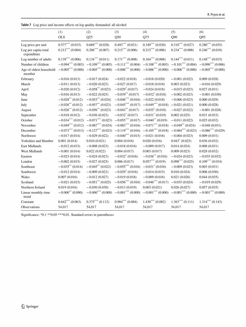
Table 7 Log price and income efects on log quality demanded: all alcohol


(1) (2) (3) (4) (5) (6)

OLS Q25 Q50 Q75 Q90 Q95

Log price per unit 0.577*** (0.015) 0.689*** (0.028) 0.493*** (0.021) 0.349*** (0.020) 0.310*** (0.027) 0.280*** (0.035)


0.213*** (0.004) 0.206*** (0.007) 0.215*** (0.006) 0.215*** (0.006) 0.234*** (0.008) 0.246*** (0.010)




− 0.005*** (0.000) − 0.005*** (0.000) − 0.006*** (0.000) − 0.006*** (0.000) − 0.006*** (0.000) − 0.005*** (0.000)

February − 0.016 (0.013) − 0.017 (0.024) − 0.022 (0.018) − 0.018 (0.020) − 0.001 (0.022) 0.009 (0.028)

March − 0.011 (0.013) − 0.020 (0.023) − 0.027 (0.017) − 0.018 (0.018) 0.003 (0.023) − 0.016 (0.029)

April − 0.020 (0.012) − 0.058** (0.023) − 0.029* (0.017) − 0.024 (0.018) − 0.015 (0.023) 0.027 (0.031)

May − 0.016 (0.013) − 0.022 (0.025) − 0.039** (0.017) − 0.032* (0.018) − 0.002 (0.023) − 0.001 (0.030)

June − 0.028** (0.012) − 0.053** (0.024) − 0.046*** (0.016) − 0.022 (0.018) − 0.006 (0.023) 0.000 (0.029)

July − 0.026** (0.012) − 0.057** (0.023) − 0.045*** (0.017) − 0.049*** (0.018) − 0.021 (0.021) 0.000 (0.028)

August − 0.026** (0.012) − 0.056** (0.023) − 0.043** (0.017) − 0.035* (0.018) − 0.027 (0.022) − 0.001 (0.028)

September − 0.018 (0.012) − 0.036 (0.023) − 0.032* (0.017) − 0.031* (0.019) 0.002 (0.025) 0.031 (0.033)

October − 0.034*** (0.012) − 0.071*** (0.023) − 0.055*** (0.017) − 0.040** (0.019) − 0.011 (0.022) 0.025 (0.032)

November − 0.049*** (0.012) − 0.087*** (0.024) − 0.083*** (0.016) − 0.071*** (0.018) − 0.049** (0.024) − 0.048 (0.031)

December − 0.073*** (0.013) − 0.127*** (0.023) − 0.119*** (0.016) − 0.105*** (0.018) − 0.084*** (0.023) − 0.086*** (0.029)

Northwest − 0.017 (0.014) − 0.029 (0.022) − 0.040*** (0.015) − 0.021 (0.016) − 0.004 (0.023) 0.009 (0.031)

Yorkshire and Humber 0.001 (0.014) 0.010 (0.021) 0.004 (0.016) 0.020 (0.016) 0.043* (0.025) 0.036 (0.032)

East Midlands − 0.012 (0.015) − 0.008 (0.023) − 0.018 (0.016) − 0.009 (0.017) 0.014 (0.024) 0.008 (0.031)

West Midlands − 0.001 (0.014) 0.022 (0.022) 0.004 (0.017) 0.003 (0.017) 0.009 (0.023) 0.028 (0.032)

Eastern − 0.023 (0.014) − 0.024 (0.023) − 0.032* (0.016) − 0.036** (0.016) − 0.024 (0.023) − 0.035 (0.032)

London − 0.002 (0.015) − 0.027 (0.025) 0.006 (0.017) 0.057*** (0.019) 0.098*** (0.025) 0.109*** (0.034)

Southeast − 0.035** (0.014) − 0.045** (0.022) − 0.055*** (0.016) − 0.031* (0.016) − 0.009 (0.023) 0.003 (0.031)

Southwest − 0.012 (0.014) − 0.009 (0.023) − 0.029* (0.016) − 0.014 (0.015) 0.010 (0.024) 0.006 (0.030)

Wales 0.007 (0.016) − 0.012 (0.027) − 0.019 (0.018) − 0.009 (0.016) 0.021 (0.026) 0.044 (0.035)

Scotland − 0.021 (0.015) − 0.051** (0.025) − 0.056*** (0.016) − 0.046*** (0.017) − 0.035 (0.024) − 0.019 (0.029)

Northern Ireland 0.019 (0.016) − 0.030 (0.030) − 0.013 (0.019) 0.003 (0.021) 0.026 (0.027) 0.057 (0.035)


− 0.000** (0.000) − 0.000*** (0.000) − 0.001*** (0.000) − 0.001*** (0.000) − 0.001*** (0.000) − 0.001*** (0.000)

Constant 0.642*** (0.063) 0.375*** (0.112) 0.984*** (0.084) 1.430*** (0.082) 1.363*** (0.111) 1.314*** (0.143)

Observations 54,017 54,017 54,017 54,017 54,017 54,017


1 3

Table 8 Log price and income efects on log quality demanded: on-premise alcohol


(1) (2) (3) (4) (5) (6)

OLS Q25 Q50 Q75 Q90 Q95

Log price per unit on 0.601*** (0.014) 0.427*** (0.015) 0.311*** (0.013) 0.233*** (0.013) 0.176*** (0.017) 0.176*** (0.017)

Log price per unit of − 0.021 (0.025) 0.009 (0.025) 0.027 (0.020) 0.050** (0.020) 0.030 (0.028) 0.023 (0.030)


0.197*** (0.005) 0.158*** (0.005) 0.164*** (0.004) 0.166*** (0.004) 0.171*** (0.005) 0.179*** (0.005)




− 0.002*** (0.000) − 0.002*** (0.000) − 0.002*** (0.000) − 0.002*** (0.000) − 0.002*** (0.000) − 0.002*** (0.000)

February − 0.013 (0.012) 0.005 (0.012) − 0.009 (0.010) − 0.012 (0.009) − 0.030** (0.013) − 0.055*** (0.017)

March − 0.012 (0.012) 0.011 (0.012) 0.004 (0.009) − 0.003 (0.010) − 0.030** (0.014) − 0.028* (0.015)

April − 0.010 (0.012) − 0.007 (0.011) 0.001 (0.009) − 0.007 (0.009) − 0.030** (0.014) − 0.025* (0.015)

May − 0.010 (0.012) − 0.007 (0.011) − 0.008 (0.009) − 0.020** (0.009) − 0.033** (0.013) − 0.027** (0.013)

June − 0.022* (0.012) − 0.016 (0.011) − 0.018** (0.009) − 0.020** (0.009) − 0.025** (0.013) − 0.031** (0.013)

July − 0.020* (0.012) − 0.017 (0.011) − 0.014 (0.010) − 0.016* (0.009) − 0.033** (0.014) − 0.043*** (0.014)

August − 0.021* (0.012) 0.003 (0.011) − 0.007 (0.009) − 0.018* (0.009) − 0.029** (0.013) − 0.029** (0.014)

September − 0.010 (0.012) − 0.003 (0.010) − 0.005 (0.009) − 0.010 (0.010) − 0.017 (0.012) − 0.014 (0.013)

October − 0.015 (0.012) − 0.010 (0.011) − 0.021** (0.009) − 0.024*** (0.009) − 0.037*** (0.013) − 0.037** (0.015)

November − 0.013 (0.012) 0.008 (0.013) − 0.007 (0.010) − 0.020** (0.009) − 0.033*** (0.013) − 0.031* (0.016)

December − 0.014 (0.012) 0.012 (0.013) 0.009 (0.010) − 0.007 (0.010) − 0.019 (0.013) − 0.038*** (0.013)

Northwest 0.002 (0.014) 0.005 (0.012) 0.023** (0.010) 0.035*** (0.012) 0.033* (0.018) 0.035** (0.018)

Yorkshire and Humber − 0.004 (0.014) − 0.005 (0.012) 0.009 (0.010) 0.020* (0.012) 0.027 (0.018) 0.037** (0.017)

East Midlands 0.020 (0.014) 0.012 (0.013) 0.037*** (0.011) 0.057*** (0.012) 0.070*** (0.017) 0.094*** (0.015)

West Midlands 0.020 (0.014) 0.019 (0.011) 0.039*** (0.011) 0.053*** (0.012) 0.053*** (0.017) 0.068*** (0.016)

Eastern 0.028* (0.015) 0.043*** (0.014) 0.081*** (0.012) 0.113*** (0.013) 0.133*** (0.018) 0.150*** (0.017)

London 0.040** (0.016) 0.099*** (0.018) 0.135*** (0.014) 0.160*** (0.016) 0.165*** (0.022) 0.180*** (0.021)

Southeast 0.027* (0.014) 0.055*** (0.013) 0.102*** (0.011) 0.136*** (0.013) 0.145*** (0.019) 0.154*** (0.018)

Southwest 0.031** (0.014) 0.038*** (0.013) 0.077*** (0.011) 0.102*** (0.012) 0.115*** (0.018) 0.135*** (0.017)

Wales 0.028* (0.016) 0.034** (0.015) 0.046*** (0.012) 0.059*** (0.013) 0.073*** (0.020) 0.071*** (0.015)

Scotland 0.048*** (0.015) 0.073*** (0.017) 0.103*** (0.013) 0.121*** (0.015) 0.118*** (0.019) 0.117*** (0.021)

Northern Ireland 0.079*** (0.016) 0.141*** (0.016) 0.161*** (0.016) 0.152*** (0.016) 0.140*** (0.023) 0.132*** (0.021)


0.000*** (0.000) 0.001*** (0.000) 0.001*** (0.000) 0.001*** (0.000) 0.001*** (0.000) 0.001*** (0.000)

Constant 0.745*** (0.096) 1.516*** (0.091) 1.864*** (0.080) 2.066*** (0.079) 2.305*** (0.106) 2.265*** (0.114)

Observations 36,839 36,839 36,839 36,839 36,839 36,839

R. Pryce et al.

1 3

Table 9 Log price and income efects on log quality demanded: of-premise


(1) (2) (3) (4) (5) (6)

OLS Q25 Q50 Q75 Q90 Q95

Log price per unit on − 0.022** (0.010) − 0.018 (0.013) − 0.024** (0.010) − 0.028** (0.011) − 0.021 (0.014) − 0.014 (0.020)

Log price per unit of 0.775*** (0.018) 0.730*** (0.023) 0.611*** (0.018) 0.541*** (0.021) 0.498*** (0.027) 0.461*** (0.036)


0.134*** (0.003) 0.112*** (0.004) 0.124*** (0.003) 0.140*** (0.004) 0.150*** (0.005) 0.159*** (0.006)

Log number of adults 0.033*** (0.005) 0.012** (0.006) 0.024*** (0.005) 0.031*** (0.005) 0.036*** (0.007) 0.034*** (0.009)



− 0.001*** (0.000) − 0.002*** (0.000) − 0.002*** (0.000) − 0.001*** (0.000) − 0.001*** (0.000) − 0.001*** (0.000)

February − 0.004 (0.009) − 0.005 (0.012) − 0.008 (0.010) − 0.016 (0.010) − 0.010 (0.015) − 0.015 (0.019)

March 0.003 (0.009) − 0.004 (0.012) 0.001 (0.008) − 0.010 (0.010) − 0.005 (0.013) − 0.020 (0.016)

April − 0.004 (0.009) − 0.013 (0.012) − 0.005 (0.008) − 0.013 (0.010) − 0.012 (0.014) − 0.031* (0.016)

May 0.001 (0.009) 0.008 (0.012) − 0.003 (0.009) − 0.010 (0.010) − 0.018 (0.013) − 0.021 (0.018)

June − 0.003 (0.009) 0.003 (0.012) 0.001 (0.009) − 0.002 (0.010) − 0.020 (0.015) − 0.026 (0.017)

July − 0.005 (0.009) − 0.013 (0.012) − 0.006 (0.009) − 0.015 (0.011) − 0.009 (0.013) − 0.020 (0.016)

August − 0.006 (0.009) − 0.002 (0.012) − 0.008 (0.009) − 0.017* (0.010) − 0.011 (0.012) − 0.024 (0.016)

September 0.000 (0.009) − 0.011 (0.012) − 0.005 (0.008) − 0.006 (0.010) − 0.001 (0.014) − 0.012 (0.019)

October 0.001 (0.009) − 0.003 (0.012) − 0.001 (0.008) − 0.010 (0.010) − 0.017 (0.015) − 0.031** (0.015)

November − 0.008 (0.009) − 0.014 (0.012) − 0.018** (0.008) − 0.018* (0.010) − 0.013 (0.013) − 0.014 (0.018)

December − 0.017* (0.009) − 0.018 (0.013) − 0.018** (0.008) − 0.013 (0.010) − 0.010 (0.013) − 0.037** (0.017)

Northwest − 0.007 (0.010) − 0.008 (0.011) − 0.004 (0.009) 0.000 (0.009) 0.011 (0.013) − 0.015 (0.019)

Yorkshire and Humber − 0.004 (0.010) − 0.006 (0.012) 0.000 (0.009) 0.004 (0.010) 0.012 (0.013) − 0.008 (0.020)

East Midlands − 0.007 (0.010) 0.003 (0.012) 0.007 (0.009) 0.015 (0.009) 0.023 (0.014) 0.005 (0.020)

West Midlands − 0.001 (0.010) 0.003 (0.012) 0.003 (0.010) 0.002 (0.010) − 0.003 (0.015) − 0.018 (0.018)

Eastern − 0.009 (0.010) − 0.001 (0.011) 0.007 (0.010) 0.011 (0.010) 0.023 (0.014) 0.012 (0.022)

London − 0.005 (0.012) 0.002 (0.014) 0.032*** (0.011) 0.051*** (0.012) 0.063*** (0.018) 0.059** (0.024)

Southeast − 0.016 (0.010) − 0.009 (0.012) 0.006 (0.010) 0.013 (0.010) 0.022 (0.015) − 0.005 (0.020)

Southwest − 0.005 (0.010) − 0.007 (0.011) 0.002 (0.009) 0.012 (0.010) 0.024* (0.013) 0.006 (0.019)

Wales 0.003 (0.011) − 0.002 (0.013) 0.001 (0.011) 0.007 (0.012) 0.013 (0.017) − 0.011 (0.021)

Scotland 0.008 (0.011) 0.001 (0.012) 0.013 (0.010) 0.018* (0.011) 0.026* (0.014) − 0.006 (0.020)

Northern Ireland 0.020* (0.012) 0.040*** (0.015) 0.046*** (0.011) 0.045*** (0.011) 0.058*** (0.016) 0.044* (0.023)


0.000*** (0.000) 0.000* 0.000** 0.000 − 0.000 0.000

(0.000) (0.000) (0.000) (0.000) (0.000)

Constant 0.155** (0.068) 0.453*** (0.089) 0.724*** (0.070) 0.823*** (0.077) 0.822*** (0.104) 0.857*** (0.138)

Observations 41,487 41,487 41,487 41,487 41,487 41,487


1 3

References

1. HMRC: Alcohol Factsheet. Her Majesty’s Revenue and Customs, London (2012)

2. WHO: Global Status Report on Alcohol and Health. World Health Organization, New York (2011)

3. ONS: Adult Drinking Habits in Great Britain. Oice for National Statistics, London (2016)

4. Di Castelnuovo, A., Costanzo, S., Bagnardi, V., Donati, M.B., Iacoviello, L., De Gaetano, G.: Alcohol dosing and total mortality in men and women: an updated meta-analysis of 34 prospective studies. Arch. Intern. Med. 166(22), 2437–2445 (2006)

5. Rehm, J., Taylor, B., Mohapatra, S., Irving, H., Baliunas, D., Patra, J., Roerecke, M.: Alcohol as a risk factor for liver cirrhosis: a systematic review and meta-analysis. Drug Alcohol Rev. 29(4), 437–445 (2010)

6. Tramacere, I., Negri, E., Bagnardi, V., Garavello, W., Rota, M., Scotti, L., Islami, F., Corrao, G., Bofetta, P., La Vecchia, C.: A meta-analysis of alcohol drinking and oral and pharyngeal can-cers. Part 1: overall results and dose-risk relation. Oral Oncol. 46(7), 497–503 (2010)

7. Elkind, M.S., Sciacca, R., Boden-Albala, B., Rundek, T., Paik, M.C., Sacco, R.L.: Moderate alcohol consumption reduces risk of ischemic stroke: the Northern Manhattan study. Stroke 37(1), 13–19 (2006)

8. Fillmore, K.M., Stockwell, T., Chikritzhs, T., Bostrom, A., Kerr, W.: Moderate alcohol use and reduced mortality risk: systematic error in prospective studies and new hypotheses. Ann. Epidemiol. 17(5), S16–S23 (2007)

9. Knott, C.S., Coombs, N., Stamatakis, E., Biddulph, J.P.: All cause mortality and the case for age speciic alcohol consumption guide-lines: pooled analyses of up to 10 population based cohorts. BMJ 350, h384 (2015)

Table 10 Log price and income efects on log quantity demanded: all alcohol (robustness check, monthly price)


(1) (2) (3) (4) (5) (6)

OLS Q25 Q50 Q75 Q90 Q95

Log price per unit − 0.570*** (0.071) − 0.762*** (0.155) − 0.560*** (0.116) − 0.423*** (0.101) − 0.314*** (0.108) − 0.272** (0.130)


0.338*** (0.014) 0.349*** (0.015) 0.385*** (0.011) 0.380*** (0.010) 0.336*** (0.010) 0.322*** (0.013)




− 0.000 (0.001) − 0.003*** (0.001) 0.001 (0.000) 0.002*** (0.000) 0.004*** (0.000) 0.004*** (0.001)

February 0.098*** (0.018) 0.125*** (0.043) 0.110*** (0.032) 0.117*** (0.028) 0.118*** (0.030) 0.097*** (0.036)

March 0.101*** (0.031) 0.106** (0.043) 0.124*** (0.032) 0.121*** (0.028) 0.107*** (0.030) 0.073** (0.036)

April 0.137*** (0.018) 0.159*** (0.042) 0.165*** (0.031) 0.155*** (0.028) 0.106*** (0.029) 0.027 (0.035)

May 0.122*** (0.021) 0.140*** (0.043) 0.126*** (0.032) 0.123*** (0.028) 0.126*** (0.030) 0.107*** (0.036)

June 0.139*** (0.032) 0.190*** (0.043) 0.158*** (0.032) 0.135*** (0.028) 0.142*** (0.030) 0.104*** (0.036)

July 0.148*** (0.018) 0.190*** (0.042) 0.154*** (0.032) 0.123*** (0.028) 0.127*** (0.029) 0.115*** (0.035)

August 0.151*** (0.017) 0.176*** (0.042) 0.152*** (0.032) 0.135*** (0.028) 0.145*** (0.030) 0.079** (0.035)

September 0.098** (0.033) 0.133*** (0.042) 0.102*** (0.031) 0.098*** (0.027) 0.109*** (0.029) 0.044 (0.035)

October 0.112*** (0.029) 0.148*** (0.043) 0.137*** (0.032) 0.118*** (0.028) 0.124*** (0.030) 0.051 (0.036)

November 0.219*** (0.026) 0.251*** (0.044) 0.230*** (0.033) 0.211*** (0.029) 0.223*** (0.031) 0.194*** (0.037)

December 0.378*** (0.042) 0.445*** (0.047) 0.402*** (0.035) 0.339*** (0.031) 0.343*** (0.033) 0.314*** (0.040)

Northwest − 0.041*** (0.002) − 0.079* (0.047) − 0.038 (0.035) 0.030 (0.031) − 0.007 (0.033) 0.003 (0.039)

Yorkshire and Humber − 0.085*** (0.001) − 0.137*** (0.049) − 0.095*** (0.036) − 0.033 (0.032) − 0.041 (0.034) − 0.025 (0.041)

East Midlands − 0.150*** (0.002) − 0.214*** (0.050) − 0.181*** (0.037) − 0.124*** (0.033) − 0.072** (0.035) − 0.048 (0.042)

West Midlands − 0.166*** (0.002) − 0.284*** (0.049) − 0.155*** (0.036) − 0.133*** (0.032) − 0.078** (0.034) − 0.051 (0.041)

Eastern − 0.302*** (0.004) − 0.404*** (0.049) − 0.329*** (0.036) − 0.243*** (0.032) − 0.175*** (0.034) − 0.122*** (0.041)

London − 0.351*** (0.004) − 0.465*** (0.050) − 0.396*** (0.037) − 0.283*** (0.032) − 0.226*** (0.035) − 0.192*** (0.042)

Southeast − 0.297*** (0.005) − 0.396*** (0.046) − 0.336*** (0.034) − 0.233*** (0.030) − 0.178*** (0.032) − 0.113*** (0.038)

Southwest − 0.216*** (0.003) − 0.275*** (0.048) − 0.237*** (0.036) − 0.159*** (0.032) − 0.155*** (0.034) − 0.130*** (0.040)

Wales − 0.085*** (0.001) − 0.123** (0.055) − 0.120*** (0.041) − 0.065* (0.036) − 0.034 (0.038) − 0.029 (0.046)

Scotland − 0.115*** (0.002) − 0.139*** (0.049) − 0.128*** (0.037) − 0.074** (0.032) − 0.056 (0.034) − 0.043 (0.041)

Northern Ireland − 0.193*** (0.004) − 0.264*** (0.052) − 0.219*** (0.039) − 0.117*** (0.034) − 0.142*** (0.036) − 0.105** (0.043)


− 0.001*** (0.000) − 0.002*** (0.000) − 0.001*** (0.000) − 0.001*** (0.000) − 0.001*** (0.000) − 0.001*** (0.000)

Constant 3.815*** (0.320) 3.909*** (0.598) 3.655*** (0.445) 3.720*** (0.389) 3.970*** (0.417) 4.146*** (0.500)

Observations 54,069 54,069 54,069 54,069 54,069 54,069

R. Pryce et al.

1 3

10. Becker, G.S., Murphy, K.M.: Murphy. A theory of rational addic-tion. J. Political Econ. 96(4), 675–700 (1988)

11. Ludbrook, A.: Minimum pricing of alcohol. Health Econ. 18(12), 1357–1360 (2009)

12. Brennan, A., Meng, Y., Holmes, J., Hill-McManus, D., Meier, P.S.: Potential beneits of minimum unit pricing for alcohol versus a ban on below cost selling in England 2014: modelling study. BMJ 349(302), g5452 (2014)

13. Meng, Y., Brennan, A., Purshouse, R., Hill-McManus, D., Angus, C., Holmes, J., Meier, P.S.: Estimation of own and cross-price elasticities of alcohol demand in the UK: a pseudo-panel approach using the living costs and food survey 2001–2009. J. Health Econ. 4, 96–103 (2014)

14. Gallet, C.A.: The demand for alcohol: a meta-analysis of elastici-ties. Aust. J. Agric. Resour. Econ. 51(2), 121–135 (2007)

15. Wagenaar, A.C., Salois, M.J., Komro, K.A.: Efect of beverage alcohol price and tax levels on drinking: a meta-analysis of 1003 estimates from 112 studies. Addiction 104(2), 179–190 (2009)

16. Purshouse, R., Meier, P.S., Brennan, A., Taylor, K.B., Raia, R.: Estimated efect of alcohol pricing policies on health and health economic outcomes in England: an epidemiological model. Lan-cet 375(9723), 1355–1364 (2010)

17. Koenker, R., Hallock, K.: Quantile regression: an introduction. J. Econ. Perspect. 15(4), 43–56 (2001)

18. Manning, W.G., Blumberg, L., Moulton, L.H.: The demand for alcohol: the diferential response to price. J. Health Econ. 14(2), 123–148 (1995)

19. Safer, H., Dave, D., Grossman, M.: A behavioural economic model of alcohol advertising and price. Health Econ. 25(7), 816–828 (2016)

20. Byrnes, J., Shakeshaft, A., Petrie, D., Doran, C.M.: Is response to price equal for those with higher alcohol consumption? Eur. J. Health Econ. 17(1), 23–29 (2016)

21. Gruenewald, P.J., Ponicki, W.R., Holder, H.D., Romelsjö, A.: Alcohol prices, beverage quality, and the demand for alcohol: quality substitutions and price elasticities. Alcohol. Clin. Exp. Res. 30(1), 96–105 (2006)

22. Firpo, S., Fortin, N.M., Lemieux, T.: Unconditional quantile regressions. Econometrica 77(3), 953–973 (2009)

23. Borah, B.J., Basu, A.: Highlighting diferences between condi-tional and unconditional quantile regression approaches through an application to assess medication adherence. Health Econ. 22(9), 1052–1070 (2013)

24. Deaton, A.: Quality, quantity, and spatial variation of price. Am. Econ. Rev. 78(3), 418–430 (1988)

25. Prais, S.J., Houthakker, H.S.: The Analysis of Family Budgets. Cambridge University Press, New York (1955)

26. Gibson, J., Kim, B.: Testing the infrequent purchases model using direct measurement of hidden consumption from food stocks. Am. J. Agric. Econ. 94(1), 257–270 (2012)

27. Boniface, S., Shelton, N.: How is alcohol consumption afected if we account for under-reporting? a hypothetical scenario. Eur. J. Pub. Health 23(6), 1076–1081 (2013)

alcohol quantity and quality price elasticities: quantile...

Documents