akdeniz erol 2003

8/13/2019 Akdeniz Erol 2003

http://slidepdf.com/reader/full/akdeniz-erol-2003 1/27

This article was downloaded by:[ANKOS Consortium]On: 25 January 2008

Access Details: [subscription number 772815469]Publisher: Taylor & FrancisInforma Ltd Registered in England and Wales Registered Number: 1072954Registered office: Mortimer House, 37-41 Mortimer Street, London W1T 3JH, UK

Communications in Statistics -Theory and MethodsPublication details, including instructions for authors and subscription information:http://www.informaworld.com/smpp/title~content=t713597238

Mean Squared Error Matrix Comparisons of SomeBiased Estimators in Linear RegressionFikri Akdeniz a ; Hamza Erol aa Department of Statistics, Faculty of Arts and Sciences, University of Çukurova,

Adana, Turkey

Online Publication Date: 12 January 2003To cite this Article: Akdeniz, Fikri and Erol, Hamza (2003) 'Mean Squared Error

Matrix Comparisons of Some Biased Estimators in Linear Regression',Communications in Statistics - Theory and Methods, 32:12, 2389 - 2413To link to this article: DOI: 10.1081/STA-120025385

URL: http://dx.doi.org/10.1081/STA-120025385

PLEASE SCROLL DOWN FOR ARTICLE

Full terms and conditions of use: http://www.informaworld.com/terms-and-conditions-of-access.pdf

This article maybe used for research, teaching and private study purposes. Any substantial or systematic reproduction,re-distribution, re-selling, loan or sub-licensing, systematic supply or distribution in any form to anyone is expresslyforbidden.

The publisher does not give any warranty express or implied or make any representation that the contents will becomplete or accurate or up to date. The accuracy of any instructions, formulae and drug doses should beindependently verified with primary sources. The publisher shall not be liable for any loss, actions, claims, proceedings,demand or costs or damages whatsoever or howsoever caused arising directly or indirectly in connection with or arising out of the use of this material.

http://www.informaworld.com/smpp/title~content=t713597238

http://dx.doi.org/10.1081/STA-120025385

http://www.informaworld.com/terms-and-conditions-of-access.pdf

http://www.informaworld.com/terms-and-conditions-of-access.pdf

http://dx.doi.org/10.1081/STA-120025385

http://www.informaworld.com/smpp/title~content=t713597238



©200 3 Marcel Dekker, Inc. All rights reserved. This material may not be used or reproduced in any form without the express written permission of Marcel Dekker, Inc.

M ARCEL D EKKER, I NC . • 270 M ADISON A VENUE • N EW YORK , NY 10016

COMMUNICATIONS IN STATISTICS

Theory and MethodsVol. 32, No. 12, pp. 2389–2413, 2003

Mean Squared Error Matrix Comparisons of Some Biased Estimators in Linear Regression

Fikri Akdeniz * and Hamza Erol

Department of Statistics, Faculty of Arts and Sciences,University of C ukurova, Adana, Turkey

ABSTRACT

Consider the linear regression model y ¼ X þ u in the usual nota-tion. In the presence of multicollinearity certain biased estimators likethe ordinary ridge regression estimator ^

k ¼ ðX 0X þ kI Þ 1X 0 yand the Liu estimator ^

d ¼ ðX 0X þ I Þ 1ðX 0 y þ d ^Þ introduced by

Liu (Liu, Ke Jian. (1993). A new class of biased estimate inlinear regression. Communications in Statistics-Theory and Methods22(2):393–402) or improved ridge and Liu estimators are used to out-perform the ordinary least squares estimates in the linear regressionmodel. In this article we compare the (almost unbiased) generalizedridge regression estimator with the (almost unbiased) generalized Liuestimator in the matrix mean square error sense.

*Correspondence: Fikri Akdeniz, Department of Statistics, Faculty of Arts andSciences, University of C ukurova, 01330 Adana, Turkey; Fax: +90-322-3386070;E-mail: [email protected].

2389

DOI: 10.1081/STA-120025385 0361-0926 (Print); 1532-415X (Online)Copyright & 2003 by Marcel Dekker, Inc. www.dekker.com





Key Words: Correlation matrix; Liu estimator; Mean square error;Multicollinearity; Ridge regression estimator.

1. INTRODUCTION

The problem of multicollinearity and its statistical consequences fora linear regression model are very well-known in statistics.Multicollinearity is dened as the existence of nearly linear dependencyamong column vectors of the design matrix X in the linear model y ¼ X þ u. The best way of explaining the structure of multicollinearity

is to look over the eigenvalues and eigenvectors of the matrix X 0

X .In case of multicollinearity we know that when the correlation matrixhas one or more small eigenvalues, the estimates of the regressioncoefficients can be large in absolute value. Severe multicollinearity maymake the estimates so unstable that they are practically useless. In thissituation, the matrix X 0X becomes near singular or ill-conditioned andleast squares estimator ^ will pass undue sensitivity to the data. Toovercome this, different remedial actions have been proposed. One of biased estimators of used when collinearity is present in the data, theordinary ridge regression (ORR) estimator, is dened by

^k ¼ ðX 0X þ kI Þ 1X 0 y,

where k>0. When k ¼ 0 we have the ordinary least squares estimator ^

of . The name ridge regression was rst used by Hoerl and Kennard(1970a, 1970b).

To combat near multicollinearity, Liu (1993) combined the Stein(1956) estimator with the ORR estimator. The estimator ^

d due to Liu(1993), is called the Liu estimator by Akdeniz and Kac iranlar (1995),(see also Gruber, 1998 p. 48 and Kac iranlar et al., 1999), is dened foreach parameter d 2 ð 1 , þ 1Þ as follows:

^d :¼ ðX 0X þ I Þ 1ðX 0 y þ d ^Þ:

However, Liu (1993) did not compare the mean square error proper-ties of his estimator to that of the ORR estimator. Sakalliog lu et al.,

(2001) compared the mean square error (MSE) matrices of ^

k and ^

d .Akdeniz et al., (1999) proposed the improved Liu estimator of by forming a convex combination of the ordinary least squares (OLS)estimator and the generalized Liu estimator. The performance of theproposed estimator as compared with the generalized Liu estimator

2390 Akdeniz and Erol





and the almost unbiased generalized Liu estimator in terms of the meansquare error criterion.

In this article under review several estimators of the parameter vectorin the multiple linear regression model are compared in terms of theirrespective mean square error matrices. These include the generalizedridge regression estimator, the generalized Liu estimator, and so-calledalmost unbiased versions of these estimators. The article starts with anintroductory section containing a brief review of the literature on theseestimators. In Sec. 2 the general multiple linear regression model isdened, and expressions are provided for the estimators to be comparedin the remainder of the atricle. The mean square error matrix of anestimator is also dened in this section. In Sec. 3 two theorems arepresented and proved. These theorems establish comparative results onthe mean square error matrices of the generalized ridge regressionestimator and the generalized Liu estimator. It is important to notethat the biasing parameters in these estimators are assumed to benonstochastic to make the problem mathematically tractable in thissection. In practice, these biasing parameters are typically estimatedfrom the available data. Section 4 is largely a replicate of Sec. 3, butnow the almost unbiased generalized ridge regression estimator and thealmost unbiased generalized Liu estimator are compared in terms of theirmean square error matrices. The rst part of Sec. 5 contains a summaryof different estimates that have been proposed in the literature for thebiasing parameters of the previously discussed estimators. This isfollowed by application of the theorems of Secs. 3 and 4 to these cases.The article closes in Sec. 6 with an extensive discussion of an example.

2. THE MODEL AND ESTIMATORS

Let us consider the general linear regression model

y ¼ Z þ u ð2:1Þ

where Z is an n p matrix with full column rank of observations onnonstochastic regressors, y is an n 1 vector of observations on the depen-dent variable, isan p 1 vector of unknown regression coefficients and u

is an n 1 vector of independent and identically distributed random errorswith E (u) ¼ 0 and E ðuu0Þ ¼ 2I n.It is common practice in ridge regression to standardize the Z matrix

so that Z 0Z is in correlation form. We also standardize y so that both Z and y are in the standardized form.

MSE Matrix Comparisons 2391





It is well known that a linear regression model can be transformed toa canonical form by orthogonal transformation. Let T be an orthogonalmatrix such that

T 0Z 0ZT ¼ ð2:2Þ

where is a p p diagonal matrix whose elements 1, 2, . . . , p are theeigenvalues of Z 0Z . Making use of the matrix T , we obtain a canonicalform of the model (2.1):

y ¼ X þ u ð2:3Þ

where X :¼ ZT and :¼ T 0 . Then, working with the model (2.3) theordinary least squares estimator of is written as

^ ¼ ðX 0X Þ 1X 0 y,

or

^ ¼ 1X 0 y: ð2:4Þ

The presence of multicollinearity among regression variables in linearregression analysis may cause highly unstable least squares estimates of

the regression parameters. The statisticians thus face the problem of choosing between the least squares estimator and a biased estimator.They also face the problem of choosing between two biased estimators.The following biased estimators are considered throughout the article.

Ordinary Ridge Regression (ORR) Estimator andGeneralized Ridge Regression (GRR) Estimator

^k ¼ ð þ kI Þ 1X 0 y, k > 0 ð2:5Þ

^K ¼ ð þ K Þ 1X 0 y ¼ ð þ K Þ 1X 0X ^ ¼ ð þ K Þ 1 ^, ð2:6Þ

where K ¼ diag( k i ) is a diagonal matrix of biasing factors, ki >0,i ¼ 1,2, . . . , p, (see Hoerl and Kennard, 1970a; 1970b).






Almost Unbiased Ridge (AUR) and Almost UnbiasedGeneralized Ridge Regression (AUGRR) Estimators

ek ¼ ½I k2ð þ kI Þ 2 ^ and eK ¼ ½I ðð þ K Þ 1K Þ2 ^,ð2:7Þ

(see Singh et al., 1986).

Liu Estimator and Generalized Liu (GL) Estimator

The Liu estimator ^

d , is dened for each parameter d 2 ð 1 , 1Þ ,ðsee Kac iranlar et al., 1999) as follows:

^d ¼ ð þ I Þ 1ðX 0 y þ d ^Þ ð2:8Þ

or

^d ¼ ð þ I Þ 1ð þ dI Þ 1X 0 y ¼ ð þ I Þ 1ð þ dI Þ ^

¼ ð þ I Þ 1ð1 d Þ ^

^D ¼ ð þ I Þ 1ðX 0 y þ D ^Þ ð2:9Þ

or

^D ¼ ð þ I Þ 1ð þ DÞ 1X 0 y ¼ ð þ I Þ 1ð þ DÞ ^

¼ ð þ I Þ 1ðI DÞ ^

where D ¼ diag( d i ) is a diagonal matrix of the biasing parametersd i , d i 2 ð 1 , 1Þ , i ¼ 1,2, . . . , p (Akdeniz and Kac iranlar, 1995).

Almost Unbiased Liu (AUL) and Almost UnbiasedGeneralized Liu (AUGL) Estimators

ed ¼ ½I ð þ I Þ 2ð1 d Þ2 1X 0 y

and

eD ¼ ½I ð þ I Þ 2ðI DÞ2 1X 0 y ð2:10Þ

(see Akdeniz and Kac iranlar, 1995).






If we want to estimate accuracy of linear estimators Ly of by meansof the total mean square error (TMSE), which has the structure

0H þ h 2 and it is given by

TMSE ¼ E ðLy Þ0ðLy Þ ¼ 0ðX 0L 0 I ÞðX 0L 0 I Þ0 þ 2tr ðLL 0Þ ð2:11Þ

The estimators of TMSE are used for comparison of linear estima-tors (see Gnot et al., 1995).

Another measure of goodness of an estimator is generalized meansquare error (gmse)

gmse ð

e, Þ ¼ E ½ð

e Þ0Bð

e Þ , ð2:12Þ

where B is a nonnegative denite (n.n.d.) matrix. Dene the mean squareerror matrices of any two estimators e1 and e2 of by

M ðe j , Þ ¼ E ½ðe j Þðe j Þ0 , j ¼ 1, 2: ð2:13Þ

Theobald (1974) proves that gmse ðe1Þ > gmse ðe2Þ for all n.n.d.matrices B if and only if M ðe1 , Þ M ðe2 , Þ is n.n.d. matrix. Thus thesuperiority of e2 over e1 with respect to the mean square error criteria caneasily be examined by comparing the mean square error (MSE) matrices.

It is evident that the above mentioned estimators are homogeneouslinear. For any competing homogeneous linear estimators e j ¼ A j y, j ¼ 1, 2 we get MSE matrices

M ð ~

j , Þ ¼ Cov ð ~

j Þ þ Bias ð ~

j ÞBias ð ~

j Þ0

, j ¼ 1, 2: ð2:14Þwhere Bias ðe j Þ ¼ E ðe j Þ , j ¼ 1, 2. For notational convenience let usset d j ¼ Bias ð ~

j Þ ¼ ðA j X I Þ , j ¼ 1, 2 and the difference of the covar-iance matrices becomes

D ¼ Cov ð ~ 1Þ Cov ð ~

2Þ ¼ 2ðA1A01 A2A0

2Þ:

Then we get

M ðe1, Þ M ðe2, Þ ¼ D þ d 1d 01 d 2d 02: ð2:15Þ

In order to inspect whether ð ~ 1 , ~

2Þ ¼ M ðe1, Þ M ðe2 , Þ ispositive denite (p.d.) we may conne ourselves the following case:

D ¼ Cov ð ~

1Þ Cov ð ~

2Þ > 0 ðp :d :Þ: ð2:16Þ

As d 1d 01 ¼ Bias ðe1ÞBias ðe1Þ0 0, it is easy to see that D>0 impliesD þ d 1d 01 > 0 (see Trenkler and Toutenburg, 1990; Rao and Toutenburg,1995). Hence the problem of deciding whether ð ~

1 , ~ 2Þ > 0 reduces to






that of deciding whether a matrix type A aa 0 is positive denite when Ais positive denite. Then we have the following result.

Theorem 2.1. (Farebrother (1976)) Suppose that A is p .d ., a is a compatiblecolumn vector . Then A aa 0 > 0 ( p.d .) if and only if a 0A 1a < 1. Fromthis we have the following result .

Theorem 2.2. (Trenkler and Toutenburg (1990)) Let e j ¼ A j y, j ¼ 1,2, betwo competing homogeneous linear estimators of . Suppose the differenceD ¼ Cov ð ~

1Þ Cov ð ~ 2Þ of the covariance matrices of the estimators ~

1and ~

2 is positive denite . Then ð ~ 1, ~

2Þ ¼ M ð

e1 , Þ M ð

e2, Þ is p.d .

( ~ 2 is strongly superior to ~

1) if and only if

d 02ðD þ d 1d 01Þ 1d 2 < 1: ð2:17Þ

As the MSE contains all relevant information about the quality of anestimator, comparisons between different estimators may be made on thebasis of their MSE matrices. The MSE matrices and biases for theestimators given in Eqs. (2.6) and (2.9) are respectively,

M ð ^K , Þ ¼ ð þ K Þ 1 ð þ K Þ 1 þ ð þ K Þ 1K 0K ð þ K Þ 1

ð2:18Þ

Bias ð ^K Þ ¼ ð þ K Þ 1K ð2:19Þ

M ð ^D , Þ ¼ ð þ I Þ 1ð þ DÞ 1ð þ DÞð þ I Þ 1

þ ð þ I Þ 1ðI DÞ 0ðI DÞð þ I Þ 1 ð2:20Þ

Bias ð ^D Þ ¼ ð þ I Þ 1ðI þ DÞ ð2:21Þ

3. MSE MATRIX COMPARISONS OF GRRESTIMATOR AND GL ESTIMATOR

Our objective is to examine the difference of the mean square errormatrices of two estimators. Let us consider two competing homogeneouslinear estimators

^K ¼ ð þ K Þ 1X 0 y ¼ C 1 y, ð3:1Þ






and

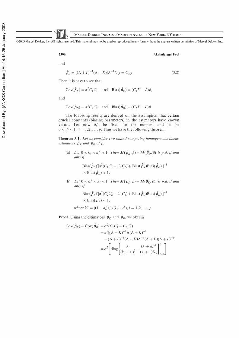
^D ¼ ½ð þ I Þ 1ð þ DÞ 1X 0 y ¼ C 2 y: ð3:2Þ

Then it is easy to see that

Cov ð ^K Þ ¼ 2C 1C 01 and Bias ð ^

K Þ ¼ ðC 1X I Þ ,

and

Cov ð ^D Þ ¼ 2C 2C 02 and Bias ð ^

D Þ ¼ ðC 2X I Þ :

The following results are derived on the assumption that certaincrucial constants (biasing parameters) in the estimators have knownvalues. Let now d i ’s be xed for the moment and let be0 < d i < 1, i ¼ 1,2, . . . , p. Thus we have the following theorem.

Theorem 3.1. Let us consider two biased competing homogeneous linearestimators ^

K and ^D of .

(a) Let 0 < k i < k i < 1. Then M ð ^K , Þ M ð ^

D , Þ is p.d. if and only if

Bias ð ^D Þ0½ 2ðC 1C 01 C 2C 02Þ þ Bias ð ^

K ÞBias ð ^K Þ

0 1

Bias ð ^D Þ < 1:

(b) Let 0 < k i < k i < 1. Then M ð ^D , Þ M ð ^

K , Þ, is p.d. if and only if

Bias ð ^K Þ

0½ 2ðC 2C 02 C 1C 01Þ þ Bias ð ^D ÞBias ð ^

D Þ0 1

Bias ð ^K Þ < 1,

where k i ¼ ðð1 d i Þ i Þ=ð i þ d i Þ, i ¼ 1,2, . . . , p.

Proof. Using the estimators ^K and ^

D , we obtain

Cov ð ^K Þ Cov ð ^

D Þ ¼ 2ðC 1C 01 C 2C 02Þ

¼ 2½ð þ K Þ 1 ð þ K Þ 1

ð þ I Þ 1ð þ DÞ 1ð þ DÞð þ I Þ 1

¼ 2 diag i

ðk i þ i Þ2

ð i þ d i Þ2

ð i þ 1Þ2i ( ) p

i ¼1" #






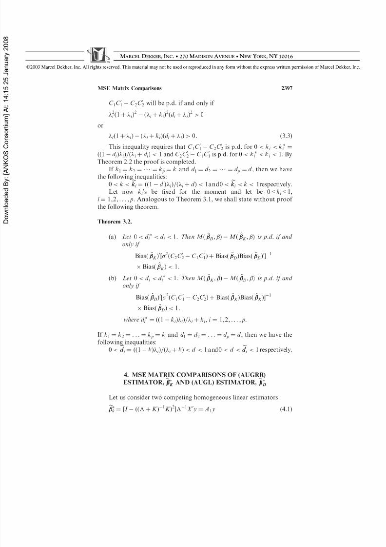
C 1C 01 C 2C 02 will be p.d. if and only if 2i ð1 þ i Þ

2 ð i þ ki Þ2ðd i þ i Þ

2 > 0

or

i ð1 þ i Þ ð i þ ki Þðd i þ i Þ > 0: ð3:3Þ

This inequality requires that C 1C 01 C 2C 02 is p.d. for 0 < k i < k i ¼ðð1 d i Þ i Þ=ð i þ d i Þ < 1 and C 2C 02 C 1C 01 is p.d. for 0 < k i < k i < 1. ByTheorem 2.2 the proof is completed.

If k1 ¼ k2 ¼ ¼ k p ¼ k and d 1 ¼ d 2 ¼ ¼ d p ¼ d , then we havethe following inequalities:

0 < k <

ekk i ¼ ðð1 d Þ i Þ=ð i þ d Þ < 1and0 <

ekk i < k < 1respectively.

Let now ki ’s be xed for the moment and let be 0< k i <1,i ¼ 1,2, . . . , p. Analogous to Theorem 3.1, we shall state without proof the following theorem.

Theorem 3.2.

(a) Let 0 < d i < d i < 1. Then M ð ^D , Þ M ð ^

K , Þ is p.d. if and only if

Bias ð ^K Þ

0½ 2ðC 2C 02 C 1C 01Þ þ Bias ð ^D ÞBias ð ^

D Þ0 1

Bias ð ^K Þ < 1:

(b) Let 0 < d i < d i < 1. Then M ð ^K , Þ M ð ^

D , Þ is p.d. if and

only if Bias ð ^

D Þ0½ 2ðC 1C 01 C 2C 02Þ þ Bias ð ^K ÞBias ð ^

K Þ1

Bias ð ^D Þ < 1:

where d i ¼ ðð1 ki Þ i Þ= i þ ki , i ¼ 1,2, . . . , p.

If k1 ¼ k2 ¼ . . . ¼ k p ¼ k and d 1 ¼ d 2 ¼ . . . ¼ d p ¼ d , then we have thefollowing inequalities:

0 < ed d i ¼ ðð1 kÞ i Þ=ð i þ kÞ < d < 1 and0 < d < ed d i < 1 respectively.

4. MSE MATRIX COMPARISONS OF (AUGRR)

ESTIMATOR, ebbK AND (AUGL) ESTIMATOR,

ebb D

Let us consider two competing homogeneous linear estimators

ek ¼ ½I ðð þ K Þ 1K Þ2 1X 0 y ¼ A 1 y ð4:1Þ






and

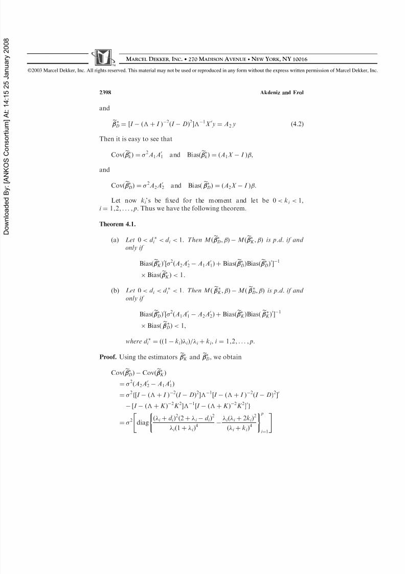
eD ¼ ½I ð þ I Þ 2ðI DÞ2 1X 0 y ¼ A 2 y ð4:2Þ

Then it is easy to see that

Cov ðekÞ ¼ 2A1A01 and Bias ðekÞ ¼ ðA1X I Þ ,

and

Cov ð

eD Þ ¼ 2A2A0

2 and Bias ð

eD Þ ¼ ðA2X I Þ :

Let now ki ’s be xed for the moment and let be 0 < k i < 1,i ¼ 1,2, . . . , p. Thus we have the following theorem.

Theorem 4.1.

(a) Let 0 < d i < d i < 1. Then M ðeD , Þ M ðeK , Þ is p.d. if and only if

Bias ðeK Þ0½ 2ðA2A0

2 A1A01Þ þ Bias ðeD ÞBias ðeD Þ0 1

Bias ðeK Þ < 1:

(b) Let 0 < d i < d i < 1. Then M ð

eK , Þ M ð

eD , Þ is p.d. if and

only if

Bias ðeD Þ0½ 2ðA1A01 A2A0

2Þ þ Bias ðeK ÞBias ðeK Þ0 1

Bias ðeD Þ < 1,

where d i ¼ ðð1 ki Þ i Þ= i þ ki , i ¼ 1,2, . . . , p.

Proof. Using the estimators eK and eD , we obtain

Cov ðeD Þ Cov ðeK Þ

¼ 2ðA2A02 A1A0

1Þ

¼ 2f½I ð þ I Þ 2ðI DÞ2 1½I ð þ I Þ 2ðI DÞ2 0

½I ð þ K Þ 2K 2 1½I ð þ K Þ 2K 2 0g

¼ 2 diag ð i þ d i Þ

2ð2 þ i d i Þ2

i ð1 þ i Þ4

i ð i þ 2k i Þ2

ð i þ ki Þ4( ) p

i ¼1" #






A2A02 A1A0

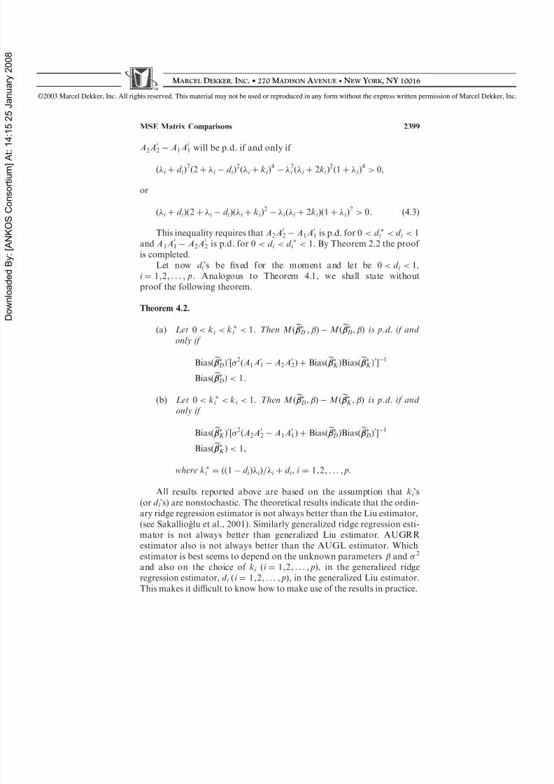
1 will be p.d. if and only if

ð i þ d i Þ2ð2 þ i d i Þ

2ð i þ ki Þ4 2

i ð i þ 2k i Þ2ð1 þ i Þ

4 > 0,

or

ð i þ d i Þð2 þ i d i Þð i þ ki Þ2 i ð i þ 2k i Þð1 þ i Þ

2 > 0: ð4:3Þ

This inequality requires that A2A02 A1A0

1 is p.d. for 0 < d i < d i < 1and A 1A0

1 A2A02 is p.d. for 0 < d i < d i < 1. By Theorem 2.2 the proof

is completed.Let now d i ’s be xed for the moment and let be 0 < d i < 1,

i ¼ 1,2, . . . , p. Analogous to Theorem 4.1, we shall state withoutproof the following theorem.

Theorem 4.2.

(a) Let 0 < k i < k i < 1. Then M ðeD , Þ M ðeD , Þ is p.d. if and only if

Bias ðeD Þ0½ 2ðA1A01 A2A0

2Þ þ Bias ðeK ÞBias ðeK Þ0 1

Bias ðeD Þ < 1:

(b) Let 0 < k i < k i < 1. Then M ð

eD , Þ M ð

eK , Þ is p.d. if and

only if

Bias ðeK Þ0½ 2ðA2A0

2 A1A01Þ þ Bias ðeD ÞBias ðeD Þ0 1

Bias ðeK Þ < 1,

where k i ¼ ðð1 d i Þ i Þ= i þ d i , i ¼ 1,2, . . . , p.

All results reported above are based on the assumption that ki ’s(or d i ’s) are nonstochastic. The theoretical results indicate that the ordin-ary ridge regression estimator is not always better than the Liu estimator,(see Sakalliog lu et al., 2001). Similarly generalized ridge regression esti-mator is not always better than generalized Liu estimator. AUGRR

estimator also is not always better than the AUGL estimator. Whichestimator is best seems to depend on the unknown parameters and 2

and also on the choice of ki ði ¼ 1,2, . . . , pÞ, in the generalized ridgeregression estimator, d i ði ¼ 1,2, . . . , pÞ, in the generalized Liu estimator.This makes it difficult to know how to make use of the results in practice.






For practical purposes, we have to replace these unknown parameters bysome suitable estimates.

5. SELECTION OF THE BIASING PARAMETERS ANDTHE OPERATIONAL ESTIMATORS

A very important issue in the study of ridge regression is how to ndappropriate parameters k i ði ¼ 1,2, . . . , pÞ. The nonnegative elements, k i ,are often referred to as biasing constants which may either benonstochastic or may depend on the observed data. The choice of values

for these biasing constants has been one of the most difficult problemsconfronting the study of the generalized ridge regression. However, whenk is data dependent, Monte Carlo studies are required for a moredenitive comparison of the two estimators as well as the determinationof the best rule for selecting k , (see McDonald and Galarneau, 1975).

Optimal values for the k i ’s in Eq. (2.6) can be considered to be thosek i ’s that minimize

Q 1 ¼ E ½ð ^K Þ0ð ^

K Þ :

With a certain amount of algebra, Q 1 may be expressed as

Q 1 ¼

X p

i ¼1

ð 2 i þ 2i k

2i Þ

ð i þ ki Þ2 :

Hoerl and Kennard (1970a, 1970b) have shown that the values of k i

which minimize the mean square error of ^K are given by

k i ðopt Þ ¼ 2

2i

, i ¼ 1,2, . . . , p: ð5:1Þ

Moreover, Hocking et al., (1976) showed that when these optimal k i

values in Eq. (5.1) are known, the generalized ridge regression estimatoris superior to all estimators within the class of biased estimators theyconsidered. Because these values are unknown, Hoerl and Kennard(1970a, 1970b) propose replacing the unknown quantities 2 and i by

their OLS estimates:

kk i ¼ 2

^2i

: ð5:2Þ






Hoerl et al., (1975) proposed the use of the harmonic mean of the k i

values; the arithmetic average will not be a good choice because verysmall i that have no predicting power would generate a very large kresulting in too much bias. The harmonic mean kh is calculated usingthe following formula:

kh ¼ 1

1= pP pi ¼1 1=k i

¼ p 2

0 :

Unfortunately, this interval for k is of limited practical value since itsupper bound depends on the true values of the parameters beingestimated. A widely used practice is to set

kkh ¼ kkHKB ¼ p 2

^0 ^: ð5:3Þ

However, in the presence of multicollinearity, ^0 is likely to be largeleading to the use of a very small k value. It is shown thatE ð 0 ^Þ ¼ 0 þ 2trace ðX 0X Þ 1. Thus, ^0 ^ is larger than 0 and thepoorer the conditioning of X 0X the larger the difference between ^0 ^

and 0 . The squared length of the ridge regression estimator based onkkHKB ¼ p 2 = ^00 ^, i.e., ~ ð kkHKB Þ, is going to be smaller than 0 ^. It seemsreasonable to expect an improvement if the ^ in kkHKB replaced by

~ ð kkHKB Þ. As k increases we know that ~ 0 ~ , the squared length of the ridge estimator, decreases.

Lawless and Wang estimates are given by

kkLW ¼ p

P pi ¼1 i =

kk i

¼ p 2

P pi ¼1 i

2i

ð5:4Þ

(see Lawless and Wang, 1976). Because the optimal kLW depends uponthe unknown quantities, an adaptive optimal k is instead obtained.Hemmerle and Brantle estimates are given by

kkðHB Þi ¼

i 2

i ^2

i 2if ei ð0Þ < 1

¼ 1 if ei ð0Þ 1

8>><>>:

ð5:5Þ

where

ei ð0Þ ¼ 2

i ^2

i






(see Hemmerle and Brantle, 1978). Troskie and Chalton estimates aregiven by

kkðTC Þi ¼

i 2

i ^2

i þ 2ð5:6Þ

(see Troskie and Chalton, 1996). Firinguetti (1999) proposed a newestimate of the optimal shrinkage parameters, k i ¼ 2= 2

i , namely:

kkðF Þi ¼

i 2

ðn pÞ 2 þ i 2

i

: ð5:7Þ

Replacing k i in K by kk i to form K K and substituting it in place of K inEq. (2.6) leads to an adaptive estimator of :

^ K K ¼ ð þ K K Þ 1X 0 y: ð5:8Þ

Optimal values for the d i ’s in Eq. (2.9) can be considered to be thosed i ’s that minimize

Q 2 ¼ E ½ð ^D Þ0ð ^

D Þ :

With a certain amount of algebra, Q 2 may be expressed as

Q 2 ¼ X p

i ¼1

ð 2ð i þ d i Þ2 þ i ð1 d i Þ

2 2i Þ

i ð i þ 1Þ2 : ð5:9Þ

Q2 is minimized at

d i ðopt Þ ¼ i ð

2i 2Þ

i 2i þ 2

: ð5:10Þ

Substituting d i (opt) in place of d i ði ¼ 1,2, . . . , pÞ in ^D provides an

‘‘estimator’’ which is useless for the simple reason that 2 and i areunknown. Thus, substituting 2 and i by their unbiased estimates 2

and ^i we obtain the estimate of d i :

^d d i ðOLS Þ ¼

i ð ^2i 2Þ

i ^2

i þ 2¼ 1

ð1 þ i Þ 2

i 2

i þ 2: ð5:11Þ

Unfortunately, we do not have any guarantee that these values arealways positive or between 0 and 1. We call this estimator the OLS-based






minimum mean square error estimator for d i (opt) . Thus we get a feasibleversion of the Liu stimator.

Now, consider the mean square error matrix of eK as,

M ðeK , Þ ¼ ½I U 2 1½I U 2 0 þ U 2 0U 02 ð5:12Þ

where U ¼ ð þ K Þ 1K . Considering only the i th diagonal element of Eq.(5.12) as, M i ðeK , Þ we have

M i ðeK , Þ ¼ 2 ð1 u2

i Þ2

i þ u4

i 2i ð5:13a Þ

and ordinary mean square error (mse) of

eK is

mse ðeK Þ ¼ tr ðM ðeD , ÞÞ ¼X p

i ¼1

ð1 u2i Þ

2 2

i þ X

p

i ¼1

u4i

2i ð5:13b Þ

where ui ¼ k i =ð i þ ki Þ. Nomura (1988) has shown that the optimal valueof k i for which the M i ðeK , Þ is minimum is

k i ðopt Þ ¼ 2 þ ffiffiffiffiffiffiffiffiffiffii

2i þ 2p 2

i : ð5:14Þ

If the individual k i in Eq. (5.14) are combined in some way to obtaina single value of k , Nomura (1988) suggested that a reasonable choice is

~ kkN ¼ p ^ 2

pi ¼1 ð 2

i Þ= 1 þ ffiffiffiffiffiffiffiffiffi1 þ i ð ^2

i = ^ 2Þq :

Similarly, we write the MSE matrix of eD from Eq. (2.9) as

M ðeD , Þ ¼ 2ðI 2Þ 1ðI 2Þ0 þ 2 0 02 ð5:15Þ

where ¼ ð þ I Þ 1ðI DÞ. Let us consider the i th term of M ðeD , Þ i.e.,

M i ð

eD , Þ ¼ ð1 2

i Þ2 2

i þ 4

i 2i ð5:16a Þ

and ordinary mean square error of eD is

mse ðeD Þ ¼ tr ðM ðeD , ÞÞ ¼X p

i ¼1

ð1 2i Þ

2 2

i þ X

p

i ¼1

4i

2i ð5:16b Þ






where i ¼ ð1 d i Þ=ð1 þ i Þ. Akdeniz et al., (1999) have shown that theoptimal choice of the parameter d i for which the M i ðeD , Þ is minimum is

d i ðopt Þ ¼ 1 ffiffiffiffiffiffiffiffiffiffi 2ð1 þ i Þ2

2 þ i 2i s : ð5:17Þ

Substituting the OLS estimators for 2 and i ’s in Eqs. (5.14) and(5.17), we obtain operational biasing parameters of the almost unbiasedgeneralized ridge regression estimator and the almost unbiased general-ized Liu estimator respectively.

6. NUMERICAL EXAMPLE

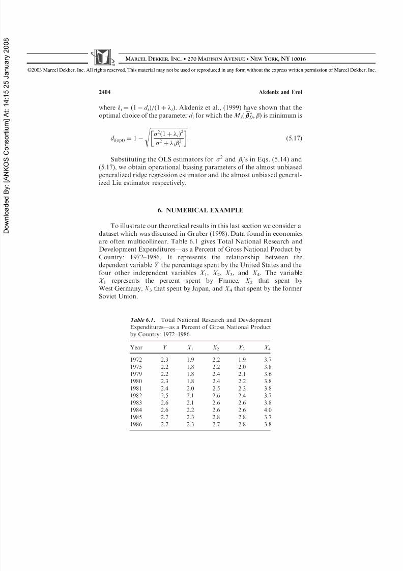
To illustrate our theoretical results in this last section we consider adataset which was discussed in Gruber (1998). Data found in economicsare often multicollinear. Table 6.1 gives Total National Research andDevelopment Expenditures—as a Percent of Gross National Product byCountry: 1972–1986. It represents the relationship between thedependent variable Y the percentage spent by the United States and thefour other independent variables X 1, X 2, X 3, and X 4. The variableX 1 represents the percent spent by France, X 2 that spent byWest Germany, X 3 that spent by Japan, and X 4 that spent by the formerSoviet Union.

Table 6.1. Total National Research and DevelopmentExpenditures—as a Percent of Gross National Productby Country: 1972–1986.

Year Y X 1 X 2 X 3 X 4

1972 2.3 1.9 2.2 1.9 3.71975 2.2 1.8 2.2 2.0 3.81979 2.2 1.8 2.4 2.1 3.61980 2.3 1.8 2.4 2.2 3.81981 2.4 2.0 2.5 2.3 3.81982 2.5 2.1 2.6 2.4 3.71983 2.6 2.1 2.6 2.6 3.81984 2.6 2.2 2.6 2.6 4.01985 2.7 2.3 2.8 2.8 3.71986 2.7 2.3 2.7 2.8 3.8






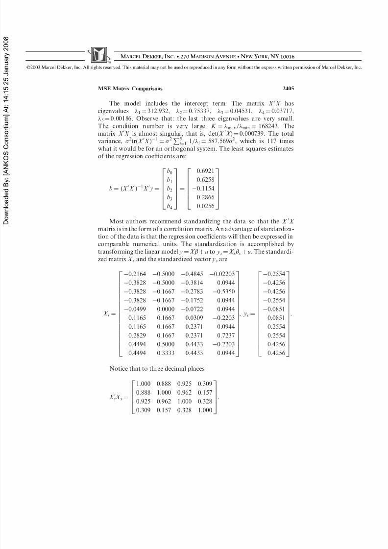
The model includes the intercept term. The matrix X 0X haseigenvalues 1 ¼ 312.932, 2 ¼ 0.75337, 3 ¼ 0.04531, 4 ¼ 0.03717,

5 ¼ 0.00186. Observe that: the last three eigenvalues are very small.The condition number is very large. K ¼ max = min ¼ 168243. Thematrix X 0X is almost singular, that is, det( X 0X ) ¼ 0.000739. The totalvariance, 2tr ðX 0X Þ 1 ¼ 2P5

i ¼1 1= i ¼ 587 :569 2, which is 117 timeswhat it would be for an orthogonal system. The least squares estimatesof the regression coefficients are:

b ¼ ðX 0X Þ 1X 0 y ¼

b0

b1

b2

b3

b4

2666664

3777775

¼

0:69210:62580:11540:28660:0256

2666664

3777775

Most authors recommend standardizing the data so that the X 0X matrix is in the form of a correlation matrix. An advantage of standardiza-tion of the data is that the regression coefficients will then be expressed incomparable numerical units. The standardization is accomplished bytransforming the linear model y ¼ X þ u to ys ¼ X s s þ u. The standardi-zed matrix X s and the standardized vector ys are

X s ¼

0:2164 0:5000 0:4845 0:022030:3828 0:5000 0:3814 0 :09440:3828 0:1667 0:2783 0:53500:3828 0:1667 0:1752 0 :09440:0499 0 :0000 0:0722 0 :09440:1165 0 :1667 0 :0309 0:22030:1165 0 :1667 0 :2371 0 :09440:2829 0 :1667 0 :2371 0 :72370:4494 0 :5000 0 :4433 0:22030:4494 0 :3333 0 :4433 0 :0944

2666666666666666664

3777777777777777775

, ys ¼

0:25540:42560:42560:25540:08510:08510:25540:25540:42560:4256

2666666666666666664

3777777777777777775

:

Notice that to three decimal places

X 0sX s ¼

1:000 0 :888 0 :925 0 :3090:888 1 :000 0 :962 0 :1570:925 0 :962 1 :000 0 :3280:309 0 :157 0 :328 1 :00026664 37775

:






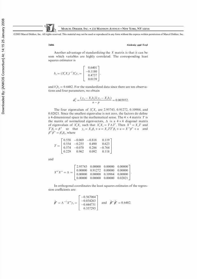
Another advantage of standardizing the X matrix is that it can beseen which variables are highly correlated. The corresponding leastsquares estimator is

bs ¼ ðX 0sX sÞ1X 0s ys ¼

0:64010:11800:47370:0139

26643775

:

and b0sbs ¼ 0:6482. For the standardized data since there are ten observa-

tions and four parameters, we obtain

^ 2s ¼ ð ys X sbsÞ0ð ys X sbsÞn p

¼ 0:003932 :

The four eigenvalues of X 0sX s are 2.95743, 0.91272, 0.10984, and0.02021. Since the smallest eigenvalue is not zero, the factors do denea 4-dimensional space in the mathematical sense. The 4 4 matrix T isthe matrix of normalized eigenvectors, i s a 4 4 diagonal matrixof eigenvalues of X 0sX s such that X 0sX s ¼ T T 0. Then X ¼ X sT andT 0 s ¼ so that ys ¼ X s s þ u ¼ X sTT 0

s þ u ¼ X þ u and0 ¼ 0

s s , where

T ¼

0:558 0:069 0:818 0 :1190:554 0:255 0 :490 0 :6230:574 0:070 0 :286 0:7640:229 0 :962 0 :092 0 :1182664 3775

and

X 0X ¼ ¼

2:95743 0 :00000 0 :00000 0 :000000:00000 0 :91272 0 :00000 0 :000000:00000 0 :00000 0 :10984 0 :000000:00000 0 :00000 0 :00000 0 :02021

26643775

:

In orthogonal coordinates the least squares estimates of the regres-sion coefficients are:

^ ¼ 1X 0 ys ¼

0:5670640:0342630:4447310:357295

2664 3775 and ^ 0 ^ ¼ 0:6482 :






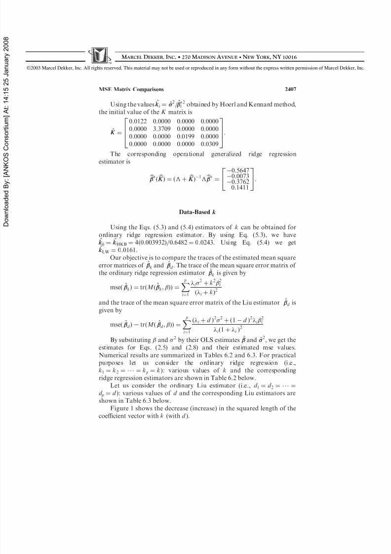
Using the values kk i ¼ 2=^ 2i obtained by Hoerl and Kennard method,

the initial value of the K matrix is

K K ¼

0:0122 0 :0000 0 :0000 0 :00000:0000 3 :3709 0 :0000 0 :00000:0000 0 :0000 0 :0199 0 :00000:0000 0 :0000 0 :0000 0 :0309

26643775

:

The corresponding operational generalized ridge regressionestimator is

bð

bK K Þ ¼ ð þ

bK K Þ 1

b¼

0:56470:00730:37620:1411

24

35

:

Data-Based k

Using the Eqs. (5.3) and (5.4) estimators of k can be obtained forordinary ridge regression estimator. By using Eq. (5.3), we havekkh ¼ kkHKB ¼ 4ð0:003932 Þ=0:6482 ¼ 0:0243. Using Eq. (5.4) we getkkLW ¼ 0:0161.

Our objective is to compare the traces of the estimated mean squareerror matrices of ^

k and ^d . The trace of the mean square error matrix of

the ordinary ridge regression estimator ^k is given by

mse ð ^

kÞ ¼ tr ðM ð ^

k, ÞÞ ¼

X p

i ¼1

i 2 þ k2 2i

ð i þ kÞ2

and the trace of the mean square error matrix of the Liu estimator ^d is

given by

mse ð ^d Þ ¼ tr ðM ð ^

d , ÞÞ ¼X p

i ¼1

ð i þ d Þ2 2 þ ð 1 d Þ2i

2i

i ð1 þ i Þ2

By substituting and 2 by their OLS estimates ^ and 2, we get theestimates for Eqs. (2.5) and (2.8) and their estimated mse values.Numerical results are summarized in Tables 6.2 and 6.3. For practicalpurposes let us consider the ordinary ridge regression (i.e.,k1 ¼ k2 ¼ ¼ k p ¼ k): various values of k and the correspondingridge regression estimators are shown in Table 6.2 below.

Let us consider the ordinary Liu estimator (i.e., d 1 ¼ d 2 ¼ ¼d p ¼ d ): various values of d and the corresponding Liu estimators areshown in Table 6.3 below.

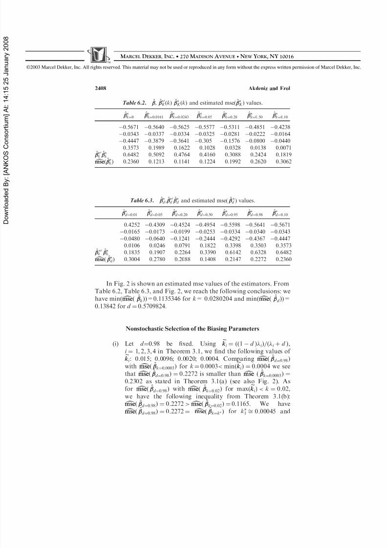
Figure 1 shows the decrease (increase) in the squared length of thecoefficient vector with k (with d ).






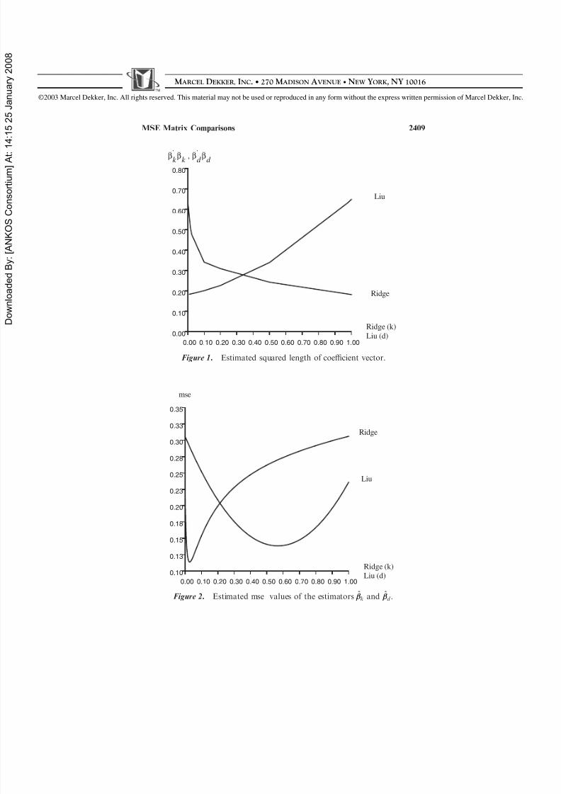
In Fig. 2 is shown an estimated mse values of the estimators. FromTable 6.2, Table 6.3, and Fig. 2, we reach the following conclusions: wehave min( dmsemse( ^

k ))=0.1135346 for k= 0.0280204 and min( dmsemse( ^d ))=

0.13842 for d ¼ 0.5709824.

Nonstochastic Selection of the Biasing Parameters

(i) Let d ¼0.98 be xed. Using ekk i ¼ ðð1 d Þ i Þ=ð i þ d Þ,i ¼ 1, 2, 3, 4 in Theorem 3.1, we nd the following values of

ekk i : 0.015; 0.0096; 0.0020; 0.0004. Comparing dmsemse ð ^d ¼0:98Þ

with

dmsemse ð ^

k¼0:0003 Þ for k ¼ 0.0003 < min ð

ekk i Þ ¼ 0:0004 we see

that

dmsemse ð ^

d ¼0:98Þ ¼ 0:2272 is smaller than

dmsemse ð ^

k¼0:0003 Þ ¼

0:2302 as stated in Theorem 3.1(a) (see also Fig. 2). Asfor dmsemse( ^d ¼0:98 ) with dmsemse( ^

k¼0:02 ) for max ðekk i Þ < k ¼ 0:02,we have the following inequality from Theorem 3.1(b):

dmsemse ð ^d ¼0:98Þ ¼ 0:2272 > dmsemse ð ^

k¼0:02 Þ ¼0:1165. We have

dmsemse ð ^d ¼0:98Þ ¼ 0:2272 ¼ dmsemse ð ^

k¼k Þ for k1 ffi 0:00045 and

Table 6.2. , ^ 0K ðkÞ ^

K ðkÞ and estimated mse ð ^K Þ values.

^k¼0

^k¼0:0161

^k¼0:0243

^k¼0:05

^k¼0:20

^k¼0:50

^k¼0:10

0.5671 0.5640 0.5625 0.5577 0.5311 0.4851 0.42380.0343 0.0337 0.0334 0.0325 0.0281 0.0222 0.01640.4447 0.3879 0.3641 0.305 0.1576 0.0800 0.04400.3573 0.1989 0.1622 0.1028 0.0328 0.0138 0.0071

^ 0k

^k 0.6482 0.5092 0.4764 0.4160 0.3088 0.2424 0.1819

dmsemse ð ^kÞ 0.2360 0.1213 0.1141 0.1224 0.1992 0.2620 0.3062

Table 6.3. ^d , ^ 0

d ^

d and estimated mse ð ^d Þ values.

^d ¼0:01

^d ¼0:05

^d ¼0:20

^d ¼0:50

^d ¼0:95

^d ¼0:98

^d ¼0:10

0.4252 0.4309 0.4524 0.4954 0.5598 0.5641 0.56710.0165 0.0173 0.0199 0.0253 0.0334 0.0340 0.03430.0480 0.0640 0.1241 0.2444 0.4292 0.4367 0.44470.0106 0.0246 0.0791 0.1822 0.3398 0.3503 0.3573

^ 0k

^k 0.1835 0.1907 0.2264 0.3390 0.6142 0.6328 0.6482

dmsemse ð ^d Þ 0.3004 0.2780 0.2088 0.1408 0.2147 0.2272 0.2360






Ridge (k)Liu (d)

Ridge

Liu

d d k k ββββ ˆ'ˆ

,ˆ'ˆ

0.10 0.30 0.50 0.70 0.900.00 0.20 0.40 0.60 0.80 1.00

0.10

0.30

0.50

0.70

0.00

0.20

0.40

0.60

0.80

Figure 1. Estimated squared length of coefficient vector.

Ridge (k)Liu (d)

Liu

Ridge

mse

0.10 0.30 0.50 0.70 0.900.00 0.20 0.40 0.60 0.80 1.00

0.13

0.18

0.23

0.28

0.33

0.10

0.15

0.20

0.25

0.30

0.35

Figure 2. Estimated mse values of the estimators ^k and ^

d .






k2 ffi 0:2977973, then dmsemse ð ^d ¼0:98Þ > dmsemse ð ^

kÞ for ðmax ðekk i Þ <k < k2Þ.

(ii) Let k¼0.02 be xed. Using ed d i ¼ ðð1 kÞ i Þ= i þ k, i ¼ 1, 2, 3, 4in Theorem 3.2, we nd the following values of ed d i : 0.9734;0.9590; 0.8290; 0.4924. In this case dmsemse ð ^

kÞ ¼ 0:1165 <

dmsemse ð ^d Þ ¼ 0:2272 for 0 < max ðed d i ¼ 0:9734 Þ < d ¼ 0:98 as

stated in Theorem 3.2 (a). Since the condition in Theorem 3.2(b) does not hold, dmsemse ð ^

d ¼0:40Þ ¼ 0:1530 is not smaller than

dmsemse ð ^k¼0:02Þ ¼ 0:1165 for 0 < d ¼ 0:40 < min ðed d i ¼ 0:4924).

(iii) k ¼ 0.20 be xed. We nd ed d i ¼ ðð1 0:20Þ i Þ= i þ 0:20: 0.7493;0.6562; 0.2836; 0.0734 using Theorem 3.2.

dmsemse ð ^

k¼0:20Þ ¼0:1992 and

dmsemse ð ^

d ¼0:80Þ ¼ 0:1666 for d ¼ 0:80 > max ð

ed d i Þ ¼

0:7493. Since the condition in Theorem 3.2 (a) does not hold,

dmsemse ð ^k¼0:20Þ is not smaller than dmsemse ð ^

d ¼0:80Þ. We have

dmsemse ð ^k¼0:20Þ ¼ 0:1992 and dmsemse ð ^

d ¼0:05 Þ ¼ 0:2780 for d ¼0:05 < min ðed d i Þ ¼ 0:0734. Since the condition in Theorem 3.2(b) does not hold, dmsemse ð ^

k¼0:20Þ dmsemse ð ^d ¼0:05Þ is not positive.

But we have dmsemse ð ^k¼0:20Þ ¼ 0:1992 ¼ dmsemse ð ^

d ¼d Þ for d 1 ffi0:2259032 and d 2 ffi 0:9088346. Then dmsemse ð ^

d < d 1Þ

dmsemse ð ^k¼0:20Þ and dmsemse ð ^

d > d 2Þ dmsemse ð ^

k¼0:20Þ is positive.

0.10 0.30 0.50 0.70 0.900.00 0.20 0.40 0.60 0.80 1.00

0.13

0.18

0.23

0.28

0.33

0.10

0.15

0.20

0.25

0.30

0.35

Ridge (k)Liu (d)

AULiu

AURidge

mse

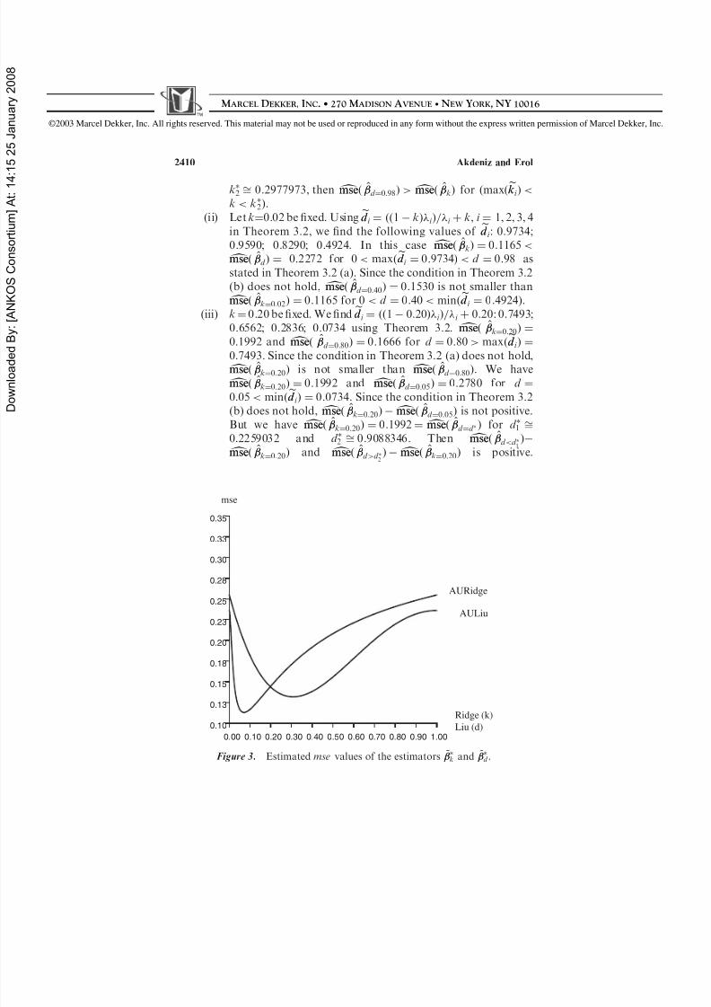
Figure 3. Estimated mse values of the estimators ~ k and ~

d .






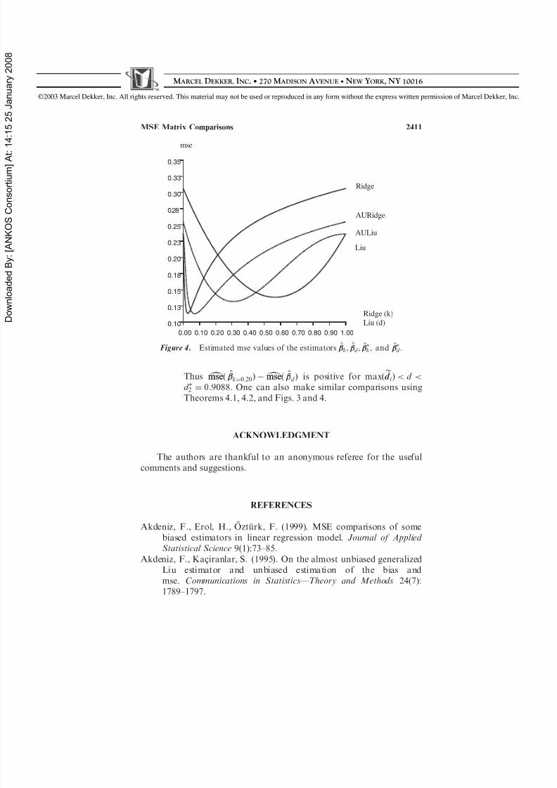
Thus dmsemse ð ^k¼0:20Þ dmsemse ð ^

d Þ is positive for max ðed d i Þ < d <d 2 ¼ 0:9088. One can also make similar comparisons usingTheorems 4.1, 4.2, and Figs. 3 and 4.

ACKNOWLEDGMENT

The authors are thankful to an anonymous referee for the usefulcomments and suggestions.

REFERENCES

Akdeniz, F., Erol, H., O ztu rk, F. (1999). MSE comparisons of somebiased estimators in linear regression model. Journal of Applied

Statistical Science 9(1):73–85.Akdeniz, F., Kac iranlar, S. (1995). On the almost unbiased generalizedLiu estimator and unbiased estimation of the bias andmse. Communications in Statistics—Theory and Methods 24(7):1789–1797.

Ridge (k)Liu (d)

AULiu

Ridge

mse

AURidge

Liu

0.10 0.30 0.50 0.70 0.900.00 0.20 0.40 0.60 0.80 1.00

0.13

0.18

0.23

0.28

0.33

0.10

0.15

0.20

0.25

0.30

0.35

Figure 4. Estimated mse values of the estimators ^k , ^

d , ~ k , and ~

d .






Farebrother, R. W. (1976). Further results on the mean square errorof ridge regression. Journal of the Royal Statistical Society B.38:248–250.

Firinguetti, L. (1999). A generalized ridge regression estimator and itsnite sample properties. Communications in Statistics—Theory and Methods 28(5):1217–1229.

Gnot, S., Trenkler, G., Zmyslony, R. (1995). Non-negative minimumbiased quadratic estimation in the linear regression models.Journal of Multivariate Analysis 4(1):113–125.

Gruber, M. H. J. (1998). Improving Efficiency by Shrinkage : The JamesStein and Ridge Regression Estimators . New York: Marcel Dekker.

Hemmerle, W. J., Brantle, T. F. (1978). An explicit and constrainedgeneralized ridge estimation. Technometrics 20:109–119.

Hocking, R. R., Speed, F. M., Lynn, M. J. (1976). A class of biasedestimators in linear regression. Technometrics 18:425–437.

Hoerl, A. E., Kennard, R. (1970a). Ridge regression: biased estimationfor non-orthogonal problems. Technometrics 12:55–67.

Hoerl, A. E., Kennard, R. W. (1970b). Ridge regression: application fornon-orthogonal problems. Technometrics 12:69–82.

Hoerl, A. E., Kennard, R., Baldwin, K. F. (1975). Ridge regression: somesimulations. Communications in Statistics—Theory and Methods4(2):105–123.

Kac iranlar, S., Sakalliog lu, S., Akdeniz, F., Styan, G. P. H., Werner, H. J.(1999). A new biased estimator in linear regression and a detailedanalysis of the widely-analyzed dataset on Portlandcement.Sankhya : The Indian Journal of Statistics 61(Series B):443–459.

Lawless, J. F., Wang, P. (1976). A simulation study of ridge and otherregression estimators. Communications in Statistics—Theory and Methods A5:307–323.

Liu, Ke Jian. (1993). A new class of biased estimate in linear regression.Communications in Statistics—Theory and Methods 22(2):393–402.

McDonald, G. C., Galarneau, D. I. (1975). A Monte Carlo evaluation of some ridge type estimators. Journal of the American Statistical Association 70:407–416.

Nomura, M. (1988). On the almost unbiased ridge regression estimator.Communications in Statistics — Simulation and Computation 17:729–743.

Rao, C. R., Toutenburg, H. (1995). Linear Models Least Squares and Alternatives . New York: Springer-Verlag.Sakalliog lu, S., Kac iranlar, S., Akdeniz, F. (2001). Mean squared error

comparisons of some biased regression estimators. Communicationsin Statistics—Theory and Methods 30(2):347–361.






Singh, B., Chaubey, Y. P., Dwivedi, T. D. (1986). An almost unbiasedridge estimator. Sankhya : The Indian Journal of Statistics 48(SeriesB):342–346 :

Stein, C. (1956). Inadmissibility of usual estimator for the mean of amulti-variate normal distribution. Proceedings of the Third Berkeley Symposium on Mathematical Statistics and Probability ,Berkeley: University of California Press, 197–206.

Theobald, C. M. (1974). Generalizations of mean square error appliedto ridge regression. Journal of the Royal Statistical SocietyB.36:103–106.

Trenkler, G., Toutenburg, H. (1990). Mean squared error matrixcomparisons between biased estimators an overview of recentresults. Statistical Papers 31:165–179.

Troskie, C. G., Chalton, D. O. (1996). A Bayesian estimate for theconstants in ridge regression. South African Statistical Journal 30:119–137.


akdeniz erol 2003

Documents