arX

iv:1

505.

0225

5v1

[m

ath.

CA

] 9

May

201

5

A hypergeometric treatment to explain the nonlinear true behavior of

redundant constraints on a straight elastic rod

Giovanni Mingari Scarpello ∗ Daniele Ritelli †

Abstract

In theory and practice of elastic straight rods, the statically indeterminate reactions acted by perfectconstraints are commonly believed not to depend on the flexural stiffness EJ . We solve exactly two elasticaproblems in order to obtain hypergeometrically (helped by Lagrange, Lauricella, Appell), the true displace-ments upon which the forces method is founded. As a consequence, the above reactions are found to dependon stiffness: the presumptive independence credited as general, is far from being always true, but, quite thecontrary, is valid only within a first-order approximation.

Keyword: Non-Linear Rod Theory, Statical Redundancy, Elliptic and Hypergeometric Integrals, LauricellaFunctions.

1 Introduction

In 1691, Jakob Bernoulli proposed to find out the deformed centerline (planar ”elastica”) of a thin, homogeneous,straight and flexible rod under a force applied at its end. He established, Curvatura laminae elasticae (1694),the differential equation of the centerline, say y = y(x), of the rod ab appenso pondere curvata to be:

dy =x2dx√1− x4

His nephew, Daniel Bernoulli, computed the potential energy stored in a bent rod and, in 1742, wrote to L.Euler that the rod should attain such a shape as to minimize the functional of squared curvature. Accordingly,Euler dealt elastica as an isoperimetric problem of Calculus of Variations, De curvis elasticis (1744), arriving atelastica’s differential equation and identifying nine shapes of the curve, all equilibrium states of minimal energy.

Anyway, C. Maclaurin had realized the elastica’s connection to elliptic integrals, see A treatise on fluxions

(1742), § 927 entitled: “The construction of the elastic curve, and of other figures, by the rectification of the

conic sections”. In 1757, Euler authored a paper, Sur la force des colonnes, concerning the buckling of columnsagain, where the critical load is approached through a simplified expression to the elastica’s curvature.

Some analytical solutions to elastic planar curves through elliptic integrals of the first and second kind,can be read at [17], [4] and [18]. Almost half a century ago, [7], collected many problems on the base of theconstraint type, and all solved by the elliptic integrals of first and second kind, while the third kind and Thetafunctions appear marginally for 3−D deformations. In order to set the record straight, the concept of rod willbe recalled from [8]:

A “rod” is something of a hybrid, i. e. a mathematical curve made up of “material points”. Ithas no cross section, yet it has stiffness. It can weigh nothing or it can be heavy. We can twistit, bend it, stretch it and shake it, but we cannot break it, it is completely elastic. Of course, itis a mathematical object, and does not exist in the physical world; yet it finds wide applicationin structural (and biological) mechanics: columns, struts, cables, thread, and DNA have all beenmodeled with rod theory.

In common practice, a simplified expression to the elastica’s curvature is currently used, while the real exactexpression leads to nonlinearities.

∗giovannimingari@yahoo.it†Dipartimento scienze statistiche, viale Filopanti, 5 40127 Bologna Italy, daniele.ritelli@unibo.it

1

The link between elliptic functions and elastica was always understood to be close, to induce the ellipticfunctions to be plotted through suitable curved rubber rods [9], while the paper [1] is founded on the use ofthe Weierstrass ℘ function. Even in contemporary literaure the touchs of the special functions with elasticaproblems are very close, [7]. In fact, the situations one can meet require either a numerical [19], or an ellipticapproach [5, 12, 13, 14] or a hypergeometric [15]. In this paper we will follow the last one.

2 Aim of the paper

There is a large amount of literature providing the true elastica by solving the relevant nonlinear deflectionequation (3.2), where the rod’s curvature is forced by a bending moment. As a matter of fact in [15], wesolved the nonlinear deflection problem, as a pure strain analysis, for slender rods by means of Lauricellahypergeometric functions.

Nevertheless, as far as we are concerned, the nonlinear, deflection analysis has never been used for a furtherstatic analysis until now.

We refer to statically indeterminate structures, of which the degree of redundancy is the excess of constraintsbeyond the strictly necessary. This terminology is currently used as one can see in the literature, see for instance[11], or the Wikipedia entry “Statically indeterminate”.

Such systems require additional equations and cannot be analyzed through the equilibrium equations alone.On the purpose, a frequent approach, the so–called forces method, obtains them by transforming the givenredundant structure into a so–called simple one, i.e. a statically determinate one, by replacing the redun-dant constraints with the unknown reactions. This will not introduce alterations in stress distribution and indeflections. By decoupling such a multiple load condition over the simple structure in each load stage, eachcorresponding displacement is computed as a function of the system parameters (say E, J, L, . . .) and the re-dundant unknowns. Finally, one shall require the consistency, namely that the displacement composition meetsthe real situation. And so we can have consistency to a zero displacement (perfect constraint), or to a certainimposed value (anelastic yield) or to a damper effect (elastic yield): in such a way the necessary elasticityequations are finally obtained. All the computing work one does about such deflections of straight rods of spanL is grounded upon the small strains assumption: if y(x) is the deformed centerline’s equation, for each x itshall be:

y2x ≪ 1 with 0 ≤ x ≤ L. (2.1)

In such a way, all further steps -and the statically indeterminate reactions- lose their validity when the loadintensity, beam slenderness, or high flexibility, causes the relevant strain-even kept in the linear elasticity (effectproportional to its cause) to be such that (2.1) becomes. In such cases, the exact centerline curvature is necessaryand the nonlinear ODE (3.1) of deflections is often employed in advanced applications regarding the strengthof materials in the contexts of aerospace or satellites, see [2].

We are just going, on the ground of these new considerations, to compute the statical indeterminate unknownsthrough a nonlinear deflection analysis.

3 Statement of the problem

Let us tackle a L-long, thin rod whose end is clamped and A free. We put at A the origin of a (x, y) cartesianreference frame with x along the undeformed rod, from the wall to A; and y downwards, normal at A to x, seeFigure 1. Our basic assumptions are:

A1 the rod is thin, initially straight, homogeneous, with a uniform cross section and uniform flexural stiffnessEJ , where E is the Young modulus, and J, the cross section moment of inertia about a “neutral” axisnormal to the plane of bending and passing through the central line;

A2 the slender rod is always charged by coplanar dead (not follower) loads;

A3 Linear constitutive load holds: so that the induced curvature is proportional via 1/(EJ) to the bendingmoment.

A4 The shear transverse deformation is ignored.

A5 A stationary strain field, by isostatic equilibrium of active loads and reactive forces takes place, and, dueto rest of static equilibrium, no rod element undergoes acceleration.

2

The key Bernoulli-Euler linear constitutive law connects flexural stiffness EJ and bending moment M tothe consequent curvature κ of the deflected centerline: ±EJκ = M (x). With our (traditional) reference frame(x, y), the curvature always bears the opposite sign to the bending moment:

EJyxx

(1 + y2x)3/2

= −M (x) (3.1)

where y = y(x) is the unknown elastica’s equation and

yx =dy

dx, yxx =

d2y

dx2.

To (3.1) a useful dress can be given, so that it shall be minded that the Cauchy problem:

d

dx

(

yx√

1 + y2x

)

= − 1

EJM (x), 0 ≤ x ≤ L

y(L) = 0

yx(L) = 0

(3.2)

can be solved in such a way. Putting:

H(x) :=

∫ L

x

M (ξ)dξ

the solution of (3.2) is:

y(x) = −∫ L

x

H(ξ)√

(EJ)2 −H2(ξ)

dξ. (3.3)

In order to have a solution defined for x ∈ [0, L] we have to require that

− 1 <1

EJH(x) < 1 (3.4)

which is a general prescription on the load effects and will be defined in single cases.

3.1 Nonlinear deflection, a first example

For a L, E, J cantilever tip-sheared by P , the approximate linear theory provides a tip’s vertical displacementδ0 = (PL3)/(3EJ). In such a case, in (3.2) we put M (x) = −Px and defining the nondimensional quantities:

µ =PL3

3EJ; η =

y

L; ξ =

x

L

it becomes δ0 = 2µ/3.Formula (2.32) of our previous paper [15] for the exact free-end displacement provides:

η(ξ) =µ

3 (1− µ2)3/2

ξ3 − µ√

1− µ2ξ +

√

µ

2A(µ)

where A(µ) is a complicated function involving elliptic integrals of first and third kind according to formula(2.29) of the same [15]. They can be expanded with respect to µ, with initial point µ0 = 0; then, recalling theMaclaurin first–order expansion with respect to µ

µ

3 (1− µ2)3/2

ξ3 − µ√

1− µ2ξ = µ

(

ξ3

3− ξ

)

+O(

µ2)

(3.5)

one obtains eventually

η(ξ) =µ

3

(

2− 3ξ + ξ3)

+O(

µ2)

(3.6)

i.e. the usual approximation which for ξ = 0 (free tip) provides the same deflection δ0 as above.

3

O

LP

x

y

‘A

δο

A

Δ

A

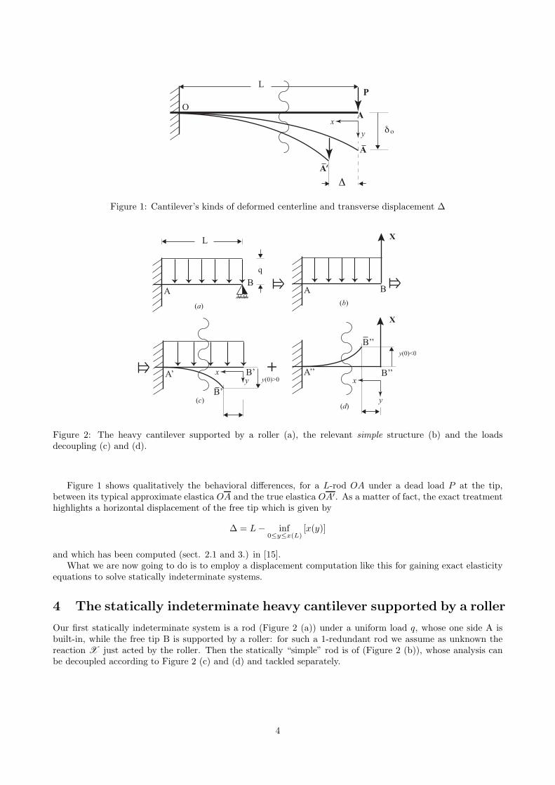
Figure 1: Cantilever’s kinds of deformed centerline and transverse displacement ∆

xy

A’ B’ A’’ B’’

X

(a) (b)

(c)

L

AB

q

A B

X

x

y

+

(d)

y(0)>0

y(0)<0

B’

B’’

Figure 2: The heavy cantilever supported by a roller (a), the relevant simple structure (b) and the loadsdecoupling (c) and (d).

Figure 1 shows qualitatively the behavioral differences, for a L-rod OA under a dead load P at the tip,between its typical approximate elastica OA and the true elastica OA′. As a matter of fact, the exact treatmenthighlights a horizontal displacement of the free tip which is given by

∆ = L− inf0≤y≤x(L)

[x(y)]

and which has been computed (sect. 2.1 and 3.) in [15].What we are now going to do is to employ a displacement computation like this for gaining exact elasticity

equations to solve statically indeterminate systems.

4 The statically indeterminate heavy cantilever supported by a roller

Our first statically indeterminate system is a rod (Figure 2 (a)) under a uniform load q, whose one side A isbuilt-in, while the free tip B is supported by a roller: for such a 1-redundant rod we assume as unknown thereaction X just acted by the roller. Then the statically “simple” rod is of (Figure 2 (b)), whose analysis canbe decoupled according to Figure 2 (c) and (d) and tackled separately.

4

4.1 First sub-system: the heavy cantilever

Let us consider first the subsystem of Figure 2 (c). For the bending moment we have M (x) = −(q/2)x2.Specializing (3.4) for this load, it will imply q < 6EJ/L3. Thus (3.3) reads1 as

y(x) =

∫ L

x

q(L3 − y3)

6

√

1−(

EJ6

)2(L3 − y3)2

dy =2EJ

qL2

∫q

6EJ(L3−x3)

0

u

(1− u2)1/2(

1− 6EJqL3 u

)2/3du (4.1)

Now using the Lauricella functions’ integral representation theorem, we infer the integration formula

∫ a

0

u

(1− u2)1/2(1− bu)2/3du =

a2

2F(3)D

(

2; 1/2, 1/2, 2/3

2

∣

∣

∣

∣

∣

a,−a, ab

)

(4.2)

Clearly (4.2) is the key to evaluate the integral in (4.1), so that

y(x) =q(

L3 − x3)2

36EJL2F(3)D

(

2; 1/2, 1/2, 2/3

3

∣

∣

∣

∣

∣

q

6EJ(L3 − x3),− q

6EJ(L3 − x3), 1 − x3

L3

)

(4.1b)

which provides the deflection law for each x. We are interested to take x = 0 in (4.1b) getting

y(0) =L4q

36EJF(3)D

(

2; 1/2, 1/2, 2/3

3

∣

∣

∣

∣

∣

L3q

6EJ,− L3q

6EJ, 1

)

(4.1c)

Notice that for x = 0 the third argument of Lauricella’s becomes 1, so that such a function collapses into anAppell one and from there it can be reduced to a 3F2 hypergeometric function, as shown in section 6. In sucha way we will be allowed to describe the strain by means of a function of only one variable. We can simplify(4.1c) using the reduction formulae (6.3) and (6.4) in sequence, getting

y(0) =L4q

8EJ3F2

(

12 , 1,

32

76 ,

53

∣

∣

∣

∣

∣

L6q2

36(EJ)2

)

(4.1d)

which provides as a function of q, L, E, J the free tip true deflection of rod of Figure 2 (c).

4.2 Second sub-system: the tip-sheared cantilever

Allow us consider the subsystem of Figure 2 (d). The bending moment being M (x) = X x, so that (3.3) readsas

y(x) =

∫ L

x

X (y2 − L2)√

(2EJ)2 − X 2(y2 − L2)2dy =

X

4EJL

∫ 0

x2−L2

u(

1−(

X

2ELu)2)1/2

(

1 + 1L2u

)1/2du (4.3)

With the integral representation theorem we also infer the integration formula

∫ a

0

u

(1− b2u2)1/2(1 + cu)1/2du =

a2

2F(3)D

(

2; 1/2, 1/2, 1/2

3

∣

∣

∣

∣

∣

ab,−ab,−ac

)

(4.4)

Clearly, (4.4) is the key to evaluate the integral in (4.3), giving

y(x) = −(

x2 − L2)2

X

8EJLF(3)D

(

2; 1/2, 1/2, 1/2

3

∣

∣

∣

∣

∣

(x2 − L2)X

2EJ,− (x2 − L2)X

2EJ, 1− x2

L2

)

(4.3b)

1The approach of computing the exact tip position of the rod would be extremely long and capable of hiding the sense of thisresearch deviating by its central purpose. In such a way the (very small) horizontal deflection of the tip has been put to zero.Anyway, an example where the rod is assumed inextensible and the axial deformation is kept in account, can be seen in our previouspaper [14] sect. 3, formula (3.12).

5

We are interested to take x = 0 in (4.3b), getting

y(0) = −L4X

8EJF(3)D

(

2; 1/2, 1/2, 1/2

3

∣

∣

∣

∣

∣

− L2X

2EJ,L2X

2EJ, 1

)

(4.3c)

We can simplify (4.3c) using the reduction formulae (6.3) and (6.4) in sequence, getting

y(0) = −L3X

3EJ3F2

(

12 , 1,

32

54 ,

74

∣

∣

∣

∣

∣

L4X 2

4(EJ)2

)

(4.3d)

4.3 Consistency

In order to evaluate the redundant unknown X , notice that the addition of two displacements given by (4.1d)and (4.3d) shall be zero, arriving at the transcendental equation:

3Lq 3F2

(

12 , 1,

32

76 ,

53

∣

∣

∣

∣

∣

L6q2

36(EJ)2

)

− 8X 3F2

(

12 , 1,

32

54 ,

74

∣

∣

∣

∣

∣

L4X 2

4(EJ)2

)

= 0 (4.5)

in our unknown reaction X . Of course, (4.5) cannot be solved analytically, but numerically. Nevertheless wewill provide an analytical approximate solution. In fact, if we approximate both hypergeometrical series onlyby their first term which is equal to 1, the solution to (4.5) is approximately given by:

X =3

8Lq

according to the linearized theory.For a higher approximation, we can proceed through the Lagrange series reversion.2.For the purpose, in (4.5) we put:

X =2EJ

L2Y

so that (4.5) can be written as

f(Y ) := Y 3F2

(

12 , 1,

32

54 ,

74

∣

∣

∣

∣

∣

Y2

)

=3

16

L3q

EJ3F2

(

12 , 1,

32

76 ,

53

∣

∣

∣

∣

∣

L6q2

36(EJ)2

)

= Z (4.5b)

Function f :]− 1, 1[→ R appearing at left hand side of (4.5b) is odd, bijective and then invertible. Notice that,due to the hypergeometric series divergent behaviour at the edge of the convergence disk, we have: f(Y ) → +∞as Y → 1−.

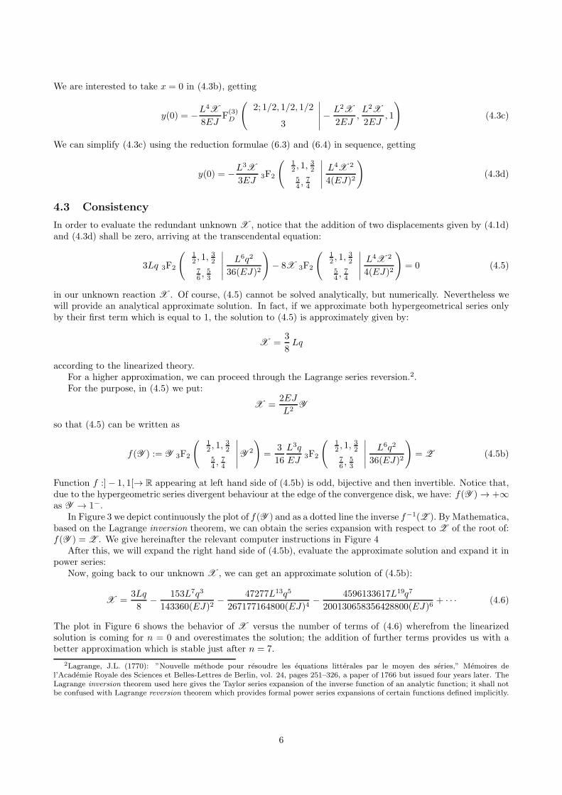
In Figure 3 we depict continuously the plot of f(Y ) and as a dotted line the inverse f−1(Z ). ByMathematica,based on the Lagrange inversion theorem, we can obtain the series expansion with respect to Z of the root of:f(Y ) = Z . We give hereinafter the relevant computer instructions in Figure 4

After this, we will expand the right hand side of (4.5b), evaluate the approximate solution and expand it inpower series:

Now, going back to our unknown X , we can get an approximate solution of (4.5b):

X =3Lq

8− 153L7q3

143360(EJ)2− 47277L13q5

267177164800(EJ)4− 4596133617L19q7

200130658356428800(EJ)6+ · · · (4.6)

The plot in Figure 6 shows the behavior of X versus the number of terms of (4.6) wherefrom the linearizedsolution is coming for n = 0 and overestimates the solution; the addition of further terms provides us with abetter approximation which is stable just after n = 7.

2Lagrange, J.L. (1770): ”Nouvelle methode pour resoudre les equations litterales par le moyen des series,” Memoires del’Academie Royale des Sciences et Belles-Lettres de Berlin, vol. 24, pages 251–326, a paper of 1766 but issued four years later. TheLagrange inversion theorem used here gives the Taylor series expansion of the inverse function of an analytic function; it shall notbe confused with Lagrange reversion theorem which provides formal power series expansions of certain functions defined implicitly.

6

Figure 3: f(Y ) and f−1(Z )

Figure 4: Series for Z = f−1(Y )

Figure 5: Approximate solution of (4.5b)

Figure 6: The statically indeterminate heavy cantilever supported by a roller with L = 1, q = 1000, EJ = 200,X values versus number of terms of its expansion

7

(a) (b)

L

A B

q

AB

X

qL/2

xy

A’ B’

A’’ B’’

X

(c)

x

y

+

(d)

y(0)>0

y(0)<0

B’

B’’

qL/2

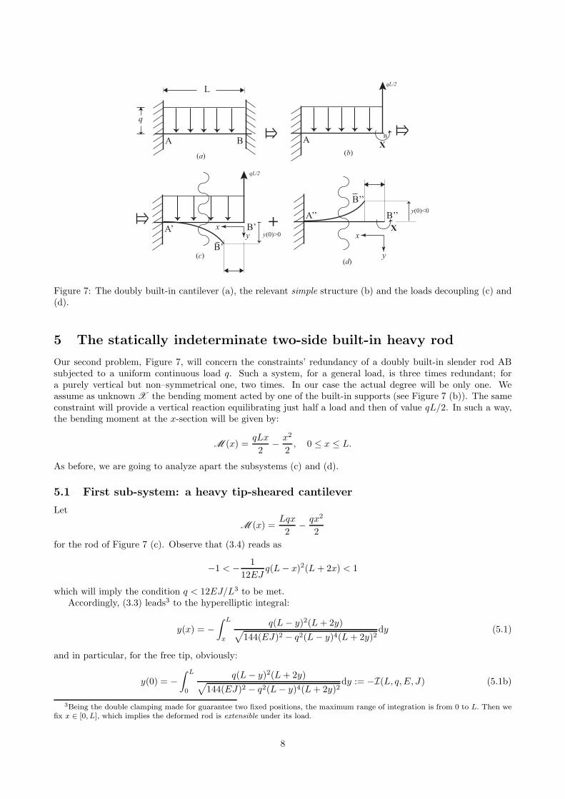
Figure 7: The doubly built-in cantilever (a), the relevant simple structure (b) and the loads decoupling (c) and(d).

5 The statically indeterminate two-side built-in heavy rod

Our second problem, Figure 7, will concern the constraints’ redundancy of a doubly built-in slender rod ABsubjected to a uniform continuous load q. Such a system, for a general load, is three times redundant; fora purely vertical but non–symmetrical one, two times. In our case the actual degree will be only one. Weassume as unknown X the bending moment acted by one of the built-in supports (see Figure 7 (b)). The sameconstraint will provide a vertical reaction equilibrating just half a load and then of value qL/2. In such a way,the bending moment at the x-section will be given by:

M (x) =qLx

2− x2

2, 0 ≤ x ≤ L.

As before, we are going to analyze apart the subsystems (c) and (d).

5.1 First sub-system: a heavy tip-sheared cantilever

Let

M (x) =Lqx

2− qx2

2

for the rod of Figure 7 (c). Observe that (3.4) reads as

−1 < − 1

12EJq(L− x)2(L + 2x) < 1

which will imply the condition q < 12EJ/L3 to be met.Accordingly, (3.3) leads3 to the hyperelliptic integral:

y(x) = −∫ L

x

q(L − y)2(L+ 2y)√

144(EJ)2 − q2(L− y)4(L + 2y)2dy (5.1)

and in particular, for the free tip, obviously:

y(0) = −∫ L

0

q(L− y)2(L+ 2y)√

144(EJ)2 − q2(L− y)4(L+ 2y)2dy := −I(L, q, E, J) (5.1b)

3Being the double clamping made for guarantee two fixed positions, the maximum range of integration is from 0 to L. Then wefix x ∈ [0, L], which implies the deformed rod is extensible under its load.

8

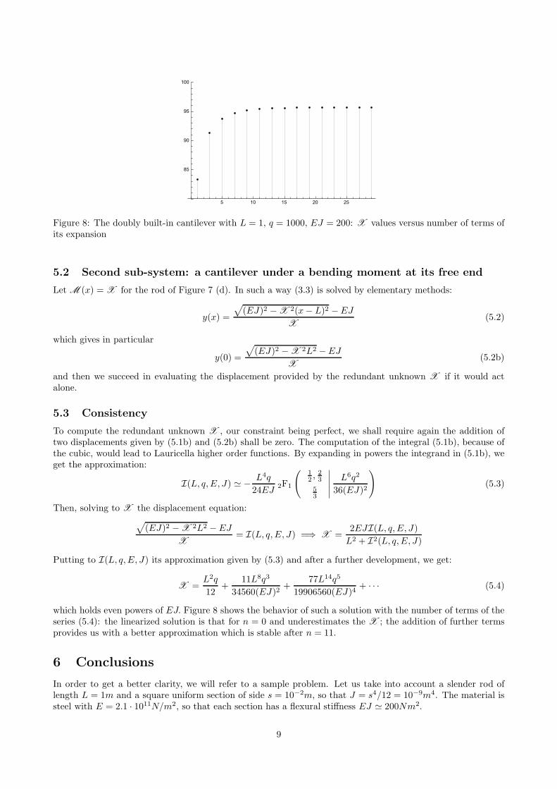
Figure 8: The doubly built-in cantilever with L = 1, q = 1000, EJ = 200: X values versus number of terms ofits expansion

5.2 Second sub-system: a cantilever under a bending moment at its free end

Let M (x) = X for the rod of Figure 7 (d). In such a way (3.3) is solved by elementary methods:

y(x) =

√

(EJ)2 − X 2(x− L)2 − EJ

X(5.2)

which gives in particular

y(0) =

√

(EJ)2 − X 2L2 − EJ

X(5.2b)

and then we succeed in evaluating the displacement provided by the redundant unknown X if it would actalone.

5.3 Consistency

To compute the redundant unknown X , our constraint being perfect, we shall require again the addition oftwo displacements given by (5.1b) and (5.2b) shall be zero. The computation of the integral (5.1b), because ofthe cubic, would lead to Lauricella higher order functions. By expanding in powers the integrand in (5.1b), weget the approximation:

I(L, q, E, J) ≃ − L4q

24EJ2F1

(

12 ,

23

53

∣

∣

∣

∣

∣

L6q2

36(EJ)2

)

(5.3)

Then, solving to X the displacement equation:

√

(EJ)2 − X 2L2 − EJ

X= I(L, q, E, J) =⇒ X =

2EJI(L, q, E, J)

L2 + I2(L, q, E, J)

Putting to I(L, q, E, J) its approximation given by (5.3) and after a further development, we get:

X =L2q

12+

11L8q3

34560(EJ)2+

77L14q5

19906560(EJ)4+ · · · (5.4)

which holds even powers of EJ. Figure 8 shows the behavior of such a solution with the number of terms of theseries (5.4): the linearized solution is that for n = 0 and underestimates the X ; the addition of further termsprovides us with a better approximation which is stable after n = 11.

6 Conclusions

In order to get a better clarity, we will refer to a sample problem. Let us take into account a slender rod oflength L = 1m and a square uniform section of side s = 10−2m, so that J = s4/12 = 10−9m4. The material issteel with E = 2.1 · 1011N/m2, so that each section has a flexural stiffness EJ ≃ 200Nm2.

9

Let us consider first the statically indeterminate unknown relevant to Figure 2 : according to the approximatelinear theory, it is given by 3qL/8, namely 375N for our sample problem. We take a unit continuous load ofq = 103N/m which is compliant to the prescription of being less than 6EJ/L3.

Our nonlinear approximate solution is provided by a relationship of kind (4.6), namely:

X =

∞∑

n=0

anL6n+1q2n+1

(EJ)2n

The reaction X of the statically indeterminate roller is then computed via a power series involving length, flex-ural rigidity, unit load and the relevant coefficients, some of which are shown by (4.6). Therefore Figure 6 showsthat the linearized approach overestimates about 7.8% the “reference value” provided by the (less approximate)nonlinear treatment which converges from n = 7 on.

Passing to the second statically indeterminate system (see Figure 7) we took the same unit continuousload q = 103N/m which is compliant to the new prescription of being less than 12EJ/L3. According to theapproximate linear theory, the statically indeterminate bending moment (hereinafter called again X ) exertedby one of the building-in constraints, is traditionally accepted as qL2/12, namely 83.33Nm for our sampleproblem. But a proper number of terms of (5.4)

X =

∞∑

n=0

bnL6n+2q2n+1

(EJ)2n,

provides a value of 95.16Nm which is 14.19% greater.The general conclusions suggested by all of the above are the following:

C1 In both problems analyzed in this paper, the traditional linearized approach leads to significant errors onthe statically unknowns. Such deviations increase for rods that are progressively more and more slenderand flexible, see Figure 6, Figure 8.

C2 The above mentioned effects obviously lead to a remarkable impact on the axial bending stresses, say σs. E.g. for the rod in Figure 2, the highest bending moment is given by X 2/2q and in that section therelevant edge σ is 16% lower than that from the linearized approach.

C3 For instance, referring to the rod in Figure 7, in the section of the highest moment, the relevant edge σ is6% greater than that from the linearized approach.

C4 It is commonly believed and written that the redundant unknowns do not depend on the flexural stiffness,but this is, generally speaking, not true.

In fact, our final formulae (4.6) and (5.4) show undoubtlessly that this is due to having taken n = 0, namelyonly the first term of the expansion whose subsequent terms hold the reciprocal of powers of EJ . Therefore theBelluzzi sentence, see [3] p. 363:

Si osservi che quando i vincoli sono rigidi la reazione A non dipende da EJ , mentre ne dipendequando sono cedevoli.4

can be accepted solely within a first order approximation.The linearized approach does its approximation at the very beginning of the treatment, so that leads to a less

refined and elementary conclusion. On the contrary, we keep the nonlinear nature of the problem, generatinga true solution which -even if we decide/need to approximate it at final stages- reveals new mathematical linksand conclusions.

Appendix: Hypergeometric identities

We recall hereinafter something about the non too known Lauricella hypergeometric functions.

4Notice that when the constraints are rigid, the (redundant) reaction does not depend upon EJ , whilst it does when theyundergo some yield.

10

The first hypergeometric series appeared in the Wallis’s Arithmetica infinitorum (1656):

2F1(a, b; c;x) = 1 +a · b1 · cx+

a · (a+ 1) · b · (b + 1)

1 · 2 · c · (c+ 1)x2 + · · · ,

for |x| < 1 and real parameters a, b, c. The product of n factors:

(λ)n = λ (λ+ 1) · · · (λ+ n− 1) ,

called Pochhammer symbol (or truncated factorial ) allows to write 2F1 as:

2F1(a, b; c;x) =

∞∑

n=0

(a)n (b)n(c)n

xn

n!.

A meaningful contribution on various 2F1 topics is ascribed to Euler5; but he does not seem [6] to have knownthe integral representation:

2F1(a, b; c;x) =Γ(c)

Γ(a)Γ(c− a)

∫ 1

0

ua−1(1− u)c−a−1

(1 − xu)bdu,

really due to A. M. Legendre6. The above integral relationship is true if c > a > 0 and for |x| < 1, even if thislimitation can be discarded thanks to the analytic continuation.

Furthermore, many functions have been introduced in 19th century for generalizing the hypergeometricfunctions to multiple variables. We recall the Appell F1 two–variable hypergeometric series, defined as:

F1

(

a; b1, b2

c

∣

∣

∣

∣

∣

x1, x2

)

=∞∑

m1=0

∞∑

m2=0

(a)m1+m2(b1)m1

(b2)m2

(c)m1+m2

xm1

1

m1!

xm2

2

m2!, |x1| < 1, |x2| < 1

The analytic continuation of Appell’s function on C \ [1,∞)×C \ [1,∞) comes from its integral representationtheorem: if Rea > 0, Re(c− a) > 0:

F1

(

a; b1, b2

c

∣

∣

∣

∣

∣

x1, x2

)

=Γ(c)

Γ(a)Γ(c− a)

∫ 1

0

ua−1 (1− u)c−a−1

(1− x1 u)b1 (1− x2 u)

b2du. (6.1)

For us, the functions introduced and investigated by G. Lauricella (1893) and S. Saran (1954), are of prevailing

interest; and among them the hypergeometric function F(n)D of n ∈ N+ variables (and n + 2 parameters), see

[16] and [10], defined as:

F(n)D (a, b1, . . . , bn; c;x1, . . . , xn) :=

∑

m1,...,mn∈N

(a)m1+···+mn(b1)m1

· · · (bn)mn

(c)m1+···+mnm1! · · ·mn!

xm1

1 · · ·xmm

n

with the hypergeometric series usual convergence requirements |x1| < 1, . . . , |xn| < 1.If Re c > Re a > 0 , the relevant Integral Representation Theorem (IRT) provides:

F(n)D (a, b1, . . . , bn; c;x1, . . . , xn) =

Γ(c)

Γ(a) Γ(c− a)

∫ 1

0

ua−1(1− u)c−a−1

(1− x1u)b1 · · · (1 − xnu)bndu

allowing the analytic continuation to Cn deprived of the cartesian n-dimensional product of the interval ]1,∞[with itself.

Finally, we provide here some reduction formulae employed throughout this paper.

F1

(

a; b, b,

a+ 1

∣

∣

∣

∣

∣

x,−x

)

= 2F1

(

a2 ; b,

a2 + 1

∣

∣

∣

∣

∣

x2

)

(6.2)

5We quote three works: a) De progressionibus transcendentibus, Op. omnia, S.1, vol. 28; b) De curva hypergeometrica Op.omnia, S.1, vol. 16; c) Institutiones Calculi integralis, 1769, vol. II

6A. M. Legendre, Exercices de calcul integral, II, quatrieme part, sect. 2, Paris 1811

11

Identity (6.2) follows from the integral representation theorem. In fact, if we return from the symbolic expressionfor the Appell function to its meaning in terms of integral representation, we see that

F1

(

a; b, b

a+ 1

∣

∣

∣

∣

∣

x, x

)

=Γ(a+ 1)

Γ(a)Γ(1)

∫ 1

0

ua−1

(1− x2u2)1/2du

= a

∫ 1

0

va2−1

(1− x2v)1/2dv = 2F1

(

a2 ; b,

a2 + 1

∣

∣

∣

∣

∣

x2

)

Next, we consider some generalizations of the well–known Gauss summation formula: if c > a+ b then

2F1

(

a; b

c

∣

∣

∣

∣

∣

1

)

=Γ(c)Γ(c− a− b)

Γ(c− a)Γ(c− b)

moreover, we also have

F1

(

a; b1, b2

c

∣

∣

∣

∣

∣

1, x

)

= 2F1

(

a; b1

c

∣

∣

∣

∣

∣

1

)

2F1

(

a; b2

c− b1

∣

∣

∣

∣

∣

x

)

which, when c > a+ b1 gives, due to the Gauss summation theorem,

F1

(

a; b1, b2

c

∣

∣

∣

∣

∣

1, x

)

=Γ(c)Γ(c− a− b1)

Γ(c− a)Γ(c− b1)2F1

(

a; b2

c− b1

∣

∣

∣

∣

∣

x

)

In similar way, it is possible to recognize the following formula, provided that c > a + b3, which we used tosimplify equation (4.1c).

F(3)D

(

a; b1, b2, b3

c

∣

∣

∣

∣

∣

x, y, 1

)

=Γ(c)Γ(c− a− b3)

Γ(c− a)Γ(c− b3)F1

(

a; b1, b2

c− b3

∣

∣

∣

∣

∣

x, y

)

(6.3)

We also recall the reduction formula7:

F1

(

a; b, b,

c

∣

∣

∣

∣

∣

x,−x

)

= 3F2

(

a+12 , a

2 , b

c+12 , c

2

∣

∣

∣

∣

∣

x2

)

(6.4)

Acknowledgements

The authors are indebted to their friend Prof. Aldo Scimone who drew some figures of this paper: they herebytake the opportunity to thank him warmly. The second author is supported by RFO Italian grant funding.

References

[1] M. Basoco. On the inflexional elastica. American Mathematical Monthly, pages 303–309, 1941.

[2] V. Beletsky and E. Levin. Dynamics of space tether systems, volume 83. Univelt Incorporated, San Diego,1993.

[3] O. Belluzzi. Scienza delle costruzioni, volume I. Zanichelli, Bologna, 1970.

[4] P. Burgatti. Teoria matematica dell’elasticita. Zanichelli, Bologna, 1931.

[5] R. De Pascalis, G. Napoli, and S. Turzi. Growth-induced blisters in a circular tube. Physica D, 283:1–9,2014.

[6] J. Dutka. The early history of the hypergeometric function. Archive for History of Exact Sciences, 31(1):15–34, 1984.

7 http://functions.wolfram.com/HypergeometricFunctions/AppellF1/03/05/

12

[7] R. Frisch-Fay. Flexible bars. Butterworths, London, 1962.

[8] V. Goss. The history of the planar elastica: insights into mechanics and scientific method. Science &

Education, 18(8):1057–1082, 2009.

[9] G. Greenhill. Graphical representation of the elliptic functions by means of a bent elastic beam. Messenger

of mathematics, 5:180–188, 1876.

[10] G. Lauricella. Sulle funzioni ipergeometriche a piu variabili. Rendiconti del Circolo Matematico di Palermo,7:111–158, 1893.

[11] J. A. L. Matheson. Hyperstatic structures: an introduction to the theory of statically indeterminate struc-

tures. Butterworths, London, 1971.

[12] G. Mingari Scarpello and D. Ritelli. Elliptic integral solutions of spatial elastica of a thin straight rod bentunder concentrated terminal forces. Meccanica, 41(5):519–527, 2006.

[13] G. Mingari Scarpello and D. Ritelli. Elliptic integrals solution to elastica’s boundary value problem of arod bent by axial compression. Journal of Analysis and Applications, 5(1):53–69, 2007.

[14] G. Mingari Scarpello and D. Ritelli. Elliptic functions solution to exact curvature elastica of a thin cantileverunder terminal loads. Journal of Geometry and Symmetry in Physics, 12(1):75–92, 2008.

[15] G. Mingari Scarpello and D. Ritelli. Exact solutions of nonlinear equation of rod deflections involving theLauricella hypergeometric functions. International Journal of Mathematics and Mathematical Sciences,2011, 2011.

[16] S. Saran. Hypergeometric functions of three variables. Ganita, 5:77–91, 1954.

[17] W. Schell. Theorie der Bewegung und der Krafte. B.G. Teubner, Leipzig, 1870.

[18] F. G. Tricomi. Funzioni ellittiche. Zanichelli, Bologna, 1951.

[19] T. Wagner and D. Vella. The sticky elastica: the lamination blisters beyond small deformations. Soft

Matter, 9:1025–130, 2013.

13