agriculture and adaptation in bangladesh -...

IFPRI Discussion Paper 01281

July 2013

Agriculture and Adaptation in Bangladesh

Current and Projected Impacts of Climate Change

Timothy S. Thomas

Khandaker Mainuddin

Catherine Chiang

Aminur Rahman

Anwarul Haque

Nazria Islam

Saad Quasem

Yan Sun

Environment and Production Technology Division

INTERNATIONAL FOOD POLICY RESEARCH INSTITUTE

The International Food Policy Research Institute (IFPRI), established in 1975, provides evidence-based policy solutions to sustainably end hunger and malnutrition and reduce poverty. The Institute conducts research, communicates results, optimizes partnerships, and builds capacity to ensure sustainable food production, promote healthy food systems, improve markets and trade, transform agriculture, build resilience, and strengthen institutions and governance. Gender is considered in all of the Institute’s work. IFPRI collaborates with partners around the world, including development implementers, public institutions, the private sector, and farmers’ organizations, to ensure that local, national, regional, and global food policies are based on evidence. IFPRI is a member of the CGIAR Consortium.

AUTHORS Timothy S. Thomas, International Food Policy Research Institute Research Fellow, Environment and Production Technology Division [email protected] Khandaker Mainuddin, Bangladesh Centre for Advanced Studies Senior Fellow

Catherine Chiang, Consultant Formerly a research analyst in IFPRI’s Environment and Production Technology Division

Aminur Rahman, Bangladesh Centre for Advanced Studies Senior Research Officer

Anwarul Haque, Bangladesh Centre for Advanced Studies Senior Agricultural Specialist

Nazria Islam, Bangladesh Centre for Advanced Studies Senior Research Officer

Saad Quasem, Bangladesh Centre for Advanced Studies Former Research Officer

Yan Sun, Consultant Formerly a research analyst in IFPRI’s Environment and Production Technology Division

Notices 1. IFPRI Discussion Papers contain preliminary material and research results. They have been peer reviewed, but have not been subject to a formal external review via IFPRI’s Publications Review Committee. They are circulated in order to stimulate discussion and critical comment; any opinions expressed are those of the author(s) and do not necessarily reflect the policies or opinions of IFPRI. 2. The boundaries and names shown and the designations used on the map(s) herein do not imply official endorsement or acceptance by the International Food Policy Research Institute (IFPRI) or its partners and contributors.

Copyright 2013 International Food Policy Research Institute. All rights reserved. Sections of this material may be reproduced for personal and not-for-profit use without the express written permission of but with acknowledgment to IFPRI. To reproduce the material contained herein for profit or commercial use requires express written permission. To obtain permission, contact the Communications Division at [email protected].

mailto:[email protected]

Contents

Acknowledgments vi

Abstract vii

Abbreviations and Acronyms viii

1. Introduction 1

2. Using Models to Assess the Impact of Climate Change on Agriculture 9

3. Household Survey 36

4. Conclusions and Recommendations 60

References 62

iii

Tables

1.1—Climatic elements, critical vulnerable areas, impacted sectors, and links with PRSP and MDGs 4 1.2—Present and future impacts of different climatic events on crop agriculture, poverty, and

economic growth 5 2.1—Mean annual precipitation: Level for 2000 and changes between 2000 and 2050 15 2.2—Precipitation of the wettest three months: Level for 2000 and changes between 2000 and 2050 15 2.3—Normal daily maximum temperature for warmest month: Level for 2000 and changes between

2000 and 2050 16 2.4—Summary of climate change impacts between 2000 and 2050, by GCM 16 2.5—Changes in rainfed aman yields from 2000 to 2050, median change 23 2.6—Changes in irrigated boro yields from 2000 to 2050, median change 26 2.7—Changes in crop yields from 2000 to 2050, median value from all four GCMs 27 2.8—Yield response from supplementing nitrogen in the soil 28 2.9—Harvest area and production of major crops in Bangladesh 28 2.10—Percent changes in world prices of food commodities, 2000 to 2050 33 3.1—SRDI’s 30 agroecological zones, grouped into 7 agroecological zones. 36 3.2—Number of unions and households per AEZ covered in the household survey 37 3.3—Percentage distribution of gender of household head, by AEZ 38 3.4—Percentage distribution of marital status of household head, by AEZ 38 3.5—Mean household size, and mean age and years of schooling of household head, by AEZ 39 3.6—Highest class passed by household head (percent) 39 3.7—Households’ owned land size class versus operated land size class (number of households) 40 3.8—Households’ average farm size and number of plots, by AEZ 40 3.9—Average household rice plot size by AEZ 41 3.10—Planting date for each type of rice (plot level) 42 3.11—Households’ fertilizer use by operated land size class (for rice only) 42 3.12—Households’ fertilizer use by AEZ (for rice only) 43 3.13—Households’ pesticide use (rice only) by operated land size class 43 3.14—Households’ pesticide use (rice only) by AEZ 44 3.15—Rice yield by operated land size class 44 3.16—Households’ rice paddy loss by operated land size class (loss in percent) 45 3.17—Distribution of rice loss, by cause of loss and AEZ 45 3.18—Proportion of rice loss to total potential production, by cause of loss and AEZ 46 3.19—Estimation result from regression (dependent variable is log of yield) 47 3.20—Top three types of crop rotation, by AEZ 48 3.21—Proportion of households that used various methods of tillage, by AEZ 48 3.22—Proportion of households that used animal manure and green manure, by AEZ 49 3.23—Proportion of households that practiced various land management practices (percentage), by

AEZ 49 3.24—Agricultural extension by operated land size class (household level) 50 3.25—Agricultural extension by AEZ 50 3.26—Perceived level of losses by farms affected by three main hazards (percent) 52 3.27—Loss of production by hazard type and by crop (MT) 52 3.28—Top three noticed changes in climate in the last 20 years, by AEZ 53 3.29—Recommended dosage of fertilizer for rice and level of actual fertilizer usage 55 3.30—Top three adaptation measures, by AEZ 57 3.31—Summary statistics of independent variables 57 3.32—Results of the probit adaptation model, marginal effects reported 58

iv

Figures

1.1—The six divisions of Bangladesh used in this report 2 2.1—Average annual rainfall, in millimeters, 1950–2000 9 2.2—Average annual high temperature, degrees Celsius, 1950–2000 10 2.3—Changes in important climate indicators, 2000 to 2050, for CNRM-CM3 GCM, A1B scenario 11 2.4—Changes in important climate indicators, 2000 to 2050, for CSIRO-MK3 GCM, A1B scenario 12 2.5—Changes in important climate indicators, 2000 to 2050, for ECHAM5 GCM, A1B scenario 13 2.6—Changes in important climate indicators, 2000 to 2050, for MIROC3.2 medium-resolution GCM,

A1B scenario 14 2.7—Mean daily high and low temperatures by month and division, degrees Celsius 17 2.8—Mean monthly precipitation by division, in millimeters 18 2.9—Mean monthly number of rainy days by division 19 2.10—Mean daily solar radiation by month and division, mJ/m2/day 20 2.11—Change in yield of rainfed aman rice, high fertilizer levels, 2000 to 2050, with optimal

planting date and variety for 2000 and the same date and variety used in 2050 21 2.12—Change in yield of rainfed aman rice, high fertilizer levels, 2000 to 2050, with optimal

planting date and variety for both 2000 and 2050 22 2.13—Change in yield of irrigated boro rice, high fertilizer levels, 2000 to 2050, with optimal

planting date and variety for 2000 and the same date and variety used in 2050. 24 2.14—Change in yield of irrigated boro rice, high fertilizer levels, 2000 to 2050, with optimal

planting date and variety for both 2000 and 2050 25 2.15—Projected GDP per capita 30 2.16—Projected population 30 2.17—Food price projections 31 2.18—Malnutrition projections for children under five years of age 33 2.19—Yield projections for rice 33 2.20—Harvest area projections for rice 34 2.21—Production projections for rice 34 2.22—Net export projections for rice 35 3.1—Map of study sites 37 3.2—Percentage of respondents whose agricultural land/harvest had been affected by a natural hazard

in the last five years 51 3.3—Percentage of respondents whose agricultural harvest/land had been affected by natural hazards

in the last five years, by type of hazard 51 3.4—Farmers’ perception of changes in climate over the last 20 years, by AEZ 52 3.5—Specific changes in climate noticed in the last 20 years, by percentage of farmers reporting 53 3.6—Percentage of farm households reporting adaptation to perceived long-term changes in

temperature and rainfall, by AEZ 54 3.7—Changes in agricultural practices in response to perceived climate change, by percentage of

farmers reporting 55 3.8—Adaptation strategies reported, by AEZ (percentage of farmers reporting) 56

v

ACKNOWLEDGMENTS

This research was funded by the United States Agency for International Development (USAID) and conducted under the CGIAR Research Program on Climate Change, Agriculture, and Food Security (CCAFS). The BanglaSPAM mapping used in this study was also supported by the Bangladesh Policy Research and Strategy Support Program, which is also financially supported by USAID.

vi

ABSTRACT

Bangladesh is extremely vulnerable to the impact of climate change because it is a low-lying, flat country subject to both riverine flooding and sea level rise, and because a large portion of its population is dependent on agriculture for its livelihood. The goal of this research was to examine the likely impacts of climate change on agriculture in Bangladesh, and develop recommendations to policymakers to help farmers adapt to the changes. In this study, we use climate data from four general circulation models (GCMs) to evaluate the impact of climate change on agriculture in Bangladesh by 2050. We use the DSSAT (Decision Support System for Agrotechnology Transfer) crop modeling software to evaluate crop yields, first for the 1950 to 2000 period (actual climate) and then for the climates given by the four GCMs for 2050. We evaluate crop yields at 1,789 different points in Bangladesh, using a grid composed of roughly 10 kilometer (km) squares, for 8 different crops in 2000 and 2050. For each crop, we search for the best cultivar (variety) at each square, rather than limiting our analysis to a single variety for all locations. We also search for the best planting month in each square. In addition, we explore potential gains in changing fertilizer levels and in using irrigation to compensate for rainfall changes. This analysis indicates that when practiced together, using cultivars better suited for climate change and adjusting planting dates can lessen the impacts of climate change on yields, especially for rice, and in some cases actually result in higher yields. In addition, the analysis shows that losses in yield due to climate change can be compensated for, for many crops, by increasing the availability of nitrogen in the soil. Moreover, we used a household survey to collect information on the incidence of climatic shocks in the last five years and adaptation options. The survey was conducted from December 2010 to February 2011, covering data from the previous production year. The results confirm that Bangladesh farmers already perceive the impacts of climate change. In particular, the survey results indicate that of all climate change–related shocks, floods, waterlogging, and river erosion caused the largest loss to rice production. Farmers in our survey lost around 12 percent of their harvest, on average, to some kind of shock, with about half of that attributable to flooding-related issues. The second leading cause of rice crop loss was pests, responsible for around 3 percent of production. Taken together, the results indicate that adaptation efforts in Bangladesh should include adjusting planting dates, using improved cultivars better suited for climate change, improving fertilizer application, exploring increased maize production, and bolstering flood and pest protection for farmers.

Keywords: climate change, IMPACT model, GCM, Bangladesh, adaptation, agriculture

vii

ABBREVIATIONS AND ACRONYMS

ADB Asian Development Bank AEZ agroecological zone BanglaSPAM Bangladesh spatial production allocation model DSSAT Decision Support System for Agrotechnology Transfer CNRM-CM3 Centre National de Recherches Météorologiques Coupled Global Climate Model,

version 3 CSIRO-Mk3 Commonwealth Scientific and Industrial Research Organisation model, version Mk3 ECHAM5 European Centre–Hamburg model, version 5 GCM general circulation model GDP gross domestic product IMPACT International Model for Policy Analysis of Agricultural Commodities and Trade IPCC International Panel on Climate Change K potassium MDG Millennium Development Goals MIROC3.2 Model for Interdisciplinary Research on Climate, version 3.2 N nitrogen NAPA National Adaptation Programme of Action P phosphorus PRSP Poverty Reduction Strategy Paper SPAM spatial production allocation model SRDI Soil Resources Development Institute USG urea super granules USAID United States Agency for International Development

viii

1. INTRODUCTION

Many in the scientific and development communities are concerned that the combination of climate change and population growth in many developing countries threatens to become the perfect storm, whereby the combination of reduced food supply due to climate effects on agriculture and increased demand from still-growing populations might validate Malthus’s fears, resulting in food shortages and widespread hunger.

Yet despite food crises in recent years that resulted in riots in many cities around the globe, it is not clear that the fears concerning the impact of climate change and population growth are warranted. Technological growth in the agricultural sector, including the Green Revolution of recent decades, along with some expansion of agricultural land, has managed to generally supply the world’s population with sufficient food despite explosive population growth in the last century. Clearly large portions of the global population still struggle with gaining access to sufficient nutrition, but these struggles seem to come not from insufficient production of food but from constraints on poor people’s gaining access to the existing food due to poverty and, sometimes, distribution failures.

Bangladesh is extremely vulnerable to the impact of climate change, in part because it is a low-lying and very flat country, subject to riverine flooding and vulnerable to sea level rise. The confluence of three great rivers—the Ganges, the Brahmaputra, and the Meghna—makes the country a great deltaic plain. The extensive floodplains are the main physiographic features of the country. Both riverine flooding and sea level rise can result in inundation of crops; sea water, in particular, can result in salinization, causing permanent loss of currently productive agricultural land.

The climate of Bangladesh is characterized by high temperatures, heavy rainfall, high humidity, and fairly marked seasonal variations. More than 80 percent of the annual precipitation of the country occurs during the southwestern summer monsoons, from June through September. In recent years the weather pattern has been erratic, with the cool, dry season having considerably decreased—a change probably attributable to climate change.

Climate change, by definition, will alter temperature and rainfall patterns. Since agriculture is dependent on weather and crops are known to suffer yield losses when temperatures are too high, there is concern that warming caused by climate change will lower crop yields. Changes in rainfall might also cause reductions in yields, though at least in some places, changes in rainfall could lead to increases in yields.

Climate change in Bangladesh is an especially serious concern since agriculture is such an important sector in the country. It contributes roughly 20 percent to gross domestic product (GDP), with crops representing 11.2 percent, livestock 2.7 percent, fisheries 4.5 percent, and forestry 1.8 percent (Bangladesh, Ministry of Finance 2011). Furthermore, the sector provides employment and income to some of the poorest and most vulnerable members of society. Between 2000 and 2003, agriculture provided work to about 52 percent of the labor force (BBS 2004).

While there has been significant progress in the area of poverty reduction, Bangladesh is still in the bottom quintile of the nations of the world in GDP per capita, indicating that it has limited resources to adapt to climate shocks and is therefore vulnerable to even moderate changes. Bangladesh covers an area of 147,570 sq. km and is one of the most densely populated countries in the world. The total population of the country in 2009 was estimated at 146.6 million, with a population density of 993 per sq. km.

Figure 1.1 shows the divisions of Bangladesh used in this study, which are the divisions that existed up until January 2010. At the end of January 2010, Rajshahi division was split in two, with the northern part becoming Rangupur division.

1

Figure 1.1—The six divisions of Bangladesh used in this report

Source: Authors.

Previous Studies of Climate Change Impacts on Agriculture Many studies of the impact of climate change on agriculture have already been conducted. Hertel and Rosch (2010) reviewed a number of these, as did Tubiello and Rosenzweig (2008). Hertel and Rosch (2010) highlighted three major approaches to assessing the impacts: crop growth simulation models, estimates of statistical relationships between crop yields and climate variables (precipitation and temperature), and hedonic or Ricardian models. The current study uses crop modeling. A large number of studies have used this approach for various regions of the world: White and colleagues (2011) reviewed 221 papers on the use of crop models in assessing the impact of climate change on agriculture.

The Asian Development Bank (ADB) and the International Food Policy Research Institute (IFPRI) studied the impact of climate change on agriculture in the countries of Asia and the Pacific, concluding that “a combination of indicator values representing exposure (change in temperature and precipitation), sensitivity (share of labor in agriculture), and adaptive capacity (poverty) identifies Afghanistan, Bangladesh, Cambodia, India, Lao PDR, Myanmar, and Nepal as the countries most vulnerable to climate change” (ADB and IFPRI 2009, p 9). They went on to suggest that “required public agricultural research, irrigation, and rural road expenditures are estimated to be [US]$3.0–$3.8 billion annually during 2010–2050, above and beyond projected baseline investments. In addition, these agricultural investments require complementary investments in education and health, estimated at $1.2 billion annually up to 2050” (2009, p. 20).

ADB and IFPRI (2009) used a methodology very similar to that of some global studies, including studies by Nelson, Rosegrant, Koo, et al. (2009, 2010) and Nelson, Rosegrant, Palazzo, et al. (2010). Our study takes a more detailed look at the impact of climate change on agriculture in Bangladesh, using an approach similar to that of ADB and IFPRI (2009) but extending it in many important ways. First, our modeling approach differs slightly. Instead of restricting the analysis to areas already growing the particular crop, we examine the potential viability of the crop on all land areas. This approach allows us to

2

consider the feasibility of expanding a crop into new areas or bringing in a crop not currently grown. Second, we analyze potential yield for every variety available within the Decision Support System for Agrotechnology Transfer (DSSAT), rather than a single variety (or two, in the case of rice) as in other studies. Third, we allow the planting date to move freely (except when examining crops that are specific to the wet season or dry season, where we restrict the months as appropriate). By allowing the planting date to shift radically, we consider wider adaptation options than do the other studies. Fourth, we consider a wider range of crops. Fifth, we consider a wider range of fertilizer application options. Sixth, we use newer climate models than the ones used by ADB and IFPRI (2009); Nelson, Rosegrant, Koo, et al. (2009); and Nelson, Rosegrant, Palazzo, et al. (2010). Our models are the same ones used by Nelson, Rosegrant, Palazzo, et al. (2010). Seventh, our spatial resolution is much finer than that of the other studies. The three studies using the older climate models had a spatial resolution of roughly 60 km; Nelson, Rosegrant, Koo, et al (2010) had a resolution of roughly 30 km; we use a spatial resolution of 10 km. Finally, we include detailed information about the national context, including agriculture, the environment, and overall economic development, as well as the policy environment.

Masutomi et al. (2009) studied the impact of climate change on rice in Asia using DSSAT, the same crop model software used here, with 19 general circulation models (GCMs). Their analysis used a wider collection of GCMs (we use just 4) and of emissions scenarios (they used three while we use one); they also used a varied time frame that included estimates for 2030, 2050, and 2080, while we focus on 2050. However, their spatial resolution was 144 times lower than ours (12 times in both horizontal and vertical directions, at a 1 degree resolution). They analyzed only two varieties of rice, with no option of selecting a new variety in adapting to climate change. They did consider different growing periods and allowed for planting dates to be changed.

Our approach is complementary to the study by Yu et al. (2010), a very important analysis of the impact of climate change on agriculture in Bangladesh. In both studies, the DSSAT crop modeling software is used to evaluate crop yields for the climate of the period from 1950 to 2000 as well as for climate change projections as modeled by multiple GCMs. This report analyzes changes for the year 2050; Yu et al.(2010) presented an analysis for 2080 as well. Yu et al. (2010) used 16 models rather than 4, and three climate scenarios rather than one, giving a broader range of predictions. However, that analysis was limited to 16 geographic points, while we evaluate crop yields at almost 2,000 points, using a grid of 10 km squares (approximately).1 Furthermore, that analysis covered only rice and wheat, while ours examines eight different crops (including rice and wheat).

Our approach differs markedly from the approach used in previous studies in that we explore the possibility of substituting cultivars2 that are better suited to the future climate, and we allow for changing the planting month to make it more optimal for the future climate. We also explore potential gains from changing fertilizer levels, and using irrigation to compensate for any deficits from rainfall changes.

Climate Change Impacts on Poverty and Economic Growth The relationship among climate change, poverty, economic growth, and sustainable development is multidimensional and complex. It is recognized in the scientific and development community that climate change–induced impacts will create additional challenges for achieving many of the Millennium Development Goals (MDGs) and targets in general, particularly regarding poverty, hunger, and environmental sustainability. The National Adaptation Programme of Action of Bangladesh shows that climatic elements will impact different sectors and geographic areas on a different scale. A policy study on the probable impacts of climate change on poverty and economic growth in Bangladesh revealed that a

1 They are actually squares of 5 arc minutes, which vary in length of each side depending upon the distance from the equator. We round up to 10 km for ease of understanding.

2 We define an optimal cultivar at a given pixel as one that leads to the highest average yield over multiple weather distributions based on the given climate. The cultivars are chosen among those available in the DSSAT program, which reflect existing cultivars. Future research is expected to produce cultivars that will give even higher yields in climates of the future, pointing to the importance of continued research.

3

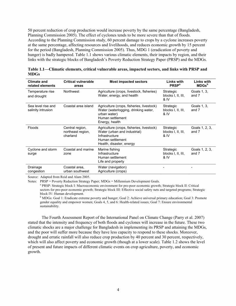
50 percent reduction of crop production would increase poverty by the same percentage (Bangladesh, Planning Commission 2005). The effect of cyclones tends to be more severe than that of floods. According to the Planning Commission study, 60 percent damage to crops by a cyclone increases poverty at the same percentage, affecting resources and livelihoods, and reduces economic growth by 15 percent for the period (Bangladesh, Planning Commission 2005). Thus, MDG 1 (eradication of poverty and hunger) is badly hampered. Table 1.1 shows various climatic elements, their impacts by region, and their links with the strategic blocks of Bangladesh’s Poverty Reduction Strategy Paper (PRSP) and the MDGs.

Table 1.1—Climatic elements, critical vulnerable areas, impacted sectors, and links with PRSP and MDGs

Climate and related elements

Critical vulnerable areas

Most impacted sectors Links with PRSPa

Links with MDGsb

Temperature rise and drought

Northwest

Agriculture (crops, livestock, fisheries) Water, energy, and health

Strategic blocks I, II, III, & IV

Goals 1, 3, and 7

Sea level rise and salinity intrusion

Coastal area island Agriculture (crops, fisheries, livestock) Water (waterlogging, drinking water, urban water) Human settlement Energy, health


Goals 1, 3, and 7

Floods Central region, northeast region, charland

Agriculture (crops, fisheries, livestock) Water (urban and industrial) Infrastructure Human settlement Health, disaster, energy


Goals 1, 2, 3, and 7

Cyclone and storm surge

Coastal and marine zone

Marine fishing Infrastructure Human settlement Life and property


Goals 1, 2, 3, and 7

Drainage congestion

Coastal area, urban southwest

Water (navigation) Agriculture (crops)

- -

Source: Adapted from Reid and Alam 2005. Notes: PRSP = Poverty Reduction Strategy Paper; MDGs = Millennium Development Goals.

a PRSP: Strategic block I: Macroeconomic environment for pro-poor economic growth; Strategic block II: Critical sectors for pro-poor economic growth; Strategic block III: Effective social safety nets and targeted programs; Strategic block IV: Human development. b MDGs: Goal 1: Eradicate extreme poverty and hunger; Goal 2: Achieve universal primary education; Goal 3: Promote gender equality and empower women; Goals 4, 5, and 6: Health-related issues; Goal 7: Ensure environmental sustainability.

The Fourth Assessment Report of the International Panel on Climate Change (Parry et al. 2007) stated that the intensity and frequency of both floods and cyclones will increase in the future. These two climatic shocks are a major challenge for Bangladesh in implementing its PRSP and attaining the MDGs, and the poor will suffer more because they have less capacity to respond to these shocks. Moreover, drought and erratic rainfall will also reduce crop production by 40 percent and 30 percent, respectively, which will also affect poverty and economic growth (though at a lower scale). Table 1.2 shows the level of present and future impacts of different climatic events on crop agriculture, poverty, and economic growth.

4

Table 1.2—Present and future impacts of different climatic events on crop agriculture, poverty, and economic growth

Climatic event

Level of impact (%) Identified impacts Poverty Economic growth

Present Future (2100)



Flood 50 80 50 80 12 17 Drought 25 40 08 30 02 05 Cyclone 60 70 60 70 15 17 Coastal inundation 10 15 05 08 01 02 Erratic rainfall 20 30 10 20 02 04 Temperature variation 05 07 02 05 02 02 Heat wave - 02 - 01 - 01 Fog 10 15 02 03 01 01

Source: UNDP 2009.

Flood, riverbank erosion, cyclone, and storm surge have severe impacts on fisheries, with moderate effects on poverty and economic growth. These shocks damage aquaculture infrastructure and cause fish loss, leading to loss of livelihoods of poor fishers and decreasing the nutrition status of the rural poor. Moreover, frequent cyclone warnings lead fishers to stay at home for longer periods, lowering their income. In addition, drought, salinity intrusion, and erratic rainfall affect the fisheries sector moderately. Severe impacts of flood, drought, cyclone, and storm surge, as well as sea level rise and salinity intrusion, will severely affect the poverty of this livelihood group. The growth of the fisheries sector will also be affected moderately.

Livestock rearing is an important source of income and livelihood options for the rural poor of Bangladesh. The impact of climate change on livestock is expected to reduce livelihood opportunities, income, and employment opportunities of poor villagers. Sea level rise will have severe effects on poverty and the economic growth of this sector; drought, salinity intrusion, and heat wave will affect the sector moderately.

Livelihoods of the poor and marginal communities in the forest areas, especially in the Sundarbans area, mostly depend on forest resources. Salinity intrusion severely affects forest resources, especially in the coastal region, with moderate impacts on poverty and economic growth. Flood and drought will have moderate impacts on forestry, with low impacts on poverty and economic growth; erratic rainfall and temperature variation will have low impacts on forestry and lower impacts on poverty. Sea level rise is likely to affect forest coverage in the coastal areas very severely, through submergence of brackish forest species and disappearance of inland trees and plants. Flood, cyclone, and salinity intrusion are likely to have severe impact on forest resources, with severe effects on poverty in the affected areas.

Model In a simple way of thinking about crop growth, we might say that the yield from a given piece of land is a function of just a few things: seed variety (V); soil characteristics (N), including nutrients; water availability (H); temperature (T); and sunshine (S). Except for seed variety, which is fixed once selected, the other elements vary moment by moment. We could write a simple yield function as

𝑦(𝑁,𝐻,𝑇, 𝑆;𝑉). (1)

The variety determines how all the other inputs affect yield, so we treat it differently by putting it after the semicolon.

5

There is a time dimension to yield—that is, the number of days that pass between the time the seed (or seedling) is planted and the time the crop is harvested. Yield is affected by the variable factors (nutrients, water, temperature, and sunshine) over the whole period from planting to harvesting. Because crop growth is sensitive to temperature (as well as changes in nutrients, water, and sunshine), with growing rate changing markedly throughout the day depending on the temperature, it would be more accurate to factor in the changes in temperature (as well as in the other variables) as inputs—ideally, perhaps, a different temperature for every hour over the growing period.

Crops can be sensitive to both high and low temperatures. There are a few measures a farmer can take in some instances to modify the impact of temperatures (such as covering plants to prevent them from freezing, as is sometimes done for high-value crops), but for field crops generally there are no economically viable interventions. In regard to temperature, the main variables that the farmer controls are the planting date, d, and harvest date, h. If the farmer were able to see in advance the weather (including the temperature profile) of an entire year, the farmer would be able to choose the ideal planting and harvest dates to maximize yield. The farmer would also be able to choose a more ideal variety to plant. For example, if the year ahead showed many days with high temperatures during the growing season, the farmer might choose a heat-tolerant variety, whose growth would not be hindered by heat as much as standard varieties of the crop. We might write this temperature function as

𝑇(𝑡;𝑑,ℎ), (2)

where t is time. Unfortunately, in reality the farmer does not have the ability to know in advance the daily and

hourly temperatures of the coming year, so she instead forms expectations about those things. Traditionally those expectations are based on the farmer’s knowledge of the long-term climate conditions of her area, given by C. That is, she will be aware of the typical temperature ranges of each month of the year (perhaps even each week of the year), along with some idea of how extreme these temperature have been in the past.

Science continues to develop in its accuracy for shorter-term predictions of weather. Longer-term, seasonal predictions (4 to 6 months in advance) are also becoming more accurate for many regions of the world, based on, among other things, the El Niño Southern Oscillation. Seven-day weather forecasts (C7) and 120-day weather outlooks (C120) influence and improve the farmer’s expectations for weather. The weather outlook might help the farmer better choose the variety of seed to plant and perhaps influence other crop husbandry decisions. The weather forecast can help the farmer to pinpoint planting and harvest dates, particularly in order to avoid overly water-saturated fields and to select dates when the crop (which is often allowed to dry in the field) can be harvested without getting wet again from rain. The temperature function can now be expanded as 𝐸[𝑇(𝑡;𝑑, ℎ);𝐶,𝐶7,𝐶120], (3)

where E is the expectation operator. When we write the function this way, we are looking at the problem from the farmer’s perspective. The previous temperature function defined actual temperature rather than expected temperature, looking from the crop modeler’s perspective.

We can write an identical set of functions for sunshine. However, the set of functions for water availability is a little more complicated. Temperature and sunshine cannot be modified by the farmer (except by choice of the planting and harvest dates); water availability in some circumstances can be modified by the farmer, through water application; that is, in addition to dependency on rainfall, R, the farmer in some cases can use irrigation, I, which we express as a function of time, because water can be applied at specific dates with specific levels of water added:

𝐻(𝑅(𝑡), 𝐼(𝑡);𝑑,ℎ). (4)

6

It is not as clear whether we should consider soil nutrients as a function of weather or a function of time or both. More rainfall and more intensive rain can make some nutrients less available to crops by causing them either to run off (if fertilizer has been used) or to go deeper than the roots can access. And over the course of a growing season, as the plant uses nutrients, they will no longer remain in the soil. Nutrient uptake will also vary based on the crop and crop variety. Furthermore, because crop growth is affected by many nutrients, N should be thought of as a vector of nutrients. Soil type (D) helps determine the amount of nutrients a soil can hold as well as the rate of loss of those nutrients.

Soil nutrients can be modified through application of organic fertilizers (such as compost or manure) and inorganic fertilizers, F, just as water availability can be modified through irrigation. We might also think of other soil amendments, such as gypsum (to adjust pH) or rhizobia (to enhance nitrogen fixation), but these can be incorporated into F, which is best thought of as a vector. (Consider that fertilizers can add to the soil nitrogen, phosphorus, potassium, sulfur, and various micronutrients.) We might write the nutrient function as

𝑁�𝑡,𝐹(𝑡);𝑑,ℎ,𝑉,𝐷,𝑅(𝑡)�. (5)

We have omitted for the purpose of simplification other major crop-related issues. First is the issue of weeds, which we might model similarly to soil nutrients because weeds can be reduced either through herbicides or through weeding (mechanical processes). Similarly, insects and other pests can affect yield, and their impact can be modified through insecticides and other interventions. A function similar to that used for soil nutrients could be used for weeds and pests. Or, thinking more broadly about soil nutrients as the soil- and plant-supporting environment, we could easily fold weeds and pests into the vector for soil nutrients (but bearing in mind that more weeds and pests lead to worse yields, while more nutrients lead to better yields). Accordingly, we might fold the interventions—herbicides, pesticides, and weeding—into an intervention vector, previously limited to fertilizer application. For simplicity, however, we will not further address weeds and pests in the modeling section of the paper.

The yield function is now a lot more complicated:

𝑦�𝑁�𝑡,𝐹(𝑡);𝑑,ℎ,𝑉,𝐷,𝑅(𝑡)�,𝐻(𝑅(𝑡), 𝐼(𝑡);𝑑,ℎ),𝑇(𝑡;𝑑, ℎ),𝑆(𝑡;𝑑,ℎ);𝑉�. (6)

A reduced form of this would be

𝑦�𝑑,ℎ,𝑉,𝐹(𝑡), 𝐼(𝑡);𝐷,𝑅(𝑡),𝑇(𝑡), 𝑆(𝑡)�. (7)

Essentially, this function groups the variables selected by the farmer (or modeler) before the semicolon; following the semicolon are the variables that are out of the farmer’s (modeler’s) hands, which are soil type and weather factors.

In practice, the farmer must choose the planting date, d, and the seed variety, V, before beginning cultivation. Harvest date, h; fertilizer application, F; and irrigation, I, can be chosen later (though starter fertilizer and starter irrigation would normally be chosen ahead of time). In terms of the modeling done in this report, h chooses itself: We can tell the program to harvest when the crop is mature (similar to the way a farmer decides). This strategy would reduce the yield function further to

𝑦�𝑑,𝑉,𝐹(𝑡), 𝐼(𝑡);𝐷,𝑅(𝑡),𝑇(𝑡), 𝑆(𝑡)�. (8)

The other variables (planting date; crop variety; and whether, how much, and when to apply fertilizer and irrigation) have to be set before running the program. The soil type at each point of analysis is inserted, along with climate variables that allow the program to simulate daily values of rainfall, temperature, and solar radiation.

7

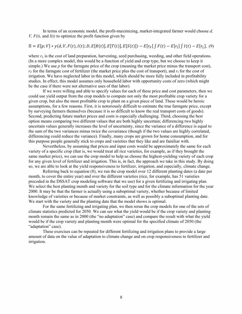
In terms of an economic model, the profit-maximizing, market-integrated farmer would choose d, V, F(t), and I(t) to optimize the profit function given by

Π = 𝐸[𝑝;𝑉] ∗ 𝑦(𝑑,𝑉,𝐹(𝑡), 𝐼(𝑡);𝐷,𝐸[𝑅(𝑡)],𝐸[𝑇(𝑡)],𝐸[𝑆(𝑡)]) − 𝐸[𝑟𝐹]∫𝐹(𝑡) − 𝐸[𝑟𝐼]∫ 𝐼(𝑡) − 𝐸[𝑟𝐿], (9)

where rL is the cost of land preparation, harvesting, seed purchasing, weeding, and other field operations. (In a more complex model, this would be a function of yield and crop type, but we choose to keep it simple.) We use p for the farmgate price of the crop (meaning the market price minus the transport cost), rF for the farmgate cost of fertilizer (the market price plus the cost of transport), and rI for the cost of irrigation. We have neglected labor in this model, which should be more fully included in profitability studies. In effect, this model assumes only household labor with opportunity costs of zero (which might be the case if there were not alternative uses of that labor).

If we were willing and able to specify values for each of these price and cost parameters, then we could use yield output from the crop models to compute not only the most profitable crop variety for a given crop, but also the most profitable crop to plant on a given piece of land. These would be heroic assumptions, for a few reasons. First, it is notoriously difficult to estimate the true farmgate price, except by surveying farmers themselves (because it is so difficult to know the real transport costs of goods). Second, predicting future market prices and costs is especially challenging. Third, choosing the best option means comparing two different values that are both highly uncertain; differencing two highly uncertain values generally increases the level of uncertainty, since the variance of a difference is equal to the sum of the two variances minus twice the covariance (though if the two values are highly correlated, differencing could reduce the variance). Finally, many crops are grown for home consumption, and for this purpose people generally stick to crops and varieties that they like and are familiar with.

Nevertheless, by assuming that prices and input costs would be approximately the same for each variety of a specific crop (that is, we would treat all rice varieties, for example, as if they brought the same market price), we can use the crop model to help us choose the highest-yielding variety of each crop for any given level of fertilizer and irrigation. This is, in fact, the approach we take in this study. By doing so, we are able to look at the yield responsiveness to fertilizer, irrigation, and especially, climate change.

Referring back to equation (8), we run the crop model over 12 different planting dates (a date per month, to cover the entire year) and over the different varieties (rice, for example, has 51 varieties precoded in the DSSAT crop modeling software that we use) for a given fertilizing and irrigating plan. We select the best planting month and variety for the soil type and for the climate information for the year 2000. It may be that the farmer is actually using a suboptimal variety, whether because of limited knowledge of varieties or because of market constraints, as well as possibly a suboptimal planting date. We start with the variety and the planting date that the model shows is optimal.

For the same fertilizing and irrigating plan, we then rerun the crop models for one of the sets of climate statistics predicted for 2050. We can see what the yield would be if the crop variety and planting month remain the same as in 2000 (the “no adaptation” case) and compare the result with what the yield would be if the crop variety and planting month were optimal for the specified climate of 2050 (the “adaptation” case).

These exercises can be repeated for different fertilizing and irrigation plans to provide a large amount of data on the value of adaptation to climate change and on crop responsiveness to fertilizer and irrigation.

8

2. USING MODELS TO ASSESS THE IMPACT OF CLIMATE CHANGE ON AGRICULTURE

Climate Projections In this study, we use climate data from 4 general circulation models (GCMs) to evaluate the impact of climate change on agriculture in Bangladesh by 2050. These GCMs were among the 23 recognized by the Intergovernmental Panel on Climate Change (IPCC) for its Fourth Assessment Report.3 The IPCC data included results for three scenarios from the IPCC’s special report on emissions scenarios (IPCC 2000). In this study we used the A1B scenario, which is very similar to the A2 scenario through 2050. Both of these scenarios assume higher emission levels than the B1 scenario, which seems to us overly optimistic about the rate of lowering emissions globally.

Because the GCM data are based on a spatial grid with cells of 1.9 degrees or more (approximately 210 km at the equator), and because we wanted higher spatial resolution, we used downscaled data from Jones, Thornton, and Heinke (2009), who used inverse distance squared weighting on the nearest nine cells to downscale the data spatially to 5 arc minutes (at the equator, around 9.3 km). These data consisted of monthly data for normal high and low temperatures, rainfall, solar radiation, and number of rainy days.

Figure 2.1 shows the baseline (1950–2000) annual rainfall for Bangladesh. The lowest rainfall is in the central west portion of the country, with less than 1,400 millimeters (mm) per year; the highest rainfall is found in the northeast and southeast regions, with more than 3,000 mm per year. Sandwiched between them, the central east portion of the country has moderate levels of rain, on average 1,900 to 2,250 mm per year.

Figure 2.1—Average annual rainfall, mm, 1950–2000

Source: WorldClim 1.4 (Hijmans et al. 2005).

3 The GCMs are listed in IPCC 2011. The four models we used were the Centre National de Recherches Météorologiques (Toulouse, France) Coupled Global Climate Model, version 3 (CNRM-CM3); the Commonwealth Scientific and Industrial Research Organisation (Australia) model, version Mk3 (CSIRO-Mk3); ECHAM5, the most recent version of the model developed by the Max Planck Institute for Meteorology (Hamburg, Germany); and the Model for Interdisciplinary Research on Climate (University of Tokyo), version 3.2 (MIROC3.2).

9

Figure 2.2 shows the baseline (1950–2000) annual high temperature4 for Bangladesh. We decided to focus on this value because high temperatures are known to limit crop yields, and climate change will in most cases result in higher temperatures. The temperature distribution patterns are more or less inverse to the rainfall distribution patterns: The highest of the annual high temperatures are seen in the central west, exceeding 37 degrees Celsius, and the lowest are in the northeast and a small part of the southeast, lower than 32 degrees Celsius.

Figure 2.2—Average annual high temperature, degrees Celsius, 1950–2000

Source: WorldClim 1.4 (Hijmans et al. 2005). Note: This is more precisely the average daily high temperature for the warmest month.

The GCMs were far from unanimous in their projection of future climate, differing on temperature and rainfall changes as well as the distribution of these changes geographically. Figures 2.3 through 2.6 show changes in annual precipitation, precipitation in the wettest three months (the actual months depending upon the location and year), and warmest annual temperatures, for each of the four GCMs.

4 This is actually the average daily high temperature for the warmest month.

10

Figure 2.3—Changes in important climate indicators, 2000 to 2050, for CNRM-CM3 GCM, A1B scenario a. Changes in annual rainfall, mm

b. Changes in rainfall for the wettest three consecutive months, mm

c. Changes in annual high temperatures, degrees Celsius

Source: Jones, Thornton, and Heinke 2009. Note: Panel c shows the change in the average daily high temperature for the warmest month.

11

Figure 2.4—Changes in important climate indicators, 2000 to 2050, for CSIRO-MK3 GCM, A1B scenario a. Changes in annual rainfall, mm




12

Figure 2.5—Changes in important climate indicators, 2000 to 2050, for ECHAM5 GCM, A1B scenario a. Changes in annual rainfall, mm




13

Figure 2.6—Changes in important climate indicators, 2000 to 2050, for MIROC3.2 medium-resolution GCM, A1B scenario a. Changes in annual rainfall, mm




Tables 2.1 through 2.3 summarize by administrative division the changes shown in Figures 2.3 through 2.6. In Table 2.1, CSIRO projects a drier future for Bangladesh, while MIROC projects a much wetter future. CNRM shows considerable geographic variation in annual precipitation, with the western part wetter and the eastern part drier. ECHAM similarly shows geographic variation, though somewhat differently: The northwest is shown as drier, while the central and northeastern portions of the country are shown as wetter.

14

Table 2.1—Mean annual precipitation: Level for 2000 and changes between 2000 and 2050

Division

Mean annual precipitation

(mm) Change in mean annual precipitation, 2000 to 2050

(mm) 2000 CNRM CSIRO ECHAM5 MIROC3.2

Barisal 2,437 33 -62 99 212

Chittagong 2,644 -28 -51 88 212

Dhaka 2,085 31 -50 77 276

Khulna 1,717 48 -39 102 220

Rajshahi 1,879 102 -63 -18 355

Sylhet 3,132 -5 -38 113 311

All 2,225 35 -52 64 272

Source: Authors’ calculations. Notes: Aggregation was done by giving equal weights to each grid square. The results for each general circulation model are

from the A1B scenario.

Table 2.2 shows changes in precipitation for the wettest three months. The changes are sometimes similar to projections for annual precipitation, though not always. MIROC again shows the most increase in rainfall. But whereas CSIRO shows the least annual precipitation, for the wettest three months, CNRM shows the most negative change in precipitation. Furthermore, the geographic distribution of the changes differs between the annual projections and the projections for the wettest three months. CSIRO shows Khulna with less annual rainfall in 2050, but more rainfall than in 2000 for the wettest three months of the year.

Table 2.2—Precipitation of the wettest three months: Level for 2000 and changes between 2000 and 2050

Division

Precipitation for wettest 3 months (mm)

Change in precipitation for wettest 3 months, 2000 to 2050 (mm)

2000 CNRM CSIRO ECHAM5 MIROC3.2 Barisal 1,479 -1 13 61 75

Chittagong 1,637 -33 -1 51 85

Dhaka 1,145 -18 -7 26 125

Khulna 997 5 13 63 89

Rajshahi 1,121 0 -28 -65 170

Sylhet 1,687 -31 -18 58 197

All 1,300 -13 -7 20 125

Source: Authors’ calculations. Notes: Aggregation was done by giving equal weights to each grid square. The results for each general circulation model

(GCM) are from the A1B scenario. The wettest three months of the year are computed at each grid square, for each GCM, and for the baseline climate data. That means that one cell may have May to July as the wettest months and another may have June to August. For any given grid square, the values for the wettest months could change between 2000 and 2050.

15

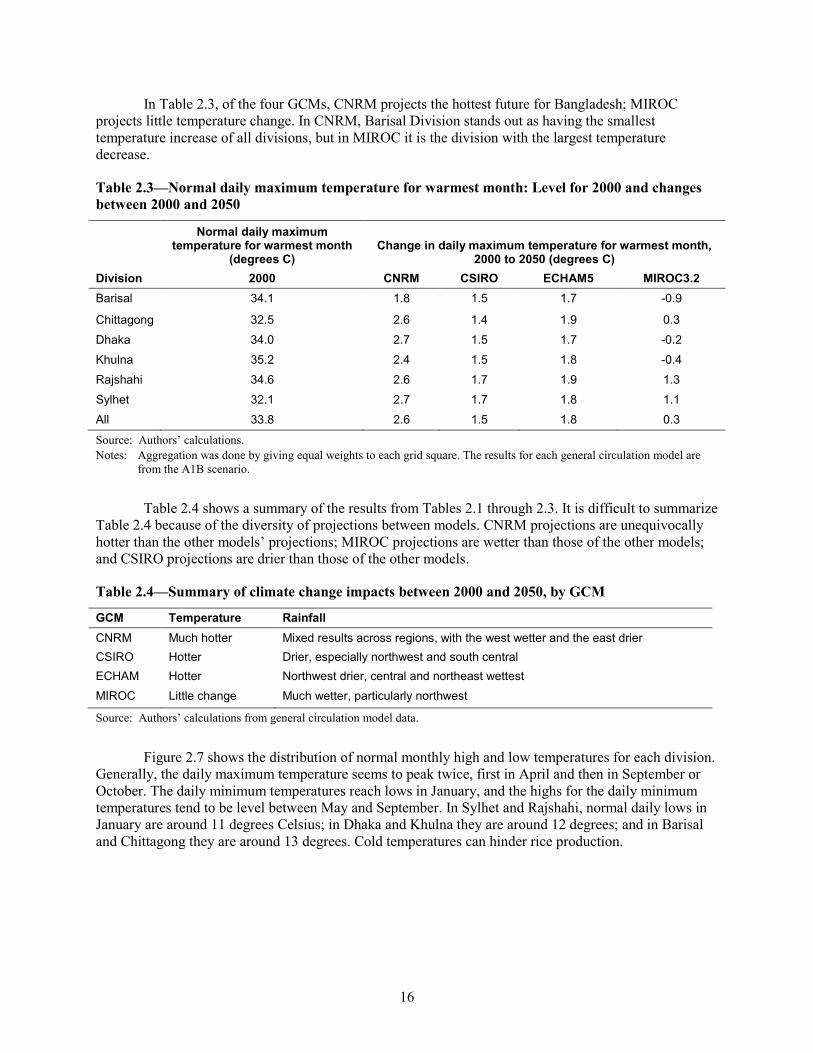
In Table 2.3, of the four GCMs, CNRM projects the hottest future for Bangladesh; MIROC projects little temperature change. In CNRM, Barisal Division stands out as having the smallest temperature increase of all divisions, but in MIROC it is the division with the largest temperature decrease.

Table 2.3—Normal daily maximum temperature for warmest month: Level for 2000 and changes between 2000 and 2050

Division

Normal daily maximum temperature for warmest month

(degrees C) Change in daily maximum temperature for warmest month,

2000 to 2050 (degrees C) 2000 CNRM CSIRO ECHAM5 MIROC3.2

Barisal 34.1 1.8 1.5 1.7 -0.9

Chittagong 32.5 2.6 1.4 1.9 0.3

Dhaka 34.0 2.7 1.5 1.7 -0.2

Khulna 35.2 2.4 1.5 1.8 -0.4

Rajshahi 34.6 2.6 1.7 1.9 1.3

Sylhet 32.1 2.7 1.7 1.8 1.1

All 33.8 2.6 1.5 1.8 0.3

Source: Authors’ calculations. Notes: Aggregation was done by giving equal weights to each grid square. The results for each general circulation model are

from the A1B scenario.

Table 2.4 shows a summary of the results from Tables 2.1 through 2.3. It is difficult to summarize Table 2.4 because of the diversity of projections between models. CNRM projections are unequivocally hotter than the other models’ projections; MIROC projections are wetter than those of the other models; and CSIRO projections are drier than those of the other models.

Table 2.4—Summary of climate change impacts between 2000 and 2050, by GCM

GCM Temperature Rainfall CNRM Much hotter Mixed results across regions, with the west wetter and the east drier CSIRO Hotter Drier, especially northwest and south central ECHAM Hotter Northwest drier, central and northeast wettest MIROC Little change Much wetter, particularly northwest

Source: Authors’ calculations from general circulation model data.

Figure 2.7 shows the distribution of normal monthly high and low temperatures for each division. Generally, the daily maximum temperature seems to peak twice, first in April and then in September or October. The daily minimum temperatures reach lows in January, and the highs for the daily minimum temperatures tend to be level between May and September. In Sylhet and Rajshahi, normal daily lows in January are around 11 degrees Celsius; in Dhaka and Khulna they are around 12 degrees; and in Barisal and Chittagong they are around 13 degrees. Cold temperatures can hinder rice production.

16

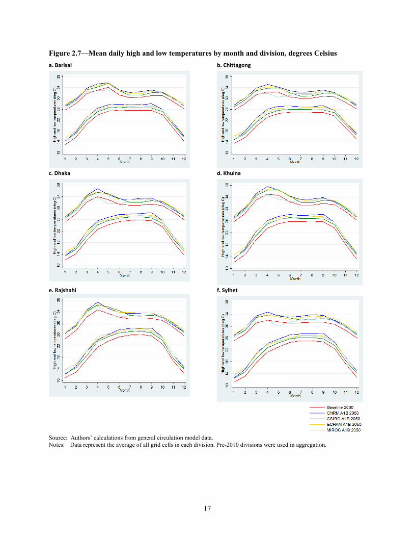
Figure 2.7—Mean daily high and low temperatures by month and division, degrees Celsius a. Barisal

b. Chittagong

c. Dhaka

d. Khulna

e. Rajshahi

f. Sylhet

Source: Authors’ calculations from general circulation model data. Notes: Data represent the average of all grid cells in each division. Pre-2010 divisions were used in aggregation.

17

Figure 2.8 shows the distribution of rainfall by division. As the rainfall map showed, the highest rainfall appears to be around Sylhet, followed closely by Chittagong. Khulna appears to have the lowest rainfall, followed closely by Rajshahi. Different divisions experience peak rainfall in different months. Sylhet and Dhaka appear to have their peak in June, while the other divisions appear to have it in July. Under some climate models, the peak month may shift. Khulna, Rajshahi, and Chittagong all have peak rainfall shifting from July to June in some of the GCMs.

Figure 2.8—Mean monthly precipitation by division, in millimeters a. Barisal

b. Chittagong

c. Dhaka

d. Khulna

e. Rajshahi

f. Sylhet


18

The months with the most rainy days roughly correspond to the peak rainfall months, though not perfectly. We note that in Sylhet, one of the GCMs suggests that the month with the most rainy days might shift from July to as early as May. In Khulna, one GCM suggests that the month with the most rainy days might shift forward, from July to August (Figure 2.9).

Figure 2.9—Mean monthly number of rainy days by division a. Barisal

b. Chittagong

c. Dhaka

d. Khulna

e. Rajshahi

f. Sylhet


19

Figure 2.10 shows the mean daily solar radiation for each month. All locations show two local maximums, with the greater of the two maximums in May and the smaller in September (except for Sylhet, where it is in August). In general, the higher the solar radiation, the faster crops will grow. GCMs disagree about whether solar radiation will rise in the future or fall.

Figure 2.10—Mean daily solar radiation by month and division, mJ/m2/day a. Barisal

b. Chittagong

c. Dhaka

d. Khulna

e. Rajshahi

f. Sylhet


20

DSSAT Results Figure 2.11 looks at the impact of climate change on production of rainfed aman rice for the four GCMs in our study, assuming the A1B climate scenario. The results shown compare the typical yield for the climate of 2000 with the typical yield for the climate of 2050. These yields were computed with the DSSAT crop modeling software, using an assumption of the application of 90 kg/ha of nitrogen (a “high” fertilizer application rate). The unit of analysis was a grid cell of 5 arc minutes, which is approximately 9 km square. In these particular results, we found the optimal planting month and optimal variety of rice (among 51 possible varieties available within DSSAT) in the year 2000, and then used the same month and variety in the 2050 climates projected by each GCM. We chose the planting month to be whatever gave the highest yields, within the June to August time frame. The results show changes in yield.

Figure 2.11—Change in yield of rainfed aman rice, high fertilizer levels, 2000 to 2050, with optimal planting date and variety for 2000 and the same date and variety used in 2050

a. CNRM

b. CSIRO

c. ECHAM

d. MIROC

Source: Authors’ calculations. Note: Scenario A1B.

21

There is some geographic variation within each GCM, as well as differences between GCMs. Generally, we note yield losses of between 2 and 10 percent, though all the models show some areas with yield losses between 10 and 20 percent as well as, much less frequently, areas with no significant change in yield or with increases of between 2 and 10 percent. While it is hard to compare the models accurately by visual inspection, it appears that the greatest losses are projected by the MIROC GCM and the smallest losses by the CNRM model, probably followed closely by the CSIRO model.

Figure 2.12 shows results of comparisons similar to those in Figure 2.11, but in this case the planting month and variety in 2050 were selected to be optimal under the new climate regime. We see smaller yield reductions and greater areas with yield gains compared with Figure 2.11. In particular, CNRM shows many areas of yield increases, covering much of the northern half of the country. We also note a much greater difference in model outcomes, with MIROC showing very few areas of projected yield increases, contrasting sharply with the CNRM model. Still, we see a lot of similarities between the CSIRO, ECHAM, and MIROC models, especially as we focus more on the central or core areas of the country.

Figure 2.12—Change in yield of rainfed aman rice, high fertilizer levels, 2000 to 2050, with optimal planting date and variety for both 2000 and 2050

a. CNRM

b. CSIRO

c. ECHAM

d. MIROC


22

Table 2.5 summarizes the results of the preceding figures, along with some additional results: Specifically, the result of “low” fertilizer application, at 10 kg/ha of nitrogen. Generally, we note that under low levels of fertilizer application, yields will tend to increase as a result of climate change, while under higher levels of fertilizer application, yields will tend to decrease as a result of climate change. This seems to imply that high-yield varieties are more sensitive to increased temperatures. It is important to note that higher fertilizer application still results in higher absolute yields, even when climate change is taken into consideration, so it will still be optimal (assuming prices of fertilizer do not rise too much) to use high levels of fertilizer rather than low levels of fertilizer.

Table 2.5—Changes in rainfed aman yields from 2000 to 2050, median change

Division

Low fertilizer High fertilizer

Keeping cultivar and planting month the

same as in 2000

Optimal cultivar and planting month for

2050


same as in 2000


2050 All 3.1% 5.8% -7.5% -4.0% Barisal -0.4% 1.8% -5.4% -3.8% Chittagong 1.7% 3.4% -7.6% -4.6% Dhaka 3.9% 6.0% -7.9% -4.4% Khulna -3.4% -1.2% -8.8% -6.7% Rajshahi 6.4% 9.8% -7.0% -2.3% Sylhet 6.1% 8.1% -7.1% -2.2% Source: Authors’ calculations.

Figure 2.13, similar to Figure 2.11, shows yield changes if rice variety and planting month for 2050 are fixed to the optimal levels of the year 2000. The planting month was again selected to give the highest yields—but within the November to February timeframe because we are considering irrigated boro rice. We note areas of yield gains in the southernmost part of the country as well as in the Chittagong hills, areas that do not currently have a large percentage of land planted in boro rice. However, we are aware that high soil and water salinity levels constrain boro rice in some of the southern districts in Bangladesh.

While there is agreement across models that these particular areas will be more favorable to boro rice in the future, the models disagree about changes for the rest of the country. The MIROC model projects that much of the central and western parts of the country will have no significant yield change; CNRM shows these same areas experiencing between 10 and 20 percent yield reduction with climate change.

23

Figure 2.13—Change in yield of irrigated boro rice, high fertilizer levels, 2000 to 2050, with optimal planting date and variety for 2000 and the same date and variety used in 2050

a. CNRM

b. CSIRO

c. ECHAM

d. MIROC


24

Figure 2.14 shows modeled results when allowing farmers to choose more optimal planting months and varieties for 2050 (we have always assumed the most optimal varieties for 2000). Changing planting dates and cultivars shows dramatic improvements in boro yield even under climate change. The greatest yield increases are found in the ECHAM model: Very few areas show declining yields, and some areas show yield increases of greater than 20 percent, with the majority of the country showing yield increases between 10 and 20 percent. The results for CNRM are much more pessimistic: Much of the northwest portion of the country shows yield losses between 2 and 10 percent, and some areas show losses between 10 and 20 percent. CSIRO results are similar to those of the CNRM model, while the MIROC results are similar to those of the ECHAM model.

Figure 2.14—Change in yield of irrigated boro rice, high fertilizer levels, 2000 to 2050, with optimal planting date and variety for both 2000 and 2050

a. CNRM

b. CSIRO

c. ECHAM

d. MIROC


25

Further analysis shows that most of the yield gains between the restricted model of Figure 2.13 and the less restricted model of Figure 2.14 are due to changes in planting month. The temperature profiles of Figure 2.7 show minimum temperatures that are too low for good rice growth under the climate of 2000. The rise of a few degrees by 2050 allows the planting month to shift from January or February to November or December, allowing the rice to avoid the high temperatures of April and May. Sattar (2000) confirmed the impeding effect of the cold on boro rice in Bangladesh. Moving the planting date to November would impact the aman harvest, because aman must be harvested before boro is planted. Furthermore, the optimal cultivar to plant for aman, taking into consideration climate change, is a longer-duration variety than the one used in the baseline 2000 climate; its use would conflict with boro planting, especially if the boro planting is done earlier. These conflicts point to the need for more research into optimal crop rotations as well as other aspects of farming systems.

Table 2.6 summarizes the results for irrigated boro rice. Contrary to the results for rainfed aman rice, yield losses under climate change are higher for low fertilizer usage than for high fertilizer usage. Similarly, changing the planting month and rice variety produces very little gain in yield at the low fertilizer level but a very large gain at the high fertilizer level.

Table 2.6—Changes in irrigated boro yields from 2000 to 2050, median change

Division

Low fertilizer High fertilizer


same as in 2000


2050


same as in 2000


2050 All -9.2% -8.9% -6.6% 3.6% Barisal -10.7% -10.2% 1.9% 11.3% Chittagong -6.9% -6.3% -2.9% 7.7% Dhaka -9.0% -8.9% -8.0% 4.6% Khulna -10.5% -10.1% -8.0% 1.8% Rajshahi -8.0% -7.7% -7.5% 0.3% Sylhet -12.4% -11.4% -7.5% 2.2% Source: Authors’ calculations.

Note that the column “Keeping cultivar and planting month the same as in 2000” represents the results we might expect if farmers do not adapt to climate change or adapt slowly. The column “Optimal cultivar and planting month for 2050” shows results when farmers adapt, as would more likely be the case if there were active linkages between research, extension, and farmers. The difference between these two columns—when converted to monetary units for each crop—may provide a measure of value for research and extension under climate change. We see that if farmers do not adapt to climate change, under the high-fertilizer scenario, boro yields will decline by 6.6 percent, while if they do adapt, yields will actually increase by 3.6 percent. That gap, between adaptation and no adaptation, is therefore 10.2 percent of current boro production. For aman, the value is 3.5 percent of current production.

Table 2.7 summarizes the main results for all crops analyzed with DSSAT for yield impacts of climate change. We considered the impacts at two levels of fertilizer use. The low level was set at 10 kg/ha of nitrogen; the higher level differed between crops, since what would be a reasonable high for a non-nitrogen-fixing crop like rice would be too high for a nitrogen-fixing crop like soybeans. Table 2.8 shows the levels of nitrogen used for the high-fertilizer experiments for each crop, along with yield response from fertilizer use.

26

Table 2.7—Changes in crop yields from 2000 to 2050, median value from all four GCMs

Crop

Low fertilizer High fertilizer Keeping cultivar

and planting month the same as

in 2000

Optimal cultivar and planting

month for 2050

Keeping cultivar and planting

month the same as in 2000

Optimal cultivar and planting

month for 2050 Rainfed rice (aman) 3.1% 5.8% -7.5% -4.0%

Irrigated rice (boro) -9.2% -8.9% -6.6% 3.6%

Rainfed wheat -20.4% -16.4% -18.7% -15.5%

Irrigated wheat -10.8% -10.8% -20.4% -20.4%

Rainfed maize 2.4% 4.1% -2.8% -2.1%

Irrigated maize 2.1% 4.0% -1.4% -0.8%

Rainfed sugarcane -10.6% -10.4% -10.6% -10.4%

Rainfed soybeans -9.3% -9.0% -9.5% -9.5%

Rainfed groundnuts -13.5% -10.9% -13.5% -10.7%

Rainfed sorghum -8.5% -7.5% -8.8% -7.8%

Rainfed taro 0.3% 1.4% -10.2% -7.3%

Irrigated taro -10.7% -8.0% -8.4% -7.3%

Source: Authors’ calculations. Notes: Irrigated groundnuts, sugarcane, soybeans, and sorghum had yields similar to their rainfed counterparts and were

therefore omitted from this table. The sugarcane crop model does not have a fertilizer response. Aggregation was done by taking a weighted average of cropland in each square.

Wheat is also a significant crop for Bangladesh, and the impact of climate change on wheat is predicted to be severe, approaching 20 percent of yield. The impact on sugarcane, soybeans, and groundnuts is also quite high, at around 10 percent. The impact of climate change on maize, however, might be positive (under low fertilizer) and would likely be only slightly negative even under high fertilizer use.

Of course, these results do not take into account future varieties that may be developed to be resistant to heat or other stresses such as cold, drought, or floods. The IMPACT model (discussed below) attempts to project such technological developments.

Table 2.8 shows that for many crops, losses in yield due to climate change can be compensated for by increasing the availability of nitrogen in the soil. Fertilizer effectiveness under climate change will fall for many crops: for aman, the rate of yield increase drops from 11.0 percent to 8.9 percent for each additional 10 kg/ha of nitrogen. It is nevertheless effective for improving yields. In some cases, the effectiveness of fertilizer actually rises: For boro rice, the rate of yield increase improves, from 9.7 percent to 12.6 percent, for each additional 10 kg/ha of nitrogen. Nitrogen can be added to the soil using chemical fertilizers, but it can also be done, at least in part, through better soil fertility management, including the use of animal manure, cover crops, crop rotations, and crop or agroforestry residue.

27

Table 2.8—Yield response from supplementing nitrogen in the soil

Crop

Nitrogen used for high-fertilizer scenarios

(kg N / ha)

% change in yield for each additional 10 kg N / ha

2000 2050 Rainfed rice (aman) 90 11.0% 8.9%

Irrigated rice (boro) 90 9.7% 12.6%

Rainfed wheat 60 1.6% 0.9%

Irrigated wheat 60 5.3% 2.6%

Rainfed maize 90 8.1% 6.8%

Irrigated maize 90 10.0% 9.1%

Rainfed soybeans 60 -0.2% -0.3%

Rainfed groundnuts 30 -0.1% 0.0%

Rainfed taro 90 10.2% 8.1%

Irrigated taro 90 6.2% 6.4%

Source: Authors’ calculations. Notes: N = nitrogen.

Irrigated groundnuts, sugarcane, soybeans, and sorghum had similar yields to their rainfed counterparts and were therefore omitted from this table. The sugarcane crop model does not have a fertilizer response, and the soybean fertilizer response was not measured. Aggregation was done by taking a weighted average of cropland in each square.

The value for 2050 shows the median value of the results for the four general circulation models using optimal month and cultivar.

Table 2.9 shows the areas cultivated for major crops in Bangladesh, along with average yields for those crops. We see the importance of both aman and boro rice; boro area is less than aman area, but higher yields result in higher total rice production for boro. Jute, wheat, potatoes, maize, and sugarcane are also very important crops.

Table 2.9—Harvest area and production of major crops in Bangladesh

Crop Area harvested

(ha) Production

(MT) Yield

(MT/ha) Rice, aman 5,231,587 10,300,000 2.0

Rice, boro 4,432,752 16,400,000 3.7

Rice, aus 912,317 1,509,589 1.7

Jute 429,537 862,383 2.0

Wheat 393,814 790,519 2.0

Potatoes 373,382 5,907,225 15.8

Maize 157,153 922,370 5.9

Sugarcane 143,978 5,421,511 37.7

Source: BBS 2008. Notes: Two-year averages for wheat, rice, jute, and potatoes (2006/07 and 2007/08). Three-year averages for sugarcane and

maize (2006/07 and 2007/08).

The tables show potential gains from optimal farm management, as well as potential losses from climate change without adaptation. The pace of climate change in the next 40 years is likely to be faster than indigenous methodologies can adapt—faster, that is, than traditional learning and communication can take place between farmers and between generations. Small farmers will suffer adverse effects of

28

climate change unless agricultural research and extension can develop successful cultivars as well as complementary farming practices, and pass the research results on to farmers. In order for Bangladesh to succeed and thrive, investment must be increased in research and extension institutions, while the institutions must focus on helping the small farmer succeed amid the changes and uncertainty concerning the future environment.

IMPACT Model Findings For alternative projections, we draw on the results of IFPRI’s IMPACT (International Model for Policy Analysis of Agricultural Commodities and Trade) model. While the crop model results are probably the most informative results regarding the direct effect of climate change on agricultural production, the IMPACT results are useful because they take into account changes in food trade as a result of climate change as well as assumptions about technological change, even while controlling for climate impacts on productivity. Nelson, Rosegrant, Palazzo, et al. (2010) used the IMPACT model to study the impact of climate change on global agriculture and food consumption. This section focuses on the most important results for Bangladesh. First, however, it will be helpful to give a brief description of the model.

The IMPACT model was initially developed at the International Food Policy Research Institute (IFPRI) to project global food supply, food demand, and food security to year 2020 and beyond (Rosegrant et al. 2008). It is a partial equilibrium agricultural model with 32 crop and livestock commodities, including cereals, soybeans, roots and tubers, meats, milk, eggs, oilseeds, oilcakes and meals, sugar, and fruits and vegetables. IMPACT has 115 country (or in a few cases country-aggregate) regions, with specified supply, demand, and prices for agricultural commodities. Large countries are further divided into major river basins. The result is 281 spatial units called food production units. The model links the various countries and regions through international trade, using a series of linear and nonlinear equations to approximate the underlying production and demand relationships. World agricultural commodity prices are determined annually at levels that clear international markets. Growth in crop production in each country is determined by crop and input prices, exogenous rates of productivity growth and area expansion, investment in irrigation, and water availability. Demand is a function of prices, income, and population growth. Climate change effects on crop production enter into the IMPACT model by altering both crop area and yield (Nelson, Rosegrant, Palazzo et al. 2010).

Nelson, Rosegrant, Palazzo, et al. (2010) posed three scenarios or projections of population and gross domestic product (GDP) per capita. The optimistic scenario assumes high GDP per capita growth and low population growth in each country of the world; the pessimistic scenario assumes low GDP per capita growth and high population growth in each country of the world; and the baseline or median scenario assumes levels of GDP per capita growth and population growth between those of the two other scenarios. Because we choose to focus on the impact of climate change, we use the median GDP per capita and population scenarios to consider the impact of climate change on each of the areas studied. Also, by focusing on just one scenario of GDP per capita alongside climate change, we avoid one of the pitfalls that arises from trying to derive national-level policy implications from a global-level analysis: the implied assumption that, if one nation’s GDP increases, the GDP for every nation increases. This assumption makes it difficult to analyze the implications of one nation’s increasing (or decreasing) its GDP while that of all the other nations remains the same.

Nelson, Rosegrant, Palazzo, et al. (2010) chose to include five scenarios pertaining to climate. They used the CSIRO GCM, under both the B1 and A1B climate scenarios; the MIROC GCM, under both the B1 and A1B climate scenarios; and a fifth analysis, assuming no change in climate.

Future Income and Population Figure 2.15 shows the projected GDP per capita assumed in the IMPACT analysis, which is based on GDP assumptions from the World Bank study Economic Analysis of Climate Change (World Bank 2010b), along with the medium variant of the United Nations’ Population Department population projections (UNPop 2009). In this graph, we see that GDP per capita in Bangladesh is projected by 2050

29

to increase to five times the level of 2010; most of the change takes place in the last half of that period, after doubling between 2010 and 2030.

Figure 2.15—Projected GDP per capita

Source: Computed from GDP (gross domestic product) data from the World Bank Economic Adaptation to Climate Change

project (World Bank 2010b), from the Millennium Ecosystem Assessment (2005) reports, and from population data from the United Nations (UNPop 2009).

Figure 2.16 shows population projections from the United Nations (UNPop 2009). Focusing on the medium variant, we note that population is projected to increase from nearly 165 million in 2010 to just over 220 million in 2050, a 0.7 percent annual growth rate over the entire period. In this case the upward curve levels off, from almost 1 percent annual growth over the first 20 years, to less than 0.5 percent annual growth over the second 20 years.

Figure 2.16—Projected population

Source: UNPop 2009.

30

World Prices Figure 2.17 shows food prices between 2010 and 2050 as projected by IMPACT for some important food commodities. These are summarized in Table 2.10 for the years 2000 and 2050. The five scenarios show a fairly consistent ranking, from highest to lowest price projections: MIROC A1B, MIROC B1, CSIRO A1B, CSIRO B1, and no climate change—though this pattern does not hold for all crops (for example, sweetpotatoes and yams).

Figure 2.17—Food price projections.

31

Figure 2.17—Continued

Source: Nelson, Rosegrant, Palazzo, et al. 2010.

Of the three main staples in the world—rice, wheat, and maize—we see that rice prices increase the least, while maize prices increase by more than twice the percentage increase for rice. Under MIROC A1B, rice increases by 83 percent while maize increases by 209 percent. This may suggest future advantages from switching from rice cultivation to maize cultivation in some parts of Bangladesh that could climatically support such a change.

32

National Production and Consumption Figure 2.18 shows the IMPACT model predictions for the number of undernourished children in Bangladesh. Under all circumstances, the number of undernourished children under five years old is projected to drop.

Figure 2.18—Malnutrition projections for children under five years of age


In Figure 2.19, we see that rice yields are predicted to rise, increasing by 24 percent between 2010 and 2050. Figure 2.20 shows rice-growing areas rising slightly between 2010 and 2025, and falling slightly through 2050. The yield gains outweigh the area losses, in terms of impact on production, until around 2045, with production falling in some of the models very slightly after that (Figure 2.21). Rising production without corresponding increased domestic demand for rice (and a projected drop in per capita rice consumption) leads to increasing rice exports between 2010 and 2050 (Figure 2.22).

Figure 2.19—Yield projections for rice


33

Figure 2.20—Harvest area projections for rice


Figure 2.21—Production projections for rice


34

Figure 2.22—Net export projections for rice


While we present the results only for rice, the IMPACT model has results for all of the items listed in Table 2.10, as well as a few others that are of lesser importance for Bangladesh and were thus omitted from the table.

Table 2.10—Percent changes in world prices of food commodities, 2000 to 2050

Crop

MIROC CSIRO No climate change

A1B B1 A1B B1 Rice 83% 87% 85% 82% 54%

Wheat 121% 106% 99% 93% 66% Maize 209% 165% 156% 145% 103% Potatoes 37% 28% 43% 46% 0% Sweetpotatoes & yams 141% 96% 156% 120% 60% Cassava 78% 50% 64% 42% 18% Sugarcane 125% 113% 108% 103% 77% Sorghum 115% 104% 110% 104% 82% Millet 8% 8% 14% 13% 8% Other grains 102% 84% 89% 81% 47% Soybeans 120% 100% 75% 64% 48% Chickpeas 17% 22% 35% 31% 22% Pigeon peas -7% -6% 6% 4% -1% Groundnuts 35% 33% 37% 33% 13% Beef 59% 58% 57% 57% 54% Pork 56% 54% 53% 53% 50% Lamb 35% 34% 34% 34% 33% Poultry 61% 58% 58% 57% 53% Eggs 32% 30% 30% 29% 27% Milk -10% -11% -11% -11% -12%


35

3. HOUSEHOLD SURVEY

As part of this study, we designed and conducted a survey of agricultural households in order to provide background information on landownership, size of operation, rice production, input use, and farm practices in rural communities, as well as to identify and assess existing climate change adaptation strategies. A household was considered to be involved in agriculture if it (a) was operating cultivated land (either owned, leased, shared, or mortgaged), or (b) owned 5 or more livestock, or (c) raised 50 or more poultry. The household survey covered 40 unions (administrative units), selected to represent the 7 broad agroecological zones (AEZs) as grouped by the Bangladesh Centre for Advanced Studies, based on the 30 AEZs identified by the Soil Resources Development Institute (SRDI) (Table 3.1). The seven AEZs are Barind Tract, tidal floodplains, Modhupur tract, Himalayan piedmont plain, beel and haor basins, northern and eastern hills, and floodplains.

Table 3.1—SRDI’s 30 agroecological zones, grouped into 7 agroecological zones.

New Agroecological Zone SRDI Agroecological Zone

Barind Tract Level Barind Tract Northeastern Barind Tract High Barind Tract

Beel and haor basin

Sylhet Basin Eastern Surma–Kusiyara Floodplain Lower Atrai Basin Arial Beel Gopolganj–Khulna Beels

Floodplain

Tista Meander floodplain Active Tista Floodplain Active Brahmaputra–Jamuna Floodplain Young Brahmaputra–Jamuna Floodplain Old Brahmaputra Floodplain Lower Punarbhaba Floodplain Karatoya–Bangali Floodplain High Ganges River Floodplain Active Ganges Floodplain Old Meghna Estuarine Floodplain Low Ganges River Floodplain Middle Meghna River Floodplain Lower Meghna River Floodplain

Himalayan Piedmont Plain Old Himalayan Piedmont Plain Northern and Eastern Piedmont Plain

Modhupur Tract Modhupur Tract

Northern and eastern hills Northern and Eastern Hills Akhaura Terrace

Tidal floodplain

Chittagong Coastal Plain Ganges Tidal Floodplain Young Meghna Estuarine Floodplain St. Martin’Coral Island

Source: Authors.

36

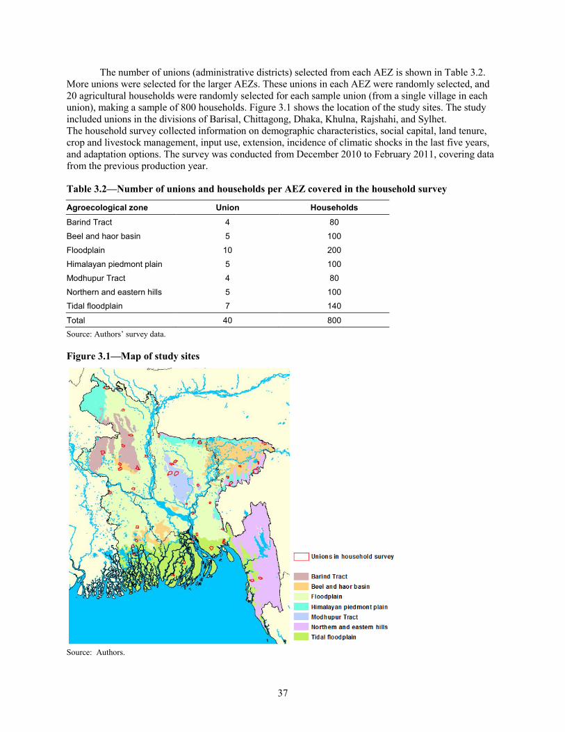
The number of unions (administrative districts) selected from each AEZ is shown in Table 3.2. More unions were selected for the larger AEZs. These unions in each AEZ were randomly selected, and 20 agricultural households were randomly selected for each sample union (from a single village in each union), making a sample of 800 households. Figure 3.1 shows the location of the study sites. The study included unions in the divisions of Barisal, Chittagong, Dhaka, Khulna, Rajshahi, and Sylhet. The household survey collected information on demographic characteristics, social capital, land tenure, crop and livestock management, input use, extension, incidence of climatic shocks in the last five years, and adaptation options. The survey was conducted from December 2010 to February 2011, covering data from the previous production year.

Table 3.2—Number of unions and households per AEZ covered in the household survey

Agroecological zone Union Households

Barind Tract 4 80

Beel and haor basin 5 100

Floodplain 10 200

Himalayan piedmont plain 5 100

Modhupur Tract 4 80

Northern and eastern hills 5 100

Tidal floodplain 7 140

Total 40 800 Source: Authors’ survey data.

Figure 3.1—Map of study sites

Source: Authors.

37

Brief Profile of Sample Households About 94 percent of the households in our sample were headed by males (Table 3.3). The highest percentage of male-headed households was found in the beel and haor basin AEZ (99 percent), followed by the northern and eastern hills AEZ (98 percent). The highest number of female-headed households was found in the Modhupur Tract (19 percent).

Table 3.3—Percentage distribution of gender of household head, by AEZ

Agroecological zone

Gender (%) Total (%)

Male Female

Barind Tract 95 5 100

Beel and haor basin 99 1 100

Floodplain 94 7 100

Himalayan piedmont plain 95 5 100

Modhupur Tract 81 19 100

Northern and eastern hills 98 2 100

Tidal floodplain 96 4 100

All AEZs 94 6 100 Source: Authors’ survey data.

The majority of household heads in all AEZs were married (Table 3.4). The highest percentage of married household heads was found in the tidal floodplain (97 percent) and the lowest percentage in the beel and haor basin (90 percent), while the Himalayan Plain had the highest percentage for widowed household heads (5 percent). Only in the Modhupur Tract were divorced and separated household heads observed.

Table 3.4—Percentage distribution of marital status of household head, by AEZ

Agroecological zone

Marital status (%) Total (%) Unmarried Married Widowed Divorced Separated

Barind Tract 1 96 3 0 0 100

Beel and haor basin 7 90 3 0 0 100

Floodplain 3 95 2 0 0 100

Himalayan piedmont plain 3 92 5 0 0 100

Modhupur Tract 1 93 4 1 1 100

Northern and eastern hills 4 93 3 0 0 100

Tidal floodplain 1 97 1 0 0 100

All AEZs 3 94 3 0 0 100 Source: Authors’ survey data.

The average household was composed of 5.0 members (Table 3.5). This is slightly bigger than the national average of 4.5 members (Bangladesh, Bureau of Statistics 2010). Based on the survey, mean household size was highest in the northern and eastern hills (6.2 members) and lowest in the Barind Tract (3.9 members).

38

Table 3.5—Mean household size, and mean age and years of schooling of household head, by AEZ

Agroecological zone Household size Age Years of schooling

Barind Tract 3.9 45.6 3.5

Beel and haor basin 5.1 45.9 3.8

Floodplain 4.7 44.4 3.7

Himalayan piedmont plain 4.9 44.5 4.9

Modhupur Tract 4.7 45.7 3.1

Northern and eastern hills 6.2 47.1 2.3

Tidal floodplain 5.3 46.4 3.3

All AEZs 5.0 45.5 3.5 Source: Authors’ survey data.

The mean age of household heads in all AEZs was 45.5 years (Table 3.5). The highest average age of household heads was in the northern and eastern hills, at 47.1 years; the lowest was in the floodplain, at 44.4 years.

Education of household heads was fairly low (Table 3.5), with 3.5 years of schooling on average; the highest level was found in the Himalayan piedmont plain (4.9 years) and the lowest in the northern and eastern hills (2.3 years). Table 3.6 shows that almost half of farm household heads (47 percent) did not have any education. The percentage with no education was highest in the northern and eastern hills (57 percent) and lowest in the Himalayan Plain (31 percent). The Himalayan Plain also had the highest percentage of household heads with a Bachelor of Arts or Bachelor of Science degree (5 percent). Only the Barind Tract, the floodplain, and the tidal floodplain had household heads with a Master of Arts or Master of Science degree.

Table 3.6—Highest class passed by household head (percent)

Education (highest class passed)

Barind Tract

Beel and haor basin

Floodplain

Himalayan Plain

Modhupur Tract

Northern and

eastern hills

Tidal flood-plain

All AEZs

No education 51 43 49 31 50 57 49 47 Completed class 1 3 1 1 3 3 6 1 2 Completed class 2 - 5 5

1 7 5 4

Completed class 3 1 2 1 7 8 1 3 3 Completed class 4 6 4 7 7 5 7 4 6 Completed class 5 6 10 10 10 10 7 11 9 Completed class 6 5 6 2 2 1 3 4 3 Completed class 7 1 5 4 10 1 2 6 4 Completed class 8 5 6 3 6 9 1 3 4 Completed class 9 15 11 6 10 4 2 4 7 Completed secondary school 4 5 7 7 6 3 6 6 Completed higher secondary 1 2 4 2 1 3 1 2 Bachelor’s degree - - 2 5 1 1 2 2 Master’s degree 1 - 2 - - - 1 1 Total 100 100 100 100 100 100 100 100

Source: Authors’ survey data.

39

Landownership and Farm Operation Of the 800 agricultural households surveyed, 252 were landless (Table 3.7), but only 6 were not operating agricultural land. The rest of the landless were either renting agricultural land (or using shared or mortgaged land) or held temporary user right for the land they were operating.5 For the 252 landless households who were operating land, the most common farm size was 0.2–0.4 ha (75 farmers). Only 10 of these households farmed more than 1 ha.

Table 3.7—Households’ owned land size class versus operated land size class (number of households)

Owned land size class (ha)

Operated land size class (ha) Total

None < 0.1 0.1–0.2 0.2–0.4 0.4–0.7 0.7–1.0 > 1.0 None 6 30 54 75 54 23 10 252 < 0.1 1 50 17 24 16 5 2 112 0.1–0.2 1 9 63 18 13 5 1 110 0.2–0.4 3 4 12 78 16 9 3 125 0.4–0.7 2 3 3 8 68 5 9 98 0.7–1.0 3 0 3 1 7 23 10 47 > 1.0 1 0 4 2 5 3 41 56 Total 17 96 153 206 179 73 76 800


Of the 800 agricultural households surveyed, only 16 were not cultivating land but were involved in livestock raising or fish farming, or both. Out of the 206 farmers who operated a farm ranging from 0.2 to 0.4 ha, 78 owned agricultural land in the same range.

Owned agricultural lands were relatively small in all AEZs, averaging only 0.21 ha (Table 3.8). Owned farms in the floodplain had the smallest area (0.15 ha), followed by the tidal floodplain (0.19 ha). The Barind Tract registered the largest owned farm size, averaging 0.28 ha, followed by the Himalayan Plain (0.25 ha) and the beel and haor basin (0.23 ha). Across all AEZs, the average number of plots per owned farm was 2.07, ranging from 1.41 (tidal floodplain) to 2.73 (Barind Tract).

Table 3.8—Households’ average farm size and number of plots, by AEZ

Agroecological zone

Owned size (ha)

Operated size (ha) Plots owned Plots operated Number of

observations

Barind Tract 0.28 0.35 2.73 3.43 80

Beel and haor basin 0.23 0.38 2.21 3.92 100

Floodplain 0.15 0.22 2.04 2.87 200

Himalayan Plain 0.25 0.34 2.31 3.04 100

Modhupur Tract 0.20 0.29 2.55 3.44 80 Northern and eastern hills 0.21 0.41 1.80 3.43 100

Tidal floodplain 0.19 0.34 1.41 2.52 140

All AEZs 0.21 0.32 2.07 3.14 800 Source: Authors’ survey data.

5 Temporary user right refers to a situation wherein land is allowed to be used for free, without any rent, usually between family members. The person can cultivate the land but cannot sell it, and must stop using the land when the owner asks for it.

40

The average operated size of farms in all AEZs (0.32 ha) exceeded the average owned farm size, indicating that the farmers were renting additional agricultural lands. Farmers in the northern and eastern hills had the largest average operated farm size (0.41 ha), almost double their average owned farm size. The floodplain had the smallest operated farm size (0.22 ha).

Farms consist of one or more plots, and the plots belonging to a single farm are not generally located together (meaning not adjacent). The average number of plots per operated farm was 3.14, ranging from 2.52 (tidal floodplain) to 3.92 (beel and haor basin).

Rice Cultivation

Plot Size Table 3.9 shows the average rice plot size per farm household, by AEZ and growing season. During the aus and boro seasons, farm households in the Barind Tract operated the largest rice plot size (0.74 ha and 0.81 ha, respectively); in aman season, farm households in the beel and haor basin operated the biggest rice plot size. Except for the Barind Tract and the northern and eastern hills, farmers operated smaller rice plots during the aus season, on average, and bigger rice plots during the aman and boro seasons. In the Barind Tract, farmers operated larger rice plots during the boro and aus seasons and a smaller rice plot during the aman season (0.46 ha). In the northern and eastern hills, farmers operated larger rice plots during the aman season (0.58 ha), decreasing to 0.47 ha in the aus season and to 0.22 ha in the boro season. Overall, the average rice plot size was bigger during the boro season (0.44 ha) and the aman season (0.43 ha). It was smaller during the aus season (0.37 ha).

Table 3.9—Average household rice plot size by AEZ

Agroecological zone

Aus Aman Boro

n Size (ha) n

Size (ha) n

Size (ha)

Barind Tract 18 0.74 72 0.46 80 0.81

Beel and haor basin 6 0.14 29 0.59 74 0.64

Floodplain 71 0.21 159 0.24 158 0.23

Himalayan Plain 17 0.32 94 0.48 74 0.45

Modhupur Tract 1 0.26 52 0.34 61 0.32 Northern and eastern hills 53 0.47 88 0.58 28 0.22

Tidal floodplain 37 0.39 109 0.51 38 0.43

All AEZs 203 0.37 603 0.43 513 0.44 Source: Authors’ survey data.

Planting Date The most common planting month during the aus season was May (47.16 percent of plots), followed by April (28.18 percent of plots) (Table 3.10). For aman season, the most common planting month was July (40.32 percent), followed by August (36.81 percent). For boro season, the most common planting month was January (60.37 percent of plots).

41

Table 3.10—Planting date for each type of rice (plot level)

Planted month

Aus Aman Boro Frequency % Frequency % Frequency %

January 5 0.98 10 0.62 780 60.37 February 1 0.2 3 0.18 212 16.41 March 35 6.85 1 0.06 28 2.17 April 144 28.18 13 0.8 7 0.54 May 241 47.16 28 1.73 4 0.31 June 56 10.96 143 8.82 2 0.15 July 19 3.72 654 40.32 7 0.54 August 3 0.59 597 36.81 5 0.39 September 7 1.37 166 10.23 0 0 October 0 0 2 0.12 1 0.08 November 0 0 1 0.06 22 1.7 December 0 0 4 0.25 224 17.34 Total plots 511 100 1,622 100 1,292 100


Fertilizer and Pesticide Use Table 3.11 shows that, on average, the smallest rice farms (less than 0.1 ha) had the highest application of nitrogen (N), phosphorus (P), and potassium (K) fertilizers, at 97.31, 25.09, and 23.72 kg/ha, respectively. Rice farms in the biggest land size class (more than 1.0 ha) had the lowest application of N and P fertilizers, at an average of 59.64 kg/ha and 14.23 kg/ha, respectively.

Table 3.11—Households’ fertilizer use by operated land size class (for rice only)

Operated land size class (ha) Number of observations N

kg/ha K

P < 0.1 78 97.31 25.09 23.72 0.1–0.2 150 83.75 24.46 21.86 0.2–0.4 204 81.13 20.97 19.05 0.4–0.7 178 78.71 20.31 19.60 0.7–1.0 72 87.63 17.76 16.60 > 1.0 75 59.64 14.23 16.96 Total/average 757 81.24 20.96 19.78

Source: Authors’ survey data. Notes: N = nitrogen; P = phosphorus; K = potassium.

Table 3.12 compares fertilizer use in rice cultivation AEZs. On average, farm households in the floodplain exhibited the highest rate of N fertilizer application (103.94 kg/ha). Farm households in northern and eastern hills applied the lowest average rate of N fertilizer use (44.78 kg/ha).

42

Table 3.12—Households’ fertilizer use by AEZ (for rice only)

Agroecological zone Number of

observations N kg/ha

K P

Barind Tract 80 95.06 29.86 34.07

Beel and haor basin 93 84.89 17.88 22.49

Floodplain 195 103.94 26.46 26.08

Himalayan piedmont plain 100 85.23 19.01 18.39

Modhupur Tract 67 78.39 24.20 17.27

Northern and eastern hills 96 44.78 13.34 10.09

Tidal floodplain 126 60.74 14.69 8.76

All AEZs 757 81.24 20.96 19.78

Source: Authors’ survey data. Notes: N = nitrogen; P = phosphorus; K = potassium.

The Barind Tract had the highest rate of P (29.86 kg/ha) and K fertilizers (34.07 kg/ha), followed by the floodplain (26.46 kg/ha and 26.08 kg/ha, respectively) and Modhupur tract (24.20 kg/ha and 22.49 kg/ha, respectively). The northern and eastern hills had the lowest average rate of P and K fertilizer use (13.34 kg/ha and 10.09 kg/ha, respectively), followed by the tidal floodplain (14.69 kg/ha and 8.76 kg/ha, respectively). Overall, the average rates of N, P, and K fertilizer application for rice production were 81.24, 20.96, and 19.78 kg/ha, respectively.

Table 3.13 shows that the mean pesticide use for rice production was higher for smaller farms than bigger farms. The smallest farm size class (less than 0.1 ha) had the highest mean pesticide use (2,334.51 taka/ha) while the largest (more than 1 ha) had the lowest pesticide application (1,276.49 taka/ha). Mean pesticide use was 1,680.15 taka/ha.

Table 3.13—Households’ pesticide use (rice only) by operated land size class

Operated land size class (ha)

Number of observations

Pesticide use (taka/ha)

< 0.1 78 2,334.51 0.1–0.2 150 1,946.64 0.2–0.4 204 1,516.93 0.4–0.7 178 1,601.10 0.7–1.0 72 1,494.45 > 1.0 75 1,276.49 Total 757 1,680.15


Among the seven AEZs, pesticide use was highest among farm households in the Barind Tract (Table 3.14). The Modhupur Tract had the lowest mean pesticide use (1,116.60 taka/ha), followed by the Himalayan Plain (1,148.55 taka/ha) and the northern and eastern hills (1,284.28 taka/ha).

43

Table 3.14—Households’ pesticide use (rice only) by AEZ

Agroecological zone Number of

observations Pesticide use

(taka/ha)

Barind Tract 80 2,536.74

Beel and haor basin 93 1,740.87

Floodplain 195 1,819.45

Himalayan Plain 100 1,148.55

Modhupur Tract 67 1,116.60

Northern and eastern hills 96 1,284.28

Tidal floodplain 126 1,899.08

All AEZs 757 1,680.15 Source: Authors’ survey data.

Rice Yield Mean rice yield showed a decreasing trend as the operated land size increased, except for farms of 0.10–0.199 ha (Table 3.15). Farms of less than 0.1 ha showed the highest mean rice yield (4,650.05 kg/ha) due their higher fertilizer and pesticide usage. Moreover, farms in Bangladesh are generally labor intensive, and smaller farms are even more so. Farms of more than 1 ha had the lowest mean rice yield (3,557.05 kg/ha). The mean rice yield of all the 757 sample respondents was 4,133.54 kg/ha.

Table 3.15—Rice yield by operated land size class


Number of observations

Rice yield (kg/ha)

< 0.1 78 4,650.05 0.1–0.2 150 4,157.79 0.2–0.4 204 4,324.65 0.4–0.7 178 4,114.05 0.7–1.0 72 3,630.72 > 1.0 75 3,557.05 Total 757 4,133.54


Losses in Rice Production Paddy loss showed an increasing trend as the operated land size increased (Table 3.16). The smallest land size class (less than 0.1 ha) incurred the lowest paddy loss (9.7 percent), while farms of more than 1 ha showed the highest paddy loss (20.71 percent). The lower dosage of pesticides might partly account for the higher paddy loss in the larger farms.

44

Table 3.16—Households’ rice paddy loss by operated land size class (loss in percent)


Number of observations Loss (%)

< 0.1 78 9.70 0.1–0.2 150 12.47 0.2–0.4 204 13.75 0.4–0.7 178 14.43 0.7–1.0 72 18.14 > 1.0 75 20.71 Total 757 14.35

Source: Authors’ survey data. Note: Percentage of loss is calculated by the following formula: Loss (%) = loss quantity/(harvested + quantity in field + loss quantity) * 100.

Table 3.17 shows the distribution of rice loss by reason and by AEZ. Insects, rodents, and viruses caused the highest proportion of rice losses in the Barind Tract (42 percent), Modhupur Tract (47 percent), and northern and eastern hills (58 percent). Floods, waterlogging, and river erosion caused a high proportion of losses in the beel and haor basin, Himalayan Plain, Barind Tract, and tidal floodplain (81 percent, 34 percent, 35 percent, and 35 percent, respectively). Rice losses in the floodplain were largely due to drought (44 percent of rice loss). Overall, floods, waterlogging, and river erosion contributed the most (47 percent) to total rice losses.

Table 3.17—Distribution of rice loss, by cause of loss and AEZ

Agroecological zone

Reason for losses in rice production (%)

Floods, waterlogging,

and river erosion

Attacks by

insects, rodents,

and viruses

Drought Salinity

and saltwater intrusion

Storms, winds, or rain

Poor soils and poor

mgmt.

Other Total

Barind Tract 35 42 10 0 0 9 4 100 Beel and haor basin 81 3 7 5 0 3 0 100 Floodplain 20 16 44 2 9 7 2 100 Himalayan Plain 34 25 29 0 2 2 7 100 Modhupur Tract 6 47 33 0 5 5 4 100 Northern and eastern hills 18 58 18 0 0 6 0 100 Tidal floodplain 35 25 5 27 3 6 0 100 All AEZs 47 23 16 6 2 4 1 100 Source: Authors’ survey data. Note: The percentage of loss is calculated by the following formula: Loss (%) = loss quantity by the specific cause/total quantity of rice loss * 100.

Table 3.18 shows the percentage of rice loss relative to the total potential rice production—that is, relative to the amount that should have been harvested—for each AEZ and for each cause. Total potential production is given by the following sum: quantity harvested + quantity unharvested (that is, standing in the field) + losses. Floods, waterlogging, and river erosion had the greatest impact on rice production in the beel and haor basin (30 percent) as well as substantial impact in the tidal floodplain,

45

Himalayan Plain, and northern and eastern hills (6 percent, 4 percent, and 4 percent, respectively). Insects, rodents, and viruses had the most damaging impact on rice production in the northern and eastern hills (12 percent). Overall, floods, waterlogging, and river erosion caused the largest loss to rice production (6 percent).

Table 3.18—Proportion of rice loss to total potential production, by cause of loss and AEZ

Agroecological zone

Reason for losses in rice production (%)

Floods, waterlogging,

and river erosion

Attacks by insects,

rodents, and viruses

Drought Salinity

and saltwater intrusion

Storms, winds, or

rain

Barind Tract 1 1 0 0 0 Beel and haor basin 30 1 3 2 0 Floodplain 2 1 4 0 1 Himalayan Plain 4 3 3 0 0 Modhupur Tract 0 3 2 0 0 Northern and eastern hills 4 12 4 0 0 Tidal floodplain 6 4 1 4 0 All AEZs 6 3 2 1 0

Source: Authors’ survey data. Note: The percentage of loss is calculated by the following formula: Loss (%) = loss quantity by specific cause/(harvested + quantity in field + loss quantity) * 100.

Factors Affecting Yield Response of Rice Using the survey data, multiple regression analysis was conducted to determine rice yield response to various explanatory variables: fertilizer, seed type (local, high yielding, or hybrid), climate hazard, planting season (aus, aman, or boro), and irrigation. Climate hazards include (1) floods, waterlogging, or river erosion; (2) attacks by insects, rodents, or viruses; (3) drought; (4) salinity and saltwater intrusion; (5) storms (strong winds or heavy rain); (6) poor soils, insufficient fertilizer, or poor management; and (7) other factors. In the analysis, the Cobb–Douglas functional form was used.

Table 3.19 shows the coefficients and related statistics of the model. Results of the multiple regression analysis show significant positive effects on rice yield of N (per ha), aman, and boro. Significant negative effects on yield (that is, crop losses) are associated with floods, waterlogging, or river erosion, as well as other reasons.

We note that there appears to be a large response of yield to N, even after controlling for location. (If there are microvariations within a village, however, we would not be able to control for that.) The positive significant result for N on yield means that a 10 percent increase in N fertilizer application per ha would lead to a 2.4 percent increase in rice yield, holding other factors constant.

For the planting season dummy variables, the significant positive regression coefficients indicate that the aman and boro season have higher rice yield than the aus season, ceteris paribus. The result for boro is not surprising: As the literature shows, rice during this season (November to May) is mainly grown under irrigated conditions, unlike the aus season (which is shorter, from April to August), with rice grown mainly under rainfed conditions. The aman rice crop (from July to December) is also mainly rainfed, but it follows the monsoon rains and is longer in duration. According to the International Rice Research Institute, boro season rice has an average yield of 3.8 MT/ha; aus season has an average rice yield of 1.9 MT/ha; and aman rice has an average yield of 2.3 MT/ha.

46

Table 3.19—Estimation result from regression (dependent variable is log of yield)

Variable Coefficient t statistics p-value

Fertilizer—N (log) 0.2439 2.53** 0.015

Fertilizer—P (log) 0.0028 0.18 0.858

Fertilizer—K (log) 0.0144 1.16 0.254

HYV (base is local variety) 0.3138 1.26 0.214

Hybrid (base is local variety) 0.2971 0.82 0.419

Loss—1 (base is no loss) -1.2692 -2.45** 0.019

Loss—2 (base is no loss) -0.1908 -1.09 0.281





Loss—7 (base is no loss) -0.7258 -1.85* 0.072

Aman season (base is aus) 0.4903 1.78* 0.082

Boro season (base is aus) 0.8662 2.48** 0.018

Irrigation dummy variable 0.0116 0.05 0.964

Constant -0.9637 -2.24** 0.031 Source: Authors’ survey data. Notes: N = nitrogen; P = phosphorus; K = potassium; HYV = high-yielding variety. * Significant at 10 percent, ** Significant at 5 percent.

Loss categories are as follows: (1) floods, waterlogging, or river erosion; (2) attacks by insects, rodents, viruses; (3) drought; (4) salinity and saltwater intrusion; (5) storms (strong winds or heavy rain); (6) poor soils, insufficient fertilizers, or poor management; and (7) others.

For the disaster dummy variables, we obtained significant negative regression coefficients for (1) floods, waterlogging, or river erosion, showing an especially large effect; and (2) other disasters (not enumerated above).

Top Crop Rotation Practices Table 3.20 shows the top three types of crop rotation practiced in each AEZ. In the Barind Tract, floodplain, and Himalayan Plain, the most frequent cropping pattern is aman–boro (48.69 percent, 23.25 percent, and 39.59 percent, respectively). In the beel and haor basin, a large majority of the plots were cultivated for only one season: About 49.50 percent were cultivated for only boro, while another 23.50 percent were planted for only aman paddy. Note that the beel and haor basin are vast water bodies, and during the monsoon season, a large quantity of water submerges almost the entire haor area. In the Modhupur Tract, the main cropping pattern was boro (34.83 percent) followed by aman–boro (27.59 percent). In the northern and eastern hills, the most common crop rotation was aus–aman (39.89 percent), followed by aman (25.96 percent). It is noteworthy that boro cultivation in the northern and eastern hills is quite low: Only 5.19 percent of plots had the aman–boro cropping pattern. This may be attributed to the lack of steady surface water in the hills. In the tidal floodplain, aman is the most common crop rotation (17.22 percent), followed by aman–boro (12.74 percent).

47

Table 3.20—Top three types of crop rotation, by AEZ

Agroecological zone

Most common 2nd most common 3rd most common Rotation n % Rotation n % Rotation n %

Barind Tract Aman–boro 130 48.69 Aus–aman–boro 65 24.34 Boro 38 14.23 Beel and haor basin Boro 198 49.50 Aman 94 23.50 Aman–boro 11 2.75

Floodplain Aman–boro 134 23.25 Aus–aman–boro 69 12.13 Boro 62 10.90 Himalayan Plain Aman–boro 135 39.59 Aman 55 16.13 Aus–aman 21 6.16 Modhupur Tract Boro 101 34.83 Aman–boro 80 27.59 Aman 32 11.03 North and east hills Aus–aman 146 39.89 Aman 95 25.96 Aman–boro 19 5.19

Tidal floodplain Aman 73 17.22 Aman–boro 54 12.74 Aman–mung bean 33 7.78


Method of Tillage The use of a power tiller was the most common method of tillage in all seven AEZs. Overall, 80.7 percent of the total sample farm households used a power tiller, followed by draft animals (24.6 percent), other methods (20.9 percent), and hand tools (4.6 percent) (Table 3.21).

The Barind Tract had the highest proportion (95 percent) of farm households using a power tiller, followed by the Modhupur Tract (89.6 percent) and the floodplain (85.9 percent). The Himalayan Plain had the lowest proportion (69 percent) using a power tiller, followed by the northern and eastern hills (70 percent). These AEZs also show high use of animals: 34 percent for the northern and eastern hills, and 29 percent for the Himalayan Plain.

Table 3.21—Proportion of households that used various methods of tillage, by AEZ

Agroecological zone

Method of tillage (%) Number of

observations Hand tools Animals Power tiller Other

Barind Tract 1.3 17.5 95.0 5.0 80

Beel and haor basin 2.0 24.5 72.4 30.6 98

Floodplain 4.0 23.6 85.9 20.1 199

Himalayan Plain 1.0 29.0 69.0 37.0 100

Modhupur Tract 3.9 10.4 89.6 24.7 77

Northern and eastern hills 7.0 34.0 70.0 26.0 100

Tidal floodplain 10.9 28.7 82.2 6.2 129

All AEZs 4.6 24.6 80.7 20.9 783 Source: Authors’ survey data.

Animal Manure and Green Manure Use Overall, the proportion of the total sample farm households who used animal manure was high (76.6 percent), but only 39.2 percent reported using green compost (Table 3.22). Among the seven AEZs, green compost was widely used only in the northern and eastern hills (62 percent of farm households). For the other AEZs, use of green compost was lower than 50 percent. The use of green compost was least prevalent in the Modhupur Tract (24.7 percent) and the beel and haor basin (24.5 percent).

48

Table 3.22—Proportion of households that used animal manure and green manure, by AEZ

Agroecological zone Used green compost

(%) Used animal manure

(%) n

Barind Tract 45.0 92.5 80

Beel and haor basin 24.5 54.1 98

Floodplain 36.7 78.4 199

Himalayan Plain 41.0 82.0 100

Modhupur Tract 24.7 71.4 77

Northern and eastern hills 62.0 82.0 100

Tidal floodplain 40.3 76.0 129

All AEZs 39.2 76.6 783 Source: Authors’ survey data.

The Barind Tract had the highest proportion of farm households (92.5 percent) who used animal manure, followed by the Himalayan Plain and the northern and eastern hills (both at 82 percent); the beel and haor basin registered the lowest proportion (54.1 percent) using animal manure.

Land Management Practices Overall, crop rotation was the most common land management technique that farm households practiced (28 percent), followed by fallowing (14 percent) (Table 3.23). The practice of crop rotation was most prevalent in the floodplain (30.7 percent). Fallowing was most commonly practiced in the Himalayan Plain (22 percent). Only a small proportion of the sample households practiced intercropping (7.0 percent), zero tillage (3.4 percent), cover cropping (1.8 percent), slash and burn (0.5 percent), and terrace/bunds (0.4 percent).

Table 3.23—Proportion of households that practiced various land management practices (percentage), by AEZ

Agroecological zone

Crop rotation

Zero tillage

Inter-cropping Fallowing Terrace/

bunds Cover

cropping Slash

and burn No. of

observations

Barind Tract 23.8 2.5 2.5 3.8 0.0 0.0 0.0 80 Beel and haor basin 25.5 4.1 2.0 7.1 0.0 1.0 0.0 98

Floodplain 30.7 2.0 7.0 15.6 0.5 1.5 0.5 199

Himalayan Plain 28.0 2.0 5.0 22.0 0.0 3.0 1.0 100

Modhupur Tract 14.3 0.0 2.6 16.9 0.0 0.0 0.0 77 Northern and eastern hills 27.0 4.0 14.0 15.0 2.0 7.0 1.0 100

Tidal floodplain 37.2 8.5 12.4 14.7 0.0 0.0 0.8 129

All AEZs 28.0 3.4 7.0 14.0 0.4 1.8 0.5 783


49

Agricultural Extension The survey asked farm households whether they had been visited by agricultural extension workers and received information or advice on crop production. Regardless of operated land size class, the proportion of the sample farm households who had been visited by agricultural extension workers was very low, at about 17 percent.

Farms larger than 1 ha had the highest proportion of visits by agricultural extension workers (at 26.32 percent), followed by land size class 0.4–0.7 ha (20.11 percent) and land size class 0.7–1.0 ha (19.18 percent) (Table 3.24). The three smallest land size classes had the lowest proportions of extension visits (ranging from 12.42 percent to 14.56 percent), suggesting that large farms had been accorded higher priority in the delivery of agricultural extension services.

Table 3.24—Agricultural extension by operated land size class (household level)


Number of observations Percentage who had farm visits

< 0.1 96 14.58

0.1–0.2 153 12.42

0.2–0.4 206 14.56

0.4–0.7 179 20.11

0.7–1.0 73 19.18

> 1.0 76 26.32

Total/average 783 16.99 Source: Authors’ survey data.

As shown in Tables 3.24 and 3.25, approximately 17 percent of the total sample farm households had been visited by extension workers. Of the seven AEZs, the Barind Tract had the highest proportion (26.25 percent), followed by the floodplain (23.62 percent), Himalayan Plain (18 percent), and Modhupur Tract (16.88 percent). The northern and eastern hills and the beel and haor basin had very low proportions of farm households who had received agricultural extension services (7.0 percent and 7.14 percent, respectively).

Table 3.25—Agricultural extension by AEZ

Agroecological zone Observations Percentage who had farm visits

Barind Tract 80 26.25

Beel and haor basin 98 7.14

Floodplain 199 23.62

Himalayan Plain 100 19.00

Modhupur Tract 77 16.88

Northern and eastern hills 100 7.00

Tidal floodplain 129 14.73

All AEZs 783 16.99 Source: Authors’ survey data.

50

Adaptation to Climate and Climate Change

Experience with Climate Shocks The surveyed households were asked about natural hazards that adversely affected their agricultural harvest or their agricultural land. Farmers who responded positively were then asked about their perception of the level of damage (high, moderate, or minor loss to agriculture). More than half of the respondents (52 percent) reported that their agricultural land had been affected by a natural hazard in the last five years (Figure 3.2).

Figure 3.2—Percentage of respondents whose agricultural land/harvest had been affected by a natural hazard in the last five years


The most commonly cited hazards were floods (19 percent), droughts (16 percent), and cyclones (13 percent) (Figure 3.3). About 74 percent of the farmers adversely affected by floods reported a high loss in agriculture; for drought, that percentage was nearly half (49 percent), and for cyclones, just over half (52 percent) (Table 3.26). Official national data indeed show that the loss of production to floods has been enormous for the years reported (Table 3.27).

Figure 3.3—Percentage of respondents whose agricultural harvest/land had been affected by natural hazards in the last five years, by type of hazard


51

Table 3.26—Perceived level of losses by farms affected by three main hazards (percent) Level of loss in agriculture Flood Drought Cyclone High loss 74 49 52 Moderate loss 20 40 31 Minor loss 6 11 17 Total 100 100 100

Source: Authors’ survey data. Note: As reported by farmers.

Table 3.27—Loss of production by hazard type and by crop (MT)

Year

Flood (all types) Cyclone/storm/hailstorm

Aus Aman Rabi Aus Aman Rabi 1993 71,835 115,3133 – 141 – 80,522 1994 31,565 3,535 139,080 – – – 1995 176,970 541,995 – – – – 1996 12,558 8,677 – – – 25,012 1997 30,117 6,240 – – 4,501 – 1998 274,875 927,357 23,558 – – – 1999 26,510 242,605 – – – – 2000 – 197,970 – 1,572 – 317,460 2001 27,540 34,870 – – – 18,440 2002 52,030 131,890 – – – 247,760 2003 177,880 43,880 – – – 15,610 2004 150,590 954,500 – – – 497,220

Source: Chowdhury 2005.

Farmers’ Perceptions of Changes in Climate Farmers were asked about their perception of long-term changes in climate. In particular, they were asked, “Have you noticed any changes in climate over the last 20 years? If so, what changes have you noticed?” Most of the farmers (80 percent) reported that they had noticed changes in climate, consistently across the AEZs (Figure 3.4).

Figure 3.4—Farmers’ perception of changes in climate over the last 20 years, by AEZ


52

Farmers mentioned various changes: more flooding (water coming from the mountains); more intense dry season (drought); more intense winter season; more frequent cyclones; unseasonable rain (untimely, short duration, more rainfall); and less rain. The most cited changes were unseasonable rain (33 percent), more intense dry season (32 percent), and less rain (30 percent) (Figure 3.5). Bangladesh’s National Adaptation Programme of Action (NAPA) revealed that erratic rainfall and temperature have indeed increased in the country (Bangladesh, MoEF 2005). The rainy season has become shorter, though the total annual rainfall remains close to the same, so that heavy rainfall occurs within a shorter period. According to the Fourth Assessment Report of the Intergovernmental Panel on Climate Change (Parry et al. 2007), Bangladesh is projected to be particularly affected by climate change through increased intensity and frequency of drought. The policy study on the probable impacts of climate change on poverty and economic growth in Bangladesh (BCAS 2009), which attempted to assess the potential adverse effects of climate change, projected a 40 percent reduction in crop production from drought and a 30 percent reduction from erratic rainfall.

Figure 3.5—Specific changes in climate noticed in the last 20 years, by percentage of farmers reporting


Table 3.28 shows the top three noticed changes in climate over the last 20 years by AEZ. In 5 of the 7 AEZs, the most commonly mentioned are related to rainfall (unseasonable rain, less rain).

Table 3.28—Top three noticed changes in climate in the last 20 years, by AEZ

Rank Barind Tract

Beel and haor basin Floodplain Himalayan

Plain Modhupur Tract

Northern and eastern hills

Tidal floodplain

1 Unseason-able rain

Less rain Less rain Unseasonable rain

More intense dry season (drought)

More intense dry season (drought) Unseasonable rain

More frequent cyclones

2 More intense winter season

Unseason- able rain

Unseason- able rain More intense dry season (drought)

More intense dry season (drought)

Unseason- able rain Less rain

More flooding More flooding

3 Less rain More intense dry season (drought)

More intense winter season



Less rain More intense dry season (drought) Unseasonable rain


53

Adaptation Strategies Households Reported Using Due to Perceived Changes in Temperature and Rainfall Households were asked about any adaptive strategies they had made due to perceived changes in climate. Specifically, they were asked whether they had made any adjustments in their farming practices due to long-term shifts in temperature or rainfall, or change in length or timing of seasons. Results show that a very high percentage (91 percent) has made changes in their farming practices due to climate change (Figure 3.6). In two AEZs, the beel and haor basin and the northern and eastern hills, all of the surveyed farmers had adjusted their farming practices in response to perceived climate change. It is notable that in the beel and haor basin, farmers are able to plant only one crop per year; during the monsoon a large quantity of water submerges almost the entire haor area. The highest rainfall takes place in this area.

Figure 3.6—Percentage of farm households reporting adaptation to perceived long-term changes in temperature and rainfall, by AEZ


As shown in Figure 3.7, only about 9 percent of the farmers said they had not adjusted their farming practices in response to climate change. The farmers who had adjusted cited a range of practices they had employed in response to perceived climate change, including changing crop variety (60 percent), changing fertilizer application (59 percent), irrigating fields more or intensifying irrigation (58 percent), irrigating fields (57 percent), changing planting dates (39 percent), changing crop type (18 percent), increasing amount of land under production (15 percent), seeking off-farm employment (15 percent), building a diversion ditch (14 percent), and building a water harvesting system (12 percent). A high percentage of farmers had employed adaptation strategies that required investment to implement, such as fertilizer application and irrigation. It will be essential to promote other adaptation strategies, innovative practices, and new technologies, so that more farmers are informed and equipped to implement them.

54

Figure 3.7—Changes in agricultural practices in response to perceived climate change, by percentage of farmers reporting

Source: Authors’ survey data. Note: Above adaptations include only those options reported by more than 10 percent of farmers.

Although a high percentage of farmers had increased their fertilization as a response to climate change, farmers’ current level of fertilizer application, based on the household survey, is on average still below the recommended dosage, particularly for rice production (Table 3.29). Balanced fertilization is the key to efficient fertilizer use for sustainable yields. The government must ensure that farmers use balanced fertilization (organic and inorganic) at the recommended dosage, by providing extension information on the impact of imbalanced fertilization and the recommended dosages. There have been cases of fertilizer shortages in past years, including 2005, 2007, and 2008, with associated issues of high price, unavailability at the right time, inadequate supply, and transportation problems (Barkat et al. 2010). Given that fertilizer application is one of the key adaptive measures farmers use in response to climate change, the government must ensure timely and adequate supply of fertilizer. However, other adaptation measures must also be strongly promoted, since intensive fertilization would in the long run lead to decline of soil fertility due to nutrient mining. Climate change adaptation options that can help improve soil organic matter as well as soil fertility need to be promoted.

Table 3.29—Recommended dosage of fertilizer for rice and level of actual fertilizer usage

Crop (all HYV)

Recommended dose (kg/ha)

Amounts farmers used (plot level) from household survey (kg/ha)

Urea TSP MP Urea TSP MP

Aus 141 101 69 125 64 25

Aman 166 101 69 140 64 31

Boro 269 131 121 210 98 58

Source: Authors’ survey data. Notes: HYV = high-yielding variety; TSP = triple superphosphate; MP = muriate of potash.

55

The fact that a high percentage of farmers employ irrigation strategies to adapt to perceived climate change raises issues of groundwater depletion and quality of water (that is, salinization of groundwater). The government should conduct further research directed at promoting water-efficient technologies and practices, and the use of drought-tolerant varieties.

The range of adaptation measures that farmers had implemented in the various AEZs differed by type of strategy and by range of strategies adopted (Figure 3.8 and Table 3.30). In the floodplain, farmers reported about 23 different adaptation strategies, and those in both the Himalayan Plain and the tidal floodplain used 22 adaptation measures, while farmers in the Modhupur tract applied only 12 different adaptation strategies. Modhupur is also the only AEZ where none of the farmers changed the type of crop they planted in response to climate change.

Figure 3.8—Adaptation strategies reported, by AEZ (percentage of farmers reporting)

Source: Authors’ survey data. Note: Bill is an alternate spelling of beel.

56

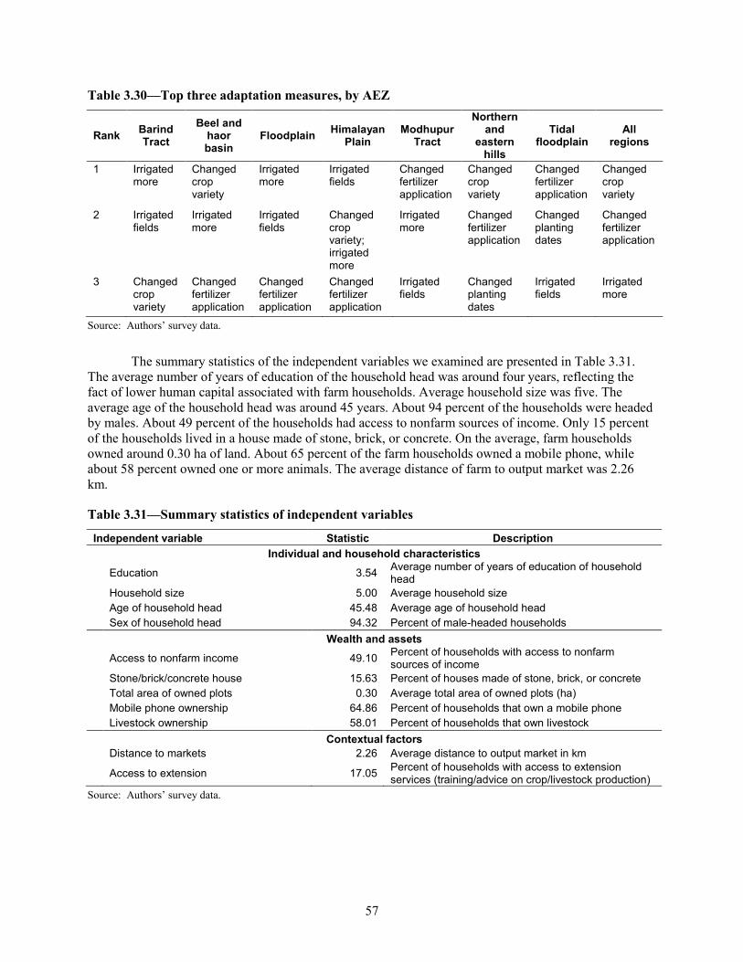
Table 3.30—Top three adaptation measures, by AEZ

Rank Barind Tract

Beel and haor basin

Floodplain Himalayan Plain

Modhupur Tract

Northern and

eastern hills

Tidal floodplain

All regions

1 Irrigated more

Changed crop variety

Irrigated more

Irrigated fields

Changed fertilizer application




2 Irrigated fields

Irrigated more

Irrigated fields

Changed crop variety; irrigated more

Irrigated more


Changed planting dates


3 Changed crop variety




Irrigated fields

Changed planting dates

Irrigated fields

Irrigated more


The summary statistics of the independent variables we examined are presented in Table 3.31. The average number of years of education of the household head was around four years, reflecting the fact of lower human capital associated with farm households. Average household size was five. The average age of the household head was around 45 years. About 94 percent of the households were headed by males. About 49 percent of the households had access to nonfarm sources of income. Only 15 percent of the households lived in a house made of stone, brick, or concrete. On the average, farm households owned around 0.30 ha of land. About 65 percent of the farm households owned a mobile phone, while about 58 percent owned one or more animals. The average distance of farm to output market was 2.26 km.

Table 3.31—Summary statistics of independent variables

Independent variable Statistic Description Individual and household characteristics

Education 3.54 Average number of years of education of household head

Household size 5.00 Average household size Age of household head 45.48 Average age of household head Sex of household head 94.32 Percent of male-headed households

Wealth and assets

Access to nonfarm income 49.10 Percent of households with access to nonfarm sources of income

Stone/brick/concrete house 15.63 Percent of houses made of stone, brick, or concrete Total area of owned plots 0.30 Average total area of owned plots (ha) Mobile phone ownership 64.86 Percent of households that own a mobile phone Livestock ownership 58.01 Percent of households that own livestock

Contextual factors Distance to markets 2.26 Average distance to output market in km

Access to extension 17.05 Percent of households with access to extension services (training/advice on crop/livestock production)


57

To capture access to extension services, farmers were asked whether they were able to obtain training and advice on crop and livestock production. Only a small percentage of those surveyed (17 percent) had access to extension. To control for differences in villages in such geographically dispersed AEZs, the study ran dummy village variables. Only the independent variables in Table 3.31 are presented in the probit results, since these are the ones of interest.

Table 3.32 presents the results of the probit adaptation model for the top three adaptation choices in the household survey: changing variety planted, irrigating more or intensifying irrigation of plots, and changing fertilizer application. Marginal effects (p-values) are reported for ease of interpretation. (The marginal effect is the expected change in the probability of adaptation given a unit change in an independent variable from the mean value, ceteris paribus.)

Table 3.32—Results of the probit adaptation model, marginal effects reported

Variable

Changed variety Irrigated more Changed fertilizer application

Coefficient P level Coefficient P level Coefficient P level

Sex of household head -0.083 0.433 0.045 0.673 0.073 0.407

Age of household head 0.002 0.188 0.003* 0.099 0.000 0.748

Household size 0.024* 0.067 0.025* 0.067 -0.002 0.822

Education 0.007 0.261 0.009 0.168 -0.003 0.583

Access to extension 0.087 0.166 0.051 0.462 -0.011 0.844

Distance to markets 0.016 0.164 -0.013 0.327 -0.003 0.738

Total area of owned plots -0.008 0.878 -0.069 0.252 -0.004 0.929 House made of concrete/brick/stone 0.036 0.600 0.079 0.307 0.067 0.271

Mobile phone ownership -0.001 0.981 0.048 0.392 0.164** 0.000

Livestock ownership 0.005 0.916 0.010 0.841 -0.017 0.679

Access to nonfarm income -0.011 0.821 0.012 0.813 -0.007 0.856

Pseudo R-square 0.3369 0.2968 0.0995

LR chi-square 308.48** 229.08** 102.24** Source: Authors’ survey data. Note: * Significant at 10 percent probability level. ** Significant at 1 percent probability level.

The survey found that only a few factors significantly influence these adaptive strategies (Table 3.32). Household size significantly influences whether farmers change the variety of the crop they are planting: Larger households are more likely to change variety as a response to perceived climate change, at 10 percent probability level. Increasing the household size by one member (from the mean of five household members) increases the probability of changing crop variety by 2.4 percent. These results suggest that having additional household labor, such as extended family members and older children, facilitates changing crop variety.

A similar result was found for a farmer’s decision to intensify irrigation in response to perceived climate change. Household size positively and significantly influences whether farmers irrigate more, at 10 percent probability level. Increasing the household size by one member increases the probability of intensifying irrigation by 2.5 percent. Moreover, age of the household head, which can represent experience, was found to positively and significantly influence the decision to irrigate more, at 10 percent probability level. A unit (1-year) increase in the age of the household head (from the mean age of 45 years old) results in a 3 percent increase in the probability of irrigating more in response to perceived climate change.

58

With regard to changing fertilizer application, results showed that having a mobile phone positively and significantly influences whether farmers change their fertilizer application in response to perceived climate change, at 1 percent probability level. Farmers with a mobile phone are 16 percent more likely to adopt this adaptation strategy. This may mean that ownership of a mobile phone facilitates better access to information on weather or climatic changes (such as drought or cyclones), which influences the decision on fertilizer application rates. Farmers can easily implement this type of adaptation measure once they obtain information on weather events.

It is noteworthy that for all three adaptation measures, access to extension does not affect the likelihood of their adoption. This may imply that what the extension officer says is not relevant or related to climate change adaptation or, alternatively, that farmers effectively spread the information to those who have not had an extension visit, making their implementation of these adaptation options equally likely.

59

4. CONCLUSIONS AND RECOMMENDATIONS

This report has presented the detailed results of modeling research on potential impacts of climate change on Bangladesh agriculture.

The results of our modeling of crop yields with climate change show that the projected impact of climate change varies greatly from crop to crop. Wheat, for example, may experience large negative shocks to yields, while maize may not be greatly impacted. Adaptation could reduce adverse impacts of climate change; in the noteworthy case of boro rice, there might even be yield gain effects from climate change.

For most crops, adaptation appeared to consist primarily of changing variety, but in the case of boro, adaptation was best done by changing the planting month. This result raises the issue of whether multicropping would allow the option of changing planting month; the answer is beyond the scope of this study, but future studies should examine the issue of crop rotations in relation to climate change. Other adaptation options explored were irrigation and the use of chemical or organic fertilizers. In some cases, irrigation could lead to yield improvements, and particularly when planting in the dry season, it makes cultivation possible. Fertilizers were shown to give significant productivity improvement, but climate change will slightly reduce the yield boost of fertilizers.

Our analysis introduces BanglaSPAM, prepared for this study together with the Bangladesh Policy Research and Strategy Support Program, which spatially interpolates harvest area, production, and yield for 17 crops or crop groups. It also presents three global landcover datasets, based on satellite data, which are used in our analysis for providing weights when aggregating statistics on crop yields. In addition, we provide findings relevant to Bangladesh from IFPRI’s IMPACT model.

Finally, key results from our household survey, which targeted agricultural practices and climate change responses, confirmed that Bangladesh farmers already perceive the impacts of climate change and have undertaken a variety of adaptation options. In particular, the survey indicated that of all climate change–related shocks, floods, waterlogging, and river erosion had caused the largest loss to rice production. Farmers in our survey had lost around 12 percent of their harvest, on average, to some kind of shock, with about half of that attributable to flooding-related issues. The second leading cause of rice crop loss was pest-related, responsible for the loss of around 3 percent of production. Taken together, the results indicated that adaption efforts in Bangladesh should include adjusting planting dates, using improved cultivars better suited for climate change, improving fertilizer applications, and exploring increased maize production, while bolstering flood and pest protection for farmers.

Recommendations We have developed a set of policy recommendations related to preparing agriculture in Bangladesh for the impact of climate change between now and 2050.

1. Use improved cultivars better suited for future climate through continued agricultural research, development, and extension.

This analysis indicates that when practiced together, using improved cultivars better suited for climate change and adjusting planting dates can lessen the impacts of climate change on yields, especially for rice, and in some cases actually results in better yields than before climate change. Importantly, irrigated boro rice can achieve higher yields under 2050 climate conditions when planted optimally with currently available optimal cultivars. According to the household survey results, the most common adaptive responses to climate change included changing crop variety (60 percent). Maintaining and improving farmers’ access to optimal cultivars will be critical in order to avoid yield losses as the climate changes over the next 40 years. Future research is expected to produce cultivars that will give even higher yields in climates of the future, pointing to the importance of continued research.

60

2. Adjust rice planting dates to new climatic realities. This analysis shows that an earlier planting date of boro rice is an attractive option to mitigate yield losses; however, it can interfere with aman rice harvest. These conflicts point to the need for further research into optimal crop rotations. Currently only 39 percent of farmers report changing planting dates as an adaptation strategy. Exploring the feasibility of adjusting planting dates and expanding farmers’ ability to do so will be important in the years to come.

3. Improve fertilizer efficiency. The analysis shows that losses in yield due to climate change can be compensated for, for many crops, by increasing the availability of nitrogen in the soil. This can be done using chemical fertilizers; however, they are costly inputs, and in conventional broadcast scattering many of the nutrients are lost either to the atmosphere or to below the root zone, where the crops cannot take advantage of them. The nutrients that go into the atmosphere contribute to the accumulation of greenhouse gases; some that travel below the root zone contribute to contaminated drinking water or to high concentrations in rivers and lakes. The government currently subsidizes fertilizers, and any improvement in efficiency will lead both to budgetary savings and savings to the farmer. One method may be to use urea briquettes (also known as USG, urea super granules), which are being promoted by the International Fertilizer Development Center; other cheap, efficient fertilizers, such as neem-coated urea pellets, may become viable in coming years. Improving soil fertility can also be done through such methods as use of animal manure, cover crops, crop rotations, and crop or agroforestry residue.

4. Explore expanded maize production. Our research identifies potential gains in maize yield when optimizing planting months and cultivars under a high-fertilizer-use scenario. In addition, the IMPACT model demonstrates that maize prices will increase by 209 percent by 2050—more than any other food commodity. While production of maize is relatively low compared with that of rice, expanding maize production or switching from rice to maize cultivation could produce future advantages.

5. Develop a plan for mitigating crop loss due to flooding-related issues. Of all climate change–related shocks, floods, waterlogging, and river erosion caused the largest loss to rice production. Farmers in our survey lost around 12 percent of their harvest, on average, to some kind of shock, with about half of that attributable to flooding-related issues. The beel and haor basin agroecological zone lost a full 30 percent of its harvest to flooding-related issues. Improving farmers’ ability to adapt to increasing rains and flooding will be important for this region, in particular.

6. Improve pest management. The second leading cause of rice crop loss was pest-related, responsible for loss of around 3 percent of production. Insects, rodents, and viruses caused the highest proportion of rice losses in Barind Tract (42 percent), Modhupur Tract (47 percent), and northern and eastern hills (58 percent). At the same time, pesticide use was highest among farm households in the Barind Tract, while the Modhupur Tract had the lowest mean pesticide use (1,116.60 taka/ha), followed by the Himalayan Plain (1,148.55 taka/ha) and the northern and eastern hills (1,284.28 taka/ha). Farmers in areas with low pesticide use may want to explore increasing application in order to offset rice losses, while those in the Barind Tract may need to explore improving pesticide efficiency, given that farmers there still experience significant losses despite high pesticide application rates.

61

REFERENCES

ADB (Asian Development Bank) and IFPRI (International Food Policy Research Institute). 2009. Building Climate Resilience in the Agriculture Sector in Asia and the Pacific. Mandaluyong City, Philippines: ADB. http://www.adb.org/publications/building-climate-resilience-agriculture-sector-asia-and-pacific.

Bangladesh, Bureau of Statistics. 2004. Labour Force Survey 2002-2003. Dhaka, Bangladesh: Ministry of Planning.

Bangladesh, Bureau of Statistics. 2008. Handbook of Agricultural Statistics in Bangladesh. Dhaka, Bangladesh: Ministry of Planning.

Bangladesh, Bureau of Statistics. 2010. Report of the Household Income and Expenditure Survey 2010. Dhaka, Bangladesh: Ministry of Planning.

Bangladesh, Ministry of Finance. 2011. Bangladesh Economic Review 2010. Dhaka, Bangladesh.

Bangladesh, MoEF (Ministry of Environment and Forest). 2005. Bangladesh National Adaptation Programme of Action (NAPA). Dhaka, Bangladesh.

Bangladesh Planning Commission, General Economics Division. 2005. Bangladesh: Poverty Reduction Strategy Paper. Washington: IMF.

Barkat, A., R. Faridi, S. N. Wadood, S. K. Sengupta, and S. N. M. Ehsanul Hoque. 2010. A Quantitative Analysis of Fertilizer Demand and Subsidy Policy in Bangladesh. Dhaka, Bangladesh: Manob Sakti Unnayan Kendro.

BCAS (Bangladesh Center for Advanced Studies). 2009. Policy Study on the Probable Impacts of Climate Change on Poverty and Economic Growth and the Options of Coping with Adverse Effect of Climate Change in Bangladesh. Dhaka, Bangladesh: General Economics Division, Planning Commission; United Nations Development Programme, Bangladesh.

Bryan, E., T. T. Deressa, G. A. Gbetibouo, and C. Ringler. 2009. “Adaptation to Climate Change in Ethiopia and South Africa: Options and Constraints.” Environmental Science and Policy 12 (4): 413–426.

Chowdhury, J. A., ed. 2005. Yearbook of Agricultural Statistics of Bangladesh. Dhaka, Bangladesh: Bureau of Statistics.

Hertel, T. W., and S. D. Rosch. 2010. “Climate Change, Agriculture, and Poverty.” Applied Economic Perspectives and Policy 32 (3): 355–385. http://aepp.oxfordjournals.org/content/early/2010/09/02/aepp.ppq016.full.

Hijmans, R. J., S. E. Cameron, J. L. Parra, P. G. Jones, and A. Jarvis. 2005. “Very High Resolution Interpolated Climate Surfaces for Global Land Areas.” International Journal of Climatology 25:1965–1978. www.worldclim.org.

IPCC (Intergovernmental Panel on Climate Change). 2000. Special Report: Emissions Scenarios, edited by N. Nakicenovic and R. Swart. Cambridge, UK: Cambridge University Press.

________. 2011. Model Output Described in the 2007 IPCC Fourth Assessment Report (SRES Scenarios), Multi-year Means. Updated May 16. Accessed June 7, 2011. http://www.ipcc-data.org/ar4/gcm_data.html.

Jones, P. G., P. K. Thornton, and J. Heinke. 2009. Generating Characteristic Daily Weather Data Using Downscaled Climate Model Data from the IPCC’s Fourth Assessment. Bonn, Germany; Nairobi, Kenya: Federal Ministry for Economic Cooperation and Development; International Livestock Research Institute. Accessed June 5, 2010. http://www.ccafs-climate.org/downloads/docs/Generating_Characteristic_Daily_Weather_Data_using_Downscaled_Climate_Model_Data_Jones_Thornton_Heinke_2009.pdf.

Masutomi, Y., K. Takahashi, H. Harasawa, and Y. Matsuoka. 2009. “Impact Assessment of Climate Change on Rice Production in Asia in Comprehensive Consideration of Process/Parameter Uncertainty in General Circulation Models.” Agriculture, Ecosystems and Environment 131 (3–4): 281–291.

Millennium Ecosystem Assessment. 2005. Ecosystems and Human Well-Being: Synthesis. Washington, DC: Island Press. http://www.unep.org/maweb/documents/document.356.aspx.pdf.

62

http://aepp.oxfordjournals.org/content/early/2010/09/02/aepp.ppq016.full

http://www.worldclim.org/

http://www.ipcc-data.org/ar4/gcm_data.html

Nelson, G. C., M. W. Rosegrant, J. Koo, R. Robertson, T. Sulser, T. Zhu, C. Ringler, et al. 2009. Climate Change: Impact on Agriculture and Costs of Adaptation. Washington, DC: International Food Policy Research Institute.

_______. 2010. The Costs of Agricultural Adaptation to Climate Change. Development and Climate Change Discussion Paper No. 4. Washington, DC: World Bank. http://siteresources.worldbank.org/EXTCC/Resources/407863-1229101582229/D&CCDP_4-Agriculture9-15-10.pdf.

Nelson, G. C., M. W. Rosegrant, A. Palazzo, I. Gray, C. Ingersoll, R. Robertson, S. Tokgoz, et al. 2010. Food Security, Farming, and Climate Change to 2050: Scenarios, Results, Policy Options. Washington, DC: International Food Policy Research Institute.

Parry, M. L., O. F. Canziani, J. P. Palutikof, P. J. van der Linden, and C. E. Hanson, eds. 2007. Climate Change 2007: Impacts, Adaptation and Vulnerability. Contribution of Working Group II to the Fourth Assessment Report of the Intergovernmental Panel on Climate Change. Cambridge, UK: Cambridge University Press.

Reid, H., and M. Alam. 2005. “Millennium Development Goals.” Tiempo: A Bulletin on Climate and Development 54:18–22.

Rosegrant, M. W., C. Ringler, S. Msangi, T. B. Sulser, T. Zhu, and S. A. Cline. 2008. International Model for Policy Analysis of Agricultural Commodities and Trade (IMPACT): Model Description. Washington, DC: International Food Policy Research Institute. www.ifpri.org/sites/default/files/publications/impactwater.pdf.

Sattar, S. A. 2000. “Bridging the Rice Yield Gap in Bangladesh.” In Bridging the Rice Yield Gap in the Asia–Pacific Region, edited by M. K. Papademetriou, F. J. Dent, and E. M. Herath, 58–68. Bangkok, Thailand: Food and Agriculture Organization Regional Office for Asia and the Pacific.

Tubiello, F. N., and C. Rosenzweig. 2008. “Developing Climate Change Impact Metrics for Agriculture.” The Integrated Assessment Journal 8 (1): 165–184.

UNDP (United Nations Development Programme). 2009. Policy Study on the Probable Impacts of Climate Change on Poverty and Economic Growth and the Options of Coping with Adverse Effect of Climate Change in Bangladesh. Dhaka, Bangladesh; New York: Planning Commission; UNDP.

UNPOP (United Nations Department of Economic and Social Affairs–Population Division). 2009. World Population Prospects: The 2008 Revision. New York. Downloaded from http://esa.un.org/unpd/wpp/.

White, J. W., G. Hoogenboom, B. A. Kimball, and G. W. Wall. 2011. “Methodologies for Simulating Impacts of Climate Change on Crop Production.” Field Crops Research 124 (3): 357–368.

World Bank. 2010a. World Development Report 2010: Development and Climate Change. Washington, D.C.

World Bank. 2010b. Economics of Adaptation to Climate Change: Synthesis Report. Washington: World Bank. Available at http://climatechange.worldbank.org/content/economics-adaptation-climate-change-study-homepage.

Yu, W., M. Alam, A. Hassan, A. S. Khan, A. Ruane, C. Rosenzweig, D. Major, et al. 2010. Climate Change Risks and Food Security in Bangladesh (Earthscan Climate). New York: Earthscan.

63

http://siteresources.worldbank.org/EXTCC/Resources/407863-1229101582229/D&CCDP_4-Agriculture9-15-10.pdf

http://siteresources.worldbank.org/EXTCC/Resources/407863-1229101582229/D&CCDP_4-Agriculture9-15-10.pdf

http://www.ifpri.org/sites/default/files/publications/impactwater.pdf

http://climatechange.worldbank.org/content/economics-adaptation-climate-change-study-homepage

http://climatechange.worldbank.org/content/economics-adaptation-climate-change-study-homepage

RECENT IFPRI DISCUSSION PAPERS

For earlier discussion papers, please go to www.ifpri.org/pubs/pubs.htm#dp. All discussion papers can be downloaded free of charge.

1280. Demand for weather hedges in India: An empirical exploration of theoretical predictions. Ruth Vargas Hill, Miguel Robles, and Francisco Ceballos, 2013.

1279. Organizational and institutional issues in climate change adaptation and risk management:Iinsights from practitioners’ survey in Bangladesh, Ethiopia, Kenya, and Mali. Catherine Ragasa, Yan Sun, Elizabeth Bryan, Caroline Abate, Atlaw Alemu, and Mahamadou Namori Keita, 2013.

1278. The impact of alternative input subsidy exit strategies on Malawi’s maize commodity market. Mariam A. T. J. Mapila, 2013.

1277. An ex ante analysis of the impact and cost-effectiveness of biofortified high-provitamin A and high-iron banana in Uganda. John L. Fiedler, Enoch Kikulwe, and Ekin Birol, 2013.

1276. Local warming and violent conflict in north and south Sudan. Margherita Calderone, Jean-Francois Maystadt, and Liangzhi You, 2013.

1275. Comprehensive food security and vulnerability analysis: Nigeria. Oluyemisi Kuku-Shittu, Astrid Mathiassen, Amit Wadhwa, Lucy Myles, and Akeem Ajibola, 2013.

1274. Targeting technology to reduce poverty and conserve resources: Experimental delivery of laser land leveling to farmers in Uttar Pradesh, India. Travis J. Lybbert, Nicholas Magnan, David J. Spielman, Anil Bhargava, and Kajal Gulati, 2013.

1273. The logic of adaptive sequential experimentation in policy design. Haipeng Xing and Xiaobo Zhang, 2013.

1272. Dynamics of transformation: insights from an exploratory review of rice farming in the Kpong Irrigation Project. Hiroyuki Takeshima, Kipo Jimah, Shashidhara Kolavalli, Xinshen Diao, and Rebecca Lee Funk, 2013.

1271. Population density, migration, and the returns to human capital and land: insights from Indonesia. Yanyan Liu and Futoshi Yamauchi, 2013.

1270. Reverse-share-tenancy and marshallian inefficiency: Landowners’ bargaining power and sharecroppers’ productivity. Hosaena Ghebru Hagos and Stein T. Holden, 2013.

1269. The child health implications of privatizing Africa’s urban water supply. Katrina Kosec, 2013.

1268. Group lending with heterogeneous types. Li Gan, Manuel A. Hernandez, and Yanyan Liu, 2013.

1267. Typology of farm households and irrigation systems: Some evidence from Nigeria. Hiroyuki Takeshima and Hyacinth Edeh, 2013.

1266. Understanding the role of research in the evolution of fertilizer policies in Malawi. Michael Johnson and Regina Birner, 2013.

1265. The policy landscape of agricultural water management in Pakistan. Noora-Lisa Aberman, Benjamin Wielgosz, Fatima Zaidi, Claudia Ringler, Agha Ali Akram, Andrew Bell, and Maikel Issermann, 2013.

1264. Who talks to whom in African agricultural research information networks?: The Malawi case. Klaus Droppelmann, Mariam A. T. J. Mapila, John Mazunda, Paul Thangata, and Jason Yauney, 2013.

1263. Measuring food policy research capacity: Indicators and typologies. Suresh Chandra Babu and Paul Dorosh, 2013.

1262. Does freer trade really lead to productivity growth?: Evidence from Africa. Lauren Bresnahan, Ian Coxhead, Jeremy Foltz, and Tewodaj Mogues, 2013.

1261. Data needs for gender analysis in agriculture. Cheryl Doss, 2013.

1260. Spillover effects of targeted subsidies: An assessment of fertilizer and improved seed use in Nigeria. Lenis Saweda Liverpool-Tasie and Sheu Salau, 2013

1259. The impact of irrigation on nutrition, health, and gender: A review paper with insights for Africa south of the Sahara. Laia Domenech and Claudia Ringler, 2013.

1258. Assessing the effectiveness of multistakeholder platforms: Agricultural and rural management councils in the Democratic Republic of the Congo. Thaddée Badibanga, Catherine Ragasa, and John Ulimwengu, 2013.

INTERNATIONAL FOOD POLICY RESEARCH INSTITUTE

www.ifpri.org

IFPRI HEADQUARTERS 2033 K Street, NW Washington, DC 20006-1002 USA Tel.: +1-202-862-5600 Fax: +1-202-467-4439 Email: [email protected]

mailto:[email protected]

agriculture and adaptation in bangladesh -...

Documents