aggregation problems in the measurement of capital aggregation problems in the measurement of...
TRANSCRIPT
This PDF is a selection from an out-of-print volume from the National Bureauof Economic Research
Volume Title: The Measurement of Capital
Volume Author/Editor: Dan Usher, editor
Volume Publisher: University of Chicago Press
Volume ISBN: 0-226-84300-9
Volume URL: http://www.nber.org/books/ushe80-1
Publication Date: 1980
Chapter Title: Aggregation Problems in the Measurement of Capital
Chapter Author: W. Erwin Diewert
Chapter URL: http://www.nber.org/chapters/c7171
Chapter pages in book: (p. 433 - 538)

8 Aggregation Problems in the Measurement of Capital W. E. Diewert
8.1 Introduction and Overview
In his Introduction to this volume, Dan Usher has provided us with a rather comprehensive discussion on the purposes of capital measure- ment as well as the problems of defining capital in the context of a specific purpose.
With Usher’s introduction in mind, the scope of the present paper can readily be defined: I will concentrate on the problems of defining and measuring capital in the context of estimating production functions and measuring total factor productivity, with particular emphasis on the associated index number problems.
However, before discussing the special problems involved in aggre- gating capital, I will first discuss the general problem of aggregating over goods in section 8.2 and the general problem of aggregating over sectors in section 8.3. The material presented in these sections is for the most part not new, although much of it is fairly recent and not widely known. Usher’s new definition of real capital is discussed in section 8.2.6 along with some other definitions.
I n section 8.4 I discuss some of the aggregation problems that are specifically associated with capital. In particular, the problem of de- fining capital as an instantaneous stock or a service flow is discussed along with the concomitant problems of measuring depreciation.
In section 8.5 I present some new material on the measurement of total factor productivity and technical progress. In this section, capital
W. E. Diewert is associated with the Department of Economics at the Uni-
The author is indebted to E. R. Berndt, C. Blackorby, P. Chinloy, M. Denny,
versity of British Columbia, Vancouver.
L. J. Lau, D. Usher, and F. Wykoff for helpful comments.
433

434 W. E. Diewert
does not play a more important role than any other factor of produc- tion, so that one could question its inclusion in a paper that is supposed to be restricted to capital aggregation problems. However, past discus- sions of technical change have emphasized the possibility that technical change may be embodied in new capital goods (see Jorgenson 1966)’ and thus I decided to include section 8.5.
One of the most difficult problems in the measurement of capital is the problem of new goods. This is of course not specific to capital, and so in section 8.6 I present some suggestions for solving the new goods problem in general.
In section 8.7 I briefly consider a problem that occurs when measur- ing capital as well as other inputs and outputs: the problem of aggregat- ing over time; that is, How should “monthly” estimates of a capital good be constructed? or, given monthly estimates, How should we construct an annual estimate of the capital component?
In section 8.8 I conclude by making some concrete recommendations to national income accountants based on the material in the previous sections. Some mathematical proofs are contained in the Appendix.
8.2 Methods for Justifying Aggregation over Goods
8.2.1 Price Proportionality: Hicks’s Aggregation Theorem
Hicks (1946, pp. 312-13) showed (in the context of twice-differ- entiable utility functions) that if the prices of a group of goods change in the same proportion, that group of goods behaves just as if it were a single commodity. This aggregation theorem and the homogeneous weak separability method (which will be discussed in the following section) are the two most general methods we have for justifying ag- gregation over goods. Alternative statements and proofs of Hicks’s aggregation theorem in the consumer context can be found in Wold (1953, pp. 109-lo), Gorman (1953, pp. 76-77), and Diewert (19784.
Versions of Hicks’s aggregation theorem also exist in the producer context, particularly in the context of measuring real value added (see Khang 1971 ; Bruno 1978; Diewert 1978~) . Below, I sketch yet another version of Hicks’s aggregation theorem in the producer context, a ver- sion that does not make use of any restrictive differentiability assump- tions.
Suppose there are N + M goods that a given firm can produce or use as an input and that the set of feasible input-output combinations of goods is a set S = { (x,y) } = { (x1,x2, . . . ,xy,y1,y2, . . . , y N ) } , where x,, represents the quantity of good n produced (used as an input if x, < 0) and ym represents the quantity of good N + rn produced by

435 Aggregation Problems in the Measurement of Capital
the firm (used as an input if ym < 0). We assume that the firm can buy or sell the first N goods at the positive prices ( w l , w p , . . . ,wN) = w ) ) ON1 and the last M goods at the positive prices ( p 1 , p 2 , . . . , p ~ ) = p ) ) 0,. We assume that the firm behaves competitively and attempts to solve the following microeconomic profit-maximization problem:
( 1 1 max,,v{w*x + p-y : ( x , y ) E S } 3 II (w,p) .
The solution to the above profit-maximization problem (if one ex- ists)2 is a function of the prices w,p that the producer is facing and is called the (micro) profit function TI. It can be shown (see McFadden 1978 or Diewert 1 9 7 3 ~ ) that under suitable regularity conditions on the technology S, the profit function completely characterizes the underly- ing technology. This duality property will prove very useful in subse- quent sections of this chapter.
The firm's gross3 or restricted4 or variable5 profit function IT* is de- fined as
(2)
The usual interpretation of the maximization problem (2) is that the firm is maximizing only with respect to its variable inputs and output x, while the inputs (and or outputs) y remain fixed in the short run. It can also be shown under suitable regularity conditions on S that a knowledge of the variable profit function II* is sufficient to completely determine the underlying technology S.6 Thus, we will use the variable profit function to define an aggregate technology.
Suppose the prices of the first N goods vary in strict proportion; that is,
( 3 )
where p o > 0 is a scalar that varies over time while the proportionality constants (alp2, . . . ,aN) - a ) ) ON remain fixed over time.
We can now define a macro technology set S, using the variable profit function II* and the vector of constants a as follows:
(4) S, = { ( Y o J ) : Y O 5 IT* ( a , y ) , where y is such that there exists an x such that ( x , y ) d } .
II*(w,y) E maxo{w*x : ( x , y ) d } .
(w1,wz,. . . ,WN) = (Po% p o a 2 , * * * , P o a N ) ,
We will see that yo can be interpreted as an aggregate of the compo- nents of x ; that is, y o = w*x/po . It is easy to show that the macro tech- nology set S, inherits many of the properties of the micro technology set S. For example, if S is a convex set7 (which is a generalization of the Hicksian [ 1946, p. 811 diminishing marginal rates of transformation reg- ularity conditions on s), then S, is also a convex set.* Moreover, if S exhibits constant returns to scale,g then S, also exhibits constant returns to scale.1°

436 W. E. Diewert
Given that the macro technology set S, has been defined, we may now define the macro profit maximizations problem
( 5 ) max, ,!/{POYO + P'Y : ( Y o , Y ) 4 = W P 0 , P ) . 0
The following theorem shows that if the price proportionality assump- tion in ( 3 ) is satisfied, then the macro profit maximization problem (5) is completely consistent with the underlying "true" micro profit maxi- mization problem ( 1 ).
( 6 ) Thorem: If ( x * , y * ) is a solution to the micro profit maximization problem ( 1 ) and the price proportionality assumption ( 3 ) holds, then (y*",y*) is a solution to the macro profit maximization ( 5 ) , where the aggregate y*o is defined by
(7) y*o = w*x*/po .
Note that, if the vector of constants a is known, the aggregate y*o can be calculated from observable price and quantity data.
The theorem above shows that, if the factors of proportionality ( ~ I , ( Y z , . . . , a ~ ) = a remain constant over time, then the true micro technology S can be replaced by the macro technology S,. However, in most practical situations, a will not remain constant over time, though it may be approximately constant, in which case the set S, will be ap- proximately constant also, and this approximate constancy may suffice for empirical work. Perhaps a concrete example would make this point clearer.
Suppose the technology of the firm can be represented by a translog variable profit function1' II* which is defined by the following equation:
N N N
sj In yri + '/z S 2 ail, In y; In yrk, I - 1 k = l
where w' = (wrl,wrz, . . . ,wrN) ) ) 0, is the vector of prices for the first N goods in period r where r = 1,2, . . . ,T ( x r = (xr l , x r2 , . . . ,x'N) is the corresponding quantity vector) and y" = (yrl ,yr2, . . . ,y;) ) ) OM is a vector of purchases and sales of the last M goods in period r ( p r = (pr1,pr2, . . . , p r l ) is the corresponding vector of prices). Because the logarithm of a negative number is not defined, we have temporarily changed our sign convention and made all components of y' positive whether the corresponding goods are outputs or inputs. Thus if the N + Mth good during period r is an output, yTm > 0 and prnL > 0; how-

437 Aggregation Problems in the Measurement of Capital
ever, if the N + m th good during period r is an input, set yrm > 0 equal to the absolute value of the amount of input and set pr, < 0 equal to minus the input price.
The technological parameters Pih in (8) satisfy the symmetry re- strictions Pih = Phi for 1 < i < h < N , and the satisfy the restric- tions aJh = St j for 1 5 j < k 2 M . In order that the translog variable profit function II* ( w , y ) be linearly homogeneous in w, the following restrictions on the parameters in (8) must be satisfied:
(9) N N N
i=l h=l i=l 2 P i = l ; 2 P i h = O f o r i = 1 , 2 , ..., N ; 2
yij = 0 for j = 1,2, . . . ,M. Now let the wr prices vary approximately proportionately over time;
that is,
( 1 0 ) w' = (w+1,w'*, . . . ,wrN)
= (prOaleEr'I ,pr0(Y2eE+2, . . . , p ' O a N e C r N ) ,
where pro represents the general level of prices of the first N goods, the ai represent fixed factors of proportionality, and the eri represent per- turbations in these fixed factors of proportionality.
If we deflate II* (w',yr) = wr*xr by pOr (which converts a nominal value added into a "real" value added), then (10) and (8) yield
M Y
where the Hicks's aggregate approximation error E' in period r is defined as
A' s
i=l h = l + 95 2 8 PihEriErh.
Note that the left-hand side of ( 1 1 ) is observable (if pro is known), while the right-hand side is a conventional translog production function in the quantities y' if the error term e7. is neglected. Note how shifts in the price proportionality constants (Y 3 (a1,,a2, . . . ,aN) will systemati- cally shift this translog production function.
438 W. E. Diewert
If the perturbations E‘, defined above are such that EE‘,=O and EE‘& = S,W,~ for i,h = 1,2, . . . ,N and r,s = 1,2, . . . ,T, where E denotes the expectation operator and Srt equals 0 if r # t but SYt = 1 if r = t , then it is trivial to show that the error E‘ will have a constant b i a P that will be absorbed into the constant if regression techniques are used in order to estimate the parameters of ( 11 ) . Thus, with the above stochastic assumptions,13 the production function that corresponds to the macro technology set S, could be unbiasedly estimated up to a scaling factor, provided that the underlying technology S could be ade- quately approximated by the translog variable profit function II* defined by ( 8 ) . This last proviso will be satisfied for moderate variations in prices and quantities, since the translog variable profit function can pro- vide a second-order approximation to an arbitrary twice-differentiable variable profit function that in turn provides a complete description of the underlying technology S under suitable regularity conditions.
Thus it appears that the assumption of approximate price propor- tionality provides a rather powerful justification for aggregating over commodities.
Note that the aggregation method studied in this section did not re- strict the technology in any essential way; rather, the set of prices that producers faced was restricted. I n the following section, a method of aggregating over commodities is outlined that depends on the technol- ogy’s satisfying certain restrictive assumptions.
8.2.2 Homogeneous Weak Separability
The second major method justifying commodity aggregation is due to Leontief (1947) and Shephard (1953, pp. 61-71; 1970, pp. 145-46; see also Solow 1955-56; Green 1964; Arrow 1974; Geary and Morish- ima 1973), and I will outline this method below. To cover both pro- ducer and consumer theory applications of this method of aggregation, we assume cost minimizing (instead of profit maximizing) behavior on the part of producers.
Suppose the microeconomic production (or utility) function f * where u = f * (x ,z) is output (or utility), x >_ 0, is a nonnegative N-dimen- sional vector of commodity inputs to be aggregated, and z 2 OM is an M-dimensional vector of “other” commodity inputs. The producer’s (or consumer’s) total minimum cost function is defined as:
(13)
where p = ( p , , p I , . . . ,p\) ) ) O\. is a vector of positive input prices and w = (w1,w2, . . . ,w,[) ) ) O,, is a vector of “other” input prices. The Shephard (1953, 1970) duality theorem (see also Samuelson 1953-54; Uzawa 1964; McFadden 1978; Hanoch 1978; and Diewert 1971) states
C* ( u ; p,w) = min, {pax + w-z: f * ( x , z ) >_ u},

439 Aggregation Problems in the Measurement of Capital
that, under certain regularity conditions, the total cost function C* com- pletely determines the production function f*. Thus restrictions on the production function f* translate into restrictions on the cost function C* and vice versa. We will make use of this fact below.
To justify the aggregation of the commodities x, Shephard assumed that x was homogeneously weakly sepurable14 from the “other” com- modities z ; that is, he assumed that the micro function f* could be writ- ten as
(14) f* (x,z) = frf(x) ,zl,
where is a macro production (or utility) function (satisfying the same regularity conditions as f* ) and f is an aggregator function that is as- sumed to satisfy the following regularity conditions.
(15) Conditions on f : i) ii)
iii)
f is defined for x ) ) ON and f(x) > 0 (positivity); f(U) = Af(x) for A > 0, x ) ) ON (linear homo- geneity) ;
0 5 A 5 1, x1 ) ) O N , x2 ) ) OAT( concavity). f(U1 + (1 - A)X’) 2 Af(xl) + ( 1 - A)f(X2) for
The macro function i has a cost function dual defined by
(16) e ( u ; po,w) = min,,,{po + w: J(Y,z) 2 u>,
where P o > 0 is the price of the aggregate, y. The aggregator function f also has a total cost function dual defined by
(17) C(Y; P I = minl{p*x: f(x) 2 Y}
= y min,/,{p*x/y:f(x/y) 2 l} using (15.ii)
= Y C ( P ) .
It turns out that the unit cost function c ( p ) satisfies the same regularity conditions as f ; that is, c(p) is positive, linearly homogeneous, and concave for p ) ) ON (see Samuelson 1953-54; Diewert 19743). Moreover, given a unit-cost function c ( p ) satisfying the conditions (15), the production function dual may be defined as15
(18) f(x) = l/mux,{c(p): p*x = 1, p 2 ON}. With the above preliminaries disposed of, we can now outline the
Shephard-Solow-Arrow results. Suppose p**x* + w**z* = C* (u*; p*,w*); that is, x*,z* is a solution to the micro cost minimization prob- lem (13) when micro prices p*,w* (and utility or output u*) prevail. If the micro function f* is homogenously weakly separable (i.e., f * satisfies eq. 14) and if the functional form for the aggregator function f

440 W. E. Diewert
is known (or the functional form for its unit-cost function c ( p ) is known), then the aggregate y* can be defined as
(19) y* = f ( x * ) (or y* = p * * x * / c ( p * ) ) ,
and the price of the aggregate may be defined as
(20) p * o =p**x*/f(x*) (or p * o = c ( p * ) ) ,
and ~ * ~ y * + w**z* = f ( u * ; p * , , w * ) ; that is, y*,z* is a solution to the macro cost minimization problem (16) with prices ~ * ~ , w * (and utility or output u * ) .I6
There are, of course, at least two problems with this aggregation method: ( a ) the micro function f* may not be homogeneously weakly separable in practice, and ( b ) the functional form for the aggregator function f is generally unknown. In the remainder of this section, our attention will be directed toward solving the second difficulty.
Let p‘ ) ) O N , w‘) ! OM for r = 0,1, . . . ,T. If xr,zr is a solution to min,.,{pr*x + W*Z: ?[f(x) ,z] 2 u‘} and if 3 is increasing in its first argument, it is easy to see that xr must be a solution to the following aggregator maximization problem.
(21 1 In other words, if an economic agent wishes to minimize the cost of
achieving a certain utility or output !eve1 when the micro function f * is weakly separable (i.e., f*(x,z) = f[f(x),z]) and the macro function 3 is increasing in its first argument, then the “intermediate input” (or “real value added” or “category subutility”) f(x) must be a maximum subject to an expenditure constraint.
Notice that (21 ) involves only the (unknown) aggregator function f and observable prices and quantities, {pr,xr} for r = 0,1, . . . ,T. If f is differentiable, then the first-order necessary conditions for a maximum yield the following identity after the Lagrange multiplier is eliminated :
( 2 2 ) Lemma: (Konyus and Byushgens 1926, p. 155; Hotel- ling 1935, pp. 71-74; Wold 1944, pp. 69-71). Suppose f is differentiable and x‘ > ON is a solution to max,{f(x) : pr*x i pr*xr, x 2 O x } , where pr ) ) O N . Then
max,{f(x) : p‘*x I pr-xr; x 2: ON} r = 0,1, . . . ,T.
where v f(xr) is the vector of first-order partial deriva- tives evaluated at xr.
Corollary:1i If f is also homogeneous of degree one (i.e., f ( h x ) = h f ( x ) for every h > 0), then

441 Aggregation Problems in the Measurement of Capital
The above corollary suggests the following Method Z (due to Arrow 1974) for determining the aggregator function f given the micro data {p+,x'}, r = 0,1,2, . . . ,T: simply assume a convenient functional form for f and use the relations (23) to econometrically estimate the un- known parameters. For example, suppose that f is the homogeneous translog function (Christensen, Jorgenson, and Lau 1971 ) :
(24) N A"
n=1 j=1 k = l lnf(xr> = P o + 8 P J n x ' n + '/z 2 2
pjkln xrj In x k , r = 0,1, . , . ,T, N N
n = l k = l where 8 Pa = 1, p j k = p k j and 2
p j k = 0 for j = 1,2, . . . ,N. With the above parameter restrictions, f turns out to be linearly
homogeneous. Application of (23) yields the following system of equa- tions that is linear in the unknown parameters:
where p* E (prl,pr2, . . . , p r N ) and xr = (xr1,x'2, . . .,xr~). Notice that the parameter Po is not identified, but once the other parameters are determined, an estimate for Po may be obtained by solving f ( x o ) = 1 for Po (base period normaZization) . For an econometric application of this method in the context of estimating a real value-added production function, see Berndt and Christensen (1973).
Instead of econometrically estimating the parameters of the aggregator function f , we may attempt to estimate the parameters of its unit cost function, c ( p ) . In this context, the following result is useful.
(26) Lemma: (Shephard 1953, p. 11; Samuelson 1953-54) If f satisfies (IS), pr*xr = minz{pr*x: f ( x ) 2 f ( x r ) } = c(pr)f(xr) for r = 0,1, . . .T, and the unit cost function c is differentiable at p', then
x r = k c ( p r ) f ( x r ) , r = 0 , 1 , . . . ,T
(27) CorolZary:18 xr/pr*xr = ' v l c (pr ) / c (pr ) , Y = 0,1,. . . ,T.
The above corollary suggests the following Method ZZ (also due to Arrow 1974) for determining the dual c to the aggregator function f

442 W. E. Diewert
given the micro data {pc,xr}, r = 1,2, . . . ,T: assume a functional form for c ( p ) and use the relations (27) to estimate the unknown parameters of c ( p ) . For example, suppose that c is the translog unit cost function (Christensen, Jorgenson, and Lau 197 1 ) :
(28) N A"
n = l j=1 k = l In c(P') =yo+ 2 y h p r , + 1/2 8 8
yfk r 0 for j = 1,2, . . . ,N. Application of Shephard's lemma (27) yields the following system of
equations that is linear in the unknown parameters: N
Notice that the parameter yo is not identified, but once the other parameters are determined an estimate for yo may be obtained by soh- ing the equation pO*xO/c(po) = 1 (base period normalization), which makes f ( x o ) = 1 .
Note that the translog unit cost function generates an aggregator func- tion via (1 8 ) that does not in generall9 coincide with the translog ag- gregator function defined by (24). Thus, in general, the two translog functional forms correspond to different tastes or technologies, although either functional form can approximate the same underlying (differen- tiable) technology to the second order.
At this point J should mention Method ZZZ for determining the ratio of the aggregates, f(xr)/f(xO). This final method involves assuming a functional form for the aggregator function f that is consistent with an index number formula (which is a function of observable prices and quantities for the two periods under consideration). The method as- sumes that X" is a solution to the aggregator maximization problem de- fined by (21>,2" and it will be studied in greater detail in section 8.2.4. When reading section 8.2.4, recall that it was the assumption of ex- penditure minimizing behavior (which is consistent with profit maximiz- ing behavior), plus the assumption that the technology was homo- geneously weakly separable in the x goods that led us to conclude that x" was a solution to the aggregator maximization problem max,{f(x) : PX 2 P+*x'}, where f is the linearly homogeneous aggregator function.
In the next section, I outline another method for aggregating over goods, a method due to FranCois Divisia (1926).
443 Aggregation Problems in the Measurement of Capital
8.2.3 The Divisia Index and Various Discrete Approximations
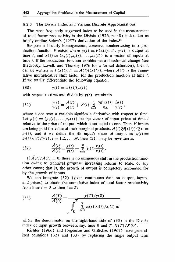
The most frequently suggested index to be used in the measurement of total factor productivity is the Divisia (1926, p. 40) index. Let us briefly outline Solow’s (1957) derivation of the index.21
Suppose a linearly homogeneous, concave, nondecreasing in x pro- duction function F exists where y ( t ) = F ( x ( t ) ; t ) , y ( t ) is output at time t, and x ( t ) = (xl(t),x2(t), . . . ,xAr(t)) is a vector of inputs at time t. If the production function exhibits neutral technical change (see Blackorby, Lovell, and Thursby 1976 for a formal definition), then it can be written as F ( x ( t ) ; t ) = A ( t ) f ( x ( t ) ) , where A ( t ) is the cumu- lative multiplicative shift factor for the production function at time t . If we totally differentiate the following equation
(30)
with respect to time and divide by y ( t ) , we obtain
Y (t) = A (t)f(x(t) 1
where a dot over a variable signifies a derivative with respect to time. Let p ( t ) I ( p l ( t ) , . . . , p N ( t ) ) be the vector of input prices at time t relative to the price of output, which is set equal to one. Then, if inputs are being paid the value of their marginal products, A ( t ) a f [ x ( t ) ] / a x 4 = pi(t), and if we define the ith input’s share of output as q ( t ) = p 6 ( t ) x i ( t ) / y ( t ) , i E 1 , 2 , . . . ,N, then (31) may be rewritten as
If A. ( t ) /A ( t ) = 0, there is no exogenous shift in the production func- tion owing to technical progress, increasing returns to scale, or any other cause; that is, the growth of output is completely accounted for by the growth of inputs.
We can integrate (32) (given continuous data on output, inputs, and prices) to obtain the cumulative index of total factor productivity from time t = 0 to time t = T :
A ( T ) - Y ( T ) / Y ( O ) A(O) -- (33) s,’ {Zl s ( t ) &(t) /xdt) dt ’
e
where the denominator on the right-hand side of (33) is the Divisia index of input growth between, say, time 0 and T , X ( T ) / X ( O ) .
Richter (1 966) and Jorgenson and Griliches (1967) have general- ized equations (32) and (33) by replacing the single output term

444 W. E. Diewert
Y ( t ) / y ( t ) in (32) with a share-weighted average of the growth rates of many outputs, and the term y ( T ) / y ( O ) in (33) with a Divisia index of output growth.
Since the right-hand sides of (32) and (33) are in principle ob- servable, the technical change term A ( t ) can, in principle, be esti- mated.22 But in practice data do not come in nice continuous series; rather they come at discrete intervals. Thus the continuous formulas (32) and (33) must be approximated using discrete data.
Let us now introduce some new notation that is appropriate when data come at discrete intervals. Let the vector of period r inputs be x' = (xrl,xrZ, . . . ,xTN) and period r prices be p' = (p'l,p'z, . . . , p k ) for r = 0,l.
Denote the denominator of (33) as X ( l ) / X ( O ) , when T = 1. If the input shares are approximately constant, then In X( 1 ) / X ( 0) ap-
proximately equals 8 siln xIi/xoi. For any number z close to 1 , In
z can be accuratel;=ipproximated by -1 + z , so that X ( l ) / X ( O )
approximately equals 2 sixli /xoi. Thus the Divisia index of input growth
X(l)!X(O) can be approximated by a share-weighted rate of growth of the quantity relatives x l i /x0 , , i = 1,2, , . . , N . If we choose base- period shares, the resulting index is the Laspeyres quantity index Qr,:
N
N
i= l
(34) N
1 =? where p0*xr 5 8 poixri denotes the inner product between the vectors
p o and x', r = 0,l. On the other hand, if we choose current-period prices and base-period quantities to form shares, the resulting index is the Paasche quantity index Qp:
(35)
A third way of approximating the share-weighted rate of growth of inputs that apepars in (32) would be to take a geometric mean of the index QL and Q p :
(36) Q 2 (po ,p l ; x ' , x~) = (po*~1p1*~1/po*~Op1*~o)1/2.
The index Q2 is Irving Fisher's (1922) ideal quantity index. The price index that corresponds to QZ is P2 defined implicitly by Fisher's weak factor reversal test:
(37) P2 (p' , ,~'; x',x') Q ~ ( ~ I O , ~ ~ , X ~ , X ~ ) = p * * x l / p 0 * x o ;
that is, the product of the price index times the quantity index equals the expenditure ratio between the two periods. Fisher called P2 and QZ
445 Aggregation Problems in the Measurement of Capital
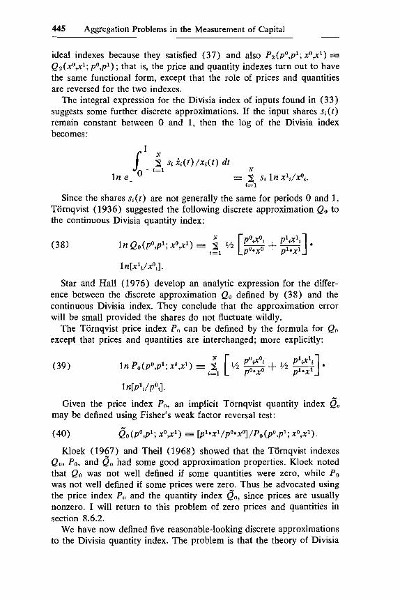
ideal indexes because they satisfied (37) and also P2(po ,p1; xo ,x l ) = Q 2 (xo,xl; p o , p l ) ; that is, the price and quantity indexes turn out to have the same functional form, except that the role of prices and quantities are reversed for the two indexes.
The integral expression for the Divisia index of inputs found in (33) suggests some further discrete approximations. If the input shares si( t ) remain constant between 0 and 1, then the log of the Divisia index becomes:
Since the shares s i ( t ) are not generally the same for periods 0 and 1, Tornqvist ( 1936) suggested the following discrete approximation Qo to the continuous Divisia quantity index:
(38)
1 n[xldxOi].
Star and Hall (1976) develop an analytic expression for the differ- ence between the discrete approximation Qo defined by ( 3 8 ) and the continuous Divisia index. They conclude that the approximation error will be small provided the shares do not fluctuate wildly.
The Tornqvist price index Po can be defined by the formula for Qo except that prices and quantities are interchanged; more explicitly:
(39)
1 n[P1i/pOil.
Given the price index Po, an implicit Tornqvist quantity index may be defined using Fisher's weak factor reversal test:
.-, (40) Qo (po ,p l ; X',X') E [ p ' * ~ ' / p ~ * ~ ~ ] / P o (po,p'; x',x').
Kloek (1967) and Theil (1968) showed that the Tornqvist indexes Qo, Po, and Qo had some good approximation properties. Kloek noted that Qo was not well defined if some quantities were zero, while P o was not well defined if some prices were zero. Thus he advocated using the price index P,, and the quantity index Qo, since prices are usually nonzero. I will return to this problem of zero prices and quantities in section 8.6.2.
We have now defined five reasonable-looking discrete approximations to the Divisia quantity index. The problem is that the theory of Divisia
446 W. E. Diewert
indexes outlined above does not tell us which discrete index number formula should be used in empirical applications, even though it is known that the Laspeyres and Paasche quantity indexes can differ con- siderably from the other indexes.23
It turns out that the economic theory of exact index numbers24 en- ables us to discriminate more sharply among the above index number formulas. I will briefly outline this theory.
8.2.4 Exact and Superlative Index Number Formulas
Suppose the production function (or aggregator function) is y = f(xl ,x2, . . . ,xN) = f ( x ) , where y is output (or the aggregate), x is a vector of inputs (or goods to be aggregated), and f is a nondecreasing, linearly homogeneous and concave function. Suppose further that, given a positive vector of input prices p = (p1,p2, . . . , p N ) , the producer at- tempts to minimize the cost of producing a given output level. The solution to the cost minimization problem is the total cost function C ( y ; p ) , which decomposes into a unit-cost function c ( p ) times the out- put level owing to the linear homogeneity of the aggregator functior f;25 that is,
(41 1 C ( y ; p ) = minr{p*x: f (x) = y } = c ( p ) y .
It is natural to identify c ( p ) with the price of output; that is, as being the price of the aggregate good y .
Suppose we are given price and quantity data for two periods, po,pl ,xo,xl . Define a price index simply as a function P of prices and quantities, P(pO,pl ;xo ,x l ) , while a quantity index Q(po,p l ;xo ,x l ) is an- other function of prices and quantities for the two periods. We gen- erally assume that the price and quantity indexes satisfy Fisher's weak factor reversal test; that is, P and Q satisfy
A given functional form for a quantity index Q is defined to be exact for a functional form for the aggregator function f if given output levels yo ,y l , input price vectors po,p1;x0 a solution to the period 0 cost mini- mization problem (41) and x1 a solution to the period 1 cost minimiza- tion problem (4 1 ) , then
(43)
for all y o > 0, y 1 > 0, p o ) ) O N , p1 ) ) Similarly, a given functional form for a price index P is defined to be exact for a functional form for the aggregator function f (and its derived unit cost function c ) if given output levels yo ,y l , input price vectors po,pl;xr a solution to the period r cost minimization problem (41) for r = 0.1, then

447 Aggregation Problems in the Measurement of Capital
(44) C(P1)/C(PO) = P(pO,pl; xO,xl).
Thus the quantity index Q equals the ratio of the “outputs” yl/yo, and the price index P equals the ratio of the unit costs (or the ratio of the “prices” of the “outputs”) c ( p l ) / c ( p o ) , provided Q and P are exact for some f. Note that for r = 0,1,
C(yr; pr) = minm{pr*x: f (x) = yr} = pr*xr = c(pr)yr,
and, using (43) and (44),
P(p0,p1; xo,xl) Q < p o , p l ; xo,xl) = [c(p1)/c(po)l [f(xl>/f(xo)l
= C(P1)Y1 / C ( P O ) Y O
= pl*xl/pO*xO,
so that exact price and quantity indexes satisfy the weak factor reversal test (43).27
With the above theoretical considerations disposed of, we can now return to the problem of evaluating the five alternative discrete approxi- mations to the Divisia quantity index. Tt seems that we could define two other discrete approximations to the Divisia quantity index by defining the Laspeyres and Paasche price indexes analogously to the Laspeyres and Paasche quantity indexes (defined by equations 34 and 35), except that the roles of prices and quantities are reversed and then the implicit Laspeyres and Paasche quantity indexes, QL and QP, may be defined by the weak factor reversal test (42) :
(45 1 &(pO,pl; x0,xl) =- [p’*xl/po*xo]/PL(po,pl; x0,xl)
= pl*xl /pl*xO
Qp(p0,p1; xo,xl ),
Bp(p0 ,p ’ ; x0 ,xf ) f [p’*xl/pO*xO]/Pp( p0,p’; xOx1)
= p o * x ~ / p o ~ x o
E Q r J ( ~ O , p l ; x0,x1).
Thus the quantity index that corresponds to the Laspeyres price index is the Paasche quantity index, and the Paasche price index corresponds to the Laspeyres quantity index.
Konyus and Byushgens ( 1926) have shown that:28 ( a ) the Laspeyres and Paasche quantity indexes are exact for a fixed coefficients (or Leon- tief) aggregator function of the form fL(x1,x2, . . . ,XN = min{x,/ai: i = 1,2, . . . , N } , where the a{ > 0 are fixed coefficients, and ( b ) Fisher’s ideal quantity index Q2 defined by (36) is exact for a homogeneous quadratic aggregator function of the form f2(x1,x2,. . . ,XN) =

448 W. E. Diewert
( , where aij = aji and the matrix of coefficients
[av] is such that f 2 is concave and nondecreasing over the relevant range of quantities. Thus, under the assumption of cost-minimizing behavior and if the aggregator function is the homogeneous quadratic defined above, then we have
aijxix, d = 1 j=1 >’”
E Q 2 ( x0,x1).
Thus we can calculate the “output” ratio ylIyo by calculating Q2, which can be evaluated without knowing what the aij coefficients are.
On the other hand, Diewert (1976) has shown that the Tornqvist quantity index Qo defined by ( 3 8 ) is exact for the homogeneous trans- log aggregator function f , defined by
where the parameters pi and pij = pji are such that f o ( x ) is concave, nondecreasing, and linearly homogeneous over the relevant range of xs. In order that f o be linearly homogeneous, it is necessary and suffi- cient that the following restrictions be satisfied:
(46) N N
t= 1 j=1 2 Pi = 1; 2 Pij = 0 for i = 1,2,. . . , N ;
f , P i j = 0 for j = 1,2,. . . ,N. N
i=l
Thus the homogeneous translog aggregator function has exactly the same number of independent parameters as the homogeneous quadratic aggregator function defined earlier, namely N ( N + 1) /2 independent parameters. Moreover, it turns out that both aggregator functions are capable of providing a second-order differentia120 approximation to an arbitrary twice continuously differentiable, linearly homogeneous func- tion.
It was also shown in Diewert (1976) that the implicit Tornqvist quantity index 0” defined by equation (40) above is exact for the ag- gregator function f o that has as its dual the translog unit cost function c o ( p ) defined by
N
i=l In CO(PI,PB, . . . ,PA.) = P*o + 8 P*i I n pi
N N + % 2 f , P * d j I n p J n p j , i=l j=1

449 Aggregation Problems in the Measurement of Capital
A’
i=l
N
i=1
N
j=1
where 2 p*i = 1 , p*ij = p*ji, and
2 p*ij = 0 for j = 1,2, . . . ,N.
(The restrictions 2 p*ij = 0 for i = 1,2, . . ,N follow from the sym-
metry restrictions p*ij = p*ii.) The translog unit cost function can pro- vide a second-order differential approximation to an arbitrary twice continuously differentiable unit cost function, which in turn is capable of completely describing the corresponding linearly homogeneous ag- gregator function.
The fixed coefficients aggregator function has a linear unit cost func-
tion (equal to 2 aipi) which can provide only a first-order approxi-
mation to an arbitrary twice-differentiable unit-cost function. Thus the Tornqvist price index Po should be preferred to the Laspeyres and Paasche price indexes PL and Pp, respectively.
Thus the economic theory of exact index numbers has enabled us to discriminate somewhat between the five discrete approximations to the Divisia quantity index that we have considered: the indexes Q 2 , Qo, and eo are to be preferred to QL and Qp, since the former are exact for functional forms for the underlying aggregator function (or its dual unit cost function) that are more flexible than the very restrictive fixed co- efficients aggregator function.
That the indexes Q2, Qo, and oo are approximately equivalent can be demonstrated in another way (which does not depend on the as- sumption that the producer attempted to minimize the cost of produc- ing the aggregate during the two periods). Diewert ( 197Xb) showed that when prices in the two periods are equal (i.e., p o = p1 = p ) and quan- tities are also equal (i.e., xo = x1 = x), then
(47 1
N
i=1
Q ~ ( P , P ; X,X) == Q o ( P , P ; XJ) = O ~ ( P , P ; X , X )
V Q ~ ( P , P ; X , X ) = VQo<p,p; W ) zz
V&O(P,P; x,x) and
V2Q2(p,p; X , X ) = v‘Qo(p,p; X,X) = v2&o (P,K 4x1 ;
that is, the three “better” quantity indexes differentially approximate each other to the second order at any point where the two price vectors are equal and the two quantity vectors are equal.30 Thus for small changes in prices and quantities between the two periods, the three in- dexes should give the same answer to the second order.31 The equalities in (47) can be derived simply by evaluating and differentiating the ap-

450 W. E. Diewert
propriate index number formula-no assumptions about minimizing behavior are required.
Diewert (1976) defined a price index (quantity index) to be superla- tive if it is exact for a unit cost function c (aggregator function f ) cap- able of providing a second-order differential approximation to an arbi- trary twice-differentiable linearly homogeneous function. Since a linearly homogeneous translog function can provide a second-order approxi- mation to an arbitrary twice-differentiable linearly homogeneous func- tion (see Lau 1974), it can be seen that Po defined by (39) is a superlative price index and Qo defined by (38) is a superlative quantity index. In general, “superlative” indexes are exact for “flexible” func- tional forms for the underlying aggregator function.
It is easy to show that the three “better” quantity indexes are superla- tive indexes. Are there any other superlative indexes? The answer is yes, as the following examples show.
For r # 0, define the quadratic mean of order r price index P,. as
] 2 ( P 1 k X 1 k / P 1 * X 1 ) ( P o k / P ’ k ) r ~ 2
2 ( ~ ~ i ~ ~ d ~ ~ * x ~ ) (P1i/poi)‘/2
(48) P,(pO,pl; X0,Xl) = [I IC=l
i - 1
It can be shown (Diewert 1976) that P, is exact for the quadratic mean of order r unit cost function,
Since cr can approximate an arbitrary unit cost function to the second order, P, is a superlative price index.
For r # 0, define the quadratic mean of order r quantity index Qr as
] l’,.. 2 ( p o ~ x o ~ / p o * X o ) ( X l i / X O i )
2 ( p l j X 1 j / p 1 * X l ) (XOj/Xlj)r/2
(49) Qr(p0,p1; fi,~’) = [: i= l
j = l
It can similarly be shown that Q, is exact for the quadratic mean of order r aggregator function,32
that Qr is a superlative quantity index. The reason for our notation P2 and Qz for the Fisher ideal price and
quantity indexes should now be evident: they are special cases of (48) and (49) when r = 2.

451 Aggregation Problems in the Measurement of Capital
We can now also explain our reason for choosing the notation Po and Qo for the Tornqvist price and quantity indexes: it can be shown that f , . (x) tends to fo (x ) , the homogeneous translog functional form, as r tends to zero under certain conditions, which we explain below. Thus Qo is in some sense a limiting case of Q,..
It is no loss of generality to choose units of measurement for "output)' y so that PiPjaij = 1 . Let us further redefine the aij as aii = pi + 2ptir-l, and aij f 2pijr-l for i # j , where Sipi = 1 , pij = pji and 8&j = 0 for j = 1,2, . . . , N . Then the equation that defines the quadratic mean of order r becomes
1 N N N
y = .x pix+i + 2r-1 8 2 pijxr/2ixr~2j L1 i=l j=1
Now raise each side of this equation to the power r, subtract 1 from each side of the resulting equation, divide both sides by r , and upon making use of the restrictions on the pi and pij, we may write the result as
y' - 1 (X+i - 1) = sipi r r
If we take limits of both sides of this equation as r tends to zero, we obtain (since, using L'Hospital's rule, lim A + O ( x h - l ) / h = In x )
which is the homogeneous translog functional form since, the pi and pij satisfy the restrictions (46) . The above proof that f o is a limiting case of f,. owes much to suggestions made by L. J. Lau.
The following theorems indicate that it does not matter which superla- tive index is used in empirical work with time series data: they will all give virtually the same answer.
(50)
In y = P&ln xi + ?hPi8jpijln xi1n xj,
Theorem (Diewert 1978b) : For any r # 0, P,.(po,pl; xO,xl) = Po(po,pl; xo,xl) and the first- and second-order partial derivatives of the two functions coincide provided po = p l ) ) ON (all price components are positive) and xo = x1 > OAT (at least one quantity component is positive).
(51) Theorem (Diewert 1978b): For any r # 0, the quantity index Q,. differentially approximates Qo to the second or- der at any point where the prices and quantities for the two periods are equal; that is, Qr(po,pl;xo,xl) = Qo(po,pl; xo,xl), and the first- and second-order partial
452 W. E. Diewert
derivatives of the two functions coincide provided p0 = p l > ON and xo = x1 ) ) ON.
Thus, if changes in prices and quantities are small, all the superla- tives indexes P , and Q,. will give virtually the same answer, even if eco- nomic agents are not engaging in optimizing behavior.33 Some empirical evidence on the degree of closeness of the various indexes to each other is available in Fisher (1922), Ruggles (1967), and Diewert (19786).
Theorems (50) and (51) suggest that using the chain principle (i.e., the base is changed to the previous period t - 1 rather than maintain- ing a fixed base when calculating the change in the aggregate going from period t - 1 to period t ) in calculating aggregates will minimize the differences between the various index number formulas, since the changes in prices and quantities will generally be small between adja- cent peri0ds.3~ Furthermore, as we saw in the previous section, the Paasche, Laspeyres, and any superlative index number can be regarded as discrete approximations to the continuous-line integral Divisia index, which has some useful optimality properties from the viewpoint of eco- nomic theory (see Malmquist 1953; Wold 1953; Richter 1966; and Hulten 1973 on these optimality properties). These discrete approxi- mations will be closer to the Divisia index if the chain principle is used.
8.2.5 Two-Stage Aggregation
To reduce the number of commodities, macroeconomic models gen- erally employ index numbers of prices and quantities. However, very often an index number that is used in an economic model has been con- structed in two or more stages, and thus the question arises: Does the two-stage procedure give the same answer as the single-stage pro- cedure? It is true that the usually employed Paasche and Laspeyres in- dexes have this property of consistency in aggregation, but these index numbers are consistent only with very restrictive functional forms for the underlying aggregator function, as we have seen in section 8.2.4.
Diewert (19786) shows that superlative indexes have an approxi- mate consistency-in-aggregation property. This result was obtained by utilizing some results due to the Finnish economist Vartia (1 974, 1976), who proposed a discrete approximation to the continuous Divisia price or quantity index that has the following two remarkable properties: ( a ) the price index and the corresponding quantity index (which is de- fined by the same formula except that prices and quantities are inter- changed) satisfy Fisher's (1922) factor-reversal test (i.e., the product of the price and quantity indexes equal the expenditure ratio for the two periods under consideration) and ( b ) the price or quantity index has the property of consistency in aggregation.
Vartia defines an index number formula to be consistent in aggrega- tion if the value of the index calculated in two stages necessarily coin-

453 Aggregation Problems in the Measurement of Capital
cides with the value of the index as calculated in an ordinary way, that is, in a single stage.
As we saw in section 8.2.4, the economic theory of index numbers is concerned with rationalizing functional forms for index numbers with functional forms for the underlying aggregator function. Diewert (1978b) shows that the Vartia I price and quantity indexes are con- sistent only with a Cobb-Douglas aggregator function. This is perhaps not surprising, since thus far the only way the two-stage method of calculating index numbers has been justified from the viewpoint of the economic theory of index numbers has been to assume that the underly- ing aggregator function is weakly separable in the same partition that corresponds to the two stages.35 Thus, to justify the two-stage method of constructing index numbers for any partition of variables, one so far has had to assume that the aggregator function is weakly separable in any partition of its variables; but then the results of Leontief (1947) and Gorman (1968b) imply that the aggregator function is strongly sep- arable in the coordinatewise partition of its variables. If we also assume that aggregator function is linearly homogeneous, then, using Bergson's (1936) results, it can be seen that the aggregator function must be a mean of order r (Hardy, Littlewood, and Polya 1934); that is, a CES function. However, it turns out that the Vartia price and quantity indexes are exact only for a mean of order 0 (or Cobb-Douglas) aggregator function.
In spite of the rather negative result that the Vartia I price and quantity indexes are exact only for a Cobb-Douglas aggregator func- tion, Diewert (1978b) shows that for small changes in prices and quantities these indexes have some rather good approximation proper- ties. I outline these results due to Vartia and Diewert below.
Define the Vartia (1974, 1976)36 price index P v ( p o , p l ; xo,xl) as
( 5 2 ) 1 n Pv (pO,p1; XO,X1) E
2. L (P1iX'Q0iX0i> / L (pl 'xl ,po*xO) 1 n ( P l d P P ) , A'
i=l
where the logarithmic mean function L introduced by Vartia (1974) and Sat0 (19764 is defined by L(a,b) 3 ( a - b ) / ( In a - In b ) for a # b and L(a,a) 3 a.
The Vartia quantity index Qr7(po,p1; x o , x l ) is defined by
(53) In Qv(po,pl; x0,x1) E

454 W. E. Diewert
that is, the price and quantity indexes have the same functional form ex- cept that the role of prices and quantities are interchanged. Vartia shows that Pv and Qv satisfy the factor-reversal test and have the property of consistency in aggregation.
Since the price index P o defined in section 8.2.3 resembles somewhat the Vartia price index P, defined by ( 5 2 ) , the following theorems may not be too surprising.
(54) Theorem (Diewert 1978b) : The Vartia price index dif- ferentially approximates the superlative price index PO to the second order at any point where the prices and quantities for the two periods are equal; that is, Pv(pO,pl ;xo ,x l ) = P o ( p o , p l ; xO,xl), and the first- and second-order partial derivatives of the two functions coincide provided that po = p 1 ) ) ON and xo = x1 ) ) ON.
Theorem (Diewert 1978b) : The Vartia quantity index differentially approximates the superlative quantity in- dex Qo to the second order at any point where the prices and quantities for the two periods are equal.
( 5 5 )
Thus P r ( p o , p l ; xO,xl) will be close to Po(pO,pl; xo,xl) provided p o is close to p l and xo is close to xl. If we call an index that can approxi- mate a superlative index differentially to the second order at any point where p o z p1 and xo = x1 a pseudosuperlative index, it can be seen that the Vartia price and quantity indexes are pseudosuperlative.
Recall theorems (50) and (51). Theorems (54) and (50) imply that the Vartia price index PI approximates all the superlative indexes PO and P,, while theorems (55) and (5 1 ) imply that the Vartia quantity index Qv. approximates all the superlative indexes Qo and Q, to the second order.
For many years it was thought that the indexes Po and Qo had the property of consistency in aggregation. However, although Po and Q n are not consistent in aggregation, the results above show why they are approximately consistent in aggregation: each Po subindex can be ap- proximated to the second order by a Vartia index of the same size, while the “macro” Po index can be approximated to the second order by a “macro” Vartia index. Thus the macro index of the subindexes is ap- proximated to the second order by a Vartia macro index of Vartia sub- indexes which is identically equal to a Vartia index of the original micro components, which in turn approximates to the second order a Po index in the micro components. Therefore, for time-series data where indexes are constructed by chaining observations in successive periods, we would expect Po and Qo to be approximately consistent in aggregation.

455 Aggregation Problems in the Measurement of Capital
The same conclusion holds for the quadratic mean of order r price indexes P, and quantity indexes Q,.: they will be approximately con- sistent in aggregation, since each P, approximates Pv and each Q,. ap- proximates Qv.
Some empirical evidence is available that tends to support the theo- retical results above. Parkan (1975) compared the price indexes Po, Pa, and Po (defined implicitly by the weak factor reversal test, using Qo as the quantity index) and the quantity indexes Qo, Q2, and do using some Canadian postwar consumption data on thirteen goods. He also calculated the nonparametric price and quantity indexes defined by Die- wert (1 973b, p. 424). Parkan then computed all four price indexes and all four quantity indexes in two stages, calculating four subaggregates in each case, then aggregating these subaggregates using the same index number formula. It was found that the resulting total of eight price in- dexes generally coincided to three significant figures, and the eight quantity indexes similarly closely approximated each other. Similar empirical results are reported in Diewert ( 1978b). The theoretical results cited above provide an explanation for this rather convenient empirical phenomenon.
To summarize, the arguments above show that constructing aggregate price and quantity indexes by aggregating in two (or more) stages will give approximately the same answer that a one-stage index would, pro- vided that either a superlative index or the Vartia index is used.37
8.2.6 The Measurement of Real Input, Real Output, and Real Value Added
In this section we will study the various definitions of real output, input, and value added that economists have proposed, including the definition of real capital that Usher proposed in the introduction to this volume. We shall also indicate how various index number formulas can be used to closely approximate the various notions of real input and output.
First it is necessary to recall the definition of the firm’s variable profit function from section 8.2.1 :
( 5 6 ) W X , P ) = max,{pv: ( x , Y ) E S } ,
where S is the firm’s technologically feasible set, (x,y) G ( x l , x z , . . . ,xN, y1,y2,. . . , Y , ~ ) is a vector that indicates the firm’s production or input demand for each of the N + M goods, and p = ( p 1 , p 2 , . . . , p M ) ) ) OM is a vector of positive prices. In this section we will assume that the x goods are all inputs and that x ) ) 03. On the other hand, negative com- ponents of y will continue to indicate that the corresponding good is used as an input. With these sign conventions, it can be shown (see Diewert 1973a; Gorman 1 9 6 8 ~ ; or Lau 1976) that if S is a nonempty,

456 W. E. Diewert
closed, convex set with certain boundedness and free disposal properties, then II ( x , p ) will be a nonnegative, nondecreasing, and concave function in x for any fixed p ; that is, I I ( x , p ) regarded as a function of x will have the usual regularity properties that a neoclassical production func- tion possesses.
Thus a real input index X can sensibly be defined as
(57) X(x0,xl; p * ) = rI(xl,p*)/rI(xO,p*),
where xo = (XO,, . . . ,xOx) is period 0 input, x1 E ( x l l , . . . , x ~ N ) is period 1 input. and p* ) ) O,,[ is a reference price vector. Sat0 (1976b, p. 438) calls X defined by (57) a true index of real value added, and he notes that the definition does not require any assumption of optimizing behavior on the part of the producer with respect to inputs (although profit-maximizing behavior with respect to outputs and intermediate in- puts in the y goods is of course required). Sat0 also notes that a sep- arability assumption on the technology is required in order to make X defined by (57) independent of p * ; that is, we require that I I ( p , x ) = r ( p ) f ( x ) for some functions r and f , which implies that the x inputs are separable from y .
We now study the problem of approximating (57) by observable data; that is, by means of an index number formula. However, it is first necessary to present some general material taken from Diewert (1976) that will be used repeatedly in this section.
Let z be an N-dimensional vector and define the quadratic function f(z) as
( 5 8 ) f (z) = a. + aTz + %z*Az N N N
i=1 f=1 i=1 = a0 + 8 Q Z ~ + 8 2 auziz!,
where the ai,aij are constants and aij = aj, for all i,j.
2 3 ) and Kloek (1967) local result.
( 5 9 )
(60)
where v f(z') is the vector of first-order partial derivatives of f evalu- ated at z'.
This result should be contrasted with the usual Taylor series expan- sion for a quadratic function,
The following lemma is a global version of the Theil (1967, pp. 222-
Quadratic approximation lemma: if the quadratic func- tion f is defined by ( 5 8 ) , then,
f ( 2 ) - f ( zO) = '/z[,vf(zl) + Vf(Z0)1~(Z1 - ZO),
f (z '> - f ( t O ) = rvf(zo)l'(zl - zO) + !/2(z1 - z 0 ) * 0 ~ f ( z 0 ) ( z ~ - Z O ) ,

457 Aggregation Problems in the Measurement of Capital
where T2f(zo) is the matrix of second-order partial derivatives of f evaluated at an initial point zo. In the expansion (60), a knowledge of 02 f (zo ) is not required, but a knowledge of @(zl) is required. Actually, (60) holds as an equality for all zl,zo belonging to an open set if and only if f is a quadratic function, provided f is once continuously differen- tiable (cf. Lau 1979).
Suppose we are given a homogeneous translog aggregator function (Christensen, Jorgenson, and Lau 1971 1 defined by
Recall that Jorgenson and Lau have shown that the homogeneous translog function can provide a second-order approximation to an arbitrary twice continuously differentiable linearly homogeneous func- tion. Let us use the parameters that occur in the translog functional form to define the following function f*:
N N s
j=1 a = 1 j=1 f*(z) =a0 + 2 a&+ 1/2 2 8 . y@zj . (61 1
Since the function f* is quadratic, we can apply the quadratic approxi- mation lemma ( 5 9 ) , and we obtain
(62) f*(z') - f*(zO) = %[vf*(zl) +'Vf*(Z"I'(Z1 - Z O ) .
Now we relate f* to the translog function f. We have
(63) af*(z')/azj = alnf(x ' ) /a ln X ,
= [af(x')/axjI [x'df(x')l.
f"(2') = lnf(x'1,
zrj = In xrj , for r = 0, l and j = 1,2, . . . ,N .
If we substitute relations (63) into (62) we obtain
*[In x1 - lnxO],
where In x1 = [In xll, In XI*, . . . , In xlN], In xo 3 [In xo l , In x02, . . . , In xoN] , = the vector x1 diagonalized into a matrix, and = the vector xo diagonalized into a matrix.
Now suppose the firm's variable profit function can be adequately approximated by a translog variable profit function (see section 8.2.1 for a definition), which we will denote as n* ( x , p ) .

458 W. E. Diewert
If p* is fixed, then l n r I * ( x , p * ) is quadratic in 1nxl,lnx2,. . . , I n xN, and we can apply the identity (64) to obtain the following equality (define f(x) = r I * ( x , p * ) ) :
( 6 5 ) In n* (XI$*) - In n* (xO,p*)
[In XI - In XO].
To proceed further, we need to make two additional assumptions: ( a ) the technology S is a cone (so that constant returns to scale prevail), and hence rI* (x,p) is linearly homogeneous in x, and ( h ) the producer attempts to minimize input costs, or alternatively to maximize nominal value added (or variable profits) subject to an expenditure constraint on inputs. Thus we assume that xr ) ) Oy is a solution to the maximiza- tion problem
(66)
where wr ) ) ON for r = 0,13* where wr = (wrl, . . . ,wrN) and w', is the nth input price in period r . The first-order conditions for the two maxi- mizatioii problems, after elimination of the Lagrange multipliers, yield the relations wr/wr*x+ E v,rI*(xr,pr)/nr*vIrI*(x+,pr) for r = 0,l. Since rI* is linearly homogeneous in x,xr*~,JI*(xr,p') can be replaced by IT* ( x ' , ~ ' ) , and the resulting relations are
(67) wr/wr*xr = vm*(xr,pr)/rI*(xr,pr), r = 0,l.
max,(rI* (x,p') : W'*X 5 wr*xr, x 2 ON},
Now return to equation ( 6 5 ) . Assume that the components of the (constant) output price vector p* = ( P * ~ , . . , , P * ~ ) are defined by
(68)
Substitution of (68) into ( 6 5 ) and differentiation of the translog variable profit function evaluated at the points (xl,p*) and (xo,p*) yields the following equation:
(69)
p" , 3 ( P O , p ln)"2, n = 1,2, . . . ,N .
I n rI*(xl,p*) - In rI*(xO,p*)
*[In x1 - In XO]
using (67), or
459 Aggregation Problems in the Measurement of Capital
(70) X(x0,xl; p * ) = IT*(x l ,p* ) / r I* (xO,p*) = Q o ( w o , w l , ~ o , ~ l 1 ;
that is, if the technology can be represented by a constant returns to scale, translog variable profit function and the reference output prices p*n are chosen to be the geometric mean of the output prices prevailing during the two periods; then the real input index X(xo,x l ;p*) is equal to the Tornqvist quantity index of the inputs xo and xl. Note that this re- sult does not require the technology to be separable; that is, we do not require that IT* (p,x) z r ( p ) f ( x ) . However, the above result did require us to pick a very specific reference vector p * .
Note that we can associate an implicit input price deflator W(wo,wl , xo ,x l ,p*) with the real input index X :
(71)
Under the assumptions that justified (70), we tan see that the im- plicit input price deflator W(wo,wl,xo,xl; p * ) = Po(wo,wl,xo,xl), the implicit Tornqvist price index for the inputs (defined as w ~ * x ~ / w ~ * x ~
It is also possible to define an input price deflator directly. To do
w(wo,w1,xo,x~,p*) = W1*X1/WO*XO X(x0,xl; p * ) .
Qo ( ~ O , W ~ , X O , X ~ 1 1.
this, we need to define the joint cost function39 C as
(72) C(y ,w) e min${w*x: ( x , y ) d } .
Now define the input price deflator W as
(73)
where the input price vectors wo and w1 have been defined above and y* is a reference output vector that is held constant during the two periods. As was the case with the real input index, the input price de- flator W(wo,wl ;y* ) is independent of the reference vector y * ( p * in the case of the input index) if and only if the technology is separable (i.e.,
To obtain a specific functional form for W , we may proceed in a manner entirely analogous to our earlier treatment for X. First assume that the firm's technology can be adequately approximated by a trans- log joint cost function"O that exhibits constant returns to scale. Then, as- suming optimizing behavior on the part of the producer, we can repeat equations (65) to (70) with the obvious changes in notation, and we obtain the following equality:
(74)
W(w0,wl ; y * ) I C(y* ,w~) /C(y* ,wO) ,
if C(Y,W) = d Y > C ( W ) 1 *
W(w0,w'; y * ) = C*(y* ,w~) /C*(y* ,wO) =
Po(wo,w1,xo,x~)'
460 W. E. Diewert
where C* is a translog joint cost function, y* = ( ~ * ~ , y * ~ , . . . ,Y*,w) and E ( y o m y 1 m ) 1 / 2 for m = 1,2, . . . ,M, and Po(wo,wl,xo,xl) is the
Tornqvist price index for the inputs. An implicit real input index X can be defined as
(75) x(wo,w1,xo,x1; y * ) = w1*x1/wo*xo W(w0,wl; y * ) .
Obviously, if the input price deflator W is defined by (74), then the corresponding implicit real input index X is numerically equal to do (wo,wl,xoxl), the implicit Tornqvist quantity index of inputs.41
We now turn our attention to the output side. Define the producer's real output index Y as
(76) Y(y0,yl; w * ) = C(y1,w*)/C(yO,w*),
where y o and y l are the output (and intermediate input) vectors are periods 0 and 1, C is the producer's joint cost function defined earlier by (72), and w* ) ) Ov is a reference input price vector. As usual, Y(yo,yl ,w*) is independent of w* if and only if the technology is sep- arable.
Again, we can assume that the firm's technology is approximated by a transiog joint cost function C* that exhibits constant returns to scale. Assuming optimizing behavior, we can repeat equations (65) to (701, with the obvious changes in notation, and obtain the following equality:
(77)
where C* is the firm's translog joint cost function, y o ) ) ON and y l ) ) Ox are the output vectors produced by the firm during the two periods, p o and pl are the corresponding output price and the reference input price vector w* = ( w * ~ , . . . , w * ~ , ) is defined by w*,= (won wln)l l2 , where wo = ( w o l , . . . ,woN) ) ) ON and w1 = (w l l , . . . , W ~ A T ) ) ) ON are the input price vectors for the two periods. Qo(p0,p' ,yo,y1) is the Tornqvist quantity index for the outputs.
Note that we can associate an implicit output price deflator P ( p o , p l , yo,yl; w*) with the real output index Y :
Y(y0 ,y ' ; w * ) = c * ( y ~ , w * ) / c * ( y o , w * ) = Q O ( P ~ , P ~ , Y O , Y ~ ) ,
(78) P(pO,pl,yO,yl; w*) E
p l * y l / p o * y o Y (y0 , y l ; w * ) .
If the real output index Y is defined by (77), then the corresponding implicit output price deflator defined by (78) is numerically equal to ~ O ( P ~ , P ~ , Y ~ , Y ~ 1, the implicit Tornqvist price index of outputs.
However, an output price deflator can be defined directly. Following Fisher and Shell (1972), define the firm's output price deflator P as

461 Aggregation Problems in the Measurement of Capital
(79) P ( p O , p l ; x * ) = n ( x * , p ' ) / n . ( X * , P 0 ) ,
where p o and pl are the output (and intermediate input) price vectors facing the producer during periods 0 and 1, respectively, II is the pro- ducer's variable profit function defined earlier by (561, and x* ) ) ON is a reference input vector. Archibald (1977, p. 61 ) calls P the fixed input quantity output price index. He also shows that it satisfies certain tests, and he develops some bounds for it (along with two other alternative price indexes), utilizing the techniques developed by Pollak ( 1971 ) in his discussion of the cost-of-living index.
As usual, assume that the firm's technology can be approximated by a translog variable profit function II* exhibiting constant returns to scale, repeat the analysis inherent in equations (65) to (70) with the obvious changes in notation, and obtain the following equality:
(80) P(pO,pl;x*) = n* ( x * , p l ) / I I * (x*,pO) = Po (PO,P1,YO,Y1 1 >
where II* is the firm's translog variable profit function, p o ) ) O , and p l ) ) 0, are the price vectors for outputs (and intermediate inputs) the firm faces during periods 0 and 1 , y o and y l are the corresponding quantity vectors,43 and the reference input quantity vector x* = (x*~, . . . , x * ~ ) is defined by x * ~ = (xon x1n)1'2, where xo = ( x o l , . . . ,xOx) ) ) Ox and x1 = (xI1, . . . ,xlAT) ) )OAT are the input vectors for the two periods. Po(po ,p l , y" ,y l ) is the Tornqvist price index in output prices.
Note that we can associate an implicit real output index Y with the output price deflator P :
(81 )
If the output price deflator P is defined by (go) , then the correspond- ing implicit real output index Y defined by (81) is numerically equal to c o ( p o , p l , y o , y l ) , the implicit Tornqvist quantity index of outputs.
The astute reader will by now have noticed that the definitions given above for real output (input) and output (input) price deflators are entirely analogous to the Konyus (1939) and Allen (1949) definitions for the real cost of living and real income:44 instead of holding a scalar constant (utility), a vector (of inputs or outputs) is held constant. The astute reader will also know that an alternative approach to the Konyus- Allen approach to defining quantity indexes has ben provided by Malm- quist ( 1953). Malrnquist's approach has been extensively used by Pol- lak (1971) and Blackorby and Russell (1978) in the context of consumer theory, and by Bergson (1961), Moorsteen (1961), and Fisher and Shell ( I 972) in the context of producer theory. I outline this ap- proach below.
c.
Y(pO,pl ,yO,yl; x*) = p'*y'/pO*yO P(p0,p'; x * ) .

462 W. E. Diewert
Define the producer's input distance function D as
(82) D[y,x] = maxA{A: (y,x/A)€S, X 2 O},
where S is the firm's technological set, y is a given vector of outputs, and x ) )ON is a given vector of inputs. The interpretation of D[y,xl is that it is the proportion by which the input vector x can be deflated with the resulting deflated input vector just big enough to produce the output vector y . If S is a nonempty, closed, convex set with certain free dis- posal properties, then it can be shown that D[y,x] is a positive, increas- ing, linearly homogeneous, and concave function in x for x ) ) ON and, moreover, the distance function can be used to characterize the tech- nology just as the variable profit function or joint cost function was used.45 We can use the distance function to define the Malmquist (1953), Moorsteen (1961), Fisher and Shell (1972, p. 51 1, and Usher real input index as
(83)
where y* is a reference output vector and xO$ are the vectors of inputs utilized by the firm during the two periods under consideration. The interpretation of XJI is straightforward: pick a reference output vector y*, deflate xr by A' > 0 so that ( y * , x ' / ~ ' ) is just on the boundary of the production possibility set S for r = 0,1, and then measure the vol- ume of inputs in period 1 relative to period 0 by the ratio hl /Ao. The resulting Malmquist real input index XJI(xo,xl ,y*) will in general de- pend on the reference output vector y*; it will be independent of y* if and only if the technology is such that D[y,x] = h ( y ) f ( x ) , which is a separability property that turns out to be equivalent to the earlier sepa- rability of outputs from inputs property discussed earlier in this section.46
The Malmquist real input index X.,, defined by (83) has at least one major advantage over the (Konyus) real input index X defined earlier by (57): the Malmquist index is defined solely by the technology and does not require any assumption that the producer competitively maxi- mizes profits.
However, to evaluate X I f using observable data, it will be necessary to assume cost-minimizing behavior plus a particular functional form for the firm's distance function.
(84) Theorem: Assume that the firm's technology can be represented by a translog distance function D*, where D* is defined by
XM (x0,x1,y * ) D [Y * ,xl 1 / D [ Y * ,xol,
463 Aggregation Problems in the Measurement of Capital
N a f a f
M a f
j=1 k=l + !'!Z 8 8 3/jklnyjlnYlc,
N N
i=1 h-1 where 8 at = 1, a i h = a h i , 8 (Yih = 0 for i = 1,2, . . . ,N,
N
4=1 8 aij = 0 for
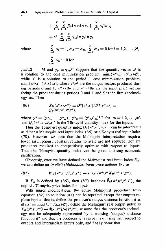
j =1,2, . . . ,M and yjk = ykj.47 Suppose that the quantity vector xo is a solution to the cost minimization problem, min,{wO*x: (yo,x)cS}, while x1 is a solution to the period 1 cost minimization problem, min,{wl*x: (yl,x)~S), where yo,yl are the output vectors produced dur- ing periods 0 and 1, wo ) ) ON and w1 ) ) ON are the input price vectors facing the producer during periods 0 and 1 and S is the firm's technol- ogy set. Then
(86)
where y* = ( Y * ~ , . . . ,Y*~[), y*,,, = (yomy1m)1/2 for m = 1,2, . . . ,M, and Q o ( ~ o , w l , ~ o , x l ) is the Tornqvist quantity index for the inputs.
Thus the Tornqvist quantity index Qo (wo,wl,xo,xl) can be interpreted as either a Malmquist real input index (86) or a Konyus real input index (70). However, we note that the Malmquist interpretation requires fewer assumptions: constant returns to scale are not required, nor are producers required to competitively optimize with respect to inputs. Thus the Tornqvist quantity index can be given a strong economic justification.
Obviously, once we have defined the Malmquist real input index XM, we can define an implicit (Malmquist) input price deflator W M as
xy (xO,xl,y* ) = D* [y * ,xl]/D* [y* ,xO] = Qo (wo,wl,xo,xl)
(87) WN(wO,wl,xO,x1,y*) = w~*x1/wO-x0 Xy(xO,xl,y*).
If Xy is defined by (86), then (87) becomes ~o(wo,wl,xo,xl), the implicit Tornqvist price index for inputs.
With minor modifications, the entire Malmquist procedure from equation (82) to equation (87) can be repeated, except that outputs re- place inputs; that is, define the producer's output distance function d as d[y,x] = minh{A: (ylA,x)~S}, define the Malmquist real output index as Y~(yO,yl,x*) 3 d[yl,x*]/d[yO,x*], assume that the producer's technol- ogy can be adequately represented by a translog (output) distance function d* and that the producer is revenue maximizing with respect to outputs and intermediate inputs only, and finally show that

464 W. E. Diewert
(88) YM(YO,Yl,X*) = d*[y1,x*]/d*[yO,x*] = Qo(PO,P~,YO,Y~)
where Qo(po,pl,yo,yl) is the Tornqvist quantity index for the outputs and the nth component of the reference input vector, X*n = ( x O ~ X ~ ~ ) ~ ' ~ ,
It = 1,2, . . . ,N.48 Thus again the Tornqvist index can be given a strong economic justification.
8.3 Methods for Justifying Aggregation over Sectors
8.3.1 Aggregation without Optimizing Behavior
Suppose there are M firms in a sector, each of which produces a single product using N inputs. Let the firm technologies be representable by means of firm production functions f", where y" = fn(xml, . . . ,x"N) denotes the amount of output producible by firm rn using input quanti- ties xml, . . . ,xmN for m = 1,2, . . . ,M. Klein's ( 1 9 4 6 ~ ) aggregation over sectors problem49 can be phrased as follows: What conditions on the firm production function's f"' will guarantee the existence of: (a ) an aggregate production function G , ( b ) input aggregator functions g1, . . . ,gN, and (c) an output aggregator function F such that the fol- lowing equation holds for a suitable set of inputs x"*~?
(89) F(Y', . . - ,y') = G[gi(xli,. - . . . , g N ( X l N , . . . ,XMN)l.
,xYi),g2(x12, . . - ,xM2),
Klein (1946b) explicitly asked that (89) hold without the assump- tion of profit-maximizing behavior by producers, since in the real world monopolistic practices may be prevalent and thus it would be pref- erable to be able to derive an aggregate production function without the assumption of competitive behavior.
Unfortunately, Nataf (1948) demonstrated that the conditions on the micro production functions f", m = 1,2, . . . ,M, that are necessary to de- rive (89) are very stringent: the fm must be strongly separable; that is, f" must have the structure fm(xml, . . . ,xmN) = h"[kml (xml) + . . . + k r n ~ ( x m N ) ] , where the hm and k", are monotonically increasing func- t i o n ~ . ~ ~
The restrictive separability assumptions on the micro production functions51 required for Klein-Nataf sectoral aggregation seem to limit the usefulness of the method from an empirical point of view.sA more promising method is outlined in the following section.
8.3.2 Aggregation with Optimizing Behavior
Bliss (1975, p. 146) notes that if all producers are competitive profit maximizers and face the same prices, then the group of producers can

465 Aggregation Problems in the Measurement of Capital
be treated as if they were a single producer subject to the sum52 of the individual production sets. Thus, if the time period is chosen to be long enough so that all inputs and outputs are variable, there is no problem of aggregation over sectors (provided producers are behaving competi- tively).
This extremely simple aggregation criterion does not seem to have been stressed very much in the literature, but it is certainly explicit in the contributions of Hotelling (1935), May (1946), Pu (1946) and Cornwall (1973, p. 512), though not stated as elegantly as the above criterion noted by Bliss.
8.3.3 Aggregation with Optimizing Behavior for Some Goods: Vintage Production Functions
Assume we have M sectors in an economy (or M firms in an industry or M plants or processes in a firm) and the production possibilities set for the mth sector is denoted by S”, m = 1,2, . . . ,M. Define the sectoral variable profit functions ll” as
(90) nm(p,X“,zm) = max,{p*y: ( y , x m , z m ) ~ S f f l ) ,
where p ) ) Ox is a vector of output (and or intermediate input) prices each sector faces for the first K goods, x” 2 ON is a vector of “labor” inputs utilized by the mth sector, and z“ is a vector of fixed “capital” inputs that could be specific to the mth sector for m = 1,2, . . . ,M. Fol- lowing Solow (1964), we could interpret the nm as being dual to the “vintage” production functions f” (of a single firm) that utilize the “vintage” capital inputs zm in addition to labor inputs xm. Assume further that the firm has a fixed vector of labor inputs x ) ) ON to allocate across the M processes. The firm will then wish to solve the following vintage or micro labor maximization problem (which defines the aggregate vari- able profit function ll) :
m = 1,2,. . . ,M,
Y
nt=l 2 xm 5 x , x m 2 O N
= ll(p,x,z1,22, . . . ,zM). (92)
A g e n e r a l i ~ e d ~ ~ Solow (1964), Fisher (1965), and Stigum (1967, 1968) vintage capital aggregation problem is: Under what condition: on the “vintage” technologies Sgfi (or nm) do there exist functions ll and g such that

466 W. E. Diewert
where g(z1,z2, , . . ,zM) can be interpreted as a capital aggregate? This problem is difficult to solve because the aggregate variable profit
function II(p,x,zl,. . . ,Zw) is not related to the micro variable profit functions IIm(p,xmzm) in any very obvious way. However, it is possible to derive a problem that is equivalent to (93) and then apply some re- sults from Gorman ( 1 9 6 8 ~ ) to the equivalent problem. Below, I indi- cate how this equivalent problem can be derived and solved.
If the firm is given a vector of positive labor prices, w ) ) ON, the firm can optimize with respect to the labor inputs. Thus define the following vintage or micro (labor optimized) variable profit functions HI*":
(94) m = 1,2,. . . ,M,
where p ) OK is the vector of output prices each sector faces for the first K goods and zm is the vector of fixed capital inputs specific to the mth sector. The (labor optimized) variable profit functions lI*" can be used to provide a complete characterization of the sectoral technol- ogies S" (under appropriate regularity conditions; see Gorman 1968a or Diewert 1 9 7 3 ~ ) just as the original variable profit functions II" can be used.
The firm or macro (labor optimized) variable profit function II* dual to II is defined as
(95)
I I * n t ( p , ~ , ~ m ) = max,{II"(p,x,z") - W * X :
x 2 O N } ,
IT*(p,w,zl, . . . ,zdJ1) E rnax,{II(p,x,zl, . . . ,zM) - W * X : x 2 O N } .
We may now state the problem that is equivalent to the original generalized Solow vintage capital aggregation problem (93) : Under what conditions on the "vintage" technologies S" (or equivalently II" or II*") do there exist functions II* and g* such that
(96)
where g*(z', . . . ,P) can be interpreted as a capital aggregate? This problem is reasonably easy to solve because the aggregate (labor
optimized) variable profit function 11* is related in a simple manner to the micro (labor optimized) variable profit functions II*".
IT* (p,w,z1, . . . ,ZW) = II*[p,w,g* (Zl, . . . ,291,
(97) Theorem: If the micro variable profit functions lIm(p,xm,zm) are concave54 and increasing in xm for m = 1,2, . . . ,M, then
M
m=1 rI*(p,w*,21,. . . ,zM) = 8 II*m(p,w*,zm),
467 Aggregation Problems in the Measurement of Capital
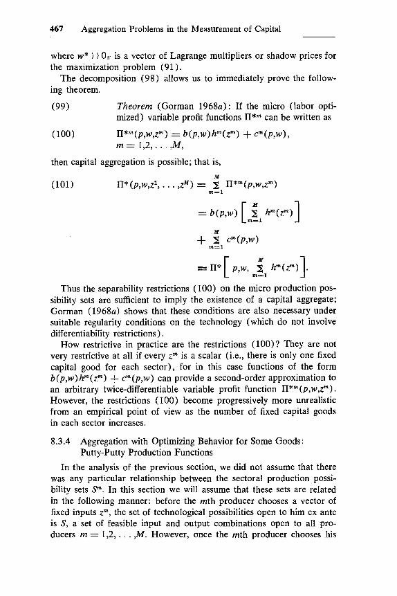
where w* ) ) 0, is a vector of Lagrange multipliers or shadow prices for the maximization problem (91 ) .
The decomposition (98) allows us to immediately prove the follow- ing theorem.
(99) Theorem (Gorman 1 9 6 8 ~ ) : If the micro (labor opti- mized) variable profit functions II*, can be written as
(100) m = 1,2,. . . ,M,
then capital aggregation is possible; that is,
n*m(P,w,Zm) = b(p,w)h"(z") + Crn(P ,W) ,
Thus the separability restrictions (100) on the micro production pos- sibility sets are sufficient to imply the existence of a capital aggregate; Gorman (1968a) shows that these conditions are also necessary under suitable regularity conditions on the technology (which do not involve differentiability restrictions).
How restrictive in practice are the restrictions (loo)? They are not very restrictive at all if every zm is a scalar (i.e., there is only one fixed capital good for each sector), for in this case functions of the form b(p,w)hm(zm) + cm(p,w) can provide a second-order approximation to an arbitrary twice-differentiable variable profit function n * m ( p , ~ , ~ m ) . However, the restrictions ( 100) become progressively more unrealistic from an empirical point of view as the number of fixed capital goods in each sector increases.
8.3.4 Aggregation with Optimizing Behavior for Some Goods: Putty-Putty Production Functions
In the analysis of the previous section, we did not assume that there was any particular relationship between the sectoral production possi- bility sets S". In this section we will assume that these sets are related in the following manner: before the mth producer chooses a vector of fixed inputs zm, the set of technological possibilities open to him ex ante is S, a set of feasible input and output combinations open to all pro- ducers m = 1,2, . . . ,M. However, once the mth producer chooses his
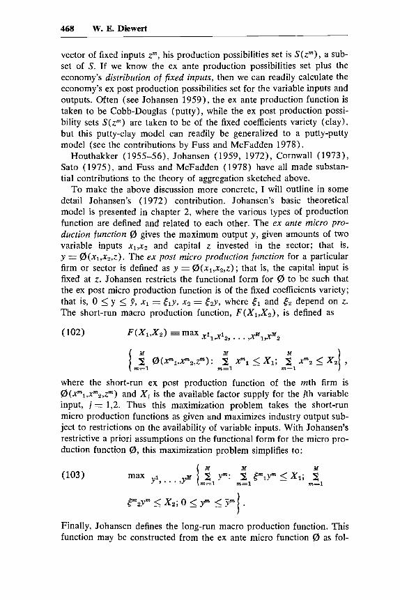
468 W. E. Diewert
vector of fixed inputs zm, his production possibilities set is S(zm), a sub- set of S . If we know the ex ante production possibilities set plus the economy's distribution of fixed inputs, then we can readily calculate the economy's ex post production possibilities set for the variable inputs and outputs. Often (see Johansen 1959), the ex ante production function is taken to be Cobb-Douglas (putty), while the ex post production possi- bility sets S(zm) are taken to be of the fixed coefficients variety (clay), but this putty-clay model can readily be generalized to a putty-putty model (see the contributions by Fuss and McFadden 1978).
Houthakker (1955-56), Johansen (1959, 1972), Cornwall (19731, Sat0 (1975), and Fuss and McFadden (1978) have all made substan- tial contributions to the theory of aggregation sketched above.
To make the above discussion more concrete, I will outline in some detail Johansen's ( 1972) contribution. Johansen's basic theoretical model is presented in chapter 2, where the various types of production function are defined and related to each other. The ex ante micro pro- duction function @ gives the maximum output y , given amounts of two variable inputs x1,x2 and capital z invested in the eector; that is, y = @(x1,x2,z). The ex post micro production function for a particular firm or sector is defined as y = @(x1,x2,z) ; that is, the capital input is fixed at z. Johansen restricts the functional form for $3 to be such that the ex post micro production function is of the fixed coefficients variety; that is, 0 5 y 2 y , xl = ,fly, x2 = f 2 y , where t1 and ,f2 depend on z. The short-run macro production function, F ( X 1 , X 2 ) , is defined as
1 A4 A4 M
m = l m = l m = l 2 JZJ(x~1,x"2,z"): 2 xml 5 XI; 2 xm2 5 XZ ,
where the short-run ex post production function of the mth firm is @(xml,xmZ,zm) and X j is the available factor supply for the jth variable input, j = 1,2. Thus this maximization problem takes the short-run micro production functions as given and maximizes industry output sub- ject to restrictions on the availability of variable inputs. With Johansen's restrictive a priori assumptions on the functional form for the micro pro- duction function @, this maximization problem simplifies to:
Ai M Y max
m=1 W % = l
P 2 Y " s xz; 0 5 y" 5 P" . 1 Finally, Johansen defines the long-run macro production function. This function may be constructed from the ex ante micro function 0 as fol-

469 Aggregation Problems in the Measurement of Capital
lows: given (variable) input-capital ratios u1 and uz, choose the opti- mal scale plant; that is, choose z so as to maximize output per unit of capital. @(ulz ,uzz ,z) /z , along a ray in input space. Denote the solution to this maximization problem as z = g ( u I , u 2 ) . Now, given aggregate amounts of inputs X 1 , X z and Z, the long-run macro production function
g(u1,u2), where u1 = X 1 / Z , u z = X 2 / Z . Note that q is homogeneous of degree one even though the micro function need not be (if Q, is linearly homogeneous, then J , = (d) .
All the production functions above can be constructed if ( a ) we know the functional form for the ex ante micro function $3 and ( b ) we know the distribution of capital stocks across firms, {z1,z2, . . . ,zM}. However, because of Johansen's assumption of no substitution between variable inputs for a fixed capital stock, he is able to combine ( a ) and ( b ) by specifying a capacity distribution { fml , (mz,ym} m = 1,2, . . . ,M for the industry, where smj is the jth input-output coefficient for the mth firm and ym is the capacity for the mth firm. From a discrete capacity distri- bution for the input-output coefficients, it is a short step to a continu- ous capacity distribution, and in Johansen ( 1972), various functional forms for continuous capacity distributions are assumed (including the case of the Pareto distribution pioneered by Houthakker, 1955-56) and the resulting macro production functions are calculated. The important conclusion that there can be considerable substitution at the macro level (even though there is none at the micro level) is emphasized by Johansen.
However, the putty-clay restrictions Johansen places on the functional form for 8 are unduly restrictive. Instead of assuming a distribution of input-output coefficients, an empirically richer and computationally simpler model would result if we assumed a "flexible" functional form for Q, (or its dual) and a multivariate distribution of fixed inputs.55 For example, let us combine output(s) and variable inputs in the vector y (where, as usual, inputs are indexed with a negative sign), let z be a vector of fixed inputs, and write the ex ante micro production function in implicit form as Q,(y,z) = 0. Let p o be a vector of variable output and input prices and define a firm's variable profit function as r ( p 0 ; z o ) = max,{po*y: +(y; zo ) = O}. Now, if T is differentiable with respect to p , it turns out that the firm's (variable) profit maximizing supply and de- mand functions, y (po; zo ) , can be obtained by differentiating r with re- spect to p;56 that is, y (po; zO) = y p ~ ( p o ; z o ) . Now suppose there are M firms in the industry and let the multivariate distribution of fixed inputs in the industry be represented by the multivariate density function f ( z ) ; that is, the number of firms having a combination of fixed factors falling
between z1 and z z is approximated by the number M J z z f(z)dz. The short-
J , is defined as J,(Xl,XZ,Z) = ~ Q , [ ~ l g ( ~ l , ~ Z ) , ~ z g ~ ~ 1 , ~ 2 ) , g(u1,uz)I/
z1
470 W. E. Diewert
run industry variable supply and demand functions Y ( p o ) can be ob- tained by integrating the firm supply and demand functions over the dis- tribution of fixed inputs; that is, Y ( p 0 ) = MJ,vpT(po; z ) f(z)dz, and the industry short-run profit function may be defined as I I ( p o > = M J d p O ; z)f(z)dz, which has as its dual the industry short-run transformation function F( Y ) = 0. The Houthakker-Johansen putty-clay assumption could be tested in this framework by assuming an appropriate func- tional form for ~ ( p ; z ) .
Unfortunately, this approach to the problem of aggregation over sectors requires ( a ) information on aggregate variable outputs and in- puts, and their prices, and ( 6 ) detailed information on the distribution of fixed inputs by firm, information that is not generally available.
This completes our discussion of the general problems of aggregation over goods and over sectors. We now turn our attention to some spe- cific problems associated with the aggregation of capital that we have not yet discussed.
8.4 The Aggregation of Capital
8.4.1 Capital: A Stock or a Flow of Services
Jorgenson and Griliches (1967, p. 257) note that: “an almost uni- versal conceptual error in the measurement of capital input is to con- fuse the aggregation of capital stock with the aggregation of capital service.” They go on to note that the aggregation procedure appropriate for measuring real investment is not appropriate for measuring real capital:
In converting estimates of capital stock into estimates of capital services we have disregarded an important conceptual error in the ag- gregation of capital services. While investment goods output must be aggregated by means of investment goods or asset prices, capital services must be aggregated by means of service prices.
The prices of capital services are related to the prices of the cor- responding investment goods; in fact, the asset price is simply the discounted value of all future capital services. Asset prices for dif- ferent investment goods are not proportional to service prices because of differences in rates of replacement and rates of capital gain or loss among capital goods. [Jorgenson and Griliches 1967, p. 2671
Thus, in the Jorgenson-Griliches framework, the user cost of capital in period t, p ! must be distinguished from the purchase cost Q t of the capital good. The easiest way of deriving the rental price p t from the purchase price Qt is to pretend that firms lease all their capital goods at rental price p t from the “leasing” firm. Competition presumably forces

471 Aggregation Problems in the Measurement of Capital
the “leasing” firm to earn the going rate of return r, after corporate in- come tax, on its leasing activities; thus we have the following equality: {purchase cost of one unit of the capital good plus corporate and prop- erty tax expenses minus rental received during the period} (1 + r ) = depreciated value of the capital good next period; in symbols we have:
(104) { Q t + u t b t - vtsQt -
xtQt1 + xtQt - ~ t } (1 + r ) =
(1 - B)Qt+i,
where ut is corporate income tax rate, vt is the proportion of depreci- ation allowable for tax purposes, 6 is the one-period combined depreci- ation and obsolescence rate for the capital good, xt is the property tax rate, and Qt+l is next period’s expected purchase price for one unit of the capital good. Now equation (104) may be solved for p t : 5 7
(105) P t = {rQt + 6Qt+i - ( Q t + i - Q t ) - (1 + r)utvtsQt
+ (1 + r ) ( l - u t ) x t Q t } / ( l + r ) (1 - ut).
If “leasing” firms do not exist, then the rental formula (105) can also be derived by setting up the firm’s profit maximization problem. For example, consider the following specific profit maximization problem:
max pvY - w ~ W - WBB - ]Qt - -Qt+i
w.r.2. Y,W,B,K 4- xtQt 1 K
subject to Y = f ( W , B , K ) , where p g is the price of one unit of output Y , ww is the white-collar wage rate, we is the blue-collar wage rate, W and B are the inputs of white- and blue-collar labor, and f is the firm’s production function. The maximand (106) can be rewritten (after some algebraic manipulations) as:
(107)
where p t is defined by (105). Thus, whether “leasing” firms exist or not, p t defined by (105) is the appropriate user cost of a unit of (corporate) capital, and it appears to be the price which should be used to weight that particular component of the capital stock K , just as py is the appropriate price to weight Y, and so on.
Once rental prices for the various components of the capital stock have been determined, the aggregation techniques discussed in sections
(1 - ut) { P ~ Y -wwW - WBB - M},
472 W. E. Diewert
8.2 and 8.3 can be used to form estimates of the aggregate stock of capital services (or components of this aggregate). This is essentially the procedure followed by Jorgenson and Griliches ( 1967).
Under the assumptions above, rental prices of capital goods can be treated symmetrically (in the theory of production and productivity analysis) to output and variable input prices. Thus it seems that the aggregation of capital is no more difficult than the aggregation of any- thing else, such as labor, intermediate goods, or output. This is the posi- tion taken by Bliss (1975, p. 144).
However, even if in theory the aggregation of capital does not appear to be any more difficult than the aggregation of say, labor, in practice it is very much more difficult to construct a capital aggregate that re- searchers can agree is appropriate for the purpose at hand.58
In the following section we will consider some of the practical diffi- culties (and points of controversy) involved in the construction of capi- tal aggregates using rental price formulas similar to (105) above. In the present section, I will attempt to relax somewhat the simplifying assump- tions that allowed us to construct the rental price formula (105).
Thus far my treatment of the capital aggregation problem has made two fundamental simplifying assumptions : ( a ) a depreciated durable good is measured in units of the undepreciated good (i.e., vintages are not distinguished), and ( b ) a durable good is assumed to evaporate or depreciate at a rate that is independent of “normal” use (and inde- pendent of the vintage of the capital good) ; specifically I have assumed a constant evaporation rare model.
Jorgenson (1965, p. 51) has argued that the assumptions above are not as restrictive as they might first appear from the viewpoint of empirical applications; but, nonetheless, since they are restrictive (cf. Feldstein and Rothschild 1974), I shall indicate how they can be re- laxed in a model where capital appears as both an input and an output.
The very general model of producer behavior that I propose to utilize was developed by J. R. Hicks in Value and Capital (1946, chap. 15; see also Malinvaud 1953; Bliss 1975).
Hicks (1946, pp. 193-94) assumes that producers make production plans at the beginning of period 1 that will extend to period n. The plan consists of a list of inputs and outputs for each period, where period 1 inputs include the firm’s existing stocks of durable equipment, distinguished by physical characteristics and vintages. Hicks thinks of period n as the period when the firm winds up its affairs and sells all its remaining durable equipment, so that the list of period n outputs will include the firm’s depreciated capital stock that will be left over at the end of the period (or at the beginning of the following period). Thus, if we assume that n = 1, the Hicksian intertemporal production model reduces to the following profit maximization model: 59

473 Aggregation Problems in the Measurement of Capital
where x = a nonnegative N1-dimensional vector of current pe- riod inputs, including the firm's beginning of the cur- rent period stocks of durable equipment.
y = a nonnegative Nz-dimensional vector of current period outputs.
z = a nonnegative N3-dimensional vector whose compo- nents represent how much durable equipment the firm will have available to it at the beginning of the follow- ing period,
p z = an N1-dimensional vector of nonnegative current period (purchase) prices for inputs.
pr = an Nz-dimensional vector of nonnegative current period prices for outputs,
pz = an N3-dimensional vector of nonnegative expected fol- lowing period prices for the firm's (depreciated) dur- able equipment.
r = the one-period interest rate at which the firm can bor- row or lend, and
S = the firm's production possibility set, which is assumed to be convex, nonempty, and closed.
We note that Hicks ( 1946, p. 230) assumes that S is smoothly convex (i.e., that the boundary of the convex set Y can be described by a twice-differentiable surface), while von Neumann (1945-46, p. 2) and Morishima (1969, pp. 29-94) assume that S is a polyhedral convex set (i.e., S can be described as the set of all convex combinations of a finite number of activities).
If producer durables evaporate at a constant rate that is independent of the firm's utilization of other inputs, then the shape of the production possibility set S will be restricted, and it is easy to see that the profit maximization model (108) reduces to a profit maximization problem similar to (106). However, in general, a firm can prolong the life (and hence the value) of its durable equipment by spending more on inputs of maintenance labor and on inputs of replacement parts. Thus we should distinguish at least two broad types of labor input: production labor and maintenance labor. Increased inputs of the first type of labor will generally lead to smaller outputs of capital equipment available at the beginning of the following period, and vice versa for maintenance labor.

474 W. E. Diewert
The model of short-run profit maximization defined by (108) is cap- able of being interpreted in several ways, depending on how narrowly capital goods are classified.
If capital goods are not distinguished according to vintage, then the dimensionality of the x and z vectors will be relatively small, and (108) reduces to a variable evaporation rate model.
If capital goods are distinguished not only according to their vintage but also by their physical condition (e.g., trucks may be classified ac- cording to how many miles they have been driven, structures may be distinguished by whether or not they have been painted recently, and so on), then the dimensionality of the x and z vectors will be enormous, and (108) may be termed a “vintage” variable evaporation rate model.
Some special cases of the very general Hicksian intertemporal model of production have appeared in the literature: ( a ) Taubman and Wilk- inson (1970) assume that the physical amount of depreciation per unit of capital per unit of time depends on an index of capital utilization; ( b ) Schworm (1977) assumes that depreciation depends on an index of capital utilization (miles driven in the case of his empirical example using truck data) and units of maintenance; while (c) Epstein (1977) actually implements a highly aggregated model based on equation (108) using aggregate United States manufacturing data, but his empiri- cal results are not very favorable to the Hicksian intertemporal model (perhaps owing to aggregation problems). On the other hand, Schworm is able to derive a formula for the rental price of capital that is similar to (105) above, except that utilization and maintenance variables also appear in the formula; but the other output and input variables pertain- ing to the firm do not appear in his formula, which makes the con- struction of rental prices for components of the capital stock much easier than in the more general Hicksian intertemporal model of pro- duction.
How can we in fact construct a capital aggregate based on the Hicksian short-run profit maximization model ( l08 ) , and how will the resulting aggregate differ from a capital services aggregate constructed by means of an index number formula using rental prices similar to (105) above as weights? In the context of the Hicksian model, it is clear that we can construct several capital aggregates that must be care- fully distinguished: ( a ) a current-period capital stock aggregate (an in- put from the viewpoint of the current period) using current-period capi- tal stock prices as weights in the aggregation procedure; ( b ) a (depreciated) following-period capital stock aggregate (an output from the viewpoint of the current period) using discounted expected follow- ing-period capital stock prices as weights; (c) a current-period invest- ment aggregate (an output) using current-period investment goods

475 Aggregation Problems in the Measurement of Capital
prices as weights in the aggregation procedure; and ( d ) a capital aggre- gate that is an aggregate of ( a ) and ( b ) where capital as an input and capital as an output are oppositely signed in the index number formula that is used. This “Hicksian” capital services aggregate60 should be comparable to the Jorgenson-Griliches capital aggregate discussed earlier, except that the assumption of constant evaporation rates is not required.
Although the Hicksian model of producer behavior and the corre- sponding capital aggregates are more appealing than the constant evaporation rate model and the Jorgenson-Griliches capital aggregate, there is a major problem in implementing the Hicksian model; that is, the necessary data do not exist at present. Data on the market value and condition of the firm’s beginning of the period holdings of durables are either: ( a ) nonexistent, ( b ) extremely aggregated, or ( c ) conven- tionally determined according to depreciation rules used for tax pur- poses.G1
I will conclude this section by considering a problem Usher raised in his introduction : Should expenditures on maintenance and repair be lumped with expenditures on capital goods? If we have enough data (and we are willing to make the necessary imputations) to implement the approach to capital aggregation based on the Hicksian model of producer behavior defined by (108), then maintenance and repair should not be lumped with capital expenditures. A similar concIusion should hold if the model is based on the constant evaporation rate model ( 106), since we would expect maintenance and repair expenditures to change 6, the depreciation rate on the existing capital stock.
8.4.2
In the previous section I may have left the impression that from a theoretical point of view constructing a capital aggregate is no more difficult than constructing a labor aggregate.62 In the present section, I will readjust this impression by cataloging some of the practical diffi- culties and sources of controversy that occur when researchers attempt to construct capital aggregates that are suitable for estimating produc- tion functions or for estimating total factor productivity.
Producer’s Expectations of Future Prices
Whether we construct a capital services aggregate using the constant evaporation rate model (equation 106) or the variable evaporation rate model (equation 108), it is necessary to estimate the producer’s ex- pectations about next period’s capital stock prices (recall the price Qt+l in eq. 105 and the expected prices p a / ( 1 + r ) in eq. 108). These expected prices are generally unobservable, and thus reasonable ana- lysts could differ widely on how to estimate them. For example, Christen- sen and Jorgenson (1969, 1970) assume that producers perfectly an-
Special Problems in the Aggregation of Capital

476 W. E. Diewert
ticipate next period’s stock prices, whereas Woodland (1972, 1975) and many othersc3 assume that producers expect current stock prices to prevail in the following period (static expectations or Hicks’s [1946, p. 2051 unitary elasticity of expectations). A third alternative (followed by Epstein 1977) is to use a forecasting model to predict next period’s asset prices based on past information about the asset prices. It seems clear that the first two methods (perfect anticipations and static ex- pectations) for forming expected prices are not generally correct, while the third alternative requires extensive econometric modeling expertise, which individual producers and accountants may not possess.
Another related difficulty must be mentioned at this point. We have been constructing aggregates under the assumption that producers are maximizing profits subjzct to their technological constraints, assuming that they are facing known prices for selling their outputs and buying their inputs. We have been assuming that there was no uncertainty in- volved in the individual producer’s profit maximization problems, and thus that their attitude toward risk and uncertainty was irrelevant. How- ever, since future-period prices of capital goods are not known with certainty, it is clear that our underlying profit maximization models (e.g., eq. 106 or 108) must be modified to incorporate producers’ atti- tudes toward risk. This leads to a great number of complication^^^ whose implications for the construction of aggregates have not been fully worked out.
The problem of modeling uncertainty is related to the problem of modeling the formation of expectations, in the sense that neither prob- lem would exist (at least in theory) if there were sufficient future and insurance markets, for then the appropriate prices could be observed in the market. However, in the absence of these markets, the analyst who wishes to construct a capital services aggregate will be forced to make an imputation or assumption about future expected prices.
Jorgenson and Griliches ( 1967) have been criticized (cf. Denison 1969, pp. 6-12; and Daly 1972, pp. 49-50) for including capital gains terms in their rental price formulas for capital services, which they use as weights in order to aggregate different components of the capital stock into a capital aggregate. However, from our rather narrow viewpoint, which concentrates on the measurement of capital in the context of pro- duction function estimation and the measurement of total factor pro- ductivity, it seems clear that the capital gains term belongs in the rental price formula-what is not as clear is the validity of the Jorgenson- Griliches perfect anticipations assumption.
Interest Rates
The rental price formula (105) and the profit maximization problems (106) and (108) in the previous section all involve an interest rate r. Which r should be used? If the firm is a net borrower, then r should be
477 Aggregation Problems in the Measurement of Capital
the marginal cost of borrowing an additional dollar for one period, while if the firm is a net lender, then r should be the one-period interest rate it receives on its last loan. In practice, r is taken to be either ( a ) an exogenous bond rate that may or may not apply to the firm under con- sideration, or ( b ) an internal rate of return. I tend to use the first alter- native, while Woodland (1972, 1975) and Jorgenson and his co- workerse5 use the second. As usual, neither alternative appears to be correct from a theoretical a priori point of view; so, again, reasonable analysts could differ on which r to use in order to construct a capital aggregate.66
Note that the appropriate interest rate is a nominal (not “real”) rate of interest: any (anticipated) inflation should be taken into account by the (anticipated) capital gains term in the user cost formula (105).
Depreciation Rates
The user-cost formula in the previous section involved a depreciation rate 6. I have already commented that, in theory, the assumption of an exogenous evaporation rate 6 is not warranted; but suppose that data limitations forced us to estimate a constant 6, or perhaps a series of 6s, { a 8 } , say, where 6, would be the one-period evaporation rate applicable to a certain component of the capital stock that was s periods old. The depreciation rates (6,) are used not only in constructing rental prices in the Jorgenson-Griliches framework, but also by other analysts in con- structing capital stock series from deflated investment series (cf. Ken- drick 1961, 1976; Denison 1974).
What depreciation rates {a,} are to be used, and how are they to be constructed? There is considerable controversy in this area, much of it being very ably reviewed by Creamer (1972, pp. 62-68). Two rela- tively extreme positions can be discerned in the literature, one used by Jorgenson and his co-workers (constant evaporation; i.e., 6, = 6 for all s) and the other used by Denison and Kendrick (one-horse-shay de- preciation; i.e., 6, = 0 for all s, except s = T when ST = 1) . Actually, Denison’s depreciation assumptions are not quite as extreme as one- horse-shay depreciation, as the following quotations indicate: 67
It is not assumed that all of the investment in a category made in a particular year disappears from the gross stock simultaneously, after expiration of the average service life. Instead more realistically, retirements are dispersed around the average service life. The Winfrey S-3 distribution is used to obtain this dispersion. [Denison 1974, pp. 53-54]
To introduce an allowance for rising maintenance expense and deterioration of capital services with the passage of time, I have adopted the following expedient. To measure input of structures and
478 W. E. Diewert
equipment I have used a weighted average of indexes of the gross stock and net stock based on straight-line depreciation, with the gross stock weighted three and the net stock one. [Denison 1974, p. 551
On the other hand, for productivity comparisons, Kendrick prefers to use one-horse-shay depreciation “in order to relate real product to the comparable real capital stock estimates on a gross basis rather than a net basis” (Kendrick 1974, p. 20), but he also constructs estimates of a net capital stock using double declining-balance depreciation.
Two questions arise with respect to assumptions made about the de- preciation, deterioration, and length of lives of components of the capi- tal stock: ( a ) Do the assumptions make much difference empirically? and ( b ) What is the empirical evidence on the appropriateness of the various assumptions?
The answer to the first question appears to be an emphatic yes. Capi- tal stocks constructed on the basis of different depreciation assumptions can differ considerably.68
Some negative empirical evidence on the validity of the constant evaporation rate form of depreciation (or declining-balance or geo- metric depreciation, as it is sometimes called) is reviewed by Feldstein and Rothschild (1974). Hulten and Wykoff (1977) utilize the theo- retical model developed by Hall (1968) to estimate economic depreci- ation for various types of structures used in the United States manu- facturing sector. They found that, in most cases, a constant geometric rate of depreciation could approximate the “true” rate of depreciation rather well, with the exception of the earliest years of the asset’s life.
Overall, one can only conclude that empirical information on de- preciation rates and lengths of lives of assets is scanty, and I can only echo the recommendations of others that governments devote more re- sources in order to obtain more information.
Treatment of Indirect Taxes
Indirect taxes in a national income accounting framework are gen- erally defined as an amalgam of taxes on outputs produced by firms (sales taxes and various excise taxes) plus taxes on various inputs (in- cluding customs duties, real and property taxes, social insurance levies, and sometimes universal pension plan levies). There has been some controversy over where these taxes should be allocated when construct- ing a capital aggregate:
The treatment of indirect taxes, property taxes, and corporate profits taxes can affect the income share of the capital-land category, and also the distribution to assets within that category. The choices of national income at market prices or factor costs for weights is in-
479 Aggregation Problems in the Measurement of Capital
fluenced by this question. This question had come earlier in a review of Solow’s book, Capital Theory and the Rate of Return, as Solow had included both indirect taxes and corporate profits taxes in esti- mating the share of income to property. [Daly 1972, p. 491
From the point of view that underlies the user-cost formula (eq. 105) (which was based on the assumption that producers competitively maxi- mize profits subject to their technological constraints), the treatment of indirect taxes seems clear: indirect taxes (such as property taxes) that fall on durable inputs shoyld be included in the user-cost formula for that input, other indirect taxes (such as Social Security payments) that fall on variable inputs should be added to the market price of those inputs, whereas indirect taxes (such as sales taxes) that fall on outputs should not be added to the market price of these outputs. The con- ceptually correct prices in the Jorgenson-Griliches framework are the output prices that reflect the revenue actually received by the firm and the input prices that reflect the actual costs paid by the firm for the use of the inputs involved in the production process.
Thus customs duties and tariffs should be added to the prices of various imported goods used by firms, but sales taxes imposed on the outputs of a firm as they are sold to households (or other nonbusiness sectors) should not be added to the firm’s selling prices. But how should we treat (intermediate good) sales taxes imposed on the outputs of a firm (1, say) as the goods are sold to another firm (2, say)? Obvi- ously the tax should not be added to the selling price of firm 1, but it should be added to the selling price of firm 1 when the good is treated as an input into firm 2.69
The Form of Business Organization The user-cost formula (105) developed in the previous section im-
plicitly assumed that the firm was an incorporated firm and thus faced the appropriate corporate tax rate. However, if the firm is not incorpo- rated, then the appropriate tax rate is the owner’s personal (marginal) tax rate, which will generally differ from the corporate rate. Thus Chris- tenson and Jorgenson (1969) construct rental prices for the components of real capital input, disaggregated by class of asset and by legal form of organization. This appears to be a worthwhile methodological inno- vation, although reasonable analysts may find fault with some of the specific details of the Christensen-Jorgenson construction.
Weighting the Components of Capital
To construct real capital input, Kendrick (1972, p. 101) and Denison (1974, p. 51) favor weighting components of the captial stock by the components share of property incomei0 while Kendrick (1976) simply adds constant-dollar components of the capital stock. None of these
480 W. E. Diewert
weights appear to agree with the user-cost weights we would obtain using formula (105), except in very restrictive circumstances: using the notation of the previous section, the suggested weights that would re- place the Jorgenson-Griliches user cost (105) are rQ, and Q t respec- tively, where Qt is the current period asset price and r is a (gross or net of depreciation) rate of return.
Since r e t and Qt do not have a depreciation term, these weights tend to be much smaller than the Jorgenson-Griliches user-cost weights, and thus measures of real factor input (see section 8.5 below) using Jorgen- son-Griliches weights tend to grow faster than Kendrick-Denison mea- sures of real factor input, since capital typically has grown faster than labor during the past century. Thus the question of which weights to use when constructing a capital services aggregate is not empirically unimportant (cf. Denison 1969 and Jorgenson and Griliches 1972).
From the viewpdint of our restrictive theoretical model of produc- tion, it seems clear that the Jorgenson-Griliches weights are to be pre- ferred over the Kendrick-Denison weights.’l
Leased versus Owned Capital in the National Accounts
There is a problem in using national income accounting data to esti- mate sectoral capital stocks that must be mentioned here.72 The prob- lem is that all rented or leased components of a firm’s capital stock appear as a primary input in the finance, insurance, and real estate sector and as an intermediate input in the firm’s sector. This creates problems when sectoral “value added” production functions are esti- mated, since the sectoral capital services input will be too Thus it would be helpful if official accounts were to provide a breakdown on which sector actually used the services of a leased component of the capital stock.
The Domain of Definition of Capital
Another fundamental problem in constructing a capital aggregate that we have not yet faced is the issue Usher raised in his introduction to this volume: Should capital be defined as an aggregate of produced means of production or as an aggregate of produced and nonproduced (natural resource) factors of production? Obviously, this is a defini- tional matter that could be decided either way. However, if we opt for the first definition of a capital aggregate and are interested in estimating aggregate production functions or explaining productivity change, then it is essential that we construct an aggregate for the noncapital, non- labor, nonproduced primary inputs (such as land and natural resources), since omitting this latter aggregate (“land”) will bias estimates of ag- gregate production functions as well as estimates of total factor pro- ductivity. This point has some applications for the current system of na-

481 Aggregation Problems in the Measurement of Capital
tional income accounting in most countries, where land (and natural resources in general) is given a very minor partly because of data limitations, but partly because researchers have focused for the most part on reproducible capital and neglected the contribution of nonre- producible resources.
A second problem with the definition of capital is that some national income accounting systems do not include inventories and goods in process as components of the capital stock. The essence of a capital good seems to be that it is a produced good, part of which lasts longer than the period under consideration. Thus, in agriculture, inventories of farm animals and feed and seed are generally large and should be in- cluded as components of the capital stock. This neglect of inventories seriously biases downward the contribution of capital in most industries. This point is well recognized, and Denison (19741, Kendrick (1976), and Christensen, Cummings, and Jorgenson (1976) all include in- ventory stocks as components of their capital stocks. However, when estimating production functions, many researchers (e.g., Woodland 1975) omit inventories as components of their capital stock series.
A final, related definitional problem has been raised by Creamer:
Capital input is typically restricted to some combination of tangible assets although every analyst knows that an enterprise requires finan- cial assets, (cash and accounts receivable) as well as tangible assets in order to function. . . . However, financial assets lead a double life- one entity’s claim is another entity’s obligation. Thus, at the level of aggregation of the national economy financial claims and obligations cancel each other, except for the net balance of international claims which have been a relatively small part of U.S. stock of capital. If this is the reason for the exclusion of financial capital, it constitutes, in my view, still another argument in favor of a disaggregative approach. [Creamer 1972, p. 601
An individual firm will generally hold an “inventory” of financial capital (or working capital, as it is sometimes called) during our Hicksian period, and the cost of holding this “inventory” is just as real a cost to the firm as a payment to labor. Aggregating across firms in the private business sector of an economy will not generally cancel out these financial claims: they will cancel only if we include households, governments, and the rest of the world in the aggregate.
That financial capital is similar to physical inventories in some sense (both represent a real cost to a firm and to the private business sector of an economy) suggests that financial capital be treated like any other durable input in our accounting framework, and that financial capital should be included in any capital services aggregate, particularly since Creamer (1972, p. 60) suggests that there may have been substantial productivity gains in the use of financial capital since 1929, at least in
482 W. E. Diewert
United States manufacturing. Unfortunately, we cannot insert financial capital into our production function as just another argument: the amount of financial capital a firm will require to produce a given out- put, given a vector of physical inputs, is simply not a well-defined quantity.
One way of proceeding would be to exclude financial capital as an input into the firm’s “physical” production function, but to include financial capital as an input (along with labor, office space, etc.) into a “transactions” technology that would have the responsibility for sell- ing the physical outputs the firm produces in its “plant” and purchasing the inputs the “plant” requires. Normal credit arrangements and pay- ment procedures could be worked into the transactions technology.
We have drifted into the domain of monetary theory, and the reader is referred to Fischer (1974) and Nagatani (1978) for further refer- ences and suggestions. At this point we can only conclude that Creamer has pointed out a serious conceptual omission from most capital aggre- gates and that it is not immediately clear how we can insert financial capital into a capital aggregate using our naive production model.
Another definitional issue with respect to the scope of a capital ag- gregate has been raised by Christensen and Jo rgen~on’s~~ inclusion of the stock of household consumer durables in their recent estimates of the capital stock. Creamer makes the following comments on their procedure:
This is a puzzling addition. . . . It is certainly inconsistent with the underlying definition of a capital good-one that is used to pro- duce other goods and services. Moreover, it is inconsistent with their own (Christensen-Jorgenson) statement that “the main analytical use of the production account is in the study of producer behavior. Reve- nue and outlay must be measured from the producer’s point of view.” . . . Moreover, the inclusion of consumer’s durables in the capital stock understates aggregate total factor productivity since the methodology of estimates is such that this sector makes no contribu- tion to prod~ctivity.?~ [Creamer 1972, p. 611
Some further comments seem warranted. Christensen and Jorgenson have included in the private production sector of an economy the “process” that converts household stocks of consumer durables into service flows. Kendrick (1976) has also added consumer durables to the capital stock, justifying the procedure as follows: “This is merely an extension of the treatment presently accorded owner-occupied resi- dential structures and may be justified by the argument cited above- that shifts in sector ownership patterns should not affect investment, capital, or the associated income estimates” (Kendrick 1976, pp. 5-6).
Thus, for some purposes the inclusion of consumer durables in a capital aggregate can be justified.’? However, since this discussion of

483 Aggregation Problems in the Measurement of Capital
capital aggregation is in the context of the estimation of total factor pro- ductivity and production function estimation for the business sector of an economy that is oriented toward maximizing private profit, I would not recommend including consumer durables in a capital aggregate, since a household’s conversion of durable stocks into flows is not gen- erally a genuine business activity.
To conclude our discussion about the domain of definition of a capital aggregate, let us examine Kendrick’s (1976) rather compre- hensive definition of the capital stock. Kendrick includes the following items in his capital stock estimates for the United States:
1. business nonhuman tangibles, consisting of structures, land, natural resources, machinery and other durable equipment, and inventory stocks used in the private business sector;
2. household nonhuman tangibles, consisting of household residential real estate, automobiles, other durable goods, and household inventories;
3. government nonhuman tangibles, consisting of government struc- tures, machinery and equipment, and public capital (such as high- way construction) ;
4. human tangibles, which are defined as outlays required to produce mature human beings (rearing costs);
5. research and development expenditures; 6. education and training expenses; 7. health and safety expenditures (one-half of all outlays for health
and safety, which reduce mortality and disability are taken as rep- resenting investment) ; and
8. mobility payments, which includes portions of unemployment in- surance benefits paid, job search and hiring expenses, and moving expenses. 78
From our narrow viewpoint, concerned with productivity and pro- duction function estimation for the private business sector of an econ- omy, we would not recommend the inclusion of any of Kendrick‘s capital stock components beyond item ( 1 ) , business nonhuman tangi- bles, since the main effect of the investments listed in items ( 3 ) to (8) is to change the prices and possibly the qualities of the inputs a private firm utilizes; but these price changes are quite consistent with our model of producer behavior and do not require any special treatment. However, we can discern three possible exceptions to the general state- ment made above.
First, if portions of the government capital stock (item 3 above) are leased to private firms, these rentals could be treated as intermediate inputs into the private sector. It would also make sense to aggregate these rentals of government capital together with the corresponding privately owned components of the business capital stock.

484 W. E. Diewert
Second, the existence of certain "free" government-provided goods such as highways creates some conceptual difficulties with our basic profit maximization problems listed in section 8.4.1. For example, consider the first profit maximization problem in section 8.4.1, modified to allow for the existence of government public goods:
(109) max (1 -ut) { p I Y - WWW - wBB - ptK}
w.r.t. Y,W,B,K
subject to Y = f ( W,B,K,R1,Rz),
where all variables have been defined in section 8.4.1 except R1 = num- ber of miles of nonfreeway road utilized by the firm and Rz = number of miles of freeway used by the firm. If f is differentiable and an interior solution to the profit maximization problem exists, Y * , W*, B*, K * , say, then the solution will satisfy the following first-order necessary condi- tions for (109):
The value of the marginal products of R1 and R2 can be defined as
(W*,B*,K*,R1,R2) = p 1 2 0 and pv aR,
(114)
respectively. Define the optimal output as Y* = f ( W*,B*,K*,Rl,RZ). If the production function exhibits constant returns to scale in all five inputs, then Euler's theorem on homogeneous functions implies
af (W*,B*,K*,Rl,Rz) = p z 2 0,
(115) pIY* = wwW* + WBB* + ptK* + p iR l+ PZRZ.
If p 1 or p 2 are positive, then the firm will capture the positive mar- ginal products of the two free inputs R 1 and R2, thus making excess profits. However, if there is free entry into the industry, new firms will enter the industry and the price of the output, pV, will tend to fall. In fact, if the production function f (W,B,K,R, ,Rz) , with R I and R2 held fixed, exhibits initially increasing returns to scale and eventual decreasing re- turns to scale in W,B,K,79 then for industry equilibrium the price of out-

485 Aggregation Problems in the Measurement of Capital
put will be close to the average cost of production; that is, the following equation should (almost) hold for an individual firm in the industry:
pgY* = wWW* + WBB" + p&*.
Equations (1 15) and (1 16) imply that the shadow prices of the two types of road, p1 and p z , should be close to zero.
With this highly simplified model in mind, we can return to our dis- cussion of whether to include certain government capital goods such as highways in a capital aggregate. The answer (from the viewpoint of the economic theory of production) appears to be yes, except that the price weights for these government capital stock components will be shadow prices whose magnitude will not generally be known. However, if we assume competitive producer behavior with free entry into each in- dustry using the public capital goods, then the price weights should be close to zero. In this case government capital goods would not show up in a capital aggregate constructed according to the index number formulas discussed in section 8.2.R0
The third possible exception to my general statement that items (2) through (8) of Kendrick's capital aggregate should not be included in a capital aggregate based on my naive economic model of producer behavior is item ( 5 ) , research and development expenditures. How- ever, I am unable to make any concrete recommendations on just how research and development expenditures should be treated when forming a capital aggregate: it depends on how R&D enters the underlying eco- nomic model upon which we base our aggregation procedures.*'
The Time Period
This discussion of capital aggregation based on the Jorgenson-Gri- liches economic model of producer behavior has thus far proceeded under the assumption that all components of the capital stock are freely variable during the period under consideration. Obviously, as we shorten our Hicksian period from, say, a decade to a week, an increas- ing number of inputs will become fixed rather than variable, and in these cases (observable) market prices should be replaced by (unob- servable) shadow prices, which equal the value of the marginal products of the fixed inputs. Since these shadow prices are not generally ob- servable, it will not generally be possible to construct capital aggre- gates based on our model of producer behavior when the time period becomes short enough to cause components of the capital stock to be- come fixed.
In view of this, one might think that capital stock aggregates based on annual data would be "better" than ones based on weekly data. This is not the case, however: the annual model of producer behavior as- sumes that all inputs are freely variable and that the prices the producer
486 W. E. Diewert
faces remain constant throughout the year when neither assumption is actually satisfied in practice, and thus neither annual nor weekly aggre- gates constructed on the basis of market data will be precisely equal to the “correct” aggregates, constructed using the appropriate shadow prices.
In section 8.7 I will discuss how to build up “annual” aggregates from “weekly” aggregates, assuming that the “weekly” aggregates have been constructed correctly from the viewpoint of our economic model of producer behavior.
Choice of Index Number Formula
Unfortunately, there is no unique solution to the index number problem. Fisher’s “ideal” index number, which employs a geometric mean of the weights from both periods in a binary comparison, is neat, but it has no more fundamental economic rationale than using either first or last period weights! [Kendrick 1972, p. 951
In section 8.2.4 I argued that there was a strong economic rationale for using Fisher’s ideal index number formula, since it is a superlative index number formula; that is, it corresponds to a flexible functional form, for the underlying production function. Moreover, we indicated that all superlative index number formulas approximate each other to the sec- ond order if changes in prices and quantities between the two periods are small, while the more commonly used Paasche or Laspeyres formulas approximate superlative indexes to the first order only.
Given that the economic justification for using a superlative index number formula seems fairly strong, should we use the fixed-base method for forming a capital aggregate, or should we compare each period with the immediately preceding period-that is, use the chain principle? In section 8.2.4 I argued for the use of the chain principle, since, if it is used, price and quantity changes should be small, and all superlative index number formulas should generate virtually the same aggregate series, so that the choice of a specific superlative index num- ber formula becomes empirically irrelevant.
To conclude this section, let me note that the construction of a capital aggregate is fraught with both theoretical and empirical diffi- culties, even taking it as given that we wish to construct an aggregate that would be used in the context of production function or productivity estimation. It appears to me that the major conceptual problems are in the determination of producer’s expectations about future prices and how to deal with the resulting uncertainty, while the major practical dif- ficulties are in the estimation of depreciation rates.
With the above difficulties firmly in mind, let us turn now to a closely related topic: how to construct estimates of total factor productivity in the context of our naive model of producer behavior.
487 Aggregation Problems in the Measurement of Capital
8.5 Capital and the Measurement of Technical Progress
8.5.1 The Measurement of Total Factor Productivity with a Separable Technology
For a brief but useful survey of the literature on the measurement of economic growth and total factor productivity, see Christensen, Cum- mings, and Jorgenson (1976).
Jorgenson and Griliches (1967, 1972, pp. 83-84) advocated the use of the Tornqvist quantity index number formula Qo (recall section 8.2.3 of this chapter) and the corresponding implicit Tornqvist price index Po in the context of the measurement of total factor productivity. In this section I repeat Diewert’s (1976, pp. 124-27) justification for their procedure.
Jorgenson and Griliches (1972) use the index number formula Q o ( p o , p l ; r o , x l ) defined in section 8.2.3 not only to form an index of real input, but also to form an index of real output. Just as the aggrega- tion of inputs into a composite input rests on the duality between unit cost and homogeneous production functions, the aggregation of outputs into a composite output can be based on the duality between unit reve- nue and homogeneous factor requirements functioms2 I will briefly out- line this latter duality.
Suppose that a producer is producing M outputs, (y1,y2, . . . ,yM) = y , and the technology of the producer can be described by a factor require- ments function, g, where g(y) = the minimum amount of aggregate in- put required to produce the vector of outputs y.83 The producer’s unit (aggregate input) revenue functions4 is defined for each price vector P 2 OM by
(1 17) r (p) = max,{p*y : g(Y) 5 1, Y 2 OM}.
Thus given a factor requirements function g, (1 17) may be used to define a unit revenue function. On the other hand, given a unit revenue function t( p ) that is a positive, linearly homogeneous, convex function for p ) ) O,u, a factor requirements function g* consistent with r may be defined for y ) )OM bys5
(118) g * ( y ) = minh{h:p*y 5 r(p)A for every p 2 0,) = mink {A: 1 5 @)A for every p 2 OM such that p - y
= 1 ) = l/max,{r(p) : p * y =1, p 2 OM}.
As usual, the translog functional form may be used to provide a second-order approximation to an arbitrary twice-diff erentiable factor requirements function. Thus, assume that g is defined (at least over the relevant range of ys) by
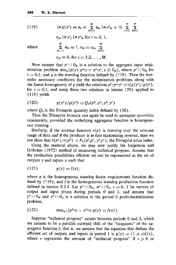
488 W. E. Diewert
cjk In y‘j In Y‘k, for r = 0, 1,
M M
where 2 am = 1, cjk = ckj , 2 m = l k=l
cjk = 0, for j = 1,2,. . . , M. Now assume that yr ) ) Oaf is a solution to the aggregate input mini-
mization problem min,{g(y) :pray = pr*yr, y 2 O M } , where p‘ ) ) OM for r = 0,1, and g is the translog function defined by (1 19). Then the first- order necessary conditions for the minimization problems along with the linear homogeneity of g yield the relations pr/p‘*y‘ = \vjg(y‘)/g(y+), for r = 0,1, and using these two relations in lemma (59) applied to (119) yields
(120)
where Qo is the Tornqvist quantity index defined by ( 3 8 ) . Thus the Tornqvist formula can again be used to aggregate quantities
consistently, provided the underlying aggregator function is homogene- ous translog.
Similarly, if the revenue function r(p) is translog over the relevant range of data and if the producer is in fact maximizing revenue, then we can show that r(pl)/r(pO) = Po(po,pl; yo,yl), the Tornqvist price index.
Using the material above, we may now justify the Jorgenson and Griliches ( 1972) method of measuring technical progress. Assume that the production possibilities efficient set can be represented as the set of outputs y and inputs x such that
g(Y1)/g(Yo) = Qo(p0, P’; YO, Y’)
(121) d Y ) = f ( x ) ,
where g is the homogeneous translog factor requirements function de- fined by (1 19), and f is the homogeneous translog production function defined in section 8.2.4. Let p‘ ? ) O J f , wr ) ) O N , r = 0, 1 be vectors of output and input prices during periods 0 and 1 , and assume that yo ) ? OM and xo ? ) ON is a solution to the period 0 profit-maximization problem,
(122) maxy,z{po*y - wO*x:g(y) = f ( x ) } .
Suppose “technical progress” occurs between periods 0 and 1, which we assume to be a parallel outward shift of the “isoquants” of the ag- gregator function f ; that is, we assume that the equation that defines the efficient set of outputs and inputs in period 1 is g(y) = (1 + T ) ~ ( x ) , where T represents the amount of “technical progress” if T > 0 or

489 Aggregation Problems in the Measurement of Capital
“technical regress” if T < 0. Finally, assume that y1 ) j OM and x1 ) ) ON is a solution to the period 1 profit-maximization problem,
(123) max, . c { ~ l * ~ - wl*x:g(y) = (1 + T)f(X)}. Thus we have g(yo) = f(xo) and g(yl) = (1 + r ) f (xl) . I t is easy
to see that y‘) ) OLM is a solution to the aggregate input minimization problem min,{g(y) : pr*y = pr*yr,y 2 Ox}, for r = 0,1, and thus (120) holds. Similarly, xr ) ) ON is a solution to the aggregator maxi- mization problem max,E{f(x) : W‘*X = wr*xr, x 2 ON}, for r = 0,1, and thus (43) holds. Substituting (43) and (120) into the identity g(yl)/g(yo) = (1 + r)f(xl)/f(xO) yields the following expression for (1 + T) in terms of observable prices and quantities:
= QO(P~,P~,Y~,Y~)/QO<W~,W~,X~,X~) - Thus the Jorgenson-Griliches method of measuring technical progress
can be justified if: ( a ) the economy’s production possibilities set can be represented by a separable transformation surface defined by g(y ) I f(x), where the input aggregator function f and the output aggregator function g are both homogeneous translog functions; (b) producers are maximizing profits; and ( c ) technical progress takes place in the “neu- tral” manner postulated above.s6
Since the separability assumption g(y) = f(x) is somewhat restrictive from an a priori theoretical point of view, it would be of some interest to devise a measure of technical progress that did not depend on this separability assumption. This can be done, as we shall see in the next section.
8.5.2 The Measurement of Total Factor Productivity in the General Case
Before analyzing a general M outputs, N inputs case, we warm up
Suppose the technology of the producer can be represented by the with the one output, N inputs case.Ri
following (time modified) translog production function f :
(125) N Y N
n = l i = l h = l lnf(x,t) = ( Y o + 2 (Yn I n xn + ?h 2 r,
x 8 P n t In xn + yr2,
n = l (YUI In xi In x h + P O t +
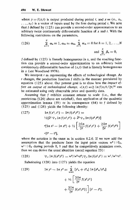
490 W. E. Diewert
where Y = f ( x , t ) is output produced during period t , and x = (XI, x2,
. . . , xN) is a vector of inputs used by the firm during period t . We note that f defined by (125) can provide a second-order approximation to an arbitrary twice continuously differentiable function of x and t . With the following restrictions on the parameters,
N
n = l and 2 Pn= 0,
f defined by (125) is linearly homogeneous in x , and the resulting func- tion can provide a second-order approximation to an arbitrary twice continuously differentiable function of (x , t ) that is linearly homogeneous in x (see Woodland 1976).
We interpret t as representing the effects of technological change. As t changes, the production function f shifts in the manner postulated by equation (125) above. Our present goal is to show how the impact ef- fect on output of technological change, T ( x , t ) =a l n f ( ~ , t ) / a t , ~ ~ can be estimated using only observable price and quantity data.
Assuming that f exhibits constant returns to scale (i.e., that the restrictions [ 1261 above are satisfied), then application of the quadratic approximation lemma (59) or its consequence (64) to f defined by (125) and (126) yields the following identity:
(127) In f(x1, t l ) - In f(x0,tO) = 1/2[9vX l n f ( x 1 , t l ) + 9'0. lnf(x0,t0)]
-[tl - to],
where the notation is the same as in section 8.2.6. If we now add the assumption that the producer faces the input price vectors wo ) ) ON, w1 ) 0s during periods 0, 1 and that he competitively minimizes costs, then we can derive the usual identities (recall equation 23) :
(128) v, In f(x0,tO) = wo/wo~Xo; v, In f (x1 , t ' ) = w'/w19x1.
Substituting (128) into (127) yields the equation N
n = l In y l - In yo = 2 [sin + SO,] In [X1,/XO,] (129)

491 Aggregation Problems in the Measurement of Capital
where yr = f ( x r , t 9 and sr, E wr, x"~/w'*x' for r = 0,l and n = 1,2, . . . , N . Equation (129) can be rearranged and exponentiated to yield the following exact relationship :
= ~ / Q o ( ~ o , w l , ~ o , x l ) , Y O
where Q o ( ~ o , ~ l , x o , ~ l ) is the Tornqvist quantity index in inputs. The left-hand side of (130) represents a theoretical expression for the cumulative effects of technical progress while the right-hand side of (130) can be calculated using observable data. If we define T' = a In f (x' , t ' ) /dt for r = 0,1, then (130) can be rewritten as
The expression (13 1 ) simplifies further if we make the additional assumption that f(x,t) = eootf(x,O), which is a strong form of Hicks's neutral technological change.s9 This assumption is equivalent to the ad- ditional restrictions on the parameters
(132) & = O , n = 1 , 2 , . . . , N a n d y = O .
With assumption ( 132), ( 13 1 ) can be rewritten as
eSort --t 1 = [ 1 (133) Y /yoI/Qo ( ~ O , w ~ , x O , x ~ ) , where Po E a In f (x , t ) /a t can be interpreted as a constant impact ef- fect of technological change.
Consider now the multiple output, multiple input case. Recall the definition of the firm's variable profit function in sections 8.2.1 and 8.2.6:
1 0
where S t r is the firm's production possibilities set at time t+, (x',y) = ( x r l , . . . , xrN, yl, . . . , yM) is a feasible vector of inputs and outputs for the firm at time tr, and p ) ) 0, is a vector of output prices at time tr.sO
Recall that the variable profit function can provide a complete de- scription of the technology of a firm under certain conditions. Now as- sume that the firm's variable profit function is the following (time modi- fied) translog function :91
(135) N A"
n = l i=l h = l In rI* (X',P',t+) = a0 + 2 a, In x'n + % 8 2
N Y
n = l m = l a h In xyi In X'h + Pot' + 2 Pn fr In + 2

492 W. E. Diewert
M M
m = l k = l 6,1nprm+'/Z 2 Z: 6mk1nprm1npry+
N Y Y
n = l m = l m=1 2 2 Enm In xrn In prm + 2 Emtr ~ ' m + ~ ( t ' ) ~ ,
where x" =_ (Y1, . . . , xrN) ) ) ON is the vector of inputs utilized by the firm at time I", and pr = ( p r , . . . , prM) ) ) Ox is the vector of output (and intermediate input) prices that the firm is facing at time tr, r = 0,l . The parameters on the right-hand side of (135) satisfy the following restrictions (which ensure that I I ( x , p , t ) is linearly homogeneous in p) :
(136) M Y
2 8 m = 1 , 6 m k = 8 k m , 2 S m y = O f o r k = l , . . . , M n C = l m = l
Y Y
m=1 m = l 2 enm = 0 for n = 1 , 2 , . . . , N a n d 8 ern = 0.
We will also assume that the firm's production is subject to constant returns to scale so that the following restrictions are also satisfied:
(137) N N
n=l i=l 3 a n = 1, ( ~ i h = a h i , 2 ( ~ i h = 0, h = 1,2 , . . . , N,
N N
n = l n = l 2 P n = 0 and 2 enrn = 0 for m = 1 ,2 , . . . , M.
If the producer is (variable) profit maximizing at time t", r = 0,1, where y r denotes the profit-maximizing vector of outputs (and inter- mediate inputs) and the producer is also cost-minimizing at time f, where w' ) ) O N denotes the vector of input prices that the producer is facing at time t', then it can be showng2 that the following equations hold :
(138) yr/pr*yr = v P In II* (xr,pr,tr) ;
wr/wr*xr = v In II* (.xr,pr,tr) ; r z 0 , l .
Note that the right-hand side of (135) is quadratic in the variables In xn, In p m , and t . Thus we can apply the quadratic approximation lemma ( 5 9 ) to (135) and obtain the following equality, which is analogous to (127) above:
(139) In II*(xl,pl,tl) - In II*(xo,po,P) x ?h [
.to veII*(xO,pO,t0) + 21 t7$ In rI*(x',p',t')]
*[lnxl- lnxo]+1/2[j1vp lnII*(xl,pl,tl) + j O
Vp II*(xo,po,tO)]*[lnpl - lnp0]

493 Aggregation Problems in the Measurement of Capital
Now define the impact effect on real value added of technological change as ~ * ( ~ , p , t ) = a In I I * ( x , p , t ) / a t . This simply a convenient way of summarizing the percentage change in real value added due to a small increment of time. In particular, define T * ~ = a In II*(xl,pl,fl)at and T * O = a In II*(xo ,p0 , to) ) /a t . Substitution of these definitions plus the relations (138) plus the identities II*(xl,pl,tl) = p l * y l and II* (xo,po, tO) = po*yo into (139) yields
After exponentiating both sides of (140), we get '1 10 1 0
(141) e1/2[T + 7 1 [t --t 1 = ~ o ( p ~ , p l , y ~ , y l ) / ~ o ( ~ ~ , ~ ~ , ~ ~ , ~ ~ ) ,
an implicit Tornqvist index of outputs divided by the Tornqvist index of inputs. Thus the right-hand side of (141) is almost identicalQ3 to the right-hand side of (124), and the Jorgenson and Griliches (1967, 1972) measure of technical progress can be (approximately) justified in the context of a general (not necessarily separable) technology.
(142) Pn = 0, n = 1,2,. . . ,N, ern = 0, m = 1,2,. . . ,M and y = 0.
Then II* ( x , p , t ) = ePot II* (x ,p ,O) = II* (xePot,p,O) ; that is, technical change is of the primary factor augmenting strongly Hicks's neutral variety. Then 7.l = T * O = PO and (141) becomes
Finally, suppose II* satisfies the additional restrictions :
(143)
Usher [1974, p. 2781 has criticized the use of the continuous time Divisia index (recall section 8.2.3) in the measurement of total factor productivity. I conclude this section by evaluating my measure of the residual (141) in the light of Usher's objections.
Usher's (1974, pp. 277-82) first objection to the Divisia index is that it will not give the correct answer unless the technology is homo- theticg4 and technical change affects the technology in a Hicks neutral manner. In my model the technology is restricted to be homothetic, since I have imposed constant returns to scale on my technology by the restrictions (137) above, and thus this part of Usher's objection applies also to my model. However, we do not require Hicks neutral tech-

494 W. E. Diewert
nological change in my model: isoquants are allowed to twist owing to technical change.
Usher’s (1974, p. 278) second objection to the Divisia index is that it is defined using time as a continuous variable but has to be computed using some sort of discrete time approximation, and that this approxi- mation will introduce errors that will possibly cumulate over time. My method of calculating the residual seems free from this defect of the Divisia index, since (141) can be evaluated as an exact equality using discrete time data. However, in reality my method is not entirely free from this criticism, since it is unlikely that my modified translog vari- able profit function n* defined by (135) could provide a very accurate approximation to the actual technology we are modeling for very long periods of time.95
Usher’s (1974, p. 278) third criticism of the Divisia index also ap- plies to my formula (141): the formula depends on the assumption that there is competitive price-taking behavior on the part of producers. However, the assumption of competitive behavior can readily be relaxed in theory: if there is monopolistic pricing behavior on the part of a producer, all we have to do is replace the observed w, p prices that occur in (141) with the appropriate marginal prices.s6 In practice this is ex- tremely difficult to do.
Usher’s (1974, p. 288) final criticism of the Divisia index methodol- ogy is more subtle than the criticisms above and deserves to be ex- tensively quoted:
The 1965 graduate is equally productive in some occupations, more productive in others, and he possesses skills that were unknown in 1940 because they depend on technology developed in the inter- vening period. The point I am making is that the relative wage of college graduates has been preserved because, and only because, technical advance has brought forth new skills and has made it profitable for people to acquire these skills, so that what we measure as labour input contains a very large component of technical change. Inputs with the same name are not the same inputs at different periods of time. . . . These considerations suggest that the use of the Divisia index coupled with the practice of treating factors of production with identical names as though they were identical factors of production may be leading us to attribute a disproportionate share of observed economic growth to the mere replication of factors of production, and may conceal the vital role of invention.
Obviously the above criticism applies with equal force to my formula (141). Of course, one method of attenuating the force of Usher’s criticism would be to treat changed inputs as new inputs. This leads us to consider the new goods problem, a problem that will be considered in section 8.6.

495 Aggregation Problems in the Measurement of Capital
Before studying the new goods problem, we will study one additional issue in the measurement of total factor productivity: the problem of defining an aggregate over sectors (or producers) measure of technical change.
8.5.3 Sectoral Estimates of Total Factor Productivity versus Economywide Measures
Domar (1961), in a classic paper,97 raised the issue of working out a method of measuring technical progress that would be invariant to the degree of aggregation and integration of processes (at the firm level), firms, industries (aggregates of firms) , and sectors (aggregates of in- dustries): "We should be free to take the economy apart, to aggregate one industry with another, to integrate final products with their inputs, and to reassemble the economy once more and possibly over different time units without affecting the magnitude of the Residual. The latter's rate of growth should, therefore, be invariant to the degree of aggrega- tion and integration and to the choice of time unit, be it a year or a decade" (Domar 1961, pp. 713-14).
Suppose we have two time periods, J sectors (or processes, or firms, or industries), and that the constant returns to scale technology of each sector can be represented by a variable profit function (which can be interpreted as a value-added function) 98 P , where
j = 1,2, . . . ,I ,
where Sit' is the jth sector's production possibilities set at time t', x'j = (xrj l , . . . , x"jNj) ) ) ONj is an N-dimensional vector of primary in-
puts used by sector j during period r, wrj = (wlrj, . . . , wrjNj) ) ) ON
is the corresponding vector of primary input prices the jth sector faces during period r, p' = (prl, . . . , prjr) ) ) O,u is the vector of positive final product (and intermediate input) prices all sectors face during period r , and yrjl, . . . , yrjlw) is the vector of outputs produced (and intermediate inputs used) by the jth sector during period r. As usual, if y'j, > 0, then the jth sector is producing the mth good during period r while if y'j, < 0, then the mth good is being utilized as an input by the jth sector during period r. Thus the components of yrj are not restricted in sign but pr*yrj > 0, since the value of outputs (minus the value of inter- mediate inputs used), pr*yrj, equals the value of primary inputs used by the jth sector during period r, wrj*xrj > 0. Note also that the primary inputs need not be the same across sectors, but that each sector faces the same output (and intermediate input) prices.
j

496 W. E. Diewert
Define the aggregate real value function II as
ll(xr1, . . . , xrJ, pr, t r ) E max,,', . . . ,,;{pro 8 y' (145) (ir, )
Thus aggregate value added is equal to the sum of sectoral value added. Define the aggregate net output vector in period r as
(147)
and define the "aggregate" vectors of inputs and input prices as
(148) x"= ( x r * , x d , . . . , x r J ) , r = 0, l
(149)
Finally, define the sectoral technical change impact coeficients dur- ing period r (assuming differentiability of the l-Ij with respect to time) as
(150)
and define the aggregate technical change impact coe@cients during period r as
(151) T " = a In II(xr,pr,tr)/at , r = 0,l.
Using (146) above, it is easy to show that the following relationship between the sectoral coefficients rrj and the aggregate technical change impact coefficient T" holds:
wr= (wrl, wr2,. . . , wrJ), r z 0,l.
T r j = a I n lTj(xr.i,pr,tr)/at, r = 0,l; j = 1,2, . . . ,I ,
J
j=1 r 2 ~ " j s'j, r = 0 3 9 1
using the definitions (150) and defining the sectoral value added shares as s"] = IIj( xrj,p",t") /II ( xr , pr,tr) = pr*yr~/pr*yr.
Recall that in section 8.5.2 I indicated that, under certain conditions, an arithmetic average of the impact coefficients % [ T O + T'] could be

497 Aggregation ProbIems in the Measurement of Capital
calculated using only observable price and quantity data. Using (152) , we see that the following relationship holds between the sectoral and aggregate average technical change coefficients:
J
j = 1 %[To + T 1 ] = ,x %[To’soi + T1’S1’]. (153)
Now suppose that for each sector the technology can be adequately represented by a sectoral translog variable profit function W* similar to the function defined by (135) , (1 36), and (137) . Then for each sector we can derive an identity similar to (141) :
1t ‘ 1 0” (154) el/2[Tof+T 1 [ t - t 1 = ~ o ( p o , p ~ , y o ~ , y ~ ~ ) /
Q , , ( W ~ ~ , W ~ ~ , ~ ~ ~ , ~ ~ ~ ) for j = 1, 2, . . . , 1.
Unfortunately, the relations (154) do not enable us to calculate the terms ‘ / Z [ T O ~ S O ~ + T1’+], which are needed to calculate the average of the aggregate technical change impact coefficients % [ T O + T 1 ] via for- mula (153) . However, if we assume that the sectoral translog variable profit functions ni* satisfy the additional restrictions similar to (142) (so that technical change is strongly Hicks neutral in each sector), then we can show, as in section 8.5.2, that
- l i - j ’ (155) - T = T for]= 1, 2 , . . . ,I ,
and the relations (1 54) can be rewritten as
(156) ‘ 1 0
e9[t --t 1 = Go (pO,pl,yoj,yli) / Q o ( W ~ ~ , W ~ ~ , X ~ J , X ~ ~ ) , j = 1 , ..., 1,
which means that the (constant) sectoral technical change coefficients can be calculated using observable price and quantity data for the two periods. Using (153) , (155), and (1561, it can be seen that the cor- rect average aggregate technical change impact coeficient ?/2 [TO + T I ]
can be calculated from observable data using the following equations :
(157)
J
j=1
= n [oo (pO,p~,yO~,yli)/Qo(~Oi,~lJ,~Oi,~li)] 1/2[8°i+81i1
E f(pO,pl,yO,yl,WO,W~,~~,x~).
0
(158)
Thus the correct aggregate measure of technical change,
+‘l] [ t l - toJ, is equal to a geometric average of the sectoral measures of
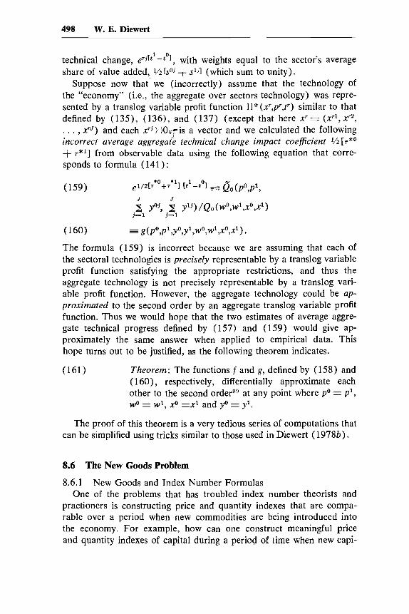
498 W. E. Diewert
1 0 technical change, eTiCt - - t 1, with weights equal to the sector’s average share of value added, Yi [sOj + s’jl (which sum to unity).
Suppose now that’ we (incorrectly) assume that the technology of the “economy” (i.e., the aggregate over sectors technology) was repre- sented by a translog variable profit function II* (xr,pr,tr) similar to that defined by (135) ’ (1361, and (137) (except that here xr= (xT1, x ~ , . . . , xrJ) and each xrj ) )OAT7 is a vector and we calculated the following incorrect average aggregate technical change impact coefficient ?4 [T*O
+ T*l] from observable data using the following equation that corre- sponds to formula (141 ) :
(159) J J
j=1 j=1 2 Y”, .x
(160) E g ( p ~ , p ~ , y ~ , y ~ , w ~ , w ~ , x ~ , x ~ ) . The formula (159) is incorrect because we are assuming that each of the sectoral technologies is precisely representable by a translog variable profit function satisfying the appropriate restrictions, and thus the aggregate technology is not precisely representable by a translog vari- able profit function. However, the aggregate technology could be up- proximated to the second order by an aggregate translog variable profit function. Thus we would hope that the two estimates of average aggre- gate technical progress defined by (157) and (159) would give ap- proximately the same answer when applied to empirical data. This hope turns out to be justified, as the following theorem indicates.
(161) Theorem: The functions f and g, defined by (158) and ( 160), respectively, differentially approximate each other to the second orderDg at any point where p o = p l , wo = wl, xo =xl and yo = yl.
The proof of this theorem is a very tedious series of computations that can be simplified using tricks similar to those used in Diewert (1978b).
8.6 The New Goods Problem
8.6.1 One of the problems that has troubled index number theorists and
practioners is constructing price and quantity indexes that are compa- rable over a period when new commodities are being introduced into the economy. For example, how can one construct meaningful price and quantity indexes of capital during a period of time when new capi-
New Goods and Index Number Formulas

499 Aggregation Problems in the Measurement of Capital
tal goods are constantly appearing on (and disappearing from) the market?
My solution to the problem is quite conventional:loO assume that the consumer (or producer) is consistently trying to solve the aggregator maximization subject to an expenditure constraint problem max,(f(x) : p' x 5 p' xr, x 2 OAT} for r = 0,l except that in period 0, when some goods are not available, the aggregator maximization problem has additional constraints imposed upon it that set the components of x = (x1,x2, . . . ,xX) that correspond to unavailable goods equal to zero.
For the sake of definiteness, let us suppose the first good is the new good that is introduced into the economy at some stage.
Obviously, if a given price and quantity are always zero, then when calculating a price or quantity index the zero good can simply be omitted from the computations. However, if a good is at a zero level during period 0 and nonzero during period 1, it is clear that the Tornqvist quantity index number formula Qo cannot be used, since the logarithm of zero is minus infinity. The Fisher quantity index Q z is well defined even if a subset of prices and quantities is zero, but we shall show below that it is not in general correct (from the viewpoint of the theory of exact index numbers) to use Q2 without some modification.
Suppose that the nonzero prices and quantities in period 0 are po2,p03, . . . , pON and xo2, xo3, . . . ,xoH, while the nonzero prices and quantities in period 1 are p l I (pll, p l ~ , . . . , p l ~ ) and xl= (xll, xlp,. . . , x l N ) respectively. We suppose that the quantity of good 1 in period 0 is xol = 0. In some circumstances we will often incorrectly assume that the price of good 1 in period 0 is also zero. However, when a new good enters the domain of our model during period 1, we should attempt to estimate the reservation price of the new good for the previous period that would rationalize the zero demand for the new good of the previous period.
Thus the theoretically correct procedure would be to form an esti- mate of the (reservation) price of good 1 in period 0, pol > 0, say, and then apply our usual index number formulas ( P z and Q 2 , say), using p" = (p01 ,p02 , . . . , p o N ) , x0 = (0, x02, . . . , xoN) and the period 1 price and quantity vectors, p' and xl . Let us denote the theoretically correct Fisher price index in the usual manner as:
(162) P2(p",p1; X 0 , X l ) = [ (p'*x"1*xl) /
(pO*xOp"*x1) 11'2.
Note that the theoretically correct index depends on the empirically unobservable price pol > 0. If we incorrectly set pol = 0 and substitute the resulting price vector into (162), we obtain the following incorrect Fisher price index (recall that xOI = 0) :

500 W. E. Diewert
Another theoretically incorrect Fisher price index could be obtained by simply ignoring good 1 for both periods; that is, set pol = p'1 = xol = xll = 0 and substitute the resulting price and quantity vectors into (162) to obtain the following index:
(164) P*2(p"p1; x0,x') = P2([0,P02, * * . , P O N I , [0,P12, * - * , pN21;
[0,x02, * . . , XONI, E0,X12,. . . ,X1NI>
The virtue of the incorrect indexes P*2 and P**, is that they may be calculated without a knowledge of the empirically unobservable PO1 > 0.
We now evaluate the bias in each of the incorrect index number formulas; that is, we take the ratio of (163) to (162) and the ratio of (164) to (162) :
where soll = pol xll/p0=x1, the share of good 1 using period 0 prices and period 1 quantities, and
and period 1 quantities.
$11 1 - = p 1 xll/pl*xl, the share of good 1 using period 1 prices
Several points immediately become apparent. ( a ) The Fisher price index P2** that incorrectly sets the price of good 1 equal to zero for period 0 is always biased upward. ( b ) The Fisher price index P*2 that incorrectly ignores the existence of good 1 for both periods need not be biased. The bias will be zero if pll/pol = pl*xl/po*xl = Pp(p0, pl;xo,xl); that is, the bias will be zero if the relative change in the price of good 1 over the two periods is equal to the general change in prices as measured by a Paasche price index. In general we would ex- pect that the relative price of good 1 would be higher in period 0 when good 1 is not yet being demanded; that is, we would expect that pll/pol 5 pl*xl/po*x', in which case

501 Aggregation Problems in the Measurement of Capital
(167) P2(p0,p1; X 0 , X 1 ) 2 P*2(p0,p1; X 0 , X 1 )
< P* * 2 (p0 ,p l ; x0,x' ) . Thus, in general P*2 will probably have a upward bias, while P**2
will definitely have a larger upward bias. Hence, in empirical applica- tions where nothing is known about the magnitude of the reservation price, pol, I would recommend the use of P*2 rather than P**, (which is sometimes used).
The quantity index corresponding to P*2 is defined by deflating the actual expenditure ratio (remember xol = 0) by P*2:
/ P * 2 (p0 ,p l ; xO,x1) = [ p l * x l / p o ~ x o ] / P * 2 (p0 ,p l ; X O , X 1 ) .
Thus the quantity index Q*2 can be calculated without a knowledge of p o l . Note that P*2 and Q * 2 are consistent with the weak factor re- versal test.
In the following section we will consider a method for obtaining empirical estimates of demand reservation prices.
8.6.2
Let us consider a slightly more general situation than the model of the previous section. We now suppose that only the first K goods to be aggregated are available in period 0 where 1 < K < N and that N goods are available in period t , t = 1, 2, . . . , T . Then the period 0 aggregator maximization problem is
(169)
A Simple Econometric Approach to the New Goods Problem
max, , 5 , . . . ,2 {f(x1,~2, . . . ,XR, 0 , . . . $1: 1 2 R
K
2 k = l
p 0 k & 5 Yo, x k 2 0, k = 1, 2, . . . , K}, where Y o > 0 is period 0 expenditure, and the period t aggregator maximization problems are
(170) max5 ,$ , . . . ,, { f (x1 ,x2 , . . . , X N > : 1 2 N
N
2 P t k X k 5 y t , X k 2 0, k = 1,2,. . . , N } ; t z 1, . . . ,T, k = l
where Yt > 0 is period t expenditure. Denote a solution to the period 0 aggregation maximization problem by the K-dimensional vector fo = (xo1,xo2, . . . , x ° K ) , and define the N-dimensional vector xo = ( x O I , X O Z ,
. . . , xoR,O, . . . ,0) = ( i 0 , O N p K ) and similarly denote period 0 prices by the K-dimensional vector bo = (po1 ,po2 , . . . , p o x ) . Denote a solution to the period t aggregation maximization problem by the N-dimensional

502 W. E. Diewert
vector xt = ( x t l , x t Z , . . . , x t N ) and define the period t price vector as
The “demand reservation prices” pOk+l, . . . ,poN are defined to be prices that “rationalize” the consumer’s or producer’s choice of xo in period 0, assuming that the new goods were available in period 0; that is, ( P O I C + ~ , PO=+^, . . . , p o N ) is a set of period 0 demand reservation (or shadow) prices if xo, a solution to (169), is also a solution to:
(171)
P t = (Ptl,Pt2, . . . ,p%) ) ) O N .
max,{f(x) : po*x 2 p0*x0, x 2 O N } ,
where Po = (PO,PO$+l, P 0 k + 2 , . . , P O X ) .
If f were differentiable at xo and we knew the functional form for f, p o could be defined by using the first-order conditions for the con- strained maximization problem ( 17 1 ) (after eliminating the Lagrange multiplier) ; that is, po/p0-xO = V,f(x0)/x0*Vf(xo) or, since po*xo = po.i.0
(172) po = (~~~~~)cl,f(x~)/x~~Vf(x~).
Thus, if the functional form for the aggregator function f were known, formula (172) could be used to estimate the “shadow” price compo- nents pOrc+l, . . . ,poN of p o = (Po, p o k + l , . . . , p o N ) = (pol, . . . , PO*,
P 0 k + l , * * * $ O N ) .
Now assume f = f r for some r > 0101 where the quadratic means of order r aggregator functions f,. were defined in section 8.2.4:
Assuming that all components of .fo are nonzero, the Kuhn-Tucker conditions for the period 0 aggregator maximization problem (169) imply :
(174) f i 0 / p * z o = V,-fr(fO, 0 , - K > / f r ( P , O N - K ) .
Similarly, assuming that all components of x1 are nonzero,1o2 the Kuhn-Tucker conditions for the period t aggregator maximization prob- lems (170) imply:
(175) p t / p t * x t = V,f , . (~~) / f , . (x~) , t = 1 , 2 , . . . , T .
Make the base period normalization :
(176) f , ( i O , O N - K ) = 1.
Now regard the system of equations defined by (174), (175), and (176) as a system of equations in the unknown aii parameters occurring in f r
defined by (173) ; that is, we are back to method I (recall section 8.2.2) for the determination of an aggregator function. The equations (174)-( 176) are particularly simple if r = 1 or r = 2. Once the para-

503 Aggregation Problems in the Measurement of Capital
meters aij that occur in the definition of f,. have been statistically deter- mined, estimated demand reservation prices for period 0 can be cal- culated using formula (172). However, in order to estimate econo- metrically the N ( N + 1) /2 aij parameters,1°3 we will require that the number of observations T + 1 be large relative to the number of goods N . In many practical situations, this condition is unlikely to be met.
8.6.3 The Hedonic Approach to the New Goods Problem
Many capital goods (e.g., trucks) came in so many varieties that it is possible to think of the good as being indexed by varying amounts x1,x2, . . . ,XN of N continuous characteristics. For example, in Griliches’s (1961) classic work,lo4 automobiles were indexed by the continuous variables horsepower, weight, and length in addition to some discrete variables. In this section I will attempt to provide a theoretical justifica- tion for Griliches’s hedonic price index approach.
Let us suppose that the producers of “trucks” can produce a truck indexed by the vector of characteristics x 3 (x1,x2, . . . , xN) in period r at a price P, . (x) equal to the minimum cost of production:
(177) P , ( x ) E C(w‘,x) ,
where C is a “truck” producer’s joint cost function, wr is a vector of input prices the truck producer faces during period r, and x is the vector of characteristics that indexes the truck, It can be shownlo5 that, under reasonable assumptions on the technology, the joint cost function C will be nondecreasing, linearly homogeneous, and concave in the input prices w, and, assuming that we are measuring characteristics so that more of a characteristic increases the cost of a truck, then C will be nondecreasing and concave in the vector x (assuming that the underly- ing technology is convex). In addition, we make the not-so-reasonable assumption that the technology is subject to constant returns to scale, so that C is linearly homogeneous with respect to x as well as w.
Another producer who uses “trucks” as an input into his productive process will want to solve the following profit maximization problem:
where uo is the number of “trucks” with characteristics x purchasedlo6 during period r at price Pp(x), u E (ul,u”) 5 (u1,uz,u3,. . . , uM) is a vector of nontruck outputs (indexed positively) and inputs (indexed negatively) produced and utilized by the producer, p r 5 (pr1,pr2, . . . , p r M ) ) ) OM is the vector of nontruck prices facing the producer during period r, and t is the producer’s transformation function.loi Note that we are assuming that characteristics enter the producer’s transformation function as uox = (uoxI, u,&, . . . , u O x N ) , the number of “trucks” pur-
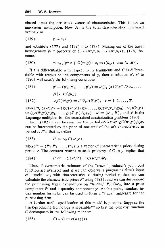
504 W. E. Diewert
chased times the per truck vector of characteristics. This is not an innocuous assumption. Now define the total characteristics purchased vector y as
(179) y 3 uox
and substitute (177) and (179) into (178). Making use of the linear homogeneity in x property of C, C(wr,x)uo = C(w',uox), (178) be- comes
(180) max,,,,{pp*u + C(wr,y) : u1 = t(ii,y), u = (ul , i)}.
If t is differentiable with respect to its arguments and C is differen- tiable with respect to the components of y, then a solution up, y' to ( 180) will satisfy the following conditions :
(181) pr = (P'l, P'2, . . . 7 P ' M ) = A'(1, a t < i r , y r > / a u 2 , *
at(u',Y'/auM) 9
.,
(182) v,C(w',y') = A' V, t($,y'), r = 1, 2, . . . , T ,
where V, C(wr,yr) = (aC(wr,y') /ayl, . . . , ~C(W' ,Y ' ) /~YM) , V,, W,Y'J = ( at(u"',y') / ay l , . . . , at (2 ,y r ) / a y N ) , ur = ( url, ii'), and A" is the Lagrange multiplier for the constrained maximization problem ( 180).
From ( 1 82) it can be seen that the partial derivative aC(w',y') /aYn can be interpreted as the price of one unit of the nth characteristic in period r , Prn; that is, define
(183)
whereP = (Prl ,Pr2, , . . , P r y ) is a vector of characteristic prices during period r. The constant returns to scale property of C in y implies that
(184)
Thus, if econometric estimates of the "truck" producer's joint cost function are available and if we can observe a purchasing firm's input of "trucks" uTo with characteristics x' during period r, then we can calculate the characteristic prices P using (1 83), and we can decompose the purchasing firm's expenditure on "trucks," P , ( x ) ur0, into a price component P' and a quantity component yr. At this point, standard in- dex number formulas can be used to form a "truck" aggregate for the purchasing firm.
A further useful specification of this model is possible. Suppose the truck-producing technology is separablelo8 so that the joint cost function C decomposes in the following manner:
(185) C(W,X) = c (w)g(x ) .
P' SES 0, c (w",y') ,
P y ' = c (w',y') = c (w',x') u',,.

505 Aggregation Problems in the Measurement of Capital
The effect of the additional assumption (185) is that a combination of cross-sectional and time-series analysis can be used to estimate the parameters of C ; that is, we can econometrically estimate the para- meters that occur in the following equation:
(186) r = 1 , 2, . . . , T ; j = 1, 2, . . . , J ,
where a, = c(w') and Pl.(xrj) = C(wr, x") is the price of a "truck" with characteristics xrj purchased by the jth firm during period r.
If, in addition, the function g in (185) can be approximated by the translog functional form, then (186) can be rewritten as (after taking logarithms of both sides) :
P,(xrj) = a,.g(x'j),
N
N N
n = l m = l + Vi 8 8 anm In xrjn In xr',
r = 1,2, . . . ,T; j = 1,2,. . . ,J , N s
n = l n = l where 2 a,= 1 , anm = am, and 8 an,= 0 for m = 1,2,. . . , N .
If we further specify that anm = 0 for all n,m, then the model defined by (187) becomes very close to Griliches's (1961) classic hedonic
prices model. However, if anm = 0 for all n,m and an > 0 with 8 a, = 1, then the function glo9 reduces to the Cobb-Douglas function that is concave in x instead of being convex in x . Thus the Griliches model cannot be obtained as a special case of our model (187), which is based on the assumption that the "truck" producer's technology is separable. However, if we assumed that the consumers of "trucks" all used a concave, linearly homogeneous, weakly separable aggregator function f in the characteristics x in order to form a "truck" aggregate f ( x ) , then instead of (186) we would obtain the model P,(x'j) = a, f ( x ' j ) , where a, can be interpreted as the price of the "truck" aggregate during period r . If we further specify f to be the translog aggregator function, we would again obtain the system of equations (187), but now the Cobb-Douglas case is perfectly consistent with this second model of producer behavior.
There are many difficulties with these theoretical treatments of the new goods problem in the context of a continuous characteristics model. However, in certain industries it should be possible to modify these models into empirically useful techniques.l1°
We have discussed the problems of aggregation over goods and ag- gregation over producers, but we have not yet discussed the problem of aggregation over time.
x
n = l
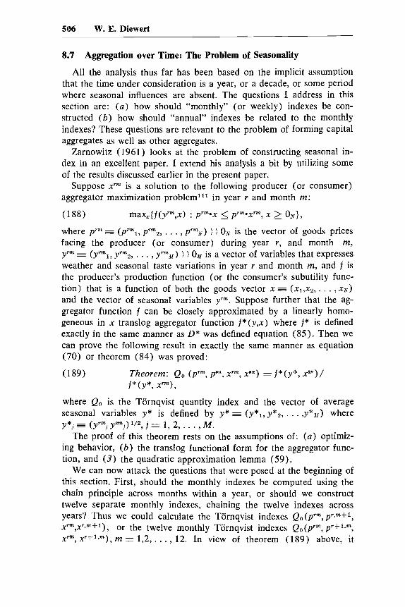
506 W. E. Diewert
8.7 Aggregation over Time: The Problem of Seasonality
All the analysis thus far has been based on the implicit assumption that the time under consideration is a year, or a decade, or some period where seasonal influences are absent. The questions I address in this section are: ( a ) how should "monthly" (or weekly) indexes be con- structed ( b ) how should "annual" indexes be related to the monthly indexes? These questions are relevant to the problem of forming capital aggregates as well as other aggregates.
Zarnowitz (1961) looks at the problem of constructing seasonal in- dex in an excellent paper. I extend his analysis a bit by utilizing some of the results discussed earlier in the present paper.
Suppose xrm is a solution to the following producer (or consumer) aggregator maximization problemlll in year r and month m:
(188)
where prm = (pml, p m z , . . . , pmX) ) ) Ox is the vector of goods prices facing the producer (or consumer) during year r, and month m, ym = (yrml, y'",, . . . , ~ ' ~ $ 1 ) ) ) 0, is a vector of variables that expresses weather and seasonal taste variations in year r and month m, and f is the producer's production function (or the consumer's subutility func- tion) that is a function of both the goods vector x 3 (xl,xZ, . . . , XN) and the vector of seasonal variables yrm. Suppose further that the ag- gregator function f can be closely approximated by a linearly homo- geneous in x translog aggregator function f*(y,x) where f* is defined exactly in the same manner as D* was defined equation (85). Then we can prove the following result in exactly the same manner as equation (70) or theorem (84) was proved:
(189) Theorem: Qo (p'", ps", xrm, xs") = f*(y*, xs")/
where Qo is the Tornqvist quantity index and the vector of average seasonal variables y* is defined by y* = ( Y * ~ , y*,, . . . ,Y*~[) where
The proof of this theorem rests on the assumptions of: ( a ) optimiz- ing behavior, ( b ) the translog functional form for the aggregator func- tion, and ( 3 ) the quadratic approximation lemma (59).
We can now attack the questions that were posed at the beginning of this section. First, should the monthly indexes be computed using the chain principle across months within a year, or should we construct twelve separate monthly indexes, chaining the twelve indexes across years? Thus we could calculate the Tornqvist indexes Qo (p'", p r ,m+l , X ~ " , X ' ~ ~ + ~ ) , or the twelve monthly Tornqvist indexes Qo (p'", p'+lvm,
xrm, x'+l,"), m = 1,2,. . . , 12. In view of theorem (189) above, it
max,{f(ym,x> : prm*x 5 pmL*xrm, x 2 O X } ,
f*(Y*, X r t n ) ,
y*j = (~'"j y5m,)1'2, j = 1, 2, . . . , M.

507 Aggregation Problems in the Measurement of Capital
seems that the latter procedure of constructing twelve monthly indexes would be better in normal circumstances, where we would expect the seasonal variables y"" to repeat themselves every twelve months. Thus, if y'" = yr+lsm, then theorem (189) tells us that we can calculate pre- cisely the ratio we are interested in, f* ( y r+ l lm, ~ ~ + l , ~ ) / f * (yrm,xrm), by evaluating the Tornqvist index, Qo(prm, pr+lpm , ¶ xrm xr+lsm), using ob- servable price and quantity data. This conclusion agrees with that reached by Hofsten and Zarnowitz, as the following quotations indicate.
This difficulty is especially obvious if seasonal fluctuations are considered. It is unnatural to accept an index which may after a year give a result different from 1, if the prices have returned to their initial values. . . . Yearly links should then be used. [Hofsten 1952, P. 271
Since 1887, when Marshall first advanced the chain system and Edgeworth seconded it, many students of index numbers have come to look upon the chain index as the standard statistical solution to changing weights. But careful consideration must be given to the question of how well chain indexes can be applied to the seasonal weight changes with whose specific features they were surely not de- signed to cope.
It is easy to demonstrate that a chain index with varying weights does not fulfill the test of proportionality (or identity). . . . Thus, on the identity test, the indexes for the same seasons should be equal, too, but they are so only for the fixed-base, not for the chain, formulae. [Zarnowitz 1961, p. 2351
Second, given that we are going to construct twelve monthly indexes, how should these indexes be related during the base year, r = O? A reasonable procedure would be to use the Tornqvist quantity index formula to construct the following eleven numbers, which could be used to compare the levels of the twelve monthly indexes during the base year: Q O ( p o m , p o - m + l 9 5 xorn xoqrn+l), rn = 1,2, . . . , 11. Theorem (189) can then be used to provide an economic interpretation of the resulting indexes. We should also note at this point (as does Zarnowitz 1961, p. 244) that the problem of disappearing goods giving rise to zero prices and quantities is particularly acute when we deal with seasonal indexes, and the reader is reminded of the discussion of the new goods prob- lem in sections 8.6.1 and 8.6.2. The techniques discussed there can also be used in the present context. Summarizing the discussion thus far, I have recommended that the chain principle across months during a base year be used to construct monthly indexes for the base year, and then the chain principle across years be used to construct twelve sep- arate monthly indexes. This procedure is of course not invariant to the

508 W. E. Diewert
choice of the base year, but in practice we would expect deviations from circularity112 to be rather small.
Finally, there is the question of how an annual index should be re- lated to the monthly indexes. In theory, the most appropriate way of forming annual aggregates would be to treat each good in each month as a separate argument in the index number formula; for example, we should compute Q,( [ p o J , . . . , p0J2], [ P I " , . . . , p1*12], [xoJ], . . . , ~ ~ v ~ ~ ] ,
[~l,', . . . , as representing the ratio of the aggregate in year 1 to year 0. However, we could apply the results on two-stage aggregation outlined in section 8.2.5 to conclude that a close approximation to the above aggregate ratio can be obtained by either ( a ) constructing monthly indexes and then aggregating these indexes over the year, or ( b ) con- structing annual indexes for each good and then aggregating over goods. The index number formula Q,, (or any other superlative quantity index) is to be used whenever an aggregate is calculated in the above two-stage procedures.
8.8 Concluding Comments
It is necessary to reemphasize that this discussion of capital aggrega- tion (and aggregation in general) has taken place in the context of production function and total factor productivity estimation, where we have consistently assumed that producers are competitively profit- maximizing or cost-minimizing or both. However, I have noted that the assumption of competitive or price taking behavior can be easily re- laxed in theory: simply replace observed prices with the appropriate marginal or shadow prices.' l a In practice, the assumption of competitive behavior will probably be required for some time yet in order to con- struct aggregates.
Given the rather narrow competitive optimizing framework, I have discussed two methods for justifying aggregation over goods such as components of the capital stock: ( a ) price pr~portionalityl'~ or Hicks's aggregation theorem (section 8.2.1 ) , and ( b ) homogeneous weak sep- arability (section 8.2.2). We have discussed a number of methods for justifying aggregation over sectors, including: (c) the method that as- sumes that all producers face the same prices with all goods (except possibly one) being freely variable during the period under consider- ation (section 8.3.2) and ( d ) a method due to Gorman ( 1 9 6 8 ~ ) and Fisher (1965) that assumes some goods are fixed but the functional forms for producer's production functions are restricted in a certain man- ner (section 8 .3 .3 ) .
In actual practice, we do not expect any of the above justifications for aggregation to hold exactly; however, we can hope that both

509 Aggregation Problems in the Measurement of Capital
methods ( a ) and (c) hold approximately at least, so that, if aggregates are used in actual applications, there is some hope that microeconomic theory will be at least approximately relevant.
I have argued that superlative index number formulas (recall section 8.2.4) should be used when aggregating over goods, assuming that there is a homogeneous weakly separable aggregator function defined over the goods in the aggregate, since superlative index number formulas correspond to flexible functional forms for aggregator functions. If the prices of the goods to be aggregated move proportionally, then the use of a superlative index number formula will also lead to the construc- tion of an aggregate that is consistent with Hicks’s aggregation theorem, even if there does not exist a homogeneous weakly separable aggregator function defined over the micro goods to be aggregated. Thus the use of a superlative index number formula is consistent with both of the gen- eral methods above for justifying aggregation over goods, and thus my first specific recommendation is that superlative indexes be used to con- struct aggregates whenever possible.
My second specific recommendation is that the chain principle be used (rather than a fixed base) whenever possible. Theoretical and practical reasons for this recommendation are scattered throughout the chapter and will not be reviewed here.
My third recommendation is that rental prices be used to weight the components of the capital stock when constructing a capital aggregate suitable for the measurement of productivity and the estimation of pro- duction functions. These rental prices should involve depreciation rates, taxes, and expectations of capital gains, although the last item presents some conceptual and practical difficulties (cf. section 8.4). However, rental prices for capital stock components need not be constructed if one employs the Hicksian view of production, which regards depreci- ated capital as a separate output.
My fourth specific recommendation is that new goods be treated in the manner outlined in section 8.6.1 when resources do not permit the implementation of the theoretically more refined techniques outlined in sections 8.6.2 and 8.6.3.
My fifth specific recommendation is that seasonaE series be constructed in the manner outlined in section 8.7; that is, roughly speaking, “sea- sonal weights” must be estimated and utilized in the construction of seasonal series.
My final recommendation is that serious consideration be given to revising the system of national accounts used in most Western countries. The basic problem with the current system is that it is not very well suited to estimating production functions or systems of consumer de- mand and labor supply functions: prices that producers face are not generally distinguished from prices consumers pay. In fact, on primary
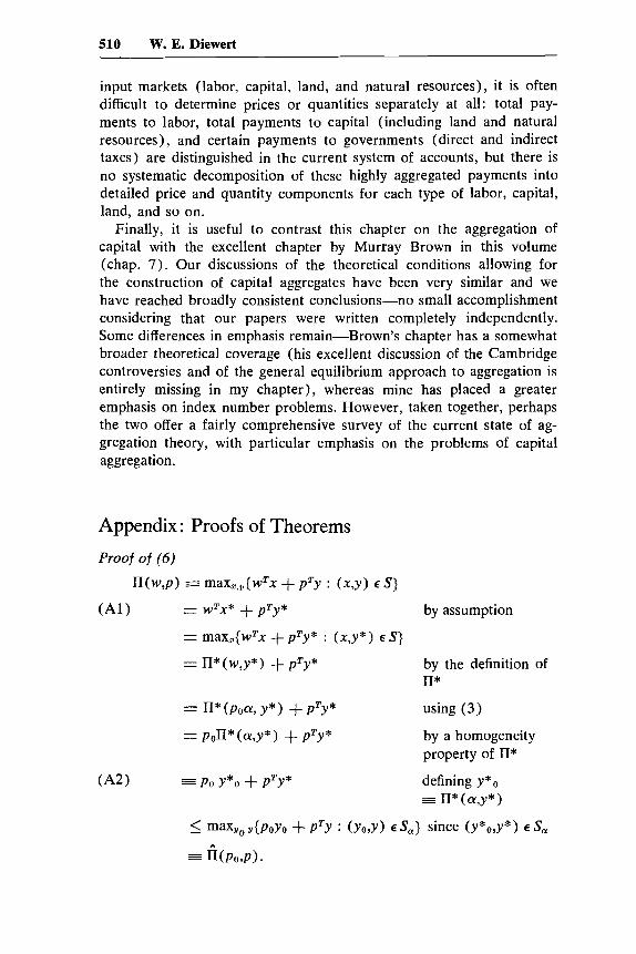
510 W. E. Diewert
input markets (labor, capital, land, and natural resources), it is often difficult to determine prices or quantities separately at all: total pay- ments to labor, total payments to capital (including land and natural resources), and certain payments to governments (direct and indirect taxes) are distinguished in the current system of accounts, but there is no systematic decomposition of these highly aggregated payments into detailed price and quantity components for each type of labor, capital, land, and so on.
Finally, it is useful to contrast this chapter on the aggregation of capita1 with the excellent chapter by Murray Brown in this volume (chap. 7). Our discussions of the theoretical conditions allowing for the construction of capital aggregates have been very similar and we have reached broadly consistent conclusions-no small accomplishment considering that our papers were written completely independently. Some differences in emphasis remain-Brown's chapter has a somewhat broader theoretical coverage (his excellent discussion of the Cambridge controversies and of the general equilibrium approach to aggregation is entirely missing in my chapter), whereas mine has placed a greater emphasis on index number problems. However, taken together, perhaps the two offer a fairly comprehensive survey of the current state of ag- gregation theory, with particular emphasis on the problems of capital aggregation.
Appendix : Proofs of Theorems
Proof of (6)
H ( w , P ) = max3,,{wTx + P'Y : (x ,Y) E S)
(A1 1 = W'X* + pTy* by assumption
= max,z{wTx + p'y* : (x,y*) E S)
= H * ( W , Y * ) + PTY*
= H*(PO% Y * ) + PTY*
= Pnn* ( a ~ * 1 + P'Y*
by the definition of rI*
using ( 3 )
by a homogeneity property of II*
Pn Y*O + P*Y* defining y*O = 11* (a , y* )

511 Aggregation Problems in the Measurement of Capital
Suppose f i ( w , ~ ) < I T ( P o , P ) = POJO + pTJ, where ( 9 0 , y ) E S,. Then J O = IT* (a,Y) = aTX for some X such that (x,J) E S
.*. II(w,p) = max,,,{poaTx + pTy : (x,y) E S}
2 PoaTx + PTJ
= P O J O + P*J
> W w , P ) ,
which is aAcontradiction, and thus our supposition is false and thus II(w,p) = I I ( p o , p ) . Note that ( A l ) = (A2) implies that = wTx*, which is equivalent to (7 ) .
Proof of (84)
The producer's technology S can be completely described by means of a transformation function t (see Diewert 1973a) : t(Y2,Y3, . . . ,YY, x1,x2, . . . ,XN) = max,,{y, : (y1,y2, . , , ,yY,xl, . . . ,xN) E S}. Further-
more, it is easy to see that if the producer has minimized the cost W*X
of producing a given vector of outputs (y1,y2, . . . ,yN), then under the usual monotonicity assumptions, the producer will also be producing the maximal amount of output 1 given that he must also produce y2, . . . ,Yr and is subject to an expenditure constraint on inputs. Thus we assume that xo is a solution to maxz{t*(y02,y03, . . . , yow,x) : WO*X = wO*XO,
x 2 ON} = yol and that x1 is a solution to max,(t* (y12, y13, . . . , Y'M, x) : wl*x = wl*xl} = yll, where t* is the firm's transformation function that corresponds to the translog distance function D*. The proof of the rest of the theorem is virtually identical to the proof of theorem (2.1 7) in Diewert (1976, pp. 139-40), except that the transformation function t*(yz,y3, . . . , yJf7 x) replaces the utility function f (x ) , and yl replaces the utility level u.
Proof of (97)
Let xl*, x2*, . . . , xu' be a solution to the maximization problem (91) . Using our assumed regularity conditions on ITrn, (91) becomes a concave programming problem, and we may apply the saddle-point theorem of Karlin (1959, p. 201) and Uzawa (1958) to obtain the existence of shadow prices w* 2 Oh', such that XI', xZ*, . . . , xY* is a solution to the following unconstrained maximization problem:
(A3 1
In fact, our strong monotonicity assumptions on IIrn (along with the concavity assumptions) imply that w* ) ) On. and that

512 W. E. Diewert
M
m = l 8 x m . = x . (A4 )
Now rewrite (A3) as
M ,....Lo
max x~
= 2 maxam Y
V b = l
,W - = 2 II*m(p,w*,z") using definitions (94).
m = l
2 x m = x , dl
m-1
1
m= 8 1 x m s x l
dl
m= 1
which is equivalent to (A3) upon defining x = 8 xrn
=max 1 M 2 rI"(p,x",z") - w**x : 5,5 I . . . ,a m = l
Y
using the monotonicity properties of rIm
= maxs{II(p,x,zl,. . . ,zM) - w*ex}
upon optimizing w.r.t. 9, . . , ,xN and using the defini- tion of II, (92)
(A61 = H*(p,w*,?, . . . , PI using the definition of II*, (95).
Thus (A5) = (A6), the desired result.
Notes
1. Notation: w ) ) 0 , means that each component of the N-dimensional vector w 3 ( w 1 , w 2 , . . . ,w,) is positive where 0, is a vector of zeros; w 2 0, means that each component is nonnegative; w > 0, means w 2 0, but wf;O,;
WTX = 8 wnxn = W * X is the inner product of the vectors w and x .
2. The only regularity condition we need impose on S is that a solution to the profit maximization problem (1 ) exist for the set of prices ( w , p ) under con-
N
n = l

513 Aggregation Problems in the Measurement of Capital
sideration. This existence will generally be assured if 5’ is a closed nonempty set with an appropriate property of boundedness from above. See McFadden (1978) or Diewert (1973a) on this point.
3. Gorman (1968a) uses this terminology. 4. McFadden (1978) and Lau (1976) use this terminology. 5. Diewert (1973a, 19746) uses this terminology. 6. See Gorman (1968a), Diewert (1973a), and Lau (1976). A property of
n* that we require below is the linear homogeneity of n* in w; that is, for every A > O , w ) ) O , , , , we have n * ( X w , y ) = A I I * ( w , y ) .
7. S is convex if and only if for every scalar such that 0 2 A 5 1 and ( x l , y l ) E S, (xz,yz) E S, we have (Ax1 + (1 - X)xZ, Ayl + ( 1 - X)yZ)c S .
8. Let 0 5 A 5 1 , ( y l , , y 1 ) E S , and ( y z 0 , y 2 ) E S,. Then y1, 2 n * ( a , y l ) and y2, 2 n*(ol ,yZ) . Convexity of S implies that n * ( a , y ) is a concave function of y (cf. Gorman 1 9 6 8 ~ ) so n*(a, Ay1 + (1 - A ) y 2 ) 2 A U * ( a , y l ) + (1 - A ) I I * (a ,y2) 2 Ayl, + (1 - A)yzo, which implies ( h y l , + (1 - A)y2,, hy l + (1 - A)Y2) E s,.
9. That is, S is a cone; if ( x , y ) E S and A 2 0, then (Ax, h y ) e S. 10. If S is a cone, then n*(h , y ) = An*(a,y) for every k 2 0, and the proof
11. See Diewert (19746, p. 139). It is an obvious modification of the translog follows readily.
function introduced by Jorgenson and Lau (1970). N Ar
z = 1 h = l
12. E E ~ = !h 2 2 pzh cth, which does not depend on r. If N = 2, then the
regularity conditions (9 ) on pzh along with the symmetry conditions pzh = phi imply that p r p l l = -p12 = -pal = p21, so that in this case E E ~ = %p[uI1 - 2uI2 + ~ ~ ~ 1 . Note that positive semidefiniteness of the variance covariance matrix [u,] implies that ull - 2uI2 + u22 2 0, so that the sign of the bias Eer is determined by the sign of p. For a general N, we could expect the bias to be small, since we would not expect a systematic correlation between p z h and u$zn.
13. The assumption of time independence is somewhat unrealistic: if the rela- tive price of the first good is higher than usual during a given period, we would expect this condition to persist for a number of subsequent periods. Thus autocor- relation is to be expected when estimating the parameters of an equation like (1 1) .
14. This terminology follows Geary and Morishima (1973). The concept of weak separability is due to Sono (1961) and Leontief (1947). Note that Shephard actually considered the problem of simultaneously aggregating x and z into two aggregates.
15. See Diewert (1974b, p. 112). Similar formulas have been derived by Chip- man ( 1970) and Samuelson ( 1972).
16. p*2’x* + w*Tz* = C*(u*; p*,w*) - - min,,,{p*Tx + w*Tz : f * ( x , z ) 2 u*} = min,,z{p*Tx + W * T Z : f [ f ( x ) , z ] 2 u * } using (14) = min,,,,y{p*Tx + W * ~ Z : f [ y , z ] 2 u*, y = f ( x ) } adding
an additional variable and equation = min,,y{c(p*)y + w*Tz : f^[y,zl 2 u*} upon minimizing
with respect to x using (17) = t ( u * ; c ( p * ) , w * ) using definition (16) = c ( p “ ) f ( x * ) + W * ~ Z * since x*,z* is a solution to the
first cost-minimization problem. 17. Proof: xr’Vf(x9 ) = f(xr) by Euler’s theorem on homogeneous functions.

514 W. E. Diewert
18. Proof: divide (26) by p r W = c(pr)f(xr). 19. If all y j k = 0, then we are in the Cobb-Douglas case and the two aggrega-
tor functions coincide. 20. Or, alternatively, assume that xr is a solution to the cost-minimization prob-
lem (17) : min,{prTx : f ( x ) 2 f ( x r ) } .
21. Solow (1957) presented his exposition in terms of a single output and two inputs. His argument is readily extended to the case of N inputs, as is done in Richter (1966), Star (1974), and Star and Hall (1976), for example.
22. Note that we do not have to estimate the unknown parameters of the pro- duction function.
23. See, for example, the empirical examples worked out in Fisher (1922). 24. See Konyus and Byushgens (1926), Afriat (1972), Pollak (1971), and
25. See Shephard (1953) or Diewert (1974b), or recall the material presented
26. Actually, we require (43) to hold only for an empirically relevant subset of
27. This theory is perhaps more clearly presented in Shephard (1953) and
28. See also Afriat (1972), Pollak (1971), Samuelson and Swamy (1974), and Diewert (1976).
29. The term is due to Lau (1974): f is a second-order differential approxi- mation to f" at the point x" if and only if f ( x 0 ) = f * ( x o ) , , V f ( x o ) = Vf*(xO) and V Z f ( x 0 ) = VZf"(x-0); that is, the levels of the functions coincide as well as their first- and second-order partial derivatives evaluated at x0. Note that V f ( x 0 )
is the vector of first-order partial derivatives of f evaluated at xo, while v * f ( x 0 ) is the matrix of second-order partial derivatives.
30. Note that VQ, stands for the vector of first-order partial derivatives of Q, with respect to all 4N arguments, etc.
31. The Laspeyres and Paasche quantity indexes give the same answer as the three "better" indexes only to the first order; that is,
Samuelson and Swamy (1974).
in section 8.2.2.
positive prices and outputs.
SO~OW (1955-56).
V2QL(p,~;x,x) # V'Qp(p#;x,+) # V'Q~(P,P;XJ). 32. The functional forms f,. and c, were studied by Denny (1974). 33. The proofs of theorems (50) and (51) do not rest on any assumption of
optimizing behavior: they are simply theorems in numerical analysis rather than economics.
34. When the chain principle is used, the limited empirical evidence in Diewert (1978b) suggests that even the Paasche and Laspeyres indexes give virtually the same answer as the superlative indexes.
35. See Shephard (1953, pp. 61-71), Solow (1955-56), Gorman (1959), Blackorby et al. (1970), and Geary and Morishima (1973, pp. 100-103).
36. We consider only the Vartia I indexes, since they are indexes that have the property of consistency in aggregation. Sat0 (19760) showed that the Vartia I1 indexes were exact for a CES aggregator function.
37. In fact, any pseudosuperlative index could be used. It is shown in Diewert ( 1978b) that any twice continuously differentiable symmetric mean of the Paasche and Laspeyres price indexes is a pseudosuperlative price index; for example, ?h P,(pO,pl; xO,xl) + ?h P p ( p o , p l ; x0,xl) is pseudosuperlative.
38. Actually, some of the components of xr can be outputs instead of inputs, in which case the corresponding components of wr are indexed with a minus sign.
39. See McFadden (1978) for the properties of these functions.

515 Aggregation Problems in the Measurement of Capital
40. The translog joint cost function is defined analogously to the translog vari- able profit function defined in section 8.2.1. However, since the logarithm of a negative number is not defined, we must renormalize the components of y s (yl, . . . , Y , ) so that each y , > 0. If y , is an intermediate input, then we renormalize the corresponding price p , to be mizus the initial positive price.
41. Diewert (19786) shows that Qo differentially approximates Qo to the sec- ond order if the partial-derivatives are evaluated at equal price and quantity vec- tors. Thus, normally, Qo(wO,wl ,xO,x~) will be numerically close to Q,(wO,wl , x 0 , x l ) . Similarly, Po will normally be close to Po.
42. We make the same sign conventions as were noted in note 40. Thus, if there are intermediate inputs, the corresponding components of p o and p l will be negative. However, Qo(pO,pl,yO,yl) can still be calculated in the usual way even if some components of p o and p l are negative.
43. We now revert back to our original sign conventions: output and input prices are all positive, as are inputs x , but components of y can be negative if the corresponding good is an (intermediate) input. Note that even if some compo- nents of yo or y l are negative, we can still calculate Po using the usual formula.
44. There is also a close correspondence with consumer surplus concepts. De- fine the consumer’s cost or expenditure function rn as r n [ f ( x ) , p ] E min,{p*x : f ( n ) 2 f ( x ) } , where f is the consumer’s utility function and p is a vector of com- modity rental prices that the consumer faces. The (Laspeyres) Allen (1949) quantity index is defined as QA(xO,xl ,pO) = rn[f(xl),po]/rn[f(xo),pl], while the (Laspeyres) Konyus (1939) cost of living index is defined as P,(pO,p*,xO)
rn [ f (xO) , p l ] / r n [ f ( x o ) ,po l . The consumer surplus concepts use arithmetic dif- ferences rather than ratios. Thus Hicks’s (1946, pp. 40-41) compensating vari- ation in income can be defined as r n [ f ( x o ) , p l ] - rn[f(xo) ,pO], while Hicks’s (1946, p. 331) equivalent variation in income can be defined as r n [ f ( x l ) , p o l
45. For formal proofs of duality theorems between distance functions and pro- duction or utility functions, see Shephard (1970), Hanoch (1978), McFadden (1978), Rockafellar (1970) and Blackorby, Primont, and Russell (1978).
46, See Gorman (1970), McFadden (1978), Hanoch (1975), and Blackorby and Russell (1976) for discussions on the separability properties of distance functions.
47. As usual, we have to change our sign conventions with respect to the components of y : assume that y = ( y l , yB, . . . , y , ) ) ) OM, but if the mth good i s actually an intermediate input, then the corresponding price p, is taken to be negative. Note that we have not restricted D * [ y , x ] to be homogeneous of degree - 1 in the components of y , which would be the case if production were subject to constant returns to scale. Finally, we note that the translog distance function can provide a second-order approximation to an arbitrary twice-differentiable distance function.
- m[f (x0) ,p03 .
48. The sign conventions of note 47 are operative here also. 49. Actually, Klein considered the problem of simultaneously aggregating over
commodities as well as sectors. 50. For an alternative proof, see Green (1964). Nataf (1948) and Green as-
sumed the f ” L were twice differentiable. These regularity conditions were relaxed by Gorman (19686) to continuity and by Pokropp (1972) to monotonicity condi- tions alone.
51. A strongly separable production function can provide only a first-order ap- proximation to a general production function.
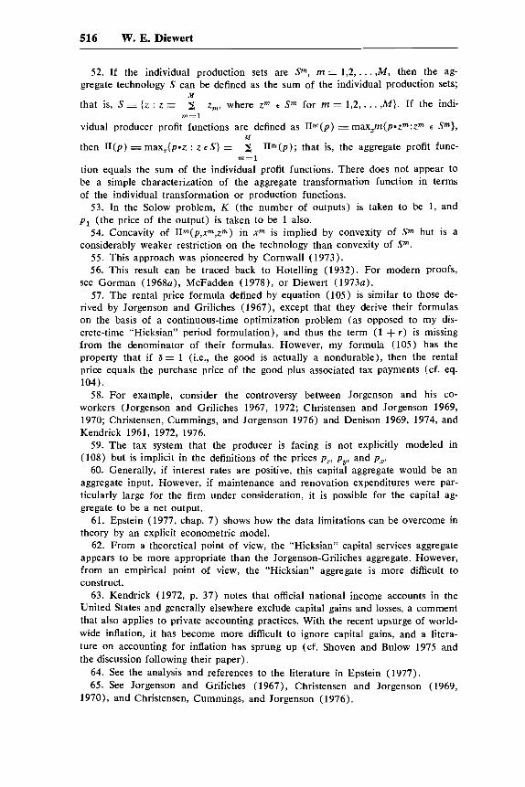
516 W. E. Diewert
52. If the individual production sets are Sm, m = 1,2,. . . ,M, then the ag- gregate technology S can be defined as the sum of the individual production sets;
that is, S = { z : z = z,, where zm E Sm for m = 1,2, . . . ,M}. If the indi-
vidual producer profit functions are defined as T l m ( p ) I maxzm{p*zn:zm E Sm>,
then II(p) n m ( p ) ; that is, the aggregate profit func-
tion equals the sum of the individual profit functions. There does not appear to be a simple characterization of the aggregate transformation function in terms of the individual transformation or production functions.
53. In the Solow problem, K (the number of outputs) is taken to be 1, and p 1 (the price of the output) is taken to be 1 also.
54. Concavity of I I n ~ ( p , x m , z m ) in xm is implied by convexity of Sm but is a considerably weaker restriction on the technology than convexity of Sm.
5 5 . This approach was pioneered by Cornwall (1973). 56. This result can be traced back to Hotelling (1932). For modern proofs,
see Gorman (1968u), McFadden (1978), or Diewert ( 1 9 7 3 ~ ) . 57. The rental price formula defined by equation (105) is similar to those de-
rived by Jorgenson and Griliches (1967), except that they derive their formulas on the basis of a continuous-time optimization problem (as opposed to my dis- crete-time “Hicksian” period formulation), and thus the term ( 1 + r ) is missing from the denominator of their formulas. However, my formula (105) has the property that if 6 = 1 (i.e., the good is actually a nondurable), then the rental price equals the purchase price of the good plus associated tax payments (cf. eq. 104).
58 . For example, consider the controversy between Jorgenson and his co- workers (Jorgenson and Griliches 1967, 1972; Christensen and Jorgenson 1969, 1970; Christensen, Cummings, and Jorgenson 1976) and Denison 1969, 1974, and Kendrick 1961, 1972, 1976.
59. The tax system that the producer is facing is not explicitly modeled in (108) but is implicit in the definitions of the prices p z , pv, and p,.
60. Generally, if interest rates are positive, this capital aggregate would be an aggregate input. However, if maintenance and renovation expenditures were par- ticularly large for the firm under consideration, it is possible for the capital ag- gregate to be a net output.
61. Epstein (1977, chap. 7 ) shows how the data limitations can be overcome in theory by an explicit econometric model.
62. From a theoretical point of view, the “Hicksian” capital services aggregate appears to be more appropriate than the Jorgenson-Griliches aggregate. However, from an empirical point of view, the “Hicksian” aggregate is more difficult to construct.
63. Kendrick (1972, p. 37) notes that official national income accounts in the United States and generally elsewhere exclude capital gains and losses, a comment that also applies to private accounting practices. With the recent upsurge of world- wide inflation, it has become more difficult to ignore capital gains, and a litera- ture on accounting for inflation has sprung up (cf. Shoven and Bulow 1975 and the discussion following their paper).
$1
8 na=l
M maxz{p*z : z E S} = 8
? ? L = l
64. See the analysis and references to the literature in Epstein (1977). 65. See Jorgenson and Griliches (1967), Christensen and Jorgenson (1969,
1970), and Christensen, Cummings, and Jorgenson (1976).

517 Aggregation Problems in the Measurement of Capital
66. The former alternative seems more plausible to me: ex post internal rates of return seem to be coo volatile to be an adequate approximation to the firm’s actual borrowing or lending rates.
67. Winfrey distributions are widely used in the construction of capital stock aggregates. However, the following quotation from Creamer (1972, p. 68) indi- cates that their empirical foundation is not strong: “An examination of Winfrey’s report discloses that the empirical basis of his distribution is his analysis of a sample of equipment retirements that are heavily weighted with railroad ties, trestles and power generating equipment. Moreover, these retirements occurred over the period 1869 and 1934. Clearly, this is an area that calls for new research.”
68. See the examples tabulated in Tice (1967) and Creamer (1972). 69. Taxes on intermediate goods could be treated as follows in a model that
aggregated firms 1 and 2: for each intermediate tax, break the corresponding com- modity up into two commodities, one of which would be the “untaxed” market where firm 1 would sell its output q at price p. The government is thought of as buying the untaxed commodity at price p and then selling it back to firm 2 on the “taxed” market price p(1 + t ) . Aggregating over the two firms would yield an aggregate “untaxed” output of q > 0 selling at price p and an aggregate “taxed” input of -q at price p(1 + f), while aggregation over the other goods could proceed as outlined in section 8.3.2. If t remained constant over time, the taxed and untaxed commodities could be aggregated using Hicks’s aggregation theorem.
70. Denison (1974) favors estimating property income nef of depreciation, whereas Kendrick (1972, p. 102) favors the net concept if one is interested in real product from a welfare standpoint, but the gross concept for production and productivity analysis.
71. The most preferred alternative would be to construct the “Hicksian” mea- sure of capital services mentioned in the previous section.
72. See Denny and Sawyer (1976) for references to the theoretical national in- come accounting literature, plus a review of current Canadian accounting prac- tices from the viewpoint of a neoclassical as opposed to a Keynesian approach to macroeconomic theory.
73. This would not be a problem if the capital services were included in sectoral estimates of intermediate inputs and gross output sectoral production functions were estimated.
74. Typically, rents to land are included in the accounting system, but asset prices and quantities of the different types of land do not appear.
75. See Christensen and Jorgenson (1969) and Christensen, Cummings, and Jorgenson (1976).
76. Creamer attributes this last point to Denison. 77. Under the appropriate assumptions, we can use the results of section 8.3.2
to justify the aggregation over the private producer sector and the household “processes” that create services out of consumer durable stocks.
78. Kendrick’s (1976, p. 15) justification for including this item is ~ v e n in the following quotation: “The costs of transfering resources are a form of in- vestment, for investment in mobility results in an increase in the future income stream beyond what incomes would be if the shifts were not made.”
79. Alternative assumptions giving the same result (item 8) are: f is linearly homogeneous, nondecreasing, and concave in all five inputs and the marginal products Bj(O,O,O,R,,R,) /aW, af(O,O,O,R,,R,) / a K exist and are finite. In this case the industry will be made up of many tiny firms each earning tiny excess profits.
80. This does not mean that government public capital is unimportant (con- sider the massive United States interstate highway system): it means that in the

518 W. E. Diewert
context of production function estimation, public capital goods should not be aggregated together with private capital but should appear as a separate inputs into the production function. However, in the context of productivity measure- ment, it does no harm to omit public capital goods, provided the shadow prices are zero, as we shall see in section 8.5.
81. Alternative economic models of R&D have recently been very ably sur- veyed by Woodland (1976).
82. See Diewert (1974a), Fisher and Shell (1972), and Samuelson and Swamy (1974) on this topic.
83. Assume g is defined for y 2 OM, and has the following yroperties: (i) g ( y ) > 0 for y ) ) 0, (positivity) (ii) g ( X y ) = h g ( y ) for x 2 0, y 2 0 (linear homo- geneity), and (iii) g ( X y l + (1 - X ) y 2 ) < Xg(y1) + (1 - A ) g ( y 2 ) for 0 < A 2 1, y l 2 OA,{, y2 2 0, (convexity).
84. If g satisfies the three properties listed in note 83, then r also has those three properties.
85. The proof is analogous to the proof of the Samuelson-Shephard duality theorem presented in Diewert (1974a); alternatively, see Samuelson and Swamy (1974).
86. A more complete exposition of the material presented in this section, with some additional material on the theory of partial Divisia indexes, can be found in Chinloy (1974).
87. The analysis for this case has been independently developed by Christen- sen, Cummings, and Jorgenson (1976), who cite Jorgenson and Lau (1979) as their source.
88. Ohta (1974) calls T the primal rate of technical progress, and he shows that it is equal to the dual rate of technical progress A defined as X = -3 In C ( y , w , t ) / a t if f exhibits constant returns to scale, where C ( y , w , f ) = minz{w*x : y = f ( x , t ) } is the producer's total cost function.
89. See Blackorby, Lovell, and Thursby (1976) for a discussion of the dif- ferent definitions of neutral technological change.
90. Make the same sign conventions as were made in the first part of section 8.2.6.
91. As usual, IT*(x,p,f) can provide a second-order approximation to an arbi- trary twice continuously differentiable n ( x , p , t ) . A special case of the time- modified translog variable profit function n* has been considered by Berndt and Wood (1975): in their model, r is a scalar output and y is a vector of inputs, SO
that, with appropriate sign changes, n* becomes a cost function. They also show under what conditions such a functional form can be consistent with factor- augmenting technical change.
92. See Diewert (1974b, pp. 137-40). 93. In Diewert (19786) it is shown that go(pO,p l , yO ,y l ) and Q o ( p o , p l , ~ o , ~ l )
approximate each other to the second order at any point where p o = p1 and YO = y l .
94. See Shephard (1953, p. 41). A production function f is homothetic if there exists a monotonically increasing function of one variable g such that g [ f ( A x ) l = h g [ f ( x ) ] for every h > 0, x 2 0,; that is, g [ f ] is linearly homogeneous.
95. The use of the chain principle should minimize this type of error: for any two consecutive time periods, tr, t r + l , we could approximate accurately the shift- ing technology of the sector by a n*T defined by (135), whose parameters depend on r.
96. This point was made by Frisch (1936) forty years ago. For more details, see Diewert (1974a, p. 155) and Appelbaum (1979).
97. Other papers on the subject include Star (1974) and Hulten ( 1978).
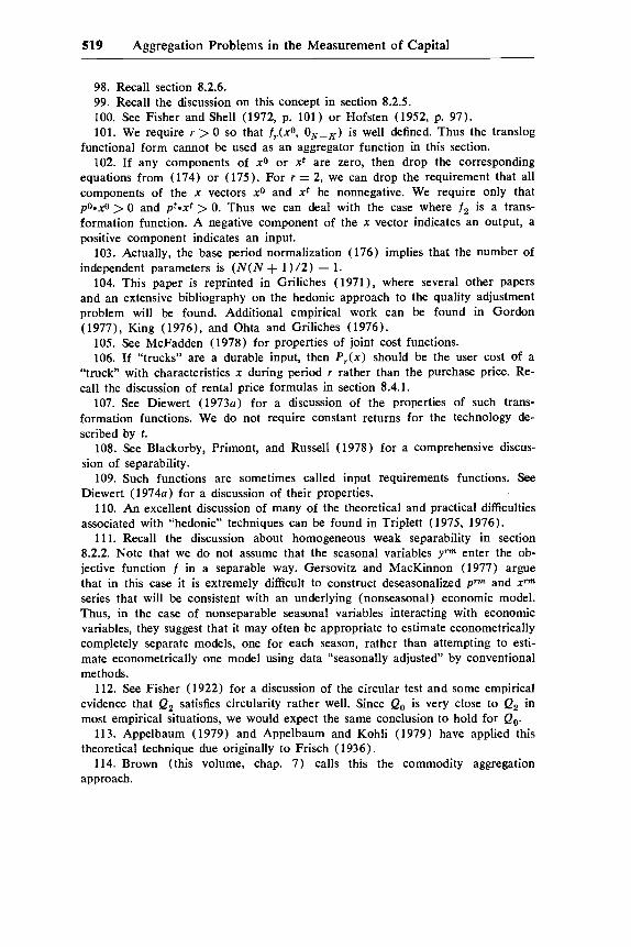
519 Aggregation Problems in the Measurement of Capital
98. Recall section 8.2.6. 99. Recall the discussion on this concept in section 8.2.5. 100. See Fisher and Shell (1972, p. 101) or Hofsten (1952, p. 97). 101. We require r > 0 so that f,.(xo, O N - K ) is well defined. Thus the translog
functional form cannot be used as an aggregator function in this section. 102. If any components of x0 or x t are zero, then drop the corresponding
equations from (174) or (175). For r = 2, we can drop the requirement that all components of the x vectors x0 and xi be nonnegative. We require only that pO*xO > 0 and pt*xt > 0. Thus we can deal with the case where f p is a trans- formation function. A negative component of the x vector indicates an output, a positive component indicates an input.
103. Actually, the base period normalization (176) implies that the number of independent parameters is ( N ( N + 1) /2 ) - 1.
104. This paper is reprinted in Griliches (1971), where several other papers and an extensive bibliography on the hedonic approach to the quality adjustment problem will be found. Additional empirical work can be found in Gordon (1977), King (1976), and Ohta and Griliches (1976).
105. See McFadden (1978) for properties of joint cost functions. 106. If “trucks” are a durable input, then P J x ) should be the user cost of a
“truck” with characteristics x during period r rather than the purchase price. Re- call the discussion of rental price formulas in section 8.4.1.
107. See Diewert (1973a) for a discussion of the properties of such trans- formation functions. We do not require constant returns for the technology de- scribed by t.
108. See Blackorby, Primont, and Russell (1978) for a comprehensive discus- sion of separability.
109. Such functions are sometimes called input requirements functions. See Diewert (1974a) for a discussion of their properties.
110. An excellent discussion of many of the theoretical and practical difficulties associated with “hedonic” techniques can be found in Triplett (1975, 1976).
11 1 . Recall the discussion about homogeneous weak separability in section 8.2.2. Note that we do not assume that the seasonal variables yrm enter the ob- jective function f in a separable way. Gersovitz and MacKinnon (1977) argue that in this case it is extremely difficult to construct deseasonalized p m and xrm series that will be consistent with an underlying (nonseasonal) economic model. Thus, in the case of nonseparable seasonal variables interacting with economic variables, they suggest that it may often be appropriate to estimate econometrically completely separate models, one for each season, rather than attempting to esti- mate econometrically one model using data “seasonally adjusted” by conventional methods.
112. See Fisher (1922) for a discussion of the circular test and some empirical evidence that Q, satisfies circularity rather well. Since Qo is very close to Q, in most empirical situations, we would expect the same conclusion to hold for Qo.
113. Appelbaum (1979) and Appelbaum and Kohli (1979) have applied this theoretical technique due originally to Frisch (1936).
114. Brown (this volume, chap. 7) calls this the commodity aggregation approach.

520 W. E. Diewert
References
Afriat, S . N. 1972. The theory of international comparisons of real in- come and prices. In International comparisons of prices and outputs, ed. D. J. Daly, pp. 13-69. New York: National Bureau of Economic Research.
Allen, R. G. D. 1949. The economic theory of index numbers. Eco- nomica, ns. , 16: 197-302.
Appelbaum, E. 1979. Testing price taking behavior. Journal of Eco- nometrics 9 283-94.
Appelbaum, E., and Kohli, U. R. 1979. Canada-United States trade: Test for the small-open-economy hypothesis. Canadian Journal of Economics 12: 1-14.
Archibald, R. B. 1977. On the theory of industrial price measurement: Output price indexes. Annals of Economic and Social Measurement
Arrow, K. J. 1974. The measurement of real value added. In Nations and households in economic growth: Essays in honor of Moses Abramovitz, ed. P. David and M. Reder. New York: Academic Press.
Bergson (Burk) , A. 1936. Real income, expenditure proportionality and Frisch’s “New methods of measuring marginal Utility.” Review of Economic Studies 4:33-52.
. 1961. National income of the Soviet Union since 1928. Cam- bridge: Harvard University Press.
Berndt, E. R., and Christensen, L. R. 1973. The translog function and the substitution of equipment, structures and labor in U.S. manufac- turing, 1929-68. Journal of Econometrics 1 : 81-1 13.
Berndt, E. R., and Wood, D. 0. 1975. Technical change, tax policy, and the derived demand for energy. Mimeographed. Department of Economics, University of British Columbia.
Blackorby, C . ; Lady, G.; Nissen, D.; and Russell, R. R. 1970. Homo- thetic separability and consumer budgeting. Economefrica 38 : 468-72.
Blackorby, C.; Lovell, D.; and Thursby, M. 1976. Extended Hicks neu- tral technical progress. Economic Journal 86: 845-52.
Blackorby, C.; Primont, D.; and Russell, R. R. 1978. Duality separabil- i ty and functional structure: Theory and economic applications. New York: American Elsevier.
Blackorby, C., and Russell, R. R. 1976. Conjugate implicit separability. Submitted to the Review of Economic Studies.
. 1978. Indices and subindices of the cost of living and the standard of living. International Economic Review 19 : 229-40.
Bliss, C . J. 1975. Capital theory and the distribution o f income. Am- sterdam: North-Holland.
6: 57-72.

521 Aggregation Problems in the Measurement of Capital
Bowley, A. L. 1928. Notes on index numbers. Economic Journal 38: 216-37.
Bruno, M. 1978. Duality, intermediate inputs and value-added. In Pro- duciton economics: A dual approach to theory and applications, vol. 2, ed. M. Fuss and D. McFadden. Amsterdam: North-Holland.
Chinloy, P. 1974. Issues in the measurement of labor input. Ph.D. diss., Harvard University.
Chipman, J. S. 1970. Lectures on the mathematical foundations of in- ternational trade theory. I. Duality of cost and production functions. Mimeographed. Vienna: Institute of Advanced Studies.
Christensen, L. R.; Cummings, D.; and Jorgenson, D. W. 1976. Eco- nomic growth, 1947-1 973 : An international comparison. Harvard Institute of Economic Research Discussion Paper 521, Harvard Uni- versity.
Christensen, L. R., and Jorgenson, D. W. 1969. The measurement of U.S. real capital input, 1929-1967. Review of Income and Wealth, ser. 15, no. 4, pp. 293-320.
. 1970. U.S. real product and real factor input, 1929-1967. Review of Income and Wealth 16, no. 1 : 19-50.
Christensen, L. R.; Jorgenson, D. W.; and Lau, L. J. 1971. Conjugate duality and the transcendental logarithmic production function. Econ- ometrica 39, no. 4:255-56.
Cornwall, R. R. 1973. A note on using profit functions to aggregate production functions. International Economic Review 14: 51 1-19.
Creamer, D. 1972. Measuring capital input for total factor productivity analysis: Comments by a sometime estimator. Review of Income and Wealth, 18, pp. 55-78.
Daly, D. J. 1972. Combining inputs to secure a measure of total factor input. Review of Income and Wealth, ser. 18, pp. 27-53.
Denison, E. F. 1969. Some major issues in productivity analysis: An examination of estimates by Jorgenson and Griliches. Survey of Cur- rent Business 49, no. 5 , part 2:l-27.
. 1974. Accounting for United States economic growth 1929- 1969. Washington, D.C. : Brookings Institution.
Denny, M. 1974. The relationship between functional forms for the production system. Canadian Journal of Economics 7 : 2 1-3 1.
Denny, M. G. S., and Sawyer, J. A. 1976. Revising,the national ac- counts. Canadian Journal of Economics 9 :720-32.
Diewert, W. E. 1971. An application of the Shephard duality theorem: A generalized Leontief production function. Journal of Political Econ- omy 79:481-507.
. 1973a. Functional forms for profit and transformation func- tions. Journal of Economic Theory 6 : 284-3 16.

522 W. E. Diewert
. 1973b. Afriat and revealed preference theory. Review of ECO- nomic Studies 40:419-26.
. 1974a. Functional forms for revenue and factor requirements functions. International Economic Review 15 : 119-30.
. 1974b. Applications of duality theory. In Frontiers of quanti- tative economics, vol. 2, ed. M. D. Intriligator and D. A. Kendrick. Amsterdam : North-Holland.
. 1976. Exact and superlative index numbers. Journal of Econo- metrics 4 : 1 15-45.
. 1978a. Hicks’ aggregation theorem and the existence of a real value added function. In Production economics: A dual approach to theory and applications, ed. M. Fuss and D. McFadden, pp. 17-51. Amsterdam: North Holland.
. 1978b. Superlative index numbers and consistency in aggrega- tion. Econometrica 46: 883-900.
Divisia, F. 1926. L’indice mone‘taire et la thtorie de la monnaie. Paris: SociCtC Anonyme du Recueil Sirey.
Domar, E. D. 1961. On the measurement of technological change. Economic Journal 7 1 : 709-29.
Epstein, L. E. 1977. Essays in the economics of uncertainty. Ph.D. diss. University of British Columbia, Vancouver.
Feldstein, M. S., and Rothschild, M. 1974. Towards an economic theory of replacement investment. Econometrica 42: 393-424.
Fischer, S. 1974. Money and the production function. Economic In- quiry 12:517-33.
Fisher, F. M. 1965. Embodied technical change and the existence of an aggregate capital stock. Review of Economic Studies 32 : 263-88.
Fisher, F. M., and Shell, K. The economic theory of price indices. New York: Academic Press.
Fisher, I. 1922. The making of index numbers. Boston: Houghton Mifflin.
Frisch, R. 1936. Annual survey of general economic theory: The prob- lem of index numbers. Econometrica 4 : 1-39.
Fuss, M., and McFadden, D. eds. 1978. Production economics: A dual approach to theory and applications. Amsterdam: North-Holland.
Geary, P. T., and Morishima, M. 1973. Demand and supply under separability. In Theory of demand: Real and monetary, ed. M. Morishima and others. Oxford: Clarendon Press.
Gersovitz, M., and MacKinnon, J. G. 1977. Seasonality in regression: Economic theory and econometric practice. Discussion Paper 257, Queen’s University, Kingston, Canada.
Gordon, R. J. 1977. The measurement of durable goods prices. New York: National Bureau of Economic Research. Forthcoming.

523 Aggregation Problems in the Measurement of Capital
Gorman, W. M. 1953. Community preference fields. Econometrica
. 1959. Separable utility and aggregation. Econometrica 27: 469- 81.
. 1968a. Measuring the quantities of fixed factors. In Value, capital and growth: Papers in honour of Sir John Hicks, ed. J. N. Wolfe, pp. 141-72. Chicago: Aldine.
. 19686. The structure of utility functions. Review of Economic Studies 35:367-90.
. 1970. Quasi-separable preferences, costs and technologies. Mimeographed. London School of Economics and Political Science.
Green, H. A. J. 1964. Aggregation in economic analysis: An intro- ductory survey. Princeton, N. J. : Princeton University Press.
Griliches, Z. 1961. Hedonic price indexes for automobiles: An econo- metric analysis of quality change. In The price statistics of the federal government. New York: National Bureau of Economic Research.
-- , Price indexes and quality change: Studies in new methods of measurement. Cambridge, Mass. : Harvard University Press.
Hall, R. 1968. Technical change and capital from the point of view of the dual. Review of Economic Studies 35:35-46.
Hanoch, G. 1975. Production or demand models with direct or indirect implicit additivity. Econometrica 43 : 395-420.
. 1978. Symmetric duality and polar production functions. In Production economics: A dual approach to theory and applications, ed. M. Fuss and D. McFadden, 1 : 113-31. Amsterdam: North Hol- land.
Hardy, G. H.; Littlewood, J. E.; and Polya, G. 1934. Inequalities. Cam- bridge: Cambridge University Press.
Hicks, John R. 1946. Value and capital. 2d ed. Oxford: Clarendon Press.
21 : 63-80.
. 1965. Capital and growth. Oxford: Oxford University Press. Hofsten, E. v. 1952. Price indexes and quality changes. London: George
Allen and Unwin. Hotelling, H. 1932. Edgeworth’s taxation paradox and the nature of
demand and supply functions. Journal of Political Economy 40: 577- 616.
. 1935. Demand functions with limited budgets. Econometrica
Houthakker, H. S. 1955-56. The Pareto distribution and the Cobb- Douglas production function in activity analysis. Review of Economic Studies 23 : 27-3 1.
Hulten, C. R. 1973. Divisia index numbers. Econometrica 41 : 1017-26. . 1978. Growth accounting with intermediate inputs. Review of
3: 66-78.
Economic Studies 45 : 5 1 1-1 8.
524 W. E. Diewert
Hulten, C. R., and Wykoff, F. C. Economic depreciation and the tax- ation of structures in U.S. manufacturing industries: An empirical analysis. Discussion Paper 77-02, Department of Economics, Uni- versity of British Columbia.
Johansen, L. 1959. Substitution vs. fixed production coefficients in the theory of economic growth: A synthesis. Econometrica 27: 157-76.
. 1972. Production functions. Amsterdam: North-Holland. Jorgenson, D. W. 1965. Anticipations and investment behavior. In The
Brookings Quarterly econometric model of the United States, ed. James S . Duesenberry and others, pp. 35-94. Chicago: Rand MC- Nally.
. 1966. The embodiment hypothesis. Journal of Political Econ- omy 74:l-17.
Jorgenson, D. W., and Griliches, Z. 1967. The explanation of pro- ductivity change. Review o f Economic Studies 34: 249-83.
. 1972. Issues in growth accounting: A reply to Edward F. Denison. Survey of Current Business 52, no. 5 , part 2: 65-94.
Jorgenson, D. W., and Lau, L. J. 1970. The transcendental logarithmic utility function and demand analysis. Department of Economics, Harvard University.
. 1979. Duality and technology. Amsterdam: North-Holland. Forthcoming.
Karlin, S . 1959. Mathematical methods and theory in games, program- ming and economics. vol. 1, Palo Alto: Addison-Wesley.
Kendrick, J. W. 1961. Productivity trends in the United States. Prince- ton: Princeton University Press.
. 1972. Economic accounts and their uses. New York: McGraw- Hill.
. 1976. The formation and stocks of total capital. New York: National Bureau of Economic Research.
Khang, C. 1971. An isovalue locus involving intermediate goods and its applications to the pure theory of international trade. Journal of International Economies 1 : 3 1 5-25.
King, A. T. 1976. The demand for housing: Integrating the roles of journey-to-work, neighborhood quality and prices. In Household production and consumption, ed. N. E. Terleckyj, pp. 451-83. New York: National Bureau of Economic Research.
Klein, L. R. 1946a. Macroeconomics and the theory of rational be- havior. Econometrica 14: 93-108.
. 19466. Remarks on the theory of aggregation. Econometrica 14: 303-12.
Kloek, T. 1967. On quadratic approximations of cost of living and real income index numbers. Report 67 10, Econometric Institute, Nether- lands School of Economics. Mimeographed.
525 Aggregation Problems in the Measurement of Capital
Konus [Konyus], A. A. 1939. The problem of the true index of the cost of living. Econometrica 7:lO-29. (Translation of a paper first published in Ekonomicheskii Byulleten Konyunkturnovo Znstituta 3 [1924]:64-71.)
Konyus, A. A., and Byushgens, S. S. 1926. K probleme pokupatelnoi cili deneg. Voprosi Konyunkfuri 2: 15 1-72.
Lau, L. J. 1974. Comments on applications of duality theory. In Frontiers of quantitative economics, ed. M. D. Intriligator and D. A. Kendrick, 2: 176-99. Amsterdam: North-Holland.
. 1976. A characterization of the normalized restricted profit function. Journal of Economic Theory 12: 131-63.
. 1979. On exact index numbers. Review of Economics and Statistics 61 :73-82.
Leontief, W. W. 1947. Introduction to a theory of the internal structure of functional relationships. Econometrica 15 : 361-73.
McFadden, D. 1978. Cost, revenue and profit functions. In Production economics: a dual approach to theory and applications. eds. M. Fuss and D. McFadden, 1 : 3-1 09. Amsterdam-North-Holland.
Malinvaud, E. 1953. Capital accumulation and the efficient allocation of resources. Econometrica 21 : 233-68.
Malmquist, S. 1953. Index numbers and indifference surfaces. Trabajos de Estadistica 4: 209-42.
May, K. 1946. The aggregation problem for a one-industry model. Econometrica 14 : 285-9 8.
Moorsteen, R. H. 1961. On measuring productive potential and rela- tive eficiency. Quarterly Journal of Economics 75 :451-67.
Morishima, M. 1969. Theory of economic growth. London: Oxford University Press.
Nagatani, K. 1978. Monetary theory, Amsterdam: North-Holland. Nataf, A. 1948. Sur la possibilitk de construction de certains macro-
modkles. Econometrica 16: 232-44. Neumann, J. von. 1945-46. A model of general economic equilibrium.
Review of Economic Studies 12: 1-9. Ohta, M. 1974. A note on duality between production and cost func-
tions: Rate of returns to scale and rate of technical progress. Eco- nomic Studies Quarterly 25: 63-65.
Ohta, M., and Griliches, Z. 1976. Automobile prices revisited: Ex- tensions of the hedonic hypothesis. In Household production and consumption, ed. N. E. Terleckyj, pp. 325-90 New York: National Bureau of Economic Research.
Parkan, C. 1975. Nonparametric index numbers and tests for the con- sistency of consumer data. Department of Manpower and Immigra- tion, Ottawa, Research Projects Group.

526 W. E. Diewert
Pokropp, F. 1972. A note on the problem of aggregation. Review of Economic Studies 39:221-30.
Pollak, R. A. 1971. The theory of the cost of living index. Research Discussion Paper no. 11, Office of Prices and Living Conditions, U.S. Bureau of Labor Statistics.
Pu, S. S. 1946. A note on macroeconomics. Econometrica 14:299-302. Richter, M. K. 1966. Invariance axioms and economic indexes. Econo-
metrica 34:739-55. Rockafellar, R. T. 1970. Convex analysis. Princeton, N.J. : Princeton
University Press. Ruggles, R. 1967. Price indexes and international price comparisons. In
Ten economic studies in the tradition of Irving Fisher, ed. W. Fellner and others, pp. 171-205. New York: John Wiley
Samuelson, P. A. 1953-54. Prices of factors and goods in general equilibrium. Review of Economic Studies 21 : 1-20.
. 1972. Unification theorem for the two basic dualities of homo- thetic demand theory. Proceedings of the National Academy o f Sci- ences, U.S.A. 69:2673-74.
Samuelson, P. A., and Swamy, S. 1974. Invariant economic index num- bers and canonical duality: Survey and synthesis. American Eco- nomic Review 64:566-93.
Sato, K. 1975. Production functions and aggregation. Amsterdam: North-Holland.
. 1976a. The ideal log-change index number. Review of Eco- nomics and Statistics 58 : 223-28.
. 1976b. The meaning and measurement of the real value added index. Review of Economics and Statistics 58 : 434-42.
Schworm, W. 1977. User cost and investment theory. Ph.D. diss., Uni- versity of Washington, Seattle.
Shephard, R. W. 1953. Cost and production functions. Princeton: Princeton University Press.
. 1970. Theory of cost and production functions. Princeton: Princeton University Press.
Shoven, J. B., and Bulow, J. I. 1975. Inflation accounting and nonfinan- cia1 corporate profits: Physical assets. Brookings Papers on Eco- nomic Activity pp. 557-98.
Solow, R. M. 1955-56. The production function and the theory of capi- tal. Review of Economic Studies 23: 101-8.
. 1957. Technical change and the aggregate production function. Review of Economics and Statistics 39 : 3 12-20.
. 1964. Capital, labor and income in manufacturing. In The be- havior of income shares, pp. 101-28. Studies in Income and Wealth no. 26, Princeton: Princeton University Press.

527 Aggregation Problems in the Measurement of Capital
Sono, M. 1961. The effect of price changes on the demand and supply of separable goods. International Economic Review 2:239-75.
Star, S. 1974. Accounting for the growth of output. American Eco- nomic Review 64: 123-35.
Star, S., and Hall, R. E. 1976. An approximate divisia index of total factor productivity. Econometrica 44: 257-64.
Stigum, B. P. 1967. On certain problems of aggregation. International Economic Review 8: 349-67.
. 1968. On a property of concave functions. Review of Eco- nomic Studies 35:413-16.
Taubman, P., and Wilkinson, M. 1970. User cost, capital utilization and investment theory. International Economic Review 11 : 209-1 5.
Theil, H. 1967. Economics and information theory. Amsterdam: North- Holland.
. 1968. On the geometry and the numerical approximation of cost of living and real income indices. De Economist 116:677-89.
Tice, H. S. 1967. Depreciation, obsolescence, and the measurement of the aggregate capital stock of the United States, 1900-1962. Review of Income and Wealth 13: 119-54.
Tornqvist, L. 1936. The Bank of Finland's consumption price index. Bank of Finland Monthly Bulletin, no. 10, pp. 1-8.
Triplett, J. E. 1975. The measurement of inflation: A survey of re- search on the accuracy of price indexes. In Analysis of Inflation, ed. P. H. Earl, pp. 19-82 Lexington, Mass.: D. C. Heath.
. 1976. Consumer demand and characteristics of consumption goods. In Household production and consumption, ed. N.'E. Ter- leckyj, pp. 305-24. New York: National Bureau of Economic Re- search.
Usher, D. 1974. The suitability of the Divisia index for the measurement of economic aggregates. Review of Income and Wealth 20:273-88.
. 1958. The Kuhn Tucker theorem in concave programming. In Studies in linear and nonlinear programming, ed. K. J. Arrow, L. Hurwicz, and H. Uzawa. Stanford: Stanford University Press.
Uzawa, H. 1964. Duality principles in the theory of cost and production. International Economic Review 5 ; 21 6-20.
Vartia, Y. 0. 1974. Relative changes and economic indices. Licensiate thesis in Statistics, University of Helsinki.
. 1976. Ideal log change index numbers. Scandanavian Journal of Statistics 3: 121-26.
Wold, H. 1944. A synthesis of pure demand analysis. Skandinavisk Aktuarietidskift 27: 69-1 20.
Wold, H., in association with L. JurCen. 1953. Demand analysis. New York: John Wiley.

528 W. E. Diewert
Woodland, A. D. 1972. The construction of price and quantity compo- nents of inputs for Canadian industries, 1927-1 969. Department of Manpower and Immigration, Ottawa.
. 1975. Substitution of structures, equipment and labor in Ca- nadian production. International Economic Review 16: 171-87.
. 1976. Modelling the production sector of an economy: A selec- tive survey and analysis. Discussion Paper 76-21, Department of Eco- nomics, University of British Columbia.
Zarnowitz, V. 1961. Index numbers and the seasonality of quantities and prices. In The price statistics of the federal government. New York: National Bureau of Economic Research.
Comment Michael Denny
The analysis of capital aggregation given at this conference may appear technically complex, but it is possible to summarize the results in a simpler, though not rigorous, manner. Before turning to the details of Professor Diewert’s paper, let me consider some implications of the basic results that underlie and motivate both his paper and Professor Brown’s. As theorists, both Brown and Diewert are arguing that the conditions re- quired for aggregation are stringent. So stringent that perhaps we should not publish or use aggregated data in the unassuming manner that is our current practice.
We are all familiar with the necessity to aggregate quantities of dif- ferent goods or services. It is impossible to imagine economic data without aggregation : thus we should seriously consider the losses in- volved in our current techniques. Fundamentally, aggregation in prac- tice involves weighting the elements according to some formula that produces an aggregate of the elements. One must remember that it is not the voluminous literature on index numbers that is relevant. Our authors are asking a prior question: When may we aggregate by any method and not suffer losses because of the information suppressed by aggregation? The aggregate provides less information, and in the loose framework that 1 am currently using there is a loss that will result in errors. Consider a specific example in which two types of capital, K, and K 2 , and labor, L, are used to produce output (fig. C8.1). We can characterize this process abstractly as a production function, Q = f ( K , ,
Michael Denny is associated with the Institute for Policy Analysis and the Department of Political Economy, University of Toronto.

529 Aggregation Problems in the Measurement of Capital
Fig. C8.1
K z , 15). Although I have chosen a production function, the argument would be similar for any other technical or behavioral function, for example, supply, demand, or cost function.
Suppose we consider the aggregation of the two types of capital. In general we will have, K = g ( K 1 , K2), where K is the aggregate quantity of capital and g is the function or rule that describes how we aggregate. In figure (28.1, the line “AB” represents a specific value of aggregate capital using a particular aggregation rule. Similarly, the line “CD’ represents a greater value of aggregate capital using the same aggrega- tion rule or formula. The loss of information is obvious. Any point Z, on line AB, represents particular quantities of the two capital services. Once we aggregate we can not distinguish Z from any other point X on the same line AB. We can distinguish Z (and X) from W on line CD.
We wish to know how this loss of information will affect our ability to investigate our production process. In figure C8.2, the line AB repre- sents an aggregate quantity of capital. An isoquant, labeled (Qo,L,), has also been drawn tangent to AB at point W. The isoquant shows the alternative combinations of the two types of capital that can be used
Fig. C8.2
530 W. E. Diewert
to produce output level, Qo, when labor is used at a level, Lo. Remem- ber that we have to fix the level of labor; we will return to this in a moment.
Suppose we have data only on Q, L, and aggregate capital, K. Can we adequately acquire information about the disaggregated production technology from the aggregate capital, labor, and output data? From figure C8.2, we can state that at the point of tangency W, the quantity of aggregate capital represented by all the points on AB is an aggregate of the true disaggregated quantities of capital. Nontangency points on AB, while they present the same aggregate quantity of capital as W, must represent capital input combinations that lie on different isoquants.
Holding labor constant, the same aggregate quantity of capital will produce smaller and smaller quantities of output as we move away from W along AB in either direction. The use of aggregate capital will imply that the same quantities of aggregate capital and labor are capable of producing a wide variety of output levels. This is inconsistent with the production function that assumes that only one output level is associ- ated with the efficient use of a given input bundle.
A very special linear aggregation function was used in figure C8.1. Consider bending the line AB so that it coincides precisely with isoquant (Qo,Lo) . Now this will mean that the single aggregate quantity of capi- tal corresponds to all disaggregated input quantities that produce output Qo in conjunction with a labor input, Lo. This seems hopeful, since now we have a measure of aggregate capital that corresponds to a particular unique input-output combination.
We have made a different but special assumption about the aggrega- tion formula when we require that it correspond to the isoquant. How- ever, this assertion is required if we are to eliminate aggregation errors.
Our special aggregator function that corresponds to a unique isoquant in figure C8.2 must be generalized to cover situations in which the level of output or labor do not equal (Qo,Lo) . The set of isoquants in figure C8.3 represents three different levels of output and the same quantity of labor input. However, these labels are not necessarily unique: any point on an isoquant could be consistent with a large number of output- labor combinations. For example, our initial capital combination, point A, could also produce output levels Ql and Q2 for some levels of labor greater than Lo.
We have defined our aggregator function, K = g ( K 1 , K z ) , to depend on the disaggregated quantities of capital only. Thus when we plot the level sets of this function, we can label them as representing values of aggregate capital, independent of the level of Q and L. This is simply the condition required for weak separability of the production function, and in this case, we can write our production function as
(1) Q = f(g(Ki,K,),L).

531 Aggregation Problems in the Measurement of Capital
Fig. C8.3
Our aggregator function g is the first argument of the production func- tion in this case. It turns out that the micro capital inputs, K1 and K 2 , must be weakly separable from all other inputs and output in order for a capital aggregate to exist; that is, we must be able to write the pro- duction function in the form (1) in order for a capital aggregate to exist (unless the rental prices of K, and K 2 happen to vary propor- tionally, in which case an aggregate can be constructed using Hicks’s aggregation theorem even if the technology is not weakly separable in the micro capital inputs). Moreover, to actually measure the capital aggregate using just market data, we require an additional assumption in addition to (1) : we require that the aggregator function g be homo- theric, that is, we require that g be a monotonically increasing function of a linearly homogeneous function. In fact, it turns out that there is no real loss of generality in assuming that g is actually linearly homo- geneous once we have made the initial assumption of homotheticity.
In figure C8.3, the ray OR through the origin cuts the isoquants at points A, B, and C. It was mentioned above that, to measure the capital aggregate, we required homotheticity in addition to weak separability. This property requires that the slopes of the isoquants at A, B, and C are equal. Why is this property or the (equivalent in the present con- text) property of linear homogeneity needed? The link between aggre- gation theory and index number theory requires the homogeneity property. Index numbers almost always have the property that they are linear homogeneous in their elements. If you double all the compo- nents, then you double the aggregate. If we are to have an aggregate quantity calculated by a rule that is consistent with an index number formula, then the isoquants in figure C8.3 must be homothetic (except when one uses a Malmquist index number formula, which does not re- quire homotheticity). However, there are other reasons for assuming homotheticity. Consistent two-stage maximization will require this property, and this is the primary theoretical rationale.

532 W. E. Diewert
The other major conditions that permit aggregation can be discussed in relation to the first case. Remember that from the point of view of a national statistics office, our first case implies that aggregation of capital must be done separately for each different production function. When the aggregation function was “bent” to match the isoquant in figure C8.2, this was done for a specific production technology. The unfor- tunate conclusion must be that not only must each production tech- nology be homothetically weakly separable, but the aggregation must be done separately if the isoquants are different in any two technologies. Practically, this is impossible, and it may be that this problem is at least as important in practice as the assumption of separability.
For a single aggregate capital to be useful in two different produc- tion sectors, it turns out that each sector, i , must have a production function, Qt = f,(g(K,,K,),L), i = 1,2. The idea of aggregating across sectors is only an extension of using the same aggregate in different sectors. Although the details will not be included here, the nonmathe- matical reader should be able to understand the following argument.
Consider the following special case of intersectoral aggregation. The disaggregated problem is to maximize the value of one output given the value of the other output and a fixed total amount of our three inputs. This problem will have a solution of the form P, (Ql,Q2,K1,K,,L) = 0, where Qi is the ith output and K , and L are the simple aggregates of each input. Suppose we wish to have aggregate production technology of the form,
(2) Q = f f ( Q i , Q ~ > = ~ ( K I , K P , L ) , or
( 3 1 where K = g ( K I . K 2 ) is an aggregate of the different types of capital.
Without rigorous proof we can link this type of problem to our earlier case. If we are to shift from the disaggregated function P, to the aggregation involved in (2) we are already severely constraining the technologies of the sectors. For (2) to be a valid representation of 0, the production technologies for the individual sectors must have almost identical isoquants. The almost has to be put in because the isoquants can be numbered differently for each sector. Notice that in (2) we have not aggregated capital of different types. Even without capital aggrega- tion, the aggregation of output will force the isoquants of the two sectors to be almost identical. If we now aggregate the different types of capital, the restrictive assumptions on the already similar isoquants of the two sectors will be increased. This movement from equation (2) to equa- tion (3) is nothing more than the simultaneous application of our earlier argument to both sectors. Aggregation of outputs and capital re- quires a more complex and restrictive set of assumptions.
Q = H(Q1,Q.I = F ( K , L ) ,
533 Aggregation Problems in the Measurement of Capital
Should we throw up our hands? No, the requirements of both policy and science rule against that reaction. Economic theory without empiri- cal confirmation will not be science. Both theorists and empirical investigators must accept the stringent conditions of aggregating. How- ever, while more disaggregated data is desirable and is becoming avail- able, the high costs of high-quality disaggregated data will preclude the elimination of aggregation. The notion of a totaZZy disaggregated pro- duction function as a technical constraint is an abstraction. There is no room for an extensive catalog of possibilities, but I will state a rough guide. Both empirical and theoretical economists must continue at- tempts to reorient the theory to bring the “level” of abstraction closer to the “level” of observations.
At the most general level, one can approach Diewert’s paper in the following manner. There is a large body of literature on aggregation and index numbers. What Diewert has done is to focus and link the powerful theoretical tools of duality theory and the recent work on flexible functional forms with this traditional literature. While there are no startling new results, the paper does integrate a scattered literature and provide some interesting insights on the interface between these areas.
Diewert has broken down the problems of aggregation into ( a ) aggre- gation over goods, ( b ) aggregation over sectors, and ( c ) aggregation over time. The aggregation of capital is initially treated as a special case of these types of aggregation. However, in the final three sections the special problems of technical progress, new goods, and seasonality are investigated. These are all problems that are intimately related to the special nature of capital goods and their production.
There are two sets of conditions that permit aggregation of goods. These are price proportionality and homogeneous weak separability (which is equivalent to the homothetic weak separability assumption we discussed above). The first condition states that if the prices of a group of goods varies proportionally, then it is possible to define an aggregate quantity of the goods. Provided the micro price propor- tionality holds, then the aggregate quantity can be used in place of the micro quantities. Many empirical price series seem to move with ap- proximate proportionality. Diewert opens the investigation of an area that could have wide application. For a particular model of how prices deviate from proportionality, Diewert shows how the absence of strict price proportionality will affect the results. In this example as well as several others, Diewert does not clearly indicate the possibilities of gen- eralizing his special case. It may be possible to aggregate with relatively small errors in a wide variety of situations if the very particular model can be expanded.
534 W. E. Diewert
The second set of conditions, homogeneous weak separability, im- poses restrictions on the production, demand, or utility function. Die- wert concentrates on investigating the alternative methods of finding the most suitable aggregate under the assumption that homogeneous weak separability is acceptable. This problem nrovides the core of a very large section of the paper. If micro data are available and the second set of aggregation conditions is acceptable, then one can proceed by two methods. Using the micro data, the investigator may either estimate a functional form for an aggregator function or else choose an index number formula. Diewert defines the concepts of exact and superlative index numbers to provide a link between these two methods. If we choose an index number, then what assumptions about the underlying technology are we making? For a number of well-known index formu- las, Diewert shows that they are equivalent to the use of a particular functional form. This work provides a link to the recent development of flexible functional forms. Essentially, the following proposition is being suggested. Flexible functional forms such as the Translog can approximate to the second order any functional form. Consequently, if we do not know the true functional form for an index, we should choose a superlative index, that is, one that is exact for a flexible functional form. This will ensure that we can approximate the true form, and we do not need to estimate the true function. This also suggests that the choice of a particular index formula from those that are superlative is not important. All the formulas will provide a second-order approxi- mation to the true function, and it will not matter which formula is chosen.
If one uses one of the superlative indexes, then the following problem will arise. If one aggregates over some group of commodities and then uses the calculated aggregates in a second-state aggregation, will the results be consistent with single-stage aggregation? The answer in gen- eral is no. For consistency in two-stage aggregation, the function must be Cobb-Douglas. What Diewert does is to show that, provided one uses a superlative index or a Vartia index, the results will be approxi- mately consistent. Basically, as one would expect, the underlying ra- tionale is that if observations in adjacent periods are chained, then for small changes between adjacent periods, no problem will arise with multistage aggregates.
Let me provide one concrete example of the type of specific problem that is being considered. A true index of inputs between two periods X ( X o , X 1 ; p * ) must equal the ratio of the variable profit functions in the two periods: ~ ( X l , p * ) / ~ ( x O , p * ) .
It is shown that if there are: (a) constant returns to scale,

535 Aggregation Problems in the Measurement of Capital
( b ) profit-maximizing behavior with respect to inputs X and outputs Y for periods 0 and 1 given output price vectors p o , p l and input price vectors wo,wl,
( c ) a translog function for T, and ( d ) the reference price p * equals the geometric mean of p o and pl,
then Qo(wo,wl,Xo X l ) - a Tornqvist index of inputs will be correct. An alternative approach to index numbers has been developed by
Malmquist and extended by Pollak and by Blackorby and Russell. What Diewert is able to show is that the Tornqvist index defined above can be interpreted as a Malmquist index provided the distance function is translog and producers minimize with respect to the inputs. The point is that the Malmquist interpretation requires fewer restrictions. Neither constant returns to scale nor profit maximization is required.
Diewert has developed a very useful set of procedures for choosing an aggregation function. We must remember that he has accepted the weak separability conditions required for aggregation. While this may seem like a very weak second-best procedure, I believe this type of two-stage investigation will become very common. This topic is beyond the concern of this conference, but it is one of the links of index num- bers and aggregation theory with a growing empirical literature.
The section on aggregation over sectors is brief and, as expected, the results do not suggest much optimism. I believe Diewert is correct in focusing on the possibilities of models, such as Johansen's, that attempt to link micro and macro observations. Further empirical investigations of these models is needed.
Capital aggregation suffers from all the problems of goods aggregation in general. While Diewert does suggest a more general intertemporal Hicksian model for a capital-using firm, he backs away from any serious suggestion of its implementation owing to the difficulties of obtaining the required data. This section should be extended to clarify the possi- bilities of measurement. If capital aggregation is viewed as equivalent to noncapital aggregation, as Diewert states in section 8.4.1, then the problems of aggregation over time must be solved. Better data on de- preciation, discards, and used capital market prices could mean that capital aggregation is similar to noncapital aggregation. However, at present this is not true. The durability of capital creates difficulties in constructing a capital aggregate from an empirical point of view, addi- tional to the theoretical difficulties inherent in constructing any kind of an aggregate.
The rest of the chapter turns to a number of special problems that are closely connected with capital goods. The latter are generally thought to be durable, heterogeneous in design, and subject to rapid design changes. This description may be biased toward problems with equip-

536 W. E. Diewert
ment, although structures are by no means homogeneous even if design changes may be less relevant.
The measurement of technical change has been fraught with all the problems of capital goods measurement. It has also been an emotional area where prior beliefs often determine one’s evaluation of particular studies. Using the work of Jorgenson and Griliches as an example, sev- eral points are made. Provided all variables are measured correctly the Jorgenson-Griliches technique requires : (a) separability of outputs and inputs; (6) competitive profit-maximizing behavior; (c) neutral techni- cal progress. Diewert develops a more general case in which (a) and (c) are weakened. His results, which are mildly surprising, are that the measure of technical change is approximately equal in both cases. The only difference is the use of an implicit rather than explicit index. This is encouraging.
In attempting to extend this result to technical progress over a num- ber of sectors, some difficulties arise. To obtain an answer, further re- strictions on technical change within a sector are required. They must all be strongly Hicks neutral. In this case, the geometric mean of the sectoral measures of technical change provides the correct answer.
Having assessed the present status of measures of technical change, Diewert turns to perhaps the most serious and frustrating problem of all. New goods are continually being developed, and our capability of analyzing problems is limited by the complexity of measurement and theory in the presence of new goods.
In examining the new-goods problem, two approaches are considered. An attempt to evaluate the errors associated with ( a ) setting the price of a good equal to zero in the period in which a new good is unavailable and ( b ) setting the price equal to zero in both periods. The first is al- ways biased upward. The second is biased upward if the new good has a relative price change less than the relative price change of a Paasche price index of all goods. It is shown that the upward bias in (a) is smaller than in ( b ) , which suggests a method for measuring prices not commonly used in these cases.
The second approach uses duality theory and flexible functional forms to suggest a possible method for estimating the “reservation” prices of the new good in the first period. I cannot explain the details here. How- ever, I think it is clear as the author states that the data requirements for implementation are severe.
I would like to see some suggestions made from the floor over the course of this conference on how we proceed under conditions that I believe we can roughly agree upon. If our theoretical understanding of measurement and aggregation problems in capital requires vastly im- proved data, then how are we to proceed on either generating that data

537 Aggregation Problems in the Measurement of Capital
or evaluating the net benefits of alternative data collection systems? The distance in Canada and the United States between the designers and implementers of data-collection systems and the users in economics is large. While my appeal is not original, I believe we need to and can provide assistance in improving the data. I will go no further here, but I hope that some mechanism for more serious consultation will arise in both the United States and Canada.
Although he has not pursued it intensively enough, in my opinion, Diewert does begin the investigation of the problems of specifying and estimating a hedonic model in which goods have characteristics. Un- fortunately, the problem of aggregating the qualities of characteristics is simplified by assuming that only one type of trade is purchased and that the total quantity of a given characteristic is simply the product of the number of trades, times the per trade quantity of that characteristic. Diewert is aware of this limitation, and within a limited space he does provide the beginnings of a useful model for estimating hedonic models.
I have omitted several topics such as aggregation of seasonal variables and vintage capital models. It is very difficult to provide an evaluation of a very long and detailed paper. I will restrict myself to some quite general remarks. The theory of index numbers has predominantly been developed in terms of homogeneous functions. This appears perfectly reasonable when you think of an aggregate quantity index as indepen- dent of any behavioral or technical function. However, if you pursue the links between economic theory, index numbers, and flexible forms, then this assumption becomes suspect. If you double a subset of the micro inputs of a production function, you need not expect the aggre- gate input to double unless you want the production technology to be homogeneous. The problem is that, though weak separability does not require homotheticity or homogeneity, consistent two-stage opti- mization and consequently consistent aggregation does require one of these assumptions. It would be pleasant to hope some work could be done on considering weaker forms of homotheticity and errors associ- ated with approximate homotheticity. The latter, of course, should be contrasted with the possibility of approximate price proportionality.
I would like to emphasize a few points of danger. First, the detailed concrete results in many portions of the paper are derived using par- ticular cases of flexible functional forms. I have urged Diewert to at- tempt to clarify the following issue. In what cases is it true that the results can be obtained for any or many flexible forms, and in what case are the results highly specific to a particular form?
Empirical studies in economics are slowly recognizing the necessity of a more direct recognition of the approximations involved in both the data and the functional forms. The pure theory of aggregation is never going to comfort the empirical economists. The gap must be closed

538 W. E. Diewert
with more explicit models of the errors of approximation and aggrega- tion that are bound to arise. Diewert’s paper is a contribution to this very broad question, although it is only a beginning.
Reply by Diewert
A brief response to a number of specific points raised by Professor Denny seems in order. Section 8.4 of my paper has been totally revised to reflect Denny’s comment that “the durability of capital creates diffi- culties in constructing a capital aggregate from an empirical point of view, additional to the theoretical difficulties inherent in constructing any kind of an aggregate.”
Second, Professor Denny astutely observes that the many concrete results in the paper have been derived under the assumption that the underlying functional form is translog, and he asks whether similar con- crete results can be generated by using other flexible functional forms instead of the translop. My answer is that it may be possible, but I have not been able to do it. It appears to be difficult to obtain functional forms that are linearly homogeneous, flexible, and quadratic in loga- rithms so that the quadratic approximation lemma (59) yields the very useful identity (64), upon which my concrete results are built.
Third, Professor Denny notes that the theory of index numbers has predominantly been developed in terms of homogeneous functions, and he wonders to what extent this assumption could be relaxed. I have certainly made liberal use of the assumption of constant returns to scale in my paper. However, the reader should note that all of my results involving the Malmquist quantity index did not require the linear homogeneity assumption (but they did require the choice of a very specific reference vector). I further note that although I have assumed homogeneous weak separability in order to justify two-stage optimiza- tion and aggregation, the theoreticd literature on two-stage budgeting and decentralization does not require homogeneous weak separability. The main theorems in this area are due to Gorman (1959) and the extensive literature on the subject is reviewed and extended by Black- orby, Primont, and Russell (1978, chap. 5 ) . On the other hand, the index number implications of this literature have not yet been completely worked out, although Afriat’s (1 972) theory of marginal price indexes makes a start in this direction. This appears to be a fruitful area for further research, as Denny notes.