Aggregate Gaze Visualization with Real-time Heatmaps

Andrew T. Duchowski ∗School of Computing, Clemson University

Margaux M. Price∗Psychology, Clemson University

Miriah Meyer†Harvard University

Pilar Orero‡Traduccio i Interpretaccio, Universitat Autonoma de Barcelona

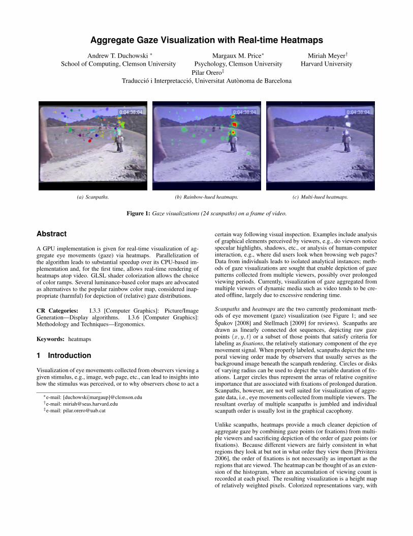
(a) Scanpaths. (b) Rainbow-hued heatmaps. (c) Multi-hued heatmaps.

Figure 1: Gaze visualizations (24 scanpaths) on a frame of video.

Abstract

A GPU implementation is given for real-time visualization of ag-gregate eye movements (gaze) via heatmaps. Parallelization ofthe algorithm leads to substantial speedup over its CPU-based im-plementation and, for the first time, allows real-time rendering ofheatmaps atop video. GLSL shader colorization allows the choiceof color ramps. Several luminance-based color maps are advocatedas alternatives to the popular rainbow color map, considered inap-propriate (harmful) for depiction of (relative) gaze distributions.

CR Categories: I.3.3 [Computer Graphics]: Picture/ImageGeneration—Display algorithms. I.3.6 [Computer Graphics]:Methodology and Techniques—Ergonomics.

Keywords: heatmaps

1 Introduction

Visualization of eye movements collected from observers viewing agiven stimulus, e.g., image, web page, etc., can lead to insights intohow the stimulus was perceived, or to why observers chose to act a

∗e-mail: [duchowski|margaup]@clemson.edu†e-mail: miriah@seas.harvard.edu‡e-mail: pilar.orero@uab.cat

certain way following visual inspection. Examples include analysisof graphical elements perceived by viewers, e.g., do viewers noticespecular highlights, shadows, etc., or analysis of human-computerinteraction, e.g., where did users look when browsing web pages?Data from individuals leads to isolated analytical instances; meth-ods of gaze visualizations are sought that enable depiction of gazepatterns collected from multiple viewers, possibly over prolongedviewing periods. Currently, visualization of gaze aggregated frommultiple viewers of dynamic media such as video tends to be cre-ated offline, largely due to excessive rendering time.

Scanpaths and heatmaps are the two currently predominant meth-ods of eye movement (gaze) visualization (see Figure 1; and seeSpakov [2008] and Stellmach [2009] for reviews). Scanpaths aredrawn as linearly connected dot sequences, depicting raw gazepoints (x, y, t) or a subset of those points that satisfy criteria forlabeling as fixations, the relatively stationary component of the eyemovement signal. When properly labeled, scanpaths depict the tem-poral viewing order made by observers that usually serves as thebackground image beneath the scanpath rendering. Circles or disksof varying radius can be used to depict the variable duration of fix-ations. Larger circles thus represent the areas of relative cognitiveimportance that are associated with fixations of prolonged duration.Scanpaths, however, are not well suited for visualization of aggre-gate data, i.e., eye movements collected from multiple viewers. Theresultant overlay of multiple scanpaths is jumbled and individualscanpath order is usually lost in the graphical cacophony.

Unlike scanpaths, heatmaps provide a much cleaner depiction ofaggregate gaze by combining gaze points (or fixations) from multi-ple viewers and sacrificing depiction of the order of gaze points (orfixations). Because different viewers are fairly consistent in whatregions they look at but not in what order they view them [Privitera2006], the order of fixations is not necessarily as important as theregions that are viewed. The heatmap can be thought of as an exten-sion of the histogram, where an accumulation of viewing count isrecorded at each pixel. The resulting visualization is a height mapof relatively weighted pixels. Colorized representations vary, with

ALU

ALU ALU

ALU

Control

DRAM

Cache

(a) Von Neumann single-core CPU.

DRAM

(b) Many-core GPU.

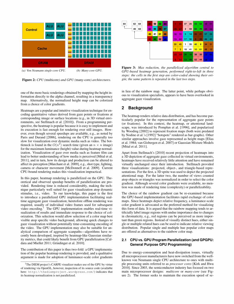
Figure 2: CPU (multicore) and GPU (many-core) architectures.

one of the more basic renderings obtained by mapping the height in-formation directly to the alpha channel, resulting in a transparencymap. Alternatively, the normalized height map can be colorizedfrom a choice of color gradients.

Heatmaps are a popular and intuitive visualization technique for en-coding quantitative values derived from gaze points or fixations atcorresponding image or surface locations (e.g., in 3D virtual envi-ronments, see Stellmach et al. [2010]). From a programming per-spective, the heatmap is popular because it is easy to implement andits execution is fast enough for rendering over still images. How-ever, even though several speedups are available, e.g., as noted byParis and Durand [2006], rendering on the CPU is generally tooslow for visualization over dynamic media such as video. The bot-tleneck is found in the O(n2) search time (given an n × n image)for the maximum luminance (height) value during heatmap normal-ization. Visualization of gaze over media such as feature film canlead to better understanding of how media is perceived [Mital et al.2011], and in turn, how its design and production can be altered toaffect its perception [Marchant et al. 2009], e.g., shot type, lighting,camera or character movement [McDonnell et al. 2009]. CurrentCPU-bound rendering makes this visualization impractical.

In this paper, heatmap rendering is parallelized on the GPU. The-oretical and observed speedup benefits of parallelization are pro-vided. Rendering time is reduced considerably, making the tech-nique particularly well suited for gaze visualization atop dynamicstimulus, i.e., video. To our knowledge, this paper is the firstto introduce a parallelized GPU implementation facilitating real-time aggregate gaze visualization; heretofore offline rendering wasrequired, usually of individual video frames used for subsequentvideo encoding.1 The GPU implementation enables real-time vi-sualization of results and immediate response to the choice of col-orization. This selection would allow selection of a color map bestvisible atop specific video background, allowing quick changes togaze visualization without potentially time-consuming encoding ofthe video. The GPU implementation may also be suitable for an-alytical comparison of aggregate scanpaths—algorithms have re-cently been developed, inspired by heatmap-like Gaussian similar-ity metrics, that could likely benefit from GPU parallelization [Cal-dara and Miellet 2011; Grindinger et al. 2010].

The contribution of this paper is thus two-fold: a GPU implementa-tion of the popular heatmap rendering is provided, and a qualitativeargument is made for adoption of luminance-scale color gradients

1The DIEM project’s CARPE visualizer makes use of the GPU by virtueof rendering via OpenGL, however, inspection of its source code (availablehere: http://thediemproject.wordpress.com/) indicates thatits heatmap normalization is not parallelized.

45

49 52

61

605950

62 56

63

48

5728

64

23

45 41

49 52

61

605950

62 56

63

48

5728

62 64

6349

64

5758

41

59

42

5249

30

43

32

51

23 19

60

54

31

4810

11

12

33

13

21

34

2

3

47

64

44 22

14

16

4

6

24

40

53

25

55

61

38

36

28 46

45 351

37

15

7

5

17

26

18

8

20 9

27 29

56

39

50

62

63

64

23

41

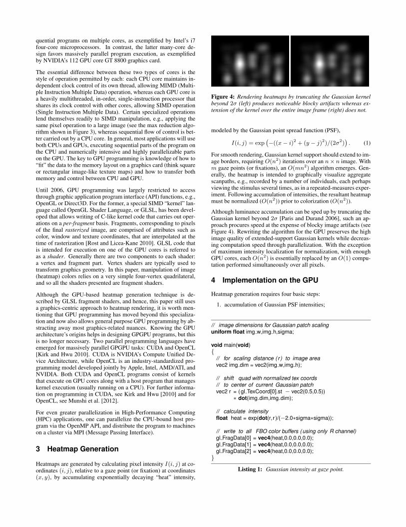
Figure 3: Max reduction, the parallelized algorithm central toGPU-based heatmap generation, performed right-to-left in threesteps: the cells in the first step are color-coded showing their ori-gin; the same pattern is repeated in the last two steps.

in lieu of the rainbow map. The latter point, while perhaps obvi-ous to visualization specialists, appears to have been overlooked inaggregate gaze visualization.

2 Background

The heatmap renders relative data distribution, and has become par-ticularly popular for the representation of aggregate gaze points(or fixations). In this context, the heatmap, or attentional land-scape, was introduced by Pomplun et al. [1996], and popularizedby Wooding [2002] to represent fixation maps (both were predatedby Nodine et al.’s [1992] “hotspots” rendered as bar-graphs). Othersimilar approaches involve gaze represented as height maps [Eliaset al. 1984; van Gisbergen et al. 2007] or Gaussian Mixture Models[Mital et al. 2011].

Apart from Stellmach’s [2010] recent projection of heatmaps intoa 3D depiction of aggregate gaze collected in virtual environments,heatmaps have received relatively little attention and have remainedvirtually unchanged since their introduction. Stellmach providedthree visualizations: projected, object-, and triangle-based repre-sentations. For the first, a 3D sprite was used to depict the projectedattentional map. For the latter two, the number of views countedatop objects or triangles was normalized in order to select the colorgradient. Although several color gradients were available, no men-tion was made of rendering time (complexity) or parallelizability.

The choice of the rainbow gradient can be re-examined becausethe GPU-based implementation facilitates rapid exchange of colormaps. Since heatmaps depict relative frequency, a luminance-scalecolor gradient is advocated as the preferred method for visualizingthis form of data. It is argued that the rainbow mapping tends to ar-tificially label image regions with undue importance due to changesin chromaticity, e.g., red regions can be perceived as more impor-tant than green regions. Instead of visually distinct hues, either sin-gle or multiple related hues can be used to indicate relative viewingdistribution. Popular single and multiple hue popular color mapsare offered as alternatives to the rainbow color map.

2.1 CPU vs. GPU Program Parallelization (and GPGPU:

General Purpose GPU Programming)

Due to energy-consumption and heat-dissipation issues, virtuallyall microprocessor manufacturers have now switched from the well-known von Neumann single CPU architecture to ones with multi-ple processing units referred to as processor cores [Kirk and Hwu2010]. Since 2003, the semiconductor industry has focused on twomain microprocessor designs: multicore or many-core (see Fig-ure 2). The former seeks to maintain the execution speed of se-

quential programs on multiple cores, as exemplified by Intel’s i7four-core microprocessors. In contrast, the latter many-core de-sign favors massively parallel program execution, as exemplifiedby NVIDIA’s 112 GPU core GT 8800 graphics card.

The essential difference between these two types of cores is thestyle of operation permitted by each: each CPU core maintains in-dependent clock control of its own thread, allowing MIMD (Multi-ple Instruction Multiple Data) operation, whereas each GPU core isa heavily multithreaded, in-order, single-instruction processor thatshares its clock control with other cores, allowing SIMD operation(Single Instruction Multiple Data). Certain specialized operationslend themselves readily to SIMD manipulation, e.g., applying thesame pixel operation to a large image (see the max reduction algo-rithm shown in Figure 3), whereas sequential flow of control is bet-ter carried out by a CPU core. In general, most applications will useboth CPUs and GPUs, executing sequential parts of the program onthe CPU and numerically intensive and highly parallelizable partson the GPU. The key to GPU programming is knowledge of how to“fit” the data to the memory layout on a graphics card (think squareor rectangular image-like texture maps) and how to transfer bothmemory and control between CPU and GPU.

Until 2006, GPU programming was largely restricted to accessthrough graphic application program interface (API) functions, e.g.,OpenGL or Direct3D. For the former, a special SIMD “kernel” lan-guage called OpenGL Shader Language, or GLSL, has been devel-oped that allows writing of C-like kernel code that carries out oper-ations on a per-fragment basis. Fragments, corresponding to pixelsof the final rasterized image, are comprised of attributes such ascolor, window and texture coordinates, that are interpolated at thetime of rasterization [Rost and Licea-Kane 2010]. GLSL code thatis intended for execution on one of the GPU cores is referred toas a shader. Generally there are two components to each shader:a vertex and fragment part. Vertex shaders are typically used totransform graphics geometry. In this paper, manipulation of image(heatmap) colors relies on a very simple four-vertex quadrilateral,and so all the shaders presented are fragment shaders.

Although the GPU-based heatmap generation technique is de-scribed by GLSL fragment shaders, and hence, this paper still usesa graphics-centric approach to heatmap rendering, it is worth men-tioning that GPU programming has moved beyond this specializa-tion and now also allows general purpose GPU programming by ab-stracting away most graphics-related nuances. Knowing the GPUarchitecture’s origins helps in designing GPGPU programs, but thisis no longer necessary. Two parallel programming languages haveemerged for massively parallel GPGPU tasks: CUDA and OpenCL[Kirk and Hwu 2010]. CUDA is NVIDIA’s Compute Unified De-vice Architecture, while OpenCL is an industry-standardized pro-gramming model developed jointly by Apple, Intel, AMD/ATI, andNVIDIA. Both CUDA and OpenCL programs consist of kernelsthat execute on GPU cores along with a host program that manageskernel execution (usually running on a CPU). For further informa-tion on programming in CUDA, see Kirk and Hwu [2010] and forOpenCL, see Munshi et al. [2012].

For even greater parallelization in High-Performance Computing(HPC) applications, one can parallelize the CPU-bound host pro-gram via the OpenMP API, and distribute the program to machineson a cluster via MPI (Message Passing Interface).

3 Heatmap Generation

Heatmaps are generated by calculating pixel intensity I(i, j) at co-ordinates (i, j), relative to a gaze point (or fixation) at coordinates(x, y), by accumulating exponentially decaying “heat” intensity,

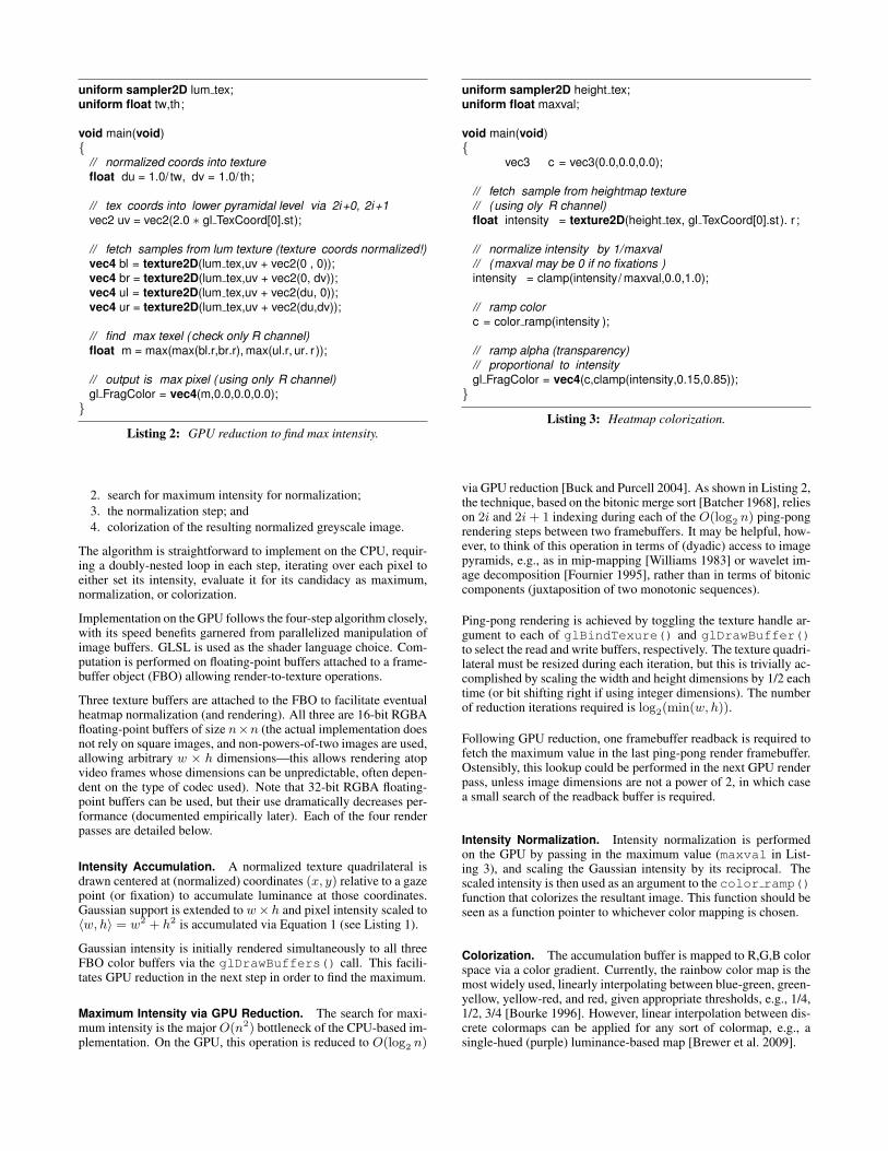
Figure 4: Rendering heatmaps by truncating the Gaussian kernelbeyond 2σ (left) produces noticeable blocky artifacts whereas ex-tension of the kernel over the entire image frame (right) does not.

modeled by the Gaussian point spread function (PSF),

I(i, j) = exp�−((x− i)2 + (y − j)2)/(2σ

2)�

. (1)

For smooth rendering, Gaussian kernel support should extend to im-age borders, requiring O(n2) iterations over an n× n image. Withm gaze points (or fixations), an O(mn

2) algorithm emerges. Gen-erally, the heatmap is intended to graphically visualize aggregatescanpaths, e.g., recorded by a number of individuals, each perhapsviewing the stimulus several times, as in a repeated-measures exper-iment. Following accumulation of intensities, the resultant heatmapmust be normalized (O(n2)) prior to colorization (O(n2)).

Although luminance accumulation can be sped up by truncating theGaussian kernel beyond 2σ [Paris and Durand 2006], such an ap-proach procures speed at the expense of blocky image artifacts (seeFigure 4). Rewriting the algorithm for the GPU preserves the highimage quality of extended-support Gaussian kernels while decreas-ing computation speed through parallelization. With the exceptionof maximum intensity localization for normalization, with enoughGPU cores, each O(n2) is essentially replaced by an O(1) compu-tation performed simultaneously over all pixels.

4 Implementation on the GPU

Heatmap generation requires four basic steps:

1. accumulation of Gaussian PSF intensities;

// image dimensions for Gaussian patch scaling

uniform float img w,img h,sigma;

void main(void){

// for scaling distance ( r ) to image area

vec2 img dim = vec2(img w,img h);

// shift quad with normalized tex coords

// to center of current Gaussian patch

vec2 r = (gl TexCoord[0].st − vec2(0.5,0.5))∗ dot(img dim,img dim);

// calculate intensity

float heat = exp(dot(r,r )/(−2.0∗sigma∗sigma));

// write to all FBO color buffers (using only R channel)

gl FragData[0] = vec4(heat,0.0,0.0,0.0);gl FragData[1] = vec4(heat,0.0,0.0,0.0);gl FragData[2] = vec4(heat,0.0,0.0,0.0);

}

Listing 1: Gaussian intensity at gaze point.

uniform sampler2D lum tex;uniform float tw,th;

void main(void){

// normalized coords into texture

float du = 1.0/ tw, dv = 1.0/ th;

// tex coords into lower pyramidal level via 2i+0, 2i+1

vec2 uv = vec2(2.0 ∗ gl TexCoord[0].st);

// fetch samples from lum texture (texture coords normalized!)

vec4 bl = texture2D(lum tex,uv + vec2(0 , 0));vec4 br = texture2D(lum tex,uv + vec2(0, dv));vec4 ul = texture2D(lum tex,uv + vec2(du, 0));vec4 ur = texture2D(lum tex,uv + vec2(du,dv));

// find max texel (check only R channel)

float m = max(max(bl.r,br.r), max(ul.r, ur. r ));

// output is max pixel (using only R channel)

gl FragColor = vec4(m,0.0,0.0,0.0);}

Listing 2: GPU reduction to find max intensity.

2. search for maximum intensity for normalization;3. the normalization step; and4. colorization of the resulting normalized greyscale image.

The algorithm is straightforward to implement on the CPU, requir-ing a doubly-nested loop in each step, iterating over each pixel toeither set its intensity, evaluate it for its candidacy as maximum,normalization, or colorization.

Implementation on the GPU follows the four-step algorithm closely,with its speed benefits garnered from parallelized manipulation ofimage buffers. GLSL is used as the shader language choice. Com-putation is performed on floating-point buffers attached to a frame-buffer object (FBO) allowing render-to-texture operations.

Three texture buffers are attached to the FBO to facilitate eventualheatmap normalization (and rendering). All three are 16-bit RGBAfloating-point buffers of size n×n (the actual implementation doesnot rely on square images, and non-powers-of-two images are used,allowing arbitrary w × h dimensions—this allows rendering atopvideo frames whose dimensions can be unpredictable, often depen-dent on the type of codec used). Note that 32-bit RGBA floating-point buffers can be used, but their use dramatically decreases per-formance (documented empirically later). Each of the four renderpasses are detailed below.

Intensity Accumulation. A normalized texture quadrilateral isdrawn centered at (normalized) coordinates (x, y) relative to a gazepoint (or fixation) to accumulate luminance at those coordinates.Gaussian support is extended to w× h and pixel intensity scaled to�w, h� = w

2 + h2 is accumulated via Equation 1 (see Listing 1).

Gaussian intensity is initially rendered simultaneously to all threeFBO color buffers via the glDrawBuffers() call. This facili-tates GPU reduction in the next step in order to find the maximum.

Maximum Intensity via GPU Reduction. The search for maxi-mum intensity is the major O(n2) bottleneck of the CPU-based im-plementation. On the GPU, this operation is reduced to O(log2 n)

uniform sampler2D height tex;uniform float maxval;

void main(void){

vec3 c = vec3(0.0,0.0,0.0);

// fetch sample from heightmap texture

// (using oly R channel)

float intensity = texture2D(height tex, gl TexCoord[0].st ). r ;

// normalize intensity by 1/maxval

// (maxval may be 0 if no fixations )

intensity = clamp(intensity/ maxval,0.0,1.0);

// ramp color

c = color ramp(intensity );

// ramp alpha (transparency)

// proportional to intensity

gl FragColor = vec4(c,clamp(intensity,0.15,0.85));}

Listing 3: Heatmap colorization.

via GPU reduction [Buck and Purcell 2004]. As shown in Listing 2,the technique, based on the bitonic merge sort [Batcher 1968], relieson 2i and 2i + 1 indexing during each of the O(log2 n) ping-pongrendering steps between two framebuffers. It may be helpful, how-ever, to think of this operation in terms of (dyadic) access to imagepyramids, e.g., as in mip-mapping [Williams 1983] or wavelet im-age decomposition [Fournier 1995], rather than in terms of bitoniccomponents (juxtaposition of two monotonic sequences).

Ping-pong rendering is achieved by toggling the texture handle ar-gument to each of glBindTexure() and glDrawBuffer()to select the read and write buffers, respectively. The texture quadri-lateral must be resized during each iteration, but this is trivially ac-complished by scaling the width and height dimensions by 1/2 eachtime (or bit shifting right if using integer dimensions). The numberof reduction iterations required is log2(min(w, h)).

Following GPU reduction, one framebuffer readback is required tofetch the maximum value in the last ping-pong render framebuffer.Ostensibly, this lookup could be performed in the next GPU renderpass, unless image dimensions are not a power of 2, in which casea small search of the readback buffer is required.

Intensity Normalization. Intensity normalization is performedon the GPU by passing in the maximum value (maxval in List-ing 3), and scaling the Gaussian intensity by its reciprocal. Thescaled intensity is then used as an argument to the color ramp()function that colorizes the resultant image. This function should beseen as a function pointer to whichever color mapping is chosen.

Colorization. The accumulation buffer is mapped to R,G,B colorspace via a color gradient. Currently, the rainbow color map is themost widely used, linearly interpolating between blue-green, green-yellow, yellow-red, and red, given appropriate thresholds, e.g., 1/4,1/2, 3/4 [Bourke 1996]. However, linear interpolation between dis-crete colormaps can be applied for any sort of colormap, e.g., asingle-hued (purple) luminance-based map [Brewer et al. 2009].

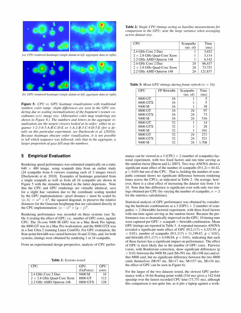
(a) CPU-rendered heatmaps (single datum at left, aggregate data at right).

(b) GPU-rendered heatmaps (single datum at left, aggregate data at right).

Figure 5: CPU vs. GPU heatmap visualizations with traditionalrainbow color ramp: slight differences are seen in the GPU ren-dering due to scaling (normalization) of the fragment’s texture co-ordinates w.r.t. image size. (Alternative color map renderings areshown in Figure 8.) The numbers and letters in the aggregate vi-sualization are the targets viewers looked at in order: either in se-quence 1-2-3-4-5-A-B-C-D-E or 1-A-2-B-3-C-4-D-5-E (for a de-tails on this particular experiment, see Duchowski et al. [2010]).Because heatmaps obscure order visualization, it is not possibleto tell which sequence was followed, only that in the aggregate, alarger proportion of gaze fell atop the numbers.

5 Empirical Evaluation

Rendering speed performance was estimated empirically on a static640 × 480 image, using scanpath data from an earlier study(24 scanpaths from 6 viewers scanning each of 2 images twice)[Duchowski et al. 2010]. Examples of heatmaps generated froma single scanpath as well as from all 24 scanpaths are shown inFigure 5 with the stimulus blended in the latter depictions. Notethat the CPU and GPU renderings are virtually identical, savefor a slight hue variation due to the coordinate scaling neededby the GPU implementation—pixel distance r must be scaled by�w, h� = w

2 + h2, the squared diagonal, to preserve the relative

distances for the Gaussian heightmap that are calculated directly inthe CPU implementation: (x− i)2 + (y − j)2.

Rendering performance was recorded on three systems (see Ta-ble 1) testing the effect of GPU, i.e., number of GPU cores, againstCPU. The 16-core 9400 M GPU was in a Mac Book Pro laptop,the 8800 GT was in a Mac Pro workstation, and the 8800 GTX wasin a Sun Ultra 2 (running Linux CentOS). For GPU evaluation, thefloat-point bitwidth was varied between 16 and 32 bits, and, for bothsystems, timings were obtained by rendering 1 or 24 scanpaths.

From an experimental design perspective, analysis of CPU perfor-

Table 1: Systems tested.

CPU GPU GPU(GeForce) cores

2.4 GHz Core 2 Duo 9400 M 162 × 2.8 GHz Quad-Core Xeon 8800 GT 1122.2 GHz AMD Opteron 148 8800 GTX 128

Table 2: Single CPU timings acting as baseline measurements forcomparison to the GPU; note the large variance when averagingacross dataset size.

CPU Scanpaths Time(no. of) (ms)

2.4 GHz Core 2 Duo 1 3,6522 × 2.8 GHz Quad-Core Xeon 1 3,1142.2 GHz AMD Opteron 148 1 6,1422.4 GHz Core 2 Duo 24 86,4372 × 2.8 GHz Quad-Core Xeon 24 73,7512.2 GHz AMD Opteron 148 24 121,837

Table 3: Mean GPU timings during frame refresh (n = 10).

GPU FP Bitwidth Scanpaths Time(no. of) (ms)

8800 GT 16 1 58800 GTX 16 1 59400 M 16 1 388800 GT 16 24 978800 GTX 16 24 739400 M 16 24 5168800 GT 32 1 148800 GTX 32 1 289400 M 32 1 1018800 GT 32 24 2718800 GTX 32 24 5219400 M 32 24 1,708

mance can be viewed as a 3 (CPU) × 2 (number of scanpaths) fac-torial experiment, with two fixed factors and run time serving asthe random factor [Baron and Li 2007]. Two-way ANOVA shows asignificant main effect of the number of scanpaths (F(1,2) = 44.42,p < 0.05) but not of the CPU. That is, holding the number of scan-paths constant shows no significant difference between renderingtimes across the CPUs, as indicated in Table 2. On average, how-ever, there is a clear effect of increasing the dataset size from 1 to24. Note that this difference is significant even with only two tim-ings obtained per CPU (by varying the number of scanpaths; n = 2for the statistics calculations).

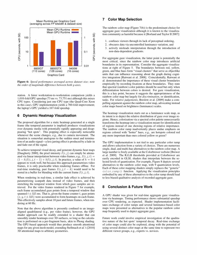
Statistical analysis of GPU performance was obtained by consider-ing the hardware combinations as a 3 (GPU) × 2 (number of scan-paths) × 2 (bitwidth) factorial experiment, with three fixed factorswith run time again serving as the random factor. Because the per-formance was so dramatically improved on the GPU, 10 timing runswere captured per GPU × scanpath × bitwidth combination. MeanGPU timings are reported in Table 3. A repeated measures ANOVArevealed a significant main effect of GPU (F(2,117) = 4,352.95, p< 0.01), number of scanpaths (F(1,117) = 11,199.67, p < 0.01),and bitwidth (F(1,117) = 4,548.04, p < 0.01), indicating that eachof these factors has a significant impact on performance. The effectof GPU is most likely due to the number of GPU cores. Pairwiset-tests, with Bonferroni correction, show significant differences (p< 0.01) between the 9400 M card (M=591 ms, SE=108 ms) and ei-ther 8800 card, but no significant difference between the two 8800cards themselves (M=97 ms, SE=17 ms; M=157 ms, SE=34 ms;the effect of GPU can be seen in Figure 6).

For the larger of the two datasets tested, the slowest GPU perfor-mance with a 16-bit floating-point width (516 ms) gives a 142-foldspeedup over the fastest recorded CPU time (73,751 ms), althoughthis comparison is not quite fair, as it pits a laptop against a work-

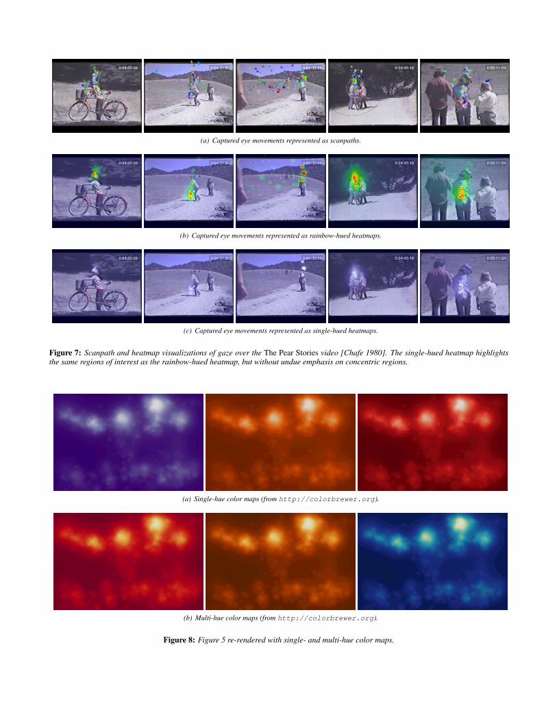
(a) Captured eye movements represented as scanpaths.

(b) Captured eye movements represented as rainbow-hued heatmaps.

(c) Captured eye movements represented as single-hued heatmaps.

Figure 7: Scanpath and heatmap visualizations of gaze over the The Pear Stories video [Chafe 1980]. The single-hued heatmap highlightsthe same regions of interest as the rainbow-hued heatmap, but without undue emphasis on concentric regions.

(a) Single-hue color maps (from http://colorbrewer.org).

(b) Multi-hue color maps (from http://colorbrewer.org).

Figure 8: Figure 5 re-rendered with single- and multi-hue color maps.

1

10

100

8800GT(112 cores)

8800GTX(128 cores)

9400M(16 cores)

0.01

0.1

1

CP

U (s

econ

ds; w

ith S

E)

GP

U (s

econ

ds; w

ith S

E)

Graphics Card

Mean Runtime per Graphics Card(averaging across FP bitwidth & dataset size)

Mean CPU RuntimeMean GPU Runtime

Figure 6: Speed performance averaged across dataset size; notethe order of magnitude difference between both y-axes.

station. A fairer workstation-to-workstation comparison yields a1,010-fold GPU speedup (73 ms vs. 73,751 ms) although this mixesCPU types. Considering just one CPU type (the Quad-Core Xeonin this case), GPU implementation yields a 760-fold improvement;the laptop’s GPU yielded a 167-fold speedup.

6 Dynamic Heatmap Visualization

The proposed algorithm for a static heatmap generated at a singleframe (the temporal parameter is implied) produces visualizationsover dynamic media with potentially rapidly appearing and disap-pearing “hot spots”. This popping effect is especially noticeablewhenever the scene changes, e.g., due to camera movement. Thesituation is somewhat analogous to the sudden onset and termina-tion of an audio signal—a less jarring effect is produced by a fade-inand fade-out of the signal.

To achieve temporal visual decay, and generate dynamic heat maps[Daugherty 2000], the pixel intensity I(i, j) can simply be attenu-ated via linear interpolation between video frames, e.g., I(i, j, t) =(1 − h)I(i, j, t − 1) + hI(i, j, t). In practice, a value of h = 0.4appears to work well, but because this approach parametrizes videoframes, it is only practicable when rendering frames offline. Forreal-time rendering, past frames I(i, j, t − k) would need to bestored in a buffer for blending with the current frame I(i, j, t).

When rendering in real-time, a similar fade effect is achieved byparametrizing scanpath data instead of video frames, and thenstretching the temporal window from which gaze samples are re-trieved. For the video frames rendered in Figure 7 for example,each frame accumulated gaze points from a temporal window thatspanned t± 325 ms. That is, given the frame counter t, gaze points(x, y, t± 325) were accumulated to form heatmaps on each frame.This effectively samples about 10 past and future frames, when ren-dering at 60 Hz.

Note that the above algorithm is presently confined to an image-aligned quadrilateral (e.g., per video frame), however, the GPUshader approach can be readily extended to a shader that cansmoothly render heatmaps over 3D surfaces, so long as the calcula-tion is performed on a per-fragment basis, akin to Phong shading.The GPU-based approach would thus produce smooth attentionalmaps for any given mesh model, extending Stellmach et al.’s [2010]3D attentional maps to arbitrary geometries.

7 Color Map Selection

The rainbow color map (Figure 7(b)) is the predominant choice foraggregate gaze visualization although it is known to the visualiza-tion community as harmful because it [Borland and Taylor II 2007]:

1. confuses viewers through its lack of perceptual ordering,2. obscures data via uncontrolled luminance variation, and3. actively misleads interpretation through the introduction of

non-data-dependent gradients.

For aggregate gaze visualization, the latter point is potentially themost critical, since the rainbow color map introduces artificialboundaries in its representation. Consider the aggregate visualiza-tions at right of Figure 5. The boundaries between red, yellow,green, and blue hues form “visual clusters” that serve as objectlikeunits that can influence reasoning about the graph during cogni-tive integration [Ratwani et al. 2008]. Coincidentally, Ratwani etal. demonstrated the importance of these visual cluster boundariesempirically by recording fixations at these boundaries. They statethat spectral (rainbow) color palettes should be used but only whendifferentiation between colors is desired. For gaze visualization,this is a key point, because it suggests the appropriateness of therainbow color map but largely for discrimination, or identification,tasks. For relative judgements, Breslow et al. [2009] make a com-pelling argument against the rainbow color map, advocating insteadcolor maps based on brightness (luminance) scales.

The heatmap visualization starts out as a luminance scale map, asits intent is to depict the relative distribution of gaze over image re-gions. Hence, colorization via a spectral color palette unnecessarilytransforms the heatmap into a visualization meant for identificationof regions instead of one showing regions of relative importance.The rainbow color ramp inadvertently places undue emphasis onregions colored with “hotter” hues, e.g., are hotspots colored redany more important than ones colored yellow or green?

The GPU implementation is not tied to any particular color rampand allows selection from a variety of choices. There are numeroussingle, dual, and multi-hue alternatives to the rainbow color map. Alarge number is freely available at the Colorbrewer website [Breweret al. 2009]. The R,G,B thresholds provided at Colorbrewer areeasily encoded in GLSL shaders that interpolate between the se-lected levels of quantization. For example, Figure 8 depicts severalalternatives to the rainbow color map, with 9 quantization levels.Each of these color mapping shaders simply replaces the “generic”color ramp() function. Applying the visualization principlesembodied by any of these alternatives to the color ramp should leadto less biased qualitative analysis of recorded aggregate gaze.

8 Conclusion & Future Work

A GPU shader was given for real-time aggregate gaze visualiza-tion via heatmaps. Timing performance shows substantial speedupover CPU rendering, as expected. Shader implementation facili-tates exchange of color ramps and several luminance-based colormaps were presented as alternatives to the popular rainbow colormap frequently used to depict aggregate gaze.

Future work could involve empirical investigation of the qualita-tive nature of the hot spots’ temporal decay. Real-time exchangeof color maps could also be explored, along with the potential ofusing several distinct color maps at the same time to represent twodifferent viewer groups, e.g., experts vs. novices.

References

BARON, J., AND LI, Y., 2007. Notes on the use of R for psychol-ogy experiments and questionnaires. Online Notes, 09 Novem-ber. URL: http://www.psych.upenn.edu/∼baron/rpsych/rpsych.html (last accessed Dec. 2007).

BATCHER, K. E. 1968. Sorting networks and their applications.In Proceedings of the April 30–May 2, 1968, Spring Joint Com-puter Conference, ACM, New York, NY, AFIPS ’68, 307–314.

BORLAND, D., AND TAYLOR II, R. M. 2007. Rainbow ColorMap (Still) Considered Harmful. IEEE Computer Graphics andApplications 27, 2 (March/April), 14–17.

BOURKE, P., 1996. Colour ramping for data visualisation. OnlineTutrial, July. URL: http://local.wasp.uwa.edu.au/∼pbourke/texture colour/colourramp/ (lastaccessed, Dec. 2010).

BRESLOW, L. A., RATWANI, R. M., AND TRAFTON, J. G. 2009.Cognitive Models of the Influence of Color Scale on Data Visu-alization Tasks. Human Factors 51, 3, 321–338.

BREWER, C., HARROWER, M., WOODRUFF, A., AND HEYMAN,D., 2009. Colorbrewer 2.0: Color advice for maps. Online Re-source, Winter. URL: http://colorbrewer2.org (lastaccessed Dec. 2010).

BUCK, I., AND PURCELL, T. 2004. A Toolkit for Computa-tion on GPUs. In GPU Gems: Programming Techniques, Tips,and Tricks for Real-Time Graphics, R. Fernando, Ed. Addison-Wesley, Boston, MA, 621–636.

CALDARA, R., AND MIELLET, S. 2011. iMap: a novel methodfor statistical fixation mapping of eye movement data. BehaviorResearch Methods 43, 3 (April), 864–878.

CHAFE, W. L. 1980. The Deployment of Consciousness in the Pro-duction of a Narrative. In The Pear Stories: Cognitive, Culturaland Linguistic Aspects of Narrative Production, W. L. Chafe, Ed.Ablex Publishing Corporation, Norwood, NJ.

DAUGHERTY, B. 2000. Ocular Vergence Response OverAnaglyphic Stereoscopic Video. Master’s thesis, Clemson Uni-versity, Clemson, SC.

DUCHOWSKI, A. T., DRIVER, J., JOLAOSO, S., RAMEY, B. N.,ROBBINS, A., AND TAN, W. 2010. Scanpath Comparison Re-visited. In Eye Tracking Research & Applications (ETRA), ACM,Austin, TX.

ELIAS, G., SHERWIN, G., AND WISE, J. 1984. Eye movementswhile viewing NTSC format television. Tech. rep., SMPTE Psy-chophysics Subcommittee, March.

FOURNIER, A., Ed. 1995. Course Notes: Wavelets and Their Ap-plications in Computer Graphics, SIGGRAPH 1995, 22nd In-ternational Conference on Computer Graphics and InteractiveTechniques, ACM, New York, NY.

GRINDINGER, T. J., MURALI, V. N., TETREAULT, S.,DUCHOWSKI, A. T., BIRCHFIELD, S. T., AND ORERO, P.2010. Algorithm for Discriminating Aggregate Gaze Points:Comparison with Salient Regions-Of-Interest. In InternationalWorkshop on Gaze Sensing and Interactions, IWGSI/ACCV.

KIRK, D. B., AND HWU, W.-M. W. 2010. Programming Mas-sively Parallel Processors: A Hands-on Approach. MorganKaufmann Publishers, Burlington, MA.

MARCHANT, P., RAYBOULD, D., RENSHAW, T., AND STEVENS,R. 2009. Are You Seeing What I’m Seeing? An Eye-TrackingEvaluation of Dynamic Scenes. Digital Creativity 20, 3, 153–163.

MCDONNELL, R., LARKIN, M., HERNANDEZ, B., RUDOMIN,I., AND O’SULLIVAN, C. 2009. Eye-catching crowds: saliencybased selective variation. In SIGGRAPH ’09: ACM SIGGRAPH2009 papers, ACM, New York, NY, USA, 1–10.

MITAL, P. K., SMITH, T. J., HILL, R. L., AND HENDERSON,J. M. 2011. Clustering of Gaze During Dynamic Scene Viewingis Predicted by Motion. Cognitive Computation 3, 5–24.

MUNSHI, A., GASTER, B. R., MATTSON, T. G., FUNG, J., ANDGINSBURG, D. 2012. OpenCL Programming Guide. PearsonEducation, Inc., Boston, MA.

NODINE, C. F., KUNDEL, H. L., TOTO, L. C., AND KRUPINSKI,E. A. 1992. Recording and analyzing eye-position data using amicrocomputer workstation. Behavior Research Methods 24, 3,475–485.

PARIS, S., AND DURAND, F. 2006. A Fast Approximation of theBilateral Filter using a Signal Processing Approach. Tech. Rep.MIT-CSAIL-TR-2006-073, Massachusetts Inst. of Technology.

POMPLUN, M., RITTER, H., AND VELICHKOVSKY, B. 1996. Dis-ambiguating Complex Visual Information: Towards Communi-cation of Personal Views of a Scene. Perception 25, 8, 931–948.

PRIVITERA, C. M. 2006. The scanpath theory: its definitions andlater developments. In Human Vision and Electronic ImagingXI, SPIE, San Jose, CA, B. E. Rogowitz, T. N. Pappas, and S. J.Daly, Eds.

RATWANI, R. M., TRAFTON, J. G., AND BOEHM-DAVIS, D. A.2008. Thinking Graphically: Connecting Vision and CognitionDuring Graph Comprehension. Journal of Experimental Psy-chology: Applied 14, 1, 36–49.

ROST, R. J., AND LICEA-KANE, B. 2010. OpenGL Shading Lan-guage, 3rd ed. Pearson Education, Inc., Boston, MA.

STELLMACH, S., NACKE, L., AND DACHSELT, R. 2010.3D attentional maps: aggregated gaze visualizations in three-dimensional virtual environments. In Proceedings of the Inter-national Conference on Advanced Visual Interfaces, ACM, NewYork, NY, AVI ’10, 345–348.

STELLMACH, S. 2009. Visual Analysis of Gaze Data in VirtualEnvironments. Master’s thesis, Otto-von-Guericke UniversityMagdeburg, Magdeburg, Germany.

VAN GISBERGEN, M. S., VAN DER MOST, J., AND AELEN,P. 2007. Visual Attention to Online Search Engine Results.Tech. rep., De Vos & Jansen in cooperation with Checkit. URL:http://www.iprospect.nl/wp-content/themes/iprospect/pdf/checkit/eyetracking research.pdf (last accessed Dec. 2011).

SPAKOV, O. 2008. iComponent—Device-Independent Platformfor Analyzing Eye Movement Data and Developing Eye-BasedApplications. PhD thesis, University of Tampere, Finland.

WILLIAMS, L. 1983. Pyramidal Parametrics. Computer Graphics17, 3 (July), 1–11.

WOODING, D. S. 2002. Fixation Maps: Quantifying Eye-Movement Traces. In ETRA ’02: Proceedings of the 2002 Sym-posium on Eye Tracking Research & Applications, ACM, NewYork, NY, 31–36.