af3 advanced forest fire fighting -...

Del. Rev. Date Page

D4.1.2 A 27/01/2016 1 of 37

AF3- Advanced Forest Fire Fighting Grant Agreement no: 607276

AF3

Advanced Forest Fire Fighting

D4.1.2 – Vegetation distribution analysis software and report

PREPARED BY

Edyta Woźniak

SRC PAS

DISSEMINATION LEVEL

PU Public

PP Restricted to other programme participants (including the Commission Services)

RE Restricted to a group specified by the consortium (including the Commission Services)

CO Confidential, only for members of the consortium (including the Commission Services)

Del. Rev. Date Page

D4.1.2 A 27/01/2016 2 of 37


REVISIONS LOG

REV CHANGE REFERENCE DATE CHANGE DESCRIPTION PREPARED

01 2016-01-18 Document created E. Woźniak 02 03

2016-01-22 2016-01-25

Minor changes Additional input

R. Putzar E. Woźniak

04 2016-01-25 Minor changes C. Coveri 05 2016-01-26 Ethical review R. Gowland A 2016-01-27 Final version E. Woźniak

Del. Rev. Date Page

D4.1.2 A 27/01/2016 3 of 37


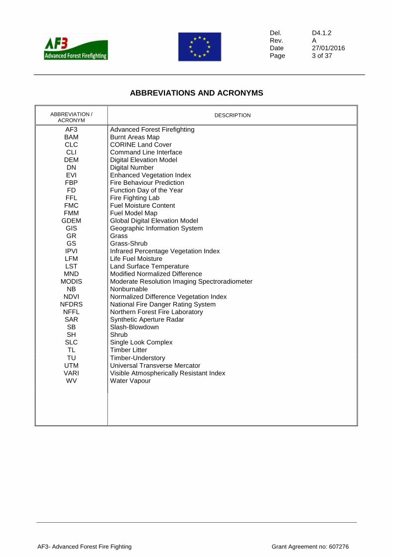
ABBREVIATIONS AND ACRONYMS

ABBREVIATION / ACRONYM

DESCRIPTION

AF3 BAM CLC CLI

DEM DN EVI FBP FD FFL FMC FMM

GDEM GIS GR GS IPVI LFM LST MND

MODIS NB

NDVI NFDRS NFFL

Advanced Forest Firefighting Burnt Areas Map CORINE Land Cover Command Line Interface Digital Elevation Model Digital Number Enhanced Vegetation Index Fire Behaviour Prediction Function Day of the Year Fire Fighting Lab Fuel Moisture Content Fuel Model Map Global Digital Elevation Model Geographic Information System Grass Grass-Shrub Infrared Percentage Vegetation Index Life Fuel Moisture Land Surface Temperature Modified Normalized Difference Moderate Resolution Imaging Spectroradiometer Nonburnable Normalized Difference Vegetation Index National Fire Danger Rating System Northern Forest Fire Laboratory

SAR SB SH SLC

Synthetic Aperture Radar Slash-Blowdown Shrub Single Look Complex

TL Timber Litter

TU UTM VARI WV

Timber-Understory Universal Transverse Mercator Visible Atmospherically Resistant Index Water Vapour

Del. Rev. Date Page

D4.1.2 A 27/01/2016 4 of 37


TABLE OF CONTENTS

TABLE OF FIGURES ........................................................................................................................................ 5

TABLE OF TABLES ......................................................................................................................................... 5

1. SCOPE .......................................................................................................................................... 6

2. REFERENCED DOCUMENTS ..................................................................................................... 6

2.1 CONTRACTUAL DOCUMENTS .................................................................................................. 6

2.2 APPLICABLE DOCUMENTS ....................................................................................................... 6

3. INTRODUCTION ......................................................................................................................... 11

3.1 FUEL MODEL CLASSIFICATIONS ........................................................................................... 11

3.2 REMOTE SENSING APPROCHES FOR MAPPING OF FUEL TYPES .................................... 14

3.3 LIVE FUEL MOISTURE ESTIMATION USING SATELLITE DATA .......................................... 16

4. METHOD ..................................................................................................................................... 17

4.1 FUEL TYPE MAPPING ............................................................................................................... 17

4.1.1 Input data ................................................................................................................................... 17

4.1.2 Data preproccesing ................................................................................................................... 18

4.1.2.1 Landsat 8 .................................................................................................................................... 18

4.1.2.2 Sentinel-1 ................................................................................................................................... 18

4.1.2.2.1 Wishart classification ................................................................................................................... 18

4.1.2.2.2 Multi-temporal analysis ............................................................................................................... 21

4.1.2.3 ASTER Global Digital Elevation Model (ASTER GDEM) ........................................................ 21

4.1.3 Fuel model classification ......................................................................................................... 22

4.1.3.1 Increasing CORINE Land Cover spatial resolution ............................................................... 22

4.1.3.2 Vegetation indices calculation................................................................................................. 23

4.1.3.3 Scatter mechanism statistics in the segments ...................................................................... 24

4.1.3.4 Decision tree development ...................................................................................................... 25

4.2 LIVE FUEL MOISTURE ESTIMATION ...................................................................................... 25

4.2.1 Input data ................................................................................................................................... 25

4.2.2 Method ........................................................................................................................................ 26

5. SOFTWARE DESCRIPTION ...................................................................................................... 28

5.1 FMM PREPROCESSING SOFTWARE ...................................................................................... 28

5.1.1 Software Requirements ............................................................................................................ 28

5.1.2 Pre-configuration ...................................................................................................................... 28

5.1.2.1 Data access................................................................................................................................ 28

5.1.2.2 Area of interest configuration .................................................................................................. 28

5.1.3 Running the application ........................................................................................................... 29

5.1.3.1 Manually ..................................................................................................................................... 29

5.1.3.2 Automatically ............................................................................................................................. 29

5.2 FMM LIBRARY ........................................................................................................................... 30


5.2.1.1 Input Data ................................................................................................................................... 30

5.2.1.2 Opening Action Library in eCognition .................................................................................... 30

Del. Rev. Date Page

D4.1.2 A 27/01/2016 5 of 37


5.2.1.3 Description of Fuel Model Mapping action ............................................................................. 32

5.3 LFM SOFTWARE ....................................................................................................................... 33


5.3.2 Pre-configuration ...................................................................................................................... 34

5.3.2.1 Data access................................................................................................................................ 34

5.3.2.2 Area of interest configuration .................................................................................................. 34

5.3.3 Running the application ........................................................................................................... 35

5.3.3.1 Manually ..................................................................................................................................... 35

5.3.3.2 Automatically ............................................................................................................................. 35

6. CONCLUSIONS .......................................................................................................................... 36

TABLE OF FIGURES

Figure 1. Two-dimensional H/α plane .............................................................................................................. 19 Figure 2. H/alpha plane classification: a) March, b) May, c) July, d) September, e) November ..................... 20 Figure 3. Scattering mechanism stability ......................................................................................................... 21 Figure 4. Slope (a) and aspect (b) maps ......................................................................................................... 21 Figure 5. Hierarchical Landsat image segmentations: a) CLC level; b) II detailed level ................................. 22 Figure 6. Basic statistics: a) mean, b) median, c) majority, d) range and e) variety, calculated for segments based on scatter mechanism image from March. ........................................................................................... 24 Figure 7. Decision tree for the detailed Fuel Model Mapping (example: shrubs) ............................................ 25 Figure 8 Configure Analysis ............................................................................................................................ 30 Figure 9 Open Action Library ........................................................................................................................... 31 Figure 10 Action Library folder ........................................................................................................................ 31 Figure 11 Add Actions ..................................................................................................................................... 32 Figure 12 Raster layers group ......................................................................................................................... 32 Figure 13 Vector layers group ......................................................................................................................... 33 Figure 14 Processing group............................................................................................................................. 33 Figure 15 Description ....................................................................................................................................... 33

TABLE OF TABLES

Table 1. NFDRS fuel classification system [Cohen & Deeming, 1982] ........................................................... 11 Table 2. NFFL fuel classification system [Albini, 1976] ................................................................................... 12 Table 3. Fuel model parameters [Scott & Burgan 2005] ................................................................................. 13 Table 4. FBP system fuel types [Forestry Canada, 1992] ............................................................................... 14 Table 5. Prometheus fuel types [Arroyo et al. 2006] ....................................................................................... 14

Del. Rev. Date Page

D4.1.2 A 27/01/2016 6 of 37


1. SCOPE This report summarizes the findings of task 4.1.2: ‘Distribution analysis of vegetation’ under work package 4.1 of the EU FP7 project AF3 »Advanced Forest Fire Fighting«, grant agreement no. 607276. The aim of the ask 4.1.2 was to determines the distribution of fuel models using high resolution satellite images and estimate a fuel moisture on the base of low resolution MODIS data.

2. REFERENCED DOCUMENTS

2.1 CONTRACTUAL DOCUMENTS

[DoW] Description of Work : Annex 1 to Grant agreement for EU FP7 project AF3 Advanced Forest Fire Fighting. – Grant agreement no. 607276

2.2 APPLICABLE DOCUMENTS

[Albini, 1976] Albini, F.A., 1976. Estimating wildfire behavior and effects. Rep. No. GTR INT-30. USDA, Forest Service, Intermountain Forest and Range Experiment Station, Ogden, UT.

[Alonso et al., 1996] Alonso, M., Camarasa, A., Chuvieco, E., Cocero, D., Kyun, I., Martı´n, M. P., & Salas, F. J. (1996). Estimating temporal dynamics of fuel moisture content of Mediterranean species from NOAA–AVHRR data. EARSEL Advances in Remote Sensing, 4(4), 9 – 24.

[Andersen et al., 2005] Andersen, H.-E., McGaughey, R.J., Reutebuch, S.E., 2005. Estimating forest canopy fuel parameters using LIDAR data. Remote Sensing of Environment 94, 441–449.

[Arroyo et al. 2006] Arroyo, L.A., Healey, S.P., Cohen, W.B., Cocero, D., 2006. Using object-oriented classification and high-resolution imagery to map fuel types in a Mediterranean region. Journal of Geophysical Research 111, G04S04 doi:10.1029/2005JG000120

[Carlson & Burgan, 2003] Carlson, J. D., & Burgan, R. E. (2003). Review of users’ needs in operational fire danger estimation: The Oklahoma example. International Journal of Remote Sensing, 24(8), 1601– 1620.

[Ceccato et al., 2003] Ceccato, P., Leblon, B., Chuvieco, E., Flasse, S., & Carlson, J. D. (2003). Estimation of live fuel moisture content. In E. Chuvieco (Ed.), Wildland fire danger estimation and mapping. The role of remote sensing data (pp. 63–90). Singapore: World Scientific Publishing.

[Chladil & Nunez, 1995] Chladil, M. A., & Nunez, M. (1995). Assessing grassland moisture and biomass in Tasmania. The application of remote sensing and empirical models for a cloudy environment. International Journal of Wildland Fire, 5, 165– 171.

[Chuvieco & Congalton, 1989] Chuvieco, E., Congalton, R.G., 1989. Application of remote sensing and geographic information systems to forest fire hazard mapping. Remote Sensing of Envir- onment 29, 147–159.

[Chuvieco et al. 1999] Chuvieco, E., Carvacho, L., Rodrıiguez-Silva, F., 1999. Integrated fire risk mapping. In: Chuvieco, E. (Ed.), Remote Sensing of Large Wildfires. Springer, Berlin, pp. 61–84.

Del. Rev. Date Page

D4.1.2 A 27/01/2016 7 of 37


[Chuvieco et al. 1999] Chuvieco, E., Deshayes, M., Stach, N., Cocero, D., & Rian˜o, D. (1999). Short-term fire risk: Foliage moisture content estimation from satellite data. In E. Chuvieco (Ed.), Remote sensing of large wildfires in the European Mediterranean Basin ( pp. 17– 38). Berlin: Springer-Verlag.

[Chuvieco et al., 2004] Chuvieco, E., Cocero, D., Rian˜ o, D., Martin, P., Martı´nez-Vega, J., Riva, J.d.l., Pe´ rez, F., 2004. Combining NDVI and surface temperature for the estimation of live fuel moisture content in forest fire danger rating. Remote Sensing of Environment 92, 322–331.

[Cloude & Pottier, 1997] Cloude, S.R., Pottier, E. 1997. An entropy based classification scheme for land application of polarimetric SAR. IEEE Transactions on Geoscience and Remote Sensing, 35 (1), p. 68-78.

[Cohen & Deeming, 1982] Cohen, J.D., Deeming, J.E., 1982. The National Fire Danger Rating System: basic equations. Rep. No. PSW-82. Pacific Southwest Forest and Range Experiment Station, Berkeley, CA.

[Crippen, 1990] Crippen, R. 1990. Calculating the Vegetation Index Faster. Remote Sensing of Environment 34, pp. 71-73.

[Deeming et al. 1972] Deeming, J.E., Lancaster, J.W., Fosberg, M.A., Furman, R.W., Schroeder, M.J., 1972. The National Fire-Danger Rating System. Rep. No. RM-84. USDA Forest Service, Ogden, UT.

[Forestry Canada, 1992] Forestry Canada, 1992. Development and structure of the Canadian Forest Fire Behavior Prediction System. Rep. No. ST-X-3. Forestry Canada, Ottawa.

[Garestier et al., 2008] Garestier, F., Dubois-Fernandez, P.C., Papathanassiou, K.P., 2008. Pine forest height inversion using single-pass X-band PolInSAR data. IEEE Transactions on Geoscience and Remote Sensing 46, 59–68.

[Gitelson et al., 2002] Gitelson, A., Stark, R., Grits, U., Rundquist, D., Kaufman, Y., Derry, D. 2002. Vegetation and Soil Lines in Visible Spectral Space: A Concept and Technique for Remote Estimation of Vegetation Fraction. International Journal of Remote Sensing 23, pp. 2537−2562

[Gitelson et al., 2006] Gitelson, A., and M. Merzlyak. 1998. Remote Sensing of Chlorophyll Concentration in Higher Plant Leaves. Advances in Space Research 22, pp. 689-692

[Harrell et al. 1995] Harrell, P., Bourgeau-Chavez, L.L., Kasischke, E.S., French, N.H.F., Christensen, N.L.J., 1995. Sensitivity of ERS-1 and JERS-1 radar data to biomass and stand structure in Alaskan boreal forest. Remote Sensing of Environment 54, 247–260.

[Huete et al. 2002] Huete, A., Didan, K., Miura, T., Rodriguez, E.P., Gao, X., Ferreira, L.G. 2002. Overview of the radiometric and biophysical performance of the MODIS vegetation indices. Remote Sensing of Environment 83, pp. 195-213

Del. Rev. Date Page

D4.1.2 A 27/01/2016 8 of 37


[James et al. 2007] James, P.M.A., Fortin, M.-J., Fall, A., Kneeshaw, D., Messier, C., 2007. The effects of spatial legacies following shifting management practices and fire on boreal forest age structure. Ecosystems 10, 1261–1277 doi:10.1007/s10021-007- 9095-y.

[Keane et al. 2001] Keane, R.E., Burgan, R.E., van Wagtendonk, J., 2001. Mapping wildland fuel for fire management across multiple scales: Integrating remote sensing, GIS, and biophysical modeling. International Journal of Wildland Fire 10, 301–319.

[Keramitsoglou et al. 2008] Keramitsoglou, I., Kontoes, C., Sykioti, O., Sifakis, N., Xofis, P., 2008. Reliable, accurate and timely forest mapping for wildfire management using ASTER and Hyperion satellite imagery. Forest Ecology and Management 255, 3556–3562.

[Kourtz, 1977] Kourtz, P.H., 1977. An application of Landsat digital technology to forest fire fuel type mapping. In: 11th International Symposium on Remote Sensing of Envir- onment, Ann Arbor, pp. 1111–1115.

[Lasaponara & Lanorte, 2007a] Lasaponara, R., Lanorte, A., 2007a. On the capability of satellite VHR QuickBird data for fuel type characterization in fragmented landscape. Ecological Modelling 204, 79–84.

[Lasaponara & Lanorte, 2007b] Lasaponara, R., Lanorte, A., 2007b. Remotely sensed characterization of forest fuel types by using satellite ASTER data. International Journal of Applied Earth Observation and Geoinformation 9, 225–234.

[Leblon, 2001] Leblon, B. (2001). Forest wildfire hazard monitoring using remote sensing: A review. Remote Sensing Reviews, 20(1), 1 –57.

[Lee, 1941] Lee, H.C., 1941. Aerial photography: a method for fuel type mapping. Journal of Forestry 39, 531–533.

[Lee at al. 1999] Lee, J.S., Grunes, M.R., Ainsworth, T.L. Du. L., Cloude, S.R. 1999. Unsupervised classification using polarimetric decomposition and the complex Wishart Classifier. IEEE Transactions on Geoscience and Remote Sensing, 37 (5), p. 2249-2258.

[Mallinis et al. 2014] Mallinis, G., Galidaki, G., Gitas, I. 2014. A Comparative Analysis of EO-1 Hyperion, Quickbird and Landsat TM Imagery for Fuel Type Mapping of a Typical Mediterranean Landscape. Remote Sensing 6, p. 1984-1704.

[McArtur 1966] McArthur, A.G., 1966. Weather and grassland fire behaviour. Australian Forestry and Timber Bureau Leaflet, no. 100.

[McArtur 1967] McArthur, A.G., 1967. Fire behaviour in eucalypt forests. Australian Forestry and Timber Bureau Leaflet, no. 107.

[Mutlu et al., 2008] Mutlu, M., Popescu, S.C., Stripling, C., Spencer, T., 2008. Mapping surface fuel models using lidar and multispectral data fusion for fire behavior. Remote Sensing of Environment 112, 274–285.

[Paltridge & Barber, 1988] Paltridge, G., Barber, J. 1988. Mornitoring grassland dryness and fire potential in Australia with noaa/avhrr data. Rem. Sens. of Environ.

Del. Rev. Date Page

D4.1.2 A 27/01/2016 9 of 37


[Prosper-Laget et al., 1995] Prosper-Laget, V., Dougue´droit, A., & Guinot, J. P. (1995). Mapping the risk of forest fire occurrence using NOAA satellite information. EARSEL Advances in Remote Sensing, 4(3), 30– 38.

[Riano et al., 2002] Riano, D., Chuvieco, E., Salas, F.J., Palacios-Orueta, A., Bastarrica, A., 2002. Generation of fuel type maps from Landsat TM images and ancillary data in Mediterranean ecosystems. Canadian Journal of Forest Research 32, 1301–1315.

[Riano et al., 2003] Riano, D., Meier, E., Allgower, B., Chuvieco, E., Ustin, S.L., 2003. Modeling airborne laser scanning data for the spatial generation of critical forest parameters in fire behavior modeling. Remote Sensing of Environment 86, 177–186.

[Riano et al., 2004] Riano, D., Chuvieco, E., Condes, S., Gonzalez-Matesanz, J., Ustin, S.L., 2004. Genera- tion of crown bulk density for Pinus sylvestris L. from lidar. Remote Sensing of Environment 92, 345–352.

[Roberts et al. 1998] Roberts, D.A., Gardner, M., Church, R., Ustin, S., Scheer, G., Green, R.O., 1998. Mapping chaparral in the Santa Monica Mountains using multiple endmember spectral mixture models. Remote Sensing of Environment 65, 267–279.

[Rothermel, 1972] Rothermel, R.C. 1972. A mathematical model for predicting fire spread in wildland fuels. USDA Forest Service Research Paper INT-115.

[Rouse et al. 1974] Rouse J.W., Haas R.H., Schell J.A. & Deering D.W. 1974. Monitoring vegetation systems in the Great Plains with ERTS. In: Fraden S.C., Marcanti E.P. & Becker M.A. (eds.), Third ERTS-1 Symposium, 10–14 Dec. 1973, NASA SP-351, Washington D.C. NASA, pp. 309–317.

[Saatchi et al., 2007] Saatchi, S., Halligan, K., Despain, D.G., Crabtree, R.L., 2007. Estimation of forest fuel load from radar remote sensing. IEEE Transactions on Geoscience and Remote Sensing 45, 1726–1740.

[Scott & Burgan 2005] Scott, J.H.; Burgan, R.E. 2005. Standard fire behavior fuel models: a comprehensive set for use with Rothermel’s surface fire spread model. Gen. Tech. Rep. RMRS-GTR-153. Fort Collins, CO: U.S. Department of Agriculture, Forest Service, Rocky Mountain Research Station. 72 p.

[Show & Kotok, 1929] Show, S.B., Kotok, E.I., 1929. Cover type and fire control in the national forests of northern California. Rep. No. 1495. USDA, Forest Services, Washington, DC.

[Skowronski et al., 2007] Skowronski, N., Clark, K., Nelson, R., Hom, J., Patterson, M., 2007. Remotely sensed measurements of forest structure and fuel loads in the Pinelands of New Jersey. Remote Sensing of Environment 108, 123–129.

[Sobrino et al., 2003] Sobrino, J.A., Kharraz, J.E., Li, Z.L. (2003). Surface temperature and water vapour retrieval from MODIS data. International Journal Of Remote Sensing, 24(24), 5161-5182.

Del. Rev. Date Page

D4.1.2 A 27/01/2016 10 of 37


[Varga & Asner, 2008] Varga, T.A., Asner, G.P., 2008. Hyperspectral and lidar remote sensing of fire fuels in Hawaii Volcanoes National Park. Ecological Applications 18, 613–623.

[Vidal et al., 1994] Vidal, A., Pinglo, F., Durand, H., Devaux-Ros, C., & Maillet, A. (1994). Evaluation of a temporal fire risk index in Mediterranean forest from NOAA thermal IR. Remote Sensing of Environment, 49, 296– 303.

[Zarco-Tejada et al., 2003] Zarco-Tejada, P. J., Rueda, C. A., & Ustin, S. L. (2003). Water content estimation in vegetation with MODIS reflectance data and model inversion methods. Remote Sensing of Environment, 85, 109– 124.

Del. Rev. Date Page

D4.1.2 A 27/01/2016 11 of 37


3. INTRODUCTION

3.1 FUEL MODEL CLASSIFICATIONS

Fuel models map presents groups of fuel which are characterized by specific live and dead fuel load, fuel bed depth and determine a fire behaviour at the flaming front, postfrontal combustion, fuel consumption, smoke production, and crown fire behaviour. Several fire models use different fuel classifications: starting from very simple divisions of fuels: grasslands and forest [McArtur 1966, 1967] ending with complex fuel division system which distinguishes 48 classes [Scott & Burgan 2005].

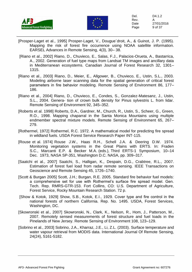
In the United States, the National Fire Danger Rating System (NFDRS) was created in the 70’s [Deeming et al. 1972]. The NFDRS fuel models were adjusted to everyday and seasonal trends in fire danger. Originally the system distinguished 9 fire fuel types which finally were extended to 20 classes [Cohen & Deeming, 1982] (Table 1).

Table 1. NFDRS fuel classification system [Cohen & Deeming, 1982]

Fuel type Fuel model Fuel parameters Fuel loadings (t/acre)1

1 h2 10 h3 100 h4

1000 h5

Wood6

Herb7

Fuel depth (ft)8

Moisture

of extinction

dead fuels (%)9

Western grasses (annual)

Western grasses (periannial)

Sawgrass

Pine-grass savanna

Southern rough

Sagebrush-grass

California chaparral

Intermediate brush

Hardwood litter (winter)

Southern pine plantation

Hardwood litter (summer)

Western pines

Heavy slash

Intermediate slash

Light slash

High pocosin

Tundra

Short-needle conifer (normal dead)

Short-needle conifer (heavy dead)

Alaskan black spruce

A

L

N

C

D

T

B

F

E

P

R

U

I

J

K

O

S

H

G

Q

0.2

0.25

1.5

0.4

2.0

1.0

3.5

2.5

1.5

1.0

0.5

1.5

12.0

7.0

2.5

2.0

0.5

1.5

2.5

2.0

1.5

1.0

1.0

0.5

4.0

2.0

0.5

1.0

0.5

1.5

12.0

7.0

2.5

3.0

0.5

1.0

2.0

2.5

0.5

1.5

0.25

0.5

0.5

1.0

10.0

6.0

2.0

3.0

0.5

2.0

5.0

2.0

12.0

5.5

2.5

2.0

0.5

2.0

12.0

1.0

2.0

0.5

3.0

2.5

11.5

9.0

0.5

0.5

0.5

0.5

7.0

0.5

0.5

0.5

4.0

0.3

0.5

0.8

0.75

0.5

0.5

0.5

0.5

0.5

0.5

0.5

0.5

0.5

0.8

1.0

3.0

0.75

2.0

1.25

4.5

4.5

0.4

0.4

0.25

0.5

2.0

1.3

0.6

4.0

0.4

0.3

1.0

3.0

15

15

25

10

30

15

15

15

25

30

25

20

25

25

25

30

25

20

25

25

1 For each fuel model, the top value is surface-area-to-volume ratio (ft-1), and the bottom value is fuel loading (tons/acre). 21-hour timelag dead fuel moisture class. 310-hour timelag dead fuel moisture class. 4100-hour timelag dead fuel moisture class. 51000-hour timelag dead fuel moisture class. 6Live fine woody fuel class. 7Live fine herbaceous fuel class. 8Effective fuel bed depth. 9Assigned dead fuel moisture of extinction.

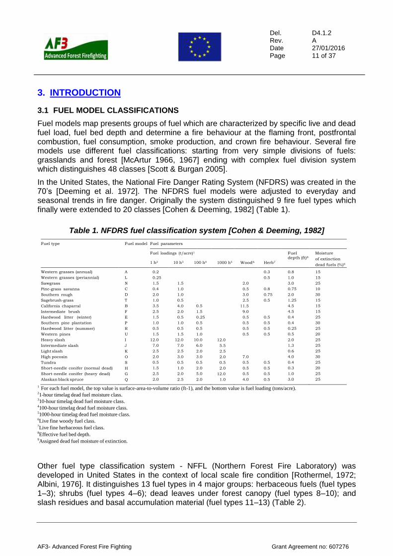
Other fuel type classification system - NFFL (Northern Forest Fire Laboratory) was developed in United States in the context of local scale fire condition [Rothermel, 1972; Albini, 1976]. It distinguishes 13 fuel types in 4 major groups: herbaceous fuels (fuel types 1–3); shrubs (fuel types 4–6); dead leaves under forest canopy (fuel types 8–10); and slash residues and basal accumulation material (fuel types 11–13) (Table 2).

Del. Rev. Date Page

D4.1.2 A 27/01/2016 12 of 37


Table 2. NFFL fuel classification system [Albini, 1976]

Fuel type Fuel model Fuel parameters

Fuel loadings (t/ha)1

1 h2 10 h3

100 h4

Life5

Fuel depth (ft)6 Moisture of

extinction dead

fuels (%)7

Grass and grass-dominated

1

0.74

1.00

0.50

0.50

1.0

12 Short grass (30 cm)

Timber 2 2.00 1.0 15

Tall grass (76 cm) 3 3.01 2.5 25

Chaparral and shrub fields 5.01 Chaparral (18 cm) 4 5.01 4.01 2.00 2.00 6.0 20

Brush (61 cm) 5 1.00 0.50 2.0 20

Dormant brush, hardwood

slash

6 1.50 2.50 2.00 0.37 2.5 25

Southern rough 7 1.13 1.87 1.50 2.5 40

Timber litter Closed timber litter 8 1.50 1.00 2.50 0.2 30

Hardwood litter 9 2.92 0.41 0.15 0.2 25

Timber (litter and understory) 10 3.01 2.00 5.01 2.00 1.0 25

Slash Light logging slash 11 1.50 4.51 5.51 1.0 15

Medium logging slash 12 4.01 14.03 16.53 2.3 20

Heavy jogging slash 13 7.01 23.04 28.05 3.0 25

1 For each fuel model, the top value is surface-area-to-volume ratio (ft-1), and the bottom value is fuel loading (tons/hectares). 21-hour timelag dead fuel moisture class. 310-hour timelag dead fuel moisture class. 4100-hour timelag dead fuel moisture class. 5 Life fuel class. 6Effective fuel bed depth. 7Assigned dead fuel moisture of extinction.

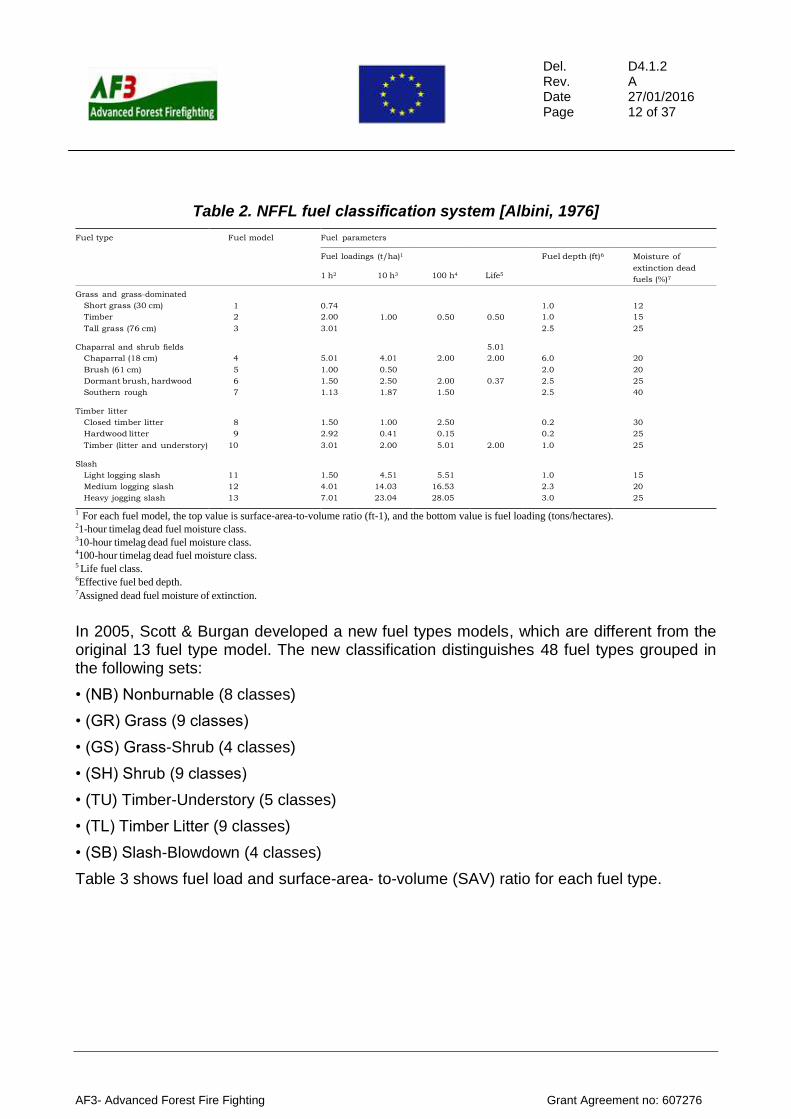
In 2005, Scott & Burgan developed a new fuel types models, which are different from the original 13 fuel type model. The new classification distinguishes 48 fuel types grouped in the following sets:

• (NB) Nonburnable (8 classes)

• (GR) Grass (9 classes)

• (GS) Grass-Shrub (4 classes)

• (SH) Shrub (9 classes)

• (TU) Timber-Understory (5 classes)

• (TL) Timber Litter (9 classes)

• (SB) Slash-Blowdown (4 classes)

Table 3 shows fuel load and surface-area- to-volume (SAV) ratio for each fuel type.

Del. Rev. Date Page

D4.1.2 A 27/01/2016 13 of 37


Table 3. Fuel model parameters [Scott & Burgan 2005]

Fuel

Fuel load (t/ac)

Fuel

SAV ratio (1/ft)b

Fuel

bed

Dead fuel

extinction

model Live Live model Dead Live Live depth moisture

code 1-hr 10-hr 100-hr herb woody typea 1-hr herb woody (ft) (percent)

GR1 0.10 0.00 0.00 0.30 0.00 dynamic 2200 2000 9999 0.4 15

GR2 0.10 0.00 0.00 1.00 0.00 dynamic 2000 1800 9999 1.0 15

GR3 0.10 0.40 0.00 1.50 0.00 dynamic 1500 1300 9999 2.0 30

GR4 0.25 0.00 0.00 1.90 0.00 dynamic 2000 1800 9999 2.0 15

GR5 0.40 0.00 0.00 2.50 0.00 dynamic 1800 1600 9999 1.5 40

GR6 0.10 0.00 0.00 3.40 0.00 dynamic 2200 2000 9999 1.5 40

GR7 1.00 0.00 0.00 5.40 0.00 dynamic 2000 1800 9999 3.0 15

GR8 0.50 1.00 0.00 7.30 0.00 dynamic 1500 1300 9999 4.0 30

GR9 1.00 1.00 0.00 9.00 0.00 dynamic 1800 1600 9999 5.0 40

GS1 0.20 0.00 0.00 0.50 0.65 dynamic 2000 1800 1800 0.9 15

GS2 0.50 0.50 0.00 0.60 1.00 dynamic 2000 1800 1800 1.5 15

GS3 0.30 0.25 0.00 1.45 1.25 dynamic 1800 1600 1600 1.8 40

GS4 1.90 0.30 0.10 3.40 7.10 dynamic 1800 1600 1600 2.1 40

SH1 0.25 0.25 0.00 0.15 1.30 dynamic 2000 1800 1600 1.0 15

SH2 1.35 2.40 0.75 0.00 3.85 N/A 2000 9999 1600 1.0 15

SH3 0.45 3.00 0.00 0.00 6.20 N/A 1600 9999 1400 2.4 40

SH4 0.85 1.15 0.20 0.00 2.55 N/A 2000 1800 1600 3.0 30

SH5 3.60 2.10 0.00 0.00 2.90 N/A 750 9999 1600 6.0 15

SH6 2.90 1.45 0.00 0.00 1.40 N/A 750 9999 1600 2.0 30

SH7 3.50 5.30 2.20 0.00 3.40 N/A 750 9999 1600 6.0 15

SH8 2.05 3.40 0.85 0.00 4.35 N/A 750 9999 1600 3.0 40

SH9 4.50 2.45 0.00 1.55 7.00 dynamic 750 1800 1500 4.4 40

TU1 0.20 0.90 1.50 0.20 0.90 dynamic 2000 1800 1600 0.6 20

TU2 0.95 1.80 1.25 0.00 0.20 N/A 2000 9999 1600 1.0 30

TU3 1.10 0.15 0.25 0.65 1.10 dynamic 1800 1600 1400 1.3 30

TU4 4.50 0.00 0.00 0.00 2.00 N/A 2300 9999 2000 0.5 12

TU5 4.00 4.00 3.00 0.00 3.00 N/A 1500 9999 750 1.0 25

TL1 1.00 2.20 3.60 0.00 0.00 N/A 2000 9999 9999 0.2 30

TL2 1.40 2.30 2.20 0.00 0.00 N/A 2000 9999 9999 0.2 25

TL3 0.50 2.20 2.80 0.00 0.00 N/A 2000 9999 9999 0.3 20

TL4 0.50 1.50 4.20 0.00 0.00 N/A 2000 9999 9999 0.4 25

TL5 1.15 2.50 4.40 0.00 0.00 N/A 2000 9999 1600 0.6 25

TL6 2.40 1.20 1.20 0.00 0.00 N/A 2000 9999 9999 0.3 25

TL7 0.30 1.40 8.10 0.00 0.00 N/A 2000 9999 9999 0.4 25

TL8 5.80 1.40 1.10 0.00 0.00 N/A 1800 9999 9999 0.3 35

TL9 6.65 3.30 4.15 0.00 0.00 N/A 1800 9999 1600 0.6 35

SB1 1.50 3.00 11.00 0.00 0.00 N/A 2000 9999 9999 1.0 25

SB2 4.50 4.25 4.00 0.00 0.00 N/A 2000 9999 9999 1.0 25

SB3 5.50 2.75 3.00 0.00 0.00 N/A 2000 9999 9999 1.2 25

SB4 5.25 3.50 5.25 0.00 0.00 N/A 2000 9999 9999 2.7 25

a Fuel model type does not apply to fuel models without live herbaceous load. b The value 9999 was assigned in cases where there is no load in a particular fuel class or category c The same heat content value was applied to both live and dead fuel categories.

Del. Rev. Date Page

D4.1.2 A 27/01/2016 14 of 37


Canadian Fire Behaviour Prediction (FBP) [Forestry Canada, 1992] organizes fire fuels in 16 types, which are grouped into 5 main classes: coniferous, deciduous, mixed wood, slash and open. Fuel types are described qualitatively (Table 4).

Table 4. FBP system fuel types [Forestry Canada, 1992]

Group Identifier Fuel type description

Coniferous C - 1

C - 2

C - 3

C - 4

C - 5

C - 6

C - 7

Spruce-lichen woodland

Boreal spruce

Mature jack or lodgepole pine

Immature jack or lodgepole pine

Red and white pine

Conifer plantation

Ponderosa pine–Douglas-fir

Deciduous D - 1 Leafless aspen

Mixedwood M - 1

M - 2

M - 3

M - 4

Boreal mixedwood—leafless

Boreal mixedwood—green

Dead balsam fir mixedwood—leafless

Dead balsam fir mixedwood—green

Slash S - 1

S - 2

S - 3

Jack or lodgepole pine slash

White spruce-balsam slash

Coastal cedar–hemlock–Douglas-fir slash

Open O - 1 Grass

Prometheus is an European fuel classification system [Arroyo et al. 2006] developed on the base of NFFL. Comparing to the NFFL system the Prometheus is more simplified and adapted to Mediterranean conditions. This system divides fuels into 7 classes (Table 5).

Table 5. Prometheus fuel types [Arroyo et al. 2006]

Fuel type Grass Bushes Trees (> 4m)

F1 > 60%

F2 > 60 % < 50 % Bush mean height 0.6 m F3 > 60 % < 50 % Bush mean height 2 m

F4 > 60 % < 50 % Bush mean height 4 m

F5 < 30 % > 50% F6 > 30 % > 50% Mean distance between bushes and trees: > 0.5 m

F7 > 30 % > 50% Mean distance between bushes and trees: 0 m

Taking into account the requirements of Fire Fighting Lab (FFL) the NFFL fuel type classification system was selected, which is designed for the use at the local scale.

3.2 REMOTE SENSING APPROCHES FOR MAPPING OF FUEL TYPES

Traditionally the fuel types were mapped collecting data in the terrain during the field surveys. Because this approach is very time and resources consuming and could not be applied for large areas [Show & Kotok, 1929], in the 1940’s the idea of using aerial photography to map fuel types gained a huge interest. Although from the beginning some limitation of photo interpretation were pointed out [Lee, 1941] this technique is still considered one of the most suitable method for mapping fuel types [James et al. 2007].

Del. Rev. Date Page

D4.1.2 A 27/01/2016 15 of 37


The modern remote sensing has a large spectrum of passive and active sensors which could be used in fuel type mapping. The optic multispectral and hyperspectral images constitute the major group. The main limitation of these data is their incapacity to penetrate the canopy [Keane et al. 2001] so it is impossible to detect the internal vegetation layers or fuel structure. Moreover, the reflectance describes rather a chemistry of the processes which occur in the plant than the plant shape or height so direct mapping of fuel type is impossible and often requires an additional data.

The very high resolution multispectral data, such as: IKONOS, QuickBird seem to be the most alike to aerial photography because their spatial resolution is around 1 m. So they are considered as a potentially useful in fuel type mapping. The QuickBird images were used to classify fuel types according to the Prometheus classification [Arroyo et al., 2006]. The 7 fuel types were mapped using spectral bands of the image and Normalized Difference Vegetation Index – NDVI [Rouse et al. 1974]. Two approaches were tried out: pixel-based classification and object oriented classification. The obtained overall accuracies were, respectively, 75.3% and 81.5%. A similar, pixel-based study was performed by Lasaponara and Lanorte [2007a] with overall accuracy of 75.8%.

The multispectral high resolution images: Landsat, ASTER, SPOT, Sentinel-2 were also used for fuel type mapping. Their spatial resolution varies from 30 m to 15 m, but they are characterized by higher spectral resolution and larger spectrum range then the very high resolution images. First attempt was taken by Kourtz [1977] with the use of Landsat MSS images. He obtained 9 fuel type classes using multi-temporal approach in order to take advantage of the phenological changes of fuels. Other studies were developed with the use of Landsat images [Chuvieco & Congalton, 1989; Chuvieco et al. 1999]. The overall accuracy of these studies varies from 65% to 80%. The 7 fuel types were classified on the base of ASTER images with the accuracy of 90.7% [Lasaponara & Lanorte, 2007b].

The hyperspectral data are characterized by large number of spectral bands (around 200). It permits better description of the vegetation. The first attempt to use hyperspectral images to map fuel type was done using multi-temporal airborne AVIRIS image [Roberts et al. 1998]. The images acquired by satellite hyperspectral sensor HYPERION were used to classify the fuel types with the overall accuracy of 93% [Keramitsoglou et al. 2008].

To sum up, the presented studies show results of classification which varies from 65% to 93% of overall accuracy. However, the fuel classes are not fully described in all studies so it is difficult to compare the results and evaluate advantages of some kind of data. The comparative study, which was done in Greece [Mallinis et al. 2014], shows quite little difference in accuracy the fuel type classification done using EO-1 Hyperion (70%), Quickbird (74%) and Landsat TM (70%) imagery. Taking into account the accessibility of data and their costs it seems the most reasonable to use Landsat or Sentinel-2 which are of free access and cover large surfaces.

The active remote sensors such like LIDAR or RADAR collect information about object shape and structure. LIDAR permits to measure directly some fuel characteristic for example: estimated surface canopy height, surface canopy cover, canopy base height and crown bulk density [Riano et al. 2003, 2004; Andersen et al., 2005; Skowronski et al., 2007]. RADAR data similarly to LIDAR ones can be base for some fuel characteristics: foliar biomass, tree volume, tree height, canopy closure and fuel load [Harrell et al., 1995; Saatchi et al., 2007; Garestier et al., 2008].

Del. Rev. Date Page

D4.1.2 A 27/01/2016 16 of 37


Because the information which various types of remote sensing and GIS data contain the combined approaches are also tried out for example: a combination of QuickBird and LIDAR data [Mutlu et al., 2008], hyperspectral and LIDAR data [Varga & Asner, 2008], Landsat and DEM data [Riano et al., 2002].

AF3 project aims to solve fuel type mapping problem at the regional scale. The assumption is that the method of mapping can be applied Europe-wide so the input data cannot have a local character. Due to this the fuel model mapping is carried out with the use of Landsat images (or Sentinel-2 images) and Sentinel-1 SAR images. All these images are available in regular time bases for whole European territory.

3.3 LIVE FUEL MOISTURE ESTIMATION USING SATELLITE DATA

Live fuel moisture is not very important in the fire ignition; however, it is crucial in fire propagation [Carlson & Burgan, 2003]. In the case of the dead fuel modeling of fuel moisture is successfully done with the use of the meteorological data, but the life fuel is more resistant to the meteorological conditions and this resistance depends strongly on vegetation species [Chuvieco et al., 2004]. Remote sensing images seem to be suitable for the estimation life fuel moisture content because they register the reflectance in various spectral bands, which depends on the vegetation condition. Normalized Difference Vegetation Index - NDVI [Rouse et al., 1974] obtained from NOAA_AVHRR data was found well correlated with the life fuel moisture of herbaceous species [Chladil & Nunez, 1995], but this good agreement was not obtained for shrubs or trees [Chuvieco et al. 1999; Leblon, 2001]. The problems with fuel moisture estimation on the base on near infrared and short infrared spectral bands were explored using leaf area index – LAI. The inversion technique was obtained [Zarco-Tejada et al., 2003]. Also empirical relation between fuel moisture content and LAI was found [Ceccato et al., 2003].

A part from the vegetation indices the plant water content was calculated on the base of surface temperature [Vidal et al., 1994]. The authors obtained a good agreement for forest and shrub basing on the difference between air and surface temperature. The difference between air and surface temperature strongly depends on vegetation density so the mixed approach which includes both vegetation indices and land surface temperature shows statistically stronger relations with water content than the “individual approach [Prosper-Langet et al., 1995; Alonso et al., 1996; Chuvieco et al., 2004].

Del. Rev. Date Page

D4.1.2 A 27/01/2016 17 of 37


4. METHOD

Part of the methods implemented in the software was described in deliverable D6.1.1. However, some of them were changed since their first publication in D611. This is because various tests run since then indicated their performance in certain situations could be improved. Therefore, D412 contains a description of all methods with the updates. Some methods did not require an update, so they are described here as in D611.

4.1 FUEL TYPE MAPPING

Fuel type mapping is carried out according to the NFFL classification system. It distinguishes 13 fuel models:

Grass and grass-dominated

1. Short grass (30 cm)

2. Timber

3. Tall grass (76 cm)

Chaparral and shrub fields

4. Chaparral (18 cm)

5. Brush (61 cm)

6. Dormant brush, hardwood slash

7. Southern rough

Timber litter

8. Closed timber litter

9. Hardwood litter

10. Timber (litter and understory)

Slash

11. Light logging slash

12. Medium logging slash

13. Heavy jogging slash

It is planned that the fuel type map will be updated once per year.

4.1.1 Input data

To elaborate the fuel type map the following set of open access spatial data (available via internet) was used:

Landsat 8 OLI or Sentinel-2 from the growing season (atmospherically corrected multispectral and pan-chromatic Landsat images with DN transferred into surface reflectance)

Dual polarization Sentinel-1 SAR data at Single Look Complex SLC format acquired in:

Del. Rev. Date Page

D4.1.2 A 27/01/2016 18 of 37


o March

o May

o July

o September

o November

ASTER Global Digital Elevation Model (ASTER GDEM) (spatial resolution -15 m)

CORINE Land Cover

Burnt Areas Map (BAM CBK PAN product) – this product is elaborated automatically on the base of Landsat images using the software which will be delivered in the frame work of the AF3 project.

4.1.2 Data preproccesing

4.1.2.1 Landsat 8

The preprocessing of optic Landsat 8 OLI image consists in an elaboration of layer stack of bands from separately downloaded bands.

Del. Rev. Date Page

D4.1.2 A 27/01/2016 19 of 37


4.1.2.2 Sentinel-1

4.1.2.2.1 Wishart classification

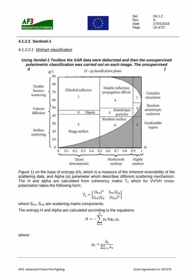
Using Sentiel-1 Toolbox the SAR data were debursted and then the unsupervised polarimetric classification was carried out on each image. The unsupervised divides the H/Alpha plane [Cloude & Pottier, 1997] into 9 scattering zones (

Figure 1) on the base of entropy (H), which is a measure of the inherent reversibility of the scattering data, and Alpha (α) parameter which describes different scattering mechanism. The H and alpha are calculated from coherency matrix T2 which for VV/VH cross-polarization takes the following form:

𝑇2 = [|𝑆𝑉𝑉|2 𝑆𝑉𝑉𝑆𝑉𝐻

∗

𝑆𝑉𝐻𝑆𝑉𝑉∗ |𝑆𝑉𝐻|2 ]

where SVV, SVH are scattering matrix components.

The entropy H and Alpha are calculated according to the equations:

𝐻 = − ∑ 𝑝𝑘 log𝑛 𝑝𝑘

𝑛

𝑘=1

where:

𝑝𝑘 =𝜆𝑘

∑ 𝜆𝑘𝑛𝑘=1

Del. Rev. Date Page

D4.1.2 A 27/01/2016 20 of 37


and λk are eigenvalues of coherence matrix:

𝛼 = ∑ 𝑝𝑘𝛼𝑘

𝑛

𝑘=1

where:

αk = cos−1 |𝑢1𝑘|

and u1k are components of coherence matrix eigenvectros.

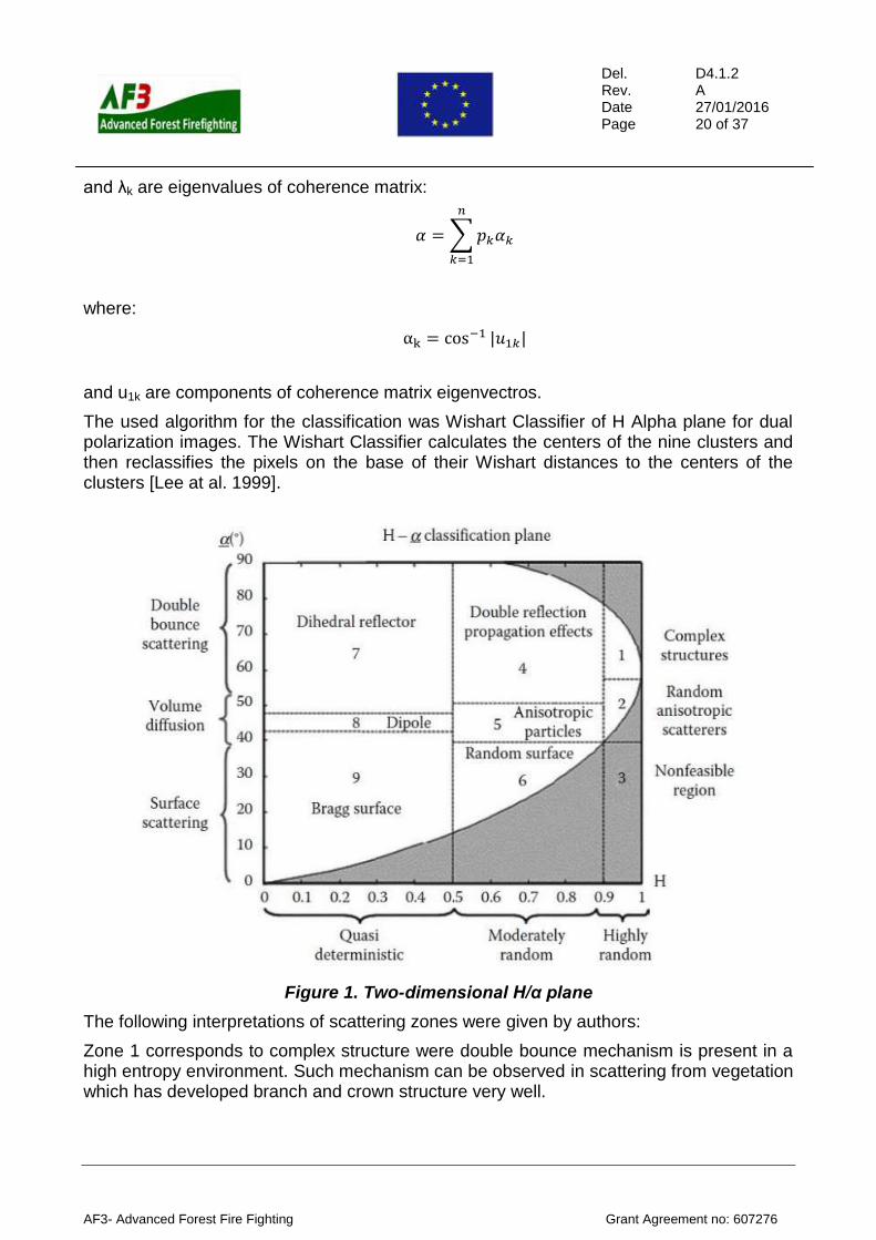
The used algorithm for the classification was Wishart Classifier of H Alpha plane for dual polarization images. The Wishart Classifier calculates the centers of the nine clusters and then reclassifies the pixels on the base of their Wishart distances to the centers of the clusters [Lee at al. 1999].

Figure 1. Two-dimensional H/α plane

The following interpretations of scattering zones were given by authors:

Zone 1 corresponds to complex structure were double bounce mechanism is present in a high entropy environment. Such mechanism can be observed in scattering from vegetation which has developed branch and crown structure very well.

Del. Rev. Date Page

D4.1.2 A 27/01/2016 21 of 37


Zone 2 encloses volume scattering and high entropy. This can arise from cloud of anisotropic needle like particles. This zone can correspond to some types of vegetation surfaces with random highly anisotropic scattering elements.

Zone 3 which corresponds to high entropy and surface scattering is considered no feasible region.

Zone 4 is characterized by dihedral scattering with moderate entropy. This can correspond to surfaces where the double bounce mechanism occurs such as forests or build-up areas.

Zone 5 includes scattering from vegetated surfaces with anisotropic scatters and moderate correlation of scatter orientation.

Zone 6 corresponds with surfaces roughness of a canopy propagation effects.

Zone 7 enclosed isolated dielectric and metallic dihedral scatters.

Zone 8 describes a large imbalance between HH and VV in amplitude. It is connected to isolated dipole scatters such as some kinds of vegetation with strongly correlated orientation of anisotropic scattering elements.

Zone 9 is dedicated to Bragg surface scattering and specular surface scattering as water, sea-ice or very smooth land surfaces.

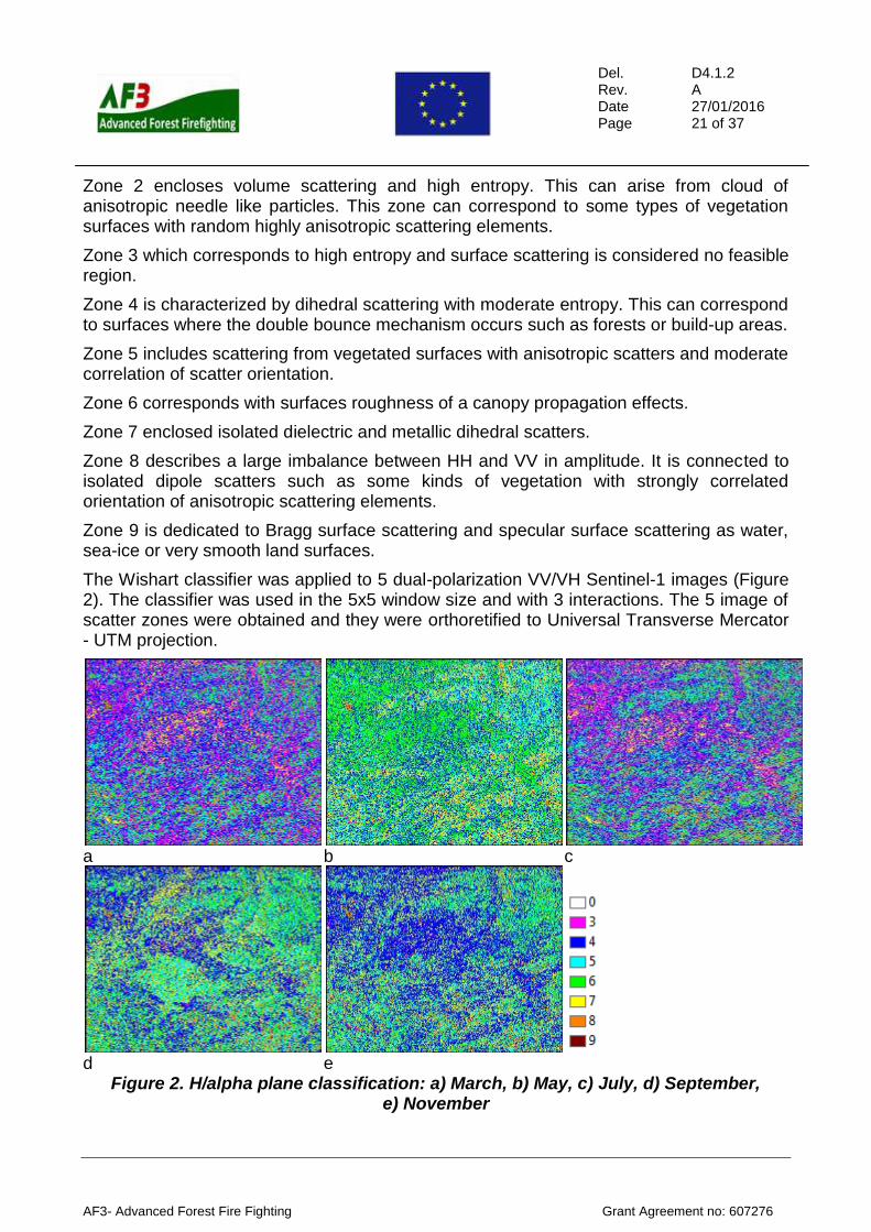
The Wishart classifier was applied to 5 dual-polarization VV/VH Sentinel-1 images (Figure 2). The classifier was used in the 5x5 window size and with 3 interactions. The 5 image of scatter zones were obtained and they were orthoretified to Universal Transverse Mercator - UTM projection.

a b c

d e

Figure 2. H/alpha plane classification: a) March, b) May, c) July, d) September, e) November

Del. Rev. Date Page

D4.1.2 A 27/01/2016 22 of 37


4.1.2.2.2 Multi-temporal analysis

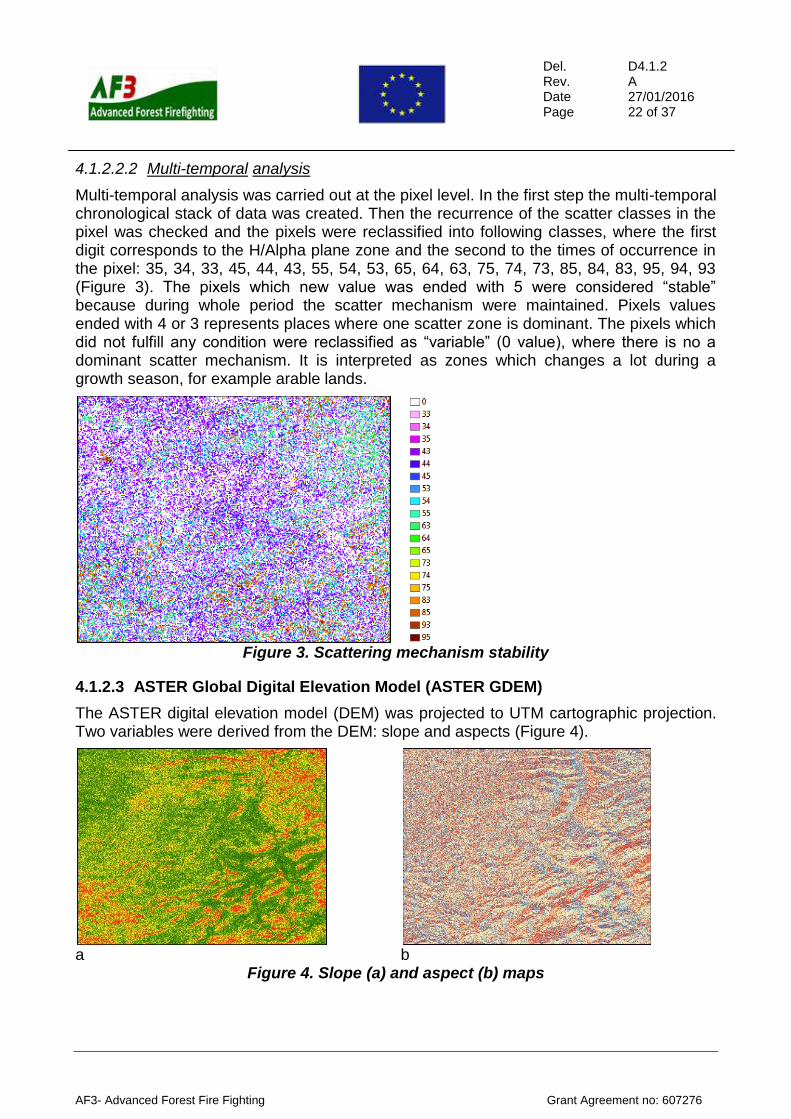
Multi-temporal analysis was carried out at the pixel level. In the first step the multi-temporal chronological stack of data was created. Then the recurrence of the scatter classes in the pixel was checked and the pixels were reclassified into following classes, where the first digit corresponds to the H/Alpha plane zone and the second to the times of occurrence in the pixel: 35, 34, 33, 45, 44, 43, 55, 54, 53, 65, 64, 63, 75, 74, 73, 85, 84, 83, 95, 94, 93 (Figure 3). The pixels which new value was ended with 5 were considered “stable” because during whole period the scatter mechanism were maintained. Pixels values ended with 4 or 3 represents places where one scatter zone is dominant. The pixels which did not fulfill any condition were reclassified as “variable” (0 value), where there is no a dominant scatter mechanism. It is interpreted as zones which changes a lot during a growth season, for example arable lands.

Figure 3. Scattering mechanism stability

4.1.2.3 ASTER Global Digital Elevation Model (ASTER GDEM)

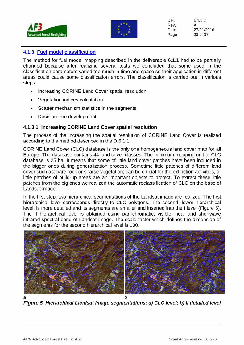
The ASTER digital elevation model (DEM) was projected to UTM cartographic projection. Two variables were derived from the DEM: slope and aspects (Figure 4).

a b

Figure 4. Slope (a) and aspect (b) maps

Del. Rev. Date Page

D4.1.2 A 27/01/2016 23 of 37


4.1.3 Fuel model classification

The method for fuel model mapping described in the deliverable 6.1.1 had to be partially changed because after realizing several tests we concluded that some used in the classification parameters varied too much in time and space so their application in different areas could cause some classification errors. The classification is carried out in various steps:

Increasing CORINE Land Cover spatial resolution

Vegetation indices calculation

Scatter mechanism statistics in the segments

Decision tree development

4.1.3.1 Increasing CORINE Land Cover spatial resolution

The process of the increasing the spatial resolution of CORINE Land Cover is realized according to the method described in the D 6.1.1.

CORINE Land Cover (CLC) database is the only one homogeneous land cover map for all Europe. The database contains 44 land cover classes. The minimum mapping unit of CLC database is 25 ha. It means that some of little land cover patches have been included in the bigger ones during generalization process. Sometime little patches of different land cover such as: bare rock or sparse vegetation; can be crucial for the extinction activities, or little patches of build-up areas are an important objects to protect. To extract these little patches from the big ones we realized the automatic reclassification of CLC on the base of Landsat image.

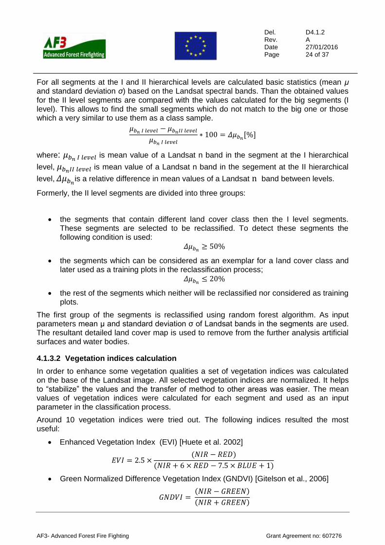
In the first step, two hierarchical segmentations of the Landsat image are realized. The first hierarchical level corresponds directly to CLC polygons. The second, lower hierarchical level, is more detailed and its segments are smaller and inserted into the I level (Figure 5). The II hierarchical level is obtained using pan-chromatic, visible, near and shortwave infrared spectral band of Landsat image. The scale factor which defines the dimension of the segments for the second hierarchical level is 100.

a b Figure 5. Hierarchical Landsat image segmentations: a) CLC level; b) II detailed level

Del. Rev. Date Page

D4.1.2 A 27/01/2016 24 of 37


For all segments at the I and II hierarchical levels are calculated basic statistics (mean μ and standard deviation σ) based on the Landsat spectral bands. Than the obtained values for the II level segments are compared with the values calculated for the big segments (I level). This allows to find the small segments which do not match to the big one or those which a very similar to use them as a class sample.

𝜇𝑏𝑛 𝐼 𝑙𝑒𝑣𝑒𝑙 − 𝜇𝑏𝑛𝐼𝐼 𝑙𝑒𝑣𝑒𝑙

𝜇𝑏𝑛 𝐼 𝑙𝑒𝑣𝑒𝑙∗ 100 = 𝛥𝜇𝑏𝑛

[%]

where: 𝜇𝑏𝑛 𝐼 𝑙𝑒𝑣𝑒𝑙 is mean value of a Landsat n band in the segment at the I hierarchical

level, 𝜇𝑏𝑛𝐼𝐼 𝑙𝑒𝑣𝑒𝑙 is mean value of a Landsat n band in the segement at the II hierarchical

level, 𝛥𝜇𝑏𝑛is a relative difference in mean values of a Landsat n band between levels.

Formerly, the II level segments are divided into three groups:

the segments that contain different land cover class then the I level segments. These segments are selected to be reclassified. To detect these segments the following condition is used:

𝛥𝜇𝑏𝑛≥ 50%

the segments which can be considered as an exemplar for a land cover class and later used as a training plots in the reclassification process;

𝛥𝜇𝑏𝑛≤ 20%

the rest of the segments which neither will be reclassified nor considered as training plots.

The first group of the segments is reclassified using random forest algorithm. As input parameters mean μ and standard deviation σ of Landsat bands in the segments are used. The resultant detailed land cover map is used to remove from the further analysis artificial surfaces and water bodies.

4.1.3.2 Vegetation indices calculation

In order to enhance some vegetation qualities a set of vegetation indices was calculated on the base of the Landsat image. All selected vegetation indices are normalized. It helps to “stabilize” the values and the transfer of method to other areas was easier. The mean values of vegetation indices were calculated for each segment and used as an input parameter in the classification process.

Around 10 vegetation indices were tried out. The following indices resulted the most useful:

Enhanced Vegetation Index (EVI) [Huete et al. 2002]

𝐸𝑉𝐼 = 2.5 ×(𝑁𝐼𝑅 − 𝑅𝐸𝐷)

(𝑁𝐼𝑅 + 6 × 𝑅𝐸𝐷 − 7.5 × 𝐵𝐿𝑈𝐸 + 1)

Green Normalized Difference Vegetation Index (GNDVI) [Gitelson et al., 2006]

𝐺𝑁𝐷𝑉𝐼 = (𝑁𝐼𝑅 − 𝐺𝑅𝐸𝐸𝑁)

(𝑁𝐼𝑅 + 𝐺𝑅𝐸𝐸𝑁)

Del. Rev. Date Page

D4.1.2 A 27/01/2016 25 of 37


Infrared Percentage Vegetation Index (IPVI) [Crippen, 1990]

𝐼𝑃𝑉𝐼 = 𝑁𝐼𝑅

𝑁𝐼𝑅 + 𝑅𝐸𝐷

Modified Normalized Difference (MND) [Paltridge & Barber, 1988]

𝑀𝑁𝐷 = 𝑁𝐼𝑅 − (1.2 × 𝑅𝐸𝐷)


Visible Atmospherically Resistant Index (VARI) [Gitelson et al., 2002]

𝑉𝐴𝑅𝐼 = 𝐺𝑅𝐸𝐸𝑁 − 𝑅𝐸𝐷

𝐺𝑅𝐸𝐸𝑁 + 𝑅𝐸𝐷 − 𝐵𝐿𝑈𝐸

4.1.3.3 Scatter mechanism statistics in the segments

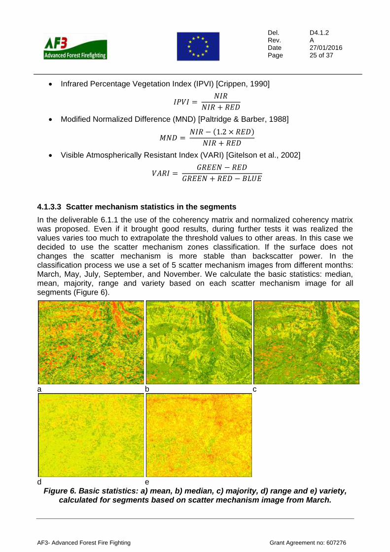
In the deliverable 6.1.1 the use of the coherency matrix and normalized coherency matrix was proposed. Even if it brought good results, during further tests it was realized the values varies too much to extrapolate the threshold values to other areas. In this case we decided to use the scatter mechanism zones classification. If the surface does not changes the scatter mechanism is more stable than backscatter power. In the classification process we use a set of 5 scatter mechanism images from different months: March, May, July, September, and November. We calculate the basic statistics: median, mean, majority, range and variety based on each scatter mechanism image for all segments (Figure 6).

a b c

d e Figure 6. Basic statistics: a) mean, b) median, c) majority, d) range and e) variety,

calculated for segments based on scatter mechanism image from March.

Del. Rev. Date Page

D4.1.2 A 27/01/2016 26 of 37


The same statistics were computed for all segments based on the multi-temporal scattering mechanism stability.

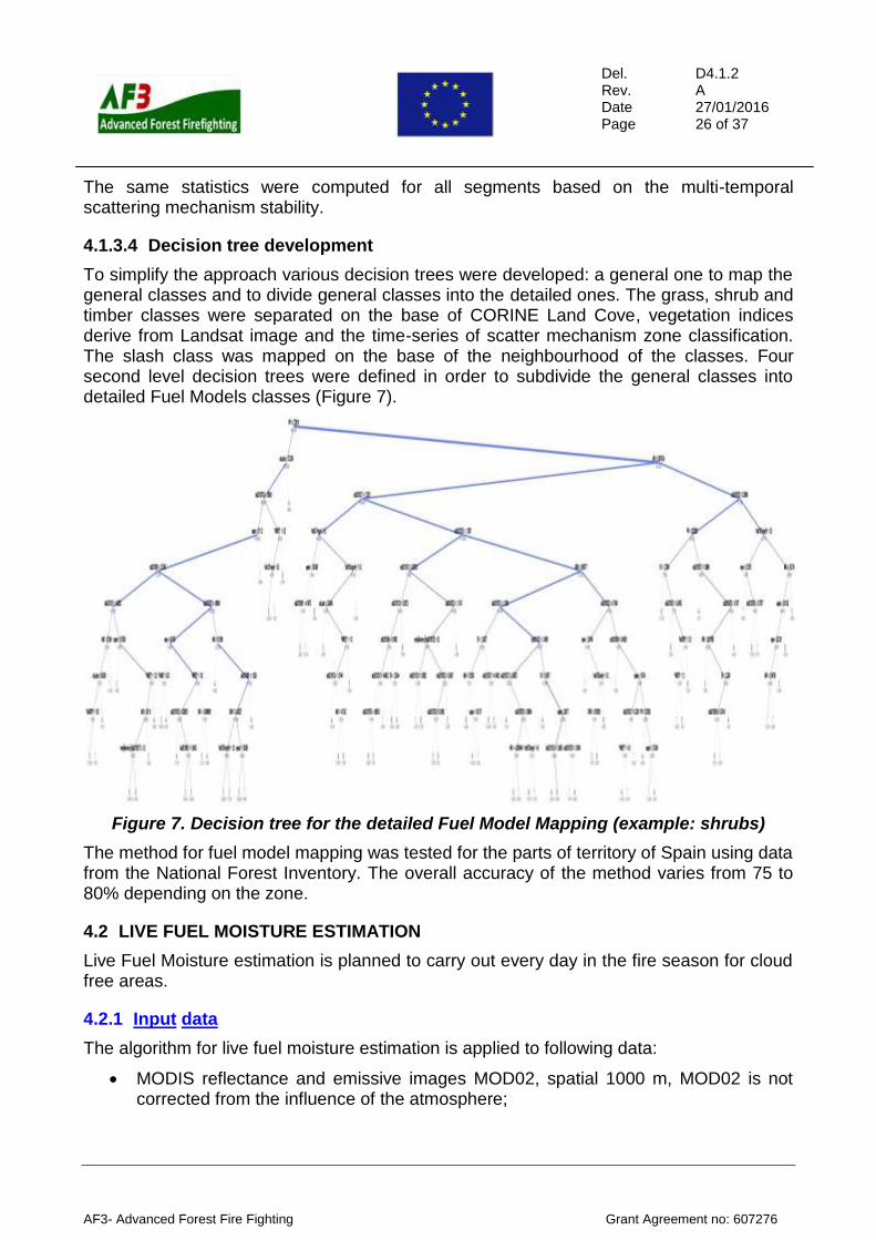
4.1.3.4 Decision tree development

To simplify the approach various decision trees were developed: a general one to map the general classes and to divide general classes into the detailed ones. The grass, shrub and timber classes were separated on the base of CORINE Land Cove, vegetation indices derive from Landsat image and the time-series of scatter mechanism zone classification. The slash class was mapped on the base of the neighbourhood of the classes. Four second level decision trees were defined in order to subdivide the general classes into detailed Fuel Models classes (Figure 7).

Figure 7. Decision tree for the detailed Fuel Model Mapping (example: shrubs)

The method for fuel model mapping was tested for the parts of territory of Spain using data from the National Forest Inventory. The overall accuracy of the method varies from 75 to 80% depending on the zone.

4.2 LIVE FUEL MOISTURE ESTIMATION

Live Fuel Moisture estimation is planned to carry out every day in the fire season for cloud free areas.

4.2.1 Input data

The algorithm for live fuel moisture estimation is applied to following data:

MODIS reflectance and emissive images MOD02, spatial 1000 m, MOD02 is not corrected from the influence of the atmosphere;

Del. Rev. Date Page

D4.1.2 A 27/01/2016 27 of 37


MODIS reflectance images MOD9, spatial resolution of 500 m, MOD09 image is corrected from the influence of the atmosphere;

MODIS cloud mask MOD35 product, spatial resolution of 1000 m;

CORINE Land Cover database.

4.2.2 Method

As it was describe in the deliverable 6.1.1 the live fuel moisture content is estimated according to Chuvieco et al. algorithm [2004]. The algorithm is a function of Land Surface Temperature (LST), Normalized Difference Vegetation Index (NDVI) and day of the year (FD). It is calculated separately for herbaceous (FMCh) and woody/shrub (FMCs) vegetation:

𝐹𝑀𝐶ℎ = −57,103 + 284,88 × 𝑁𝐷𝑉𝐼 − 0,089 × 𝐿𝑆𝑇 + 136,75 × 𝐹𝐷ℎ

𝐹𝑀𝐶𝑠 = 70,195 + 53,520 × 𝑁𝐷𝑉𝐼 − 1,435 × 𝐿𝑆𝑇 + 122,087 × 𝐹𝐷𝑠

The Normalized Difference Vegetation Index (NDVI) [Rouse at al. 1974], which is an input variable to FMC calculation, is obtained from MODIS MOD9 product using following equation:

𝑁𝐷𝑉𝐼 =𝑁𝐼𝑅 − 𝑅𝐸𝐷


The next variable in the FMC equation is Land Surface Temperature (LST). To calculate LST the Water Vapour (WV) has to be estimated firstly. WV and LST are calculated according to the Sobrino et al. [2003] algorithm using MOD02 images.

To calculate the water vapour, the ratios between absorption (b2) and transmission (b17, b18, b19) bands are computed:

𝐺17 =𝑏17

𝑏2

𝐺18 =𝑏18

𝑏2

𝐺19 =𝑏19

𝑏2

where: b2, b17, b18, b19 are MODIS bands

Then water vapour content is calculated for each band and the final water vapour content is a weighted sum of estimations computed for each band:

𝑊17 = 26,314 − 54,434𝐺17 + 28,449𝐺172

𝑊18 = 5,012 − 23,017𝐺18 + 27,884𝐺182

𝑊19 = 9,446 − 25,887𝐺19 + 19,914𝐺192

𝑊 = 0,192𝑊17 + 0,453𝑊18 + 0,355𝑊19

The LST is calculated according to the equation:

𝑇𝐿𝑆𝑇 = 𝑇31 + 1,02 + 1,79(𝑇31 − 𝑇32) + 1,2(𝑇31 − 𝑇32)2 + (34,83— 0,68𝑊)(1 − 𝜀) − (73,27+ 5,19𝑊)∆𝜀

Del. Rev. Date Page

D4.1.2 A 27/01/2016 28 of 37


where: T31, T32 are the brightness temperature calculated from MODIS bands 31 and 32; W is water vapour, ε is emissivity of vegetation.

The last variable in the FMC equation is function of the day (FD) of the year (Dy) which has a following form:

𝐹𝐷ℎ = (sin (1,5 × 𝜋 ×𝐷𝑦 + 𝐷𝑦

13⁄

365)4) × 1,3

𝐹𝐷𝑠 = (sin (1,5 × 𝜋 × (𝐷𝑦

365))2 + 1) × 0,35

According to the authors the estimation of the coefficient of determination of the function R2 for grassland varies from 0,88 to 0,91 and for shrubs the R2 is 0,85.

Del. Rev. Date Page

D4.1.2 A 27/01/2016 29 of 37


5. SOFTWARE DESCRIPTION

5.1 FMM PREPROCESSING SOFTWARE

Software implementing the method can be run on Windows or Linux (OS X is untested). Pre configuration is required and is achieved via config files. Application can be run manually or automatically, using an automated task manager (ex. cron on Linux). Java Runtime Environment and Python need to be installed before use. Both can be freely downloaded for the Internet.

5.1.1 Software Requirements

You need to install the following packages. They may already be installed on your system.

Java Runtime Environment

Download from here: https://www.java.com/en/download/

Python 2.7

Download from here: https://www.python.org/downloads/

On Linux, equivalent packages can also be found in distribution repositories.

5.1.2 Pre-configuration

5.1.2.1 Data access

To use the application, you need to acquire the satellite images. You need to obtain the credentials for online data access.

SciHub for Sentinel data

https://scihub.copernicus.eu

USGS EROS Registration System for Landsat data

https://ers.cr.usgs.gov/register/

Put the username and password, separated by a single space (ex. 'username password', without quotes) in a single line into the proper config file:

scihub.txt for SciHub

usgs.txt for EROS

5.1.2.2 Area of interest configuration

The area of interest is configured based on a geospatial file in geojson format. This file needs to be called aoi.geojson and needs to have the following structure: {

"type": "FeatureCollection",

"features": [

{ "type": "Feature",

"properties": { "key": "value"},

"geometry": { "type": "Polygon",

https://www.java.com/en/download/

https://www.python.org/downloads/

https://scihub.copernicus.eu/

https://ers.cr.usgs.gov/register/

Del. Rev. Date Page

D4.1.2 A 27/01/2016 30 of 37


"coordinates": [ [ [21.016667, 52.233333], [21.116667,

52.233333], [21.116667, 52.333333], [21.016667, 52.333333], [21.016667,

52.233333] ] ] }

}

]

}

Values of: properties.name features[0].geometry.properties features[0].geometry.coordinates

are example values.

The coordinates need to be in lon-lat format.

The presented geojson format is the default format from a conversion of a shapefile using ogr2ogr utility from GDAL/OGR package.

5.1.3 Running the application

5.1.3.1 Manually

You can run the application by double-clicking on the java binary af3_FMM.jar. This will result in the application running with default settings, as defined in default.txt.

You can also run the application from command line interface (CLI), with the following options: -sd Start date -ed End date -cp Password config dir -cf config file (overrides other cli parameters) -aoi aoi geojson file -dd data dir

examples: java -jar af3_FMM.jar -sd 20150101 -ed 20151231 -cp ../config -aoi ../config/aoi.geojson java -jar af3_FMM.jar -cf ../config/default.txt default.txt is a config text file, where you can write the switches, just like on cli, example: -sd 20150101 -ed 20151231 -cp ../config -aoi ../config/aoi.geojson

By using the '-dd' option, you can specify the directory, where the source data (satellite imagery) is. Using this option stops the application from downloading data from the internet and the data found in the directory is used instead.

5.1.3.2 Automatically

Windows: documentation on how to run tasks with Windows Task Scheduler can be found here: https://msdn.microsoft.com/en-us/library/aa383614.aspx

Linux: crontab documentation can be found here:

http://pubs.opengroup.org/onlinepubs/9699919799/utilities/crontab.html

https://msdn.microsoft.com/en-us/library/aa383614.aspx

Del. Rev. Date Page

D4.1.2 A 27/01/2016 31 of 37


5.2 FMM LIBRARY

The FMM Library encloses described above Fuel Model Map algorithm. The software returns raster data in geotiff format, which contain Fuel Model Map.


To run “Fuel Model Map” algorithm, installation of eCognition Architect or eCognition Developer (version 9.1.3; Build 2918 x64 or newer) is required.

5.2.1.1 Input Data

Given below is the list of all input files required for the further processing.

List of input raster files

Landsat multispectral image

Landsat panchromatic image

Sentinel - 2 multispectral image

Scatter image for times T1 – T5

Multitemporal scatter image

Aspect image

Slope image

List of input vector files

Corine Land Cover

Scatter Statistics

Multitemporal Scatter Statistics

Fire history

5.2.1.2 Opening Action Library in eCognition

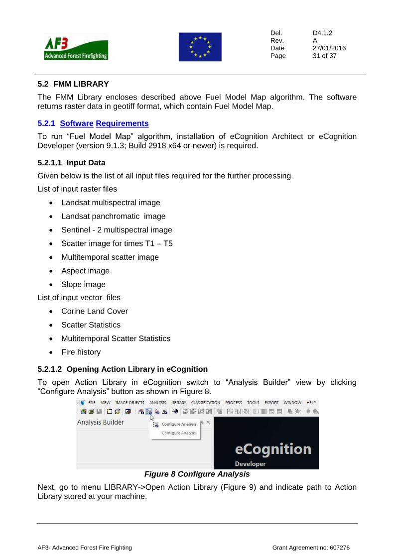
To open Action Library in eCognition switch to “Analysis Builder” view by clicking “Configure Analysis” button as shown in Figure 8.

Figure 8 Configure Analysis

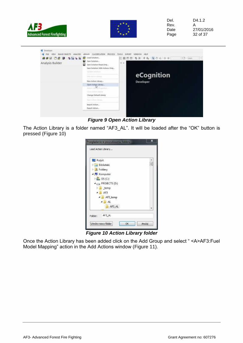
Next, go to menu LIBRARY->Open Action Library (Figure 9) and indicate path to Action Library stored at your machine.

Del. Rev. Date Page

D4.1.2 A 27/01/2016 32 of 37


Figure 9 Open Action Library

The Action Library is a folder named “AF3_AL”. It will be loaded after the “OK” button is pressed (Figure 10)

Figure 10 Action Library folder

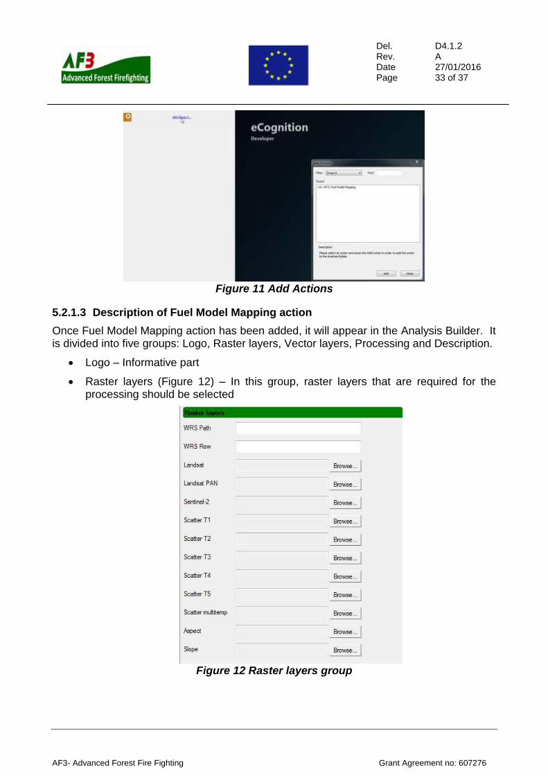
Once the Action Library has been added click on the Add Group and select “ <A>AF3:Fuel Model Mapping” action in the Add Actions window (Figure 11).

Del. Rev. Date Page

D4.1.2 A 27/01/2016 33 of 37


Figure 11 Add Actions

5.2.1.3 Description of Fuel Model Mapping action

Once Fuel Model Mapping action has been added, it will appear in the Analysis Builder. It is divided into five groups: Logo, Raster layers, Vector layers, Processing and Description.

Logo – Informative part

Raster layers (Figure 12) – In this group, raster layers that are required for the processing should be selected

Figure 12 Raster layers group

Del. Rev. Date Page

D4.1.2 A 27/01/2016 34 of 37


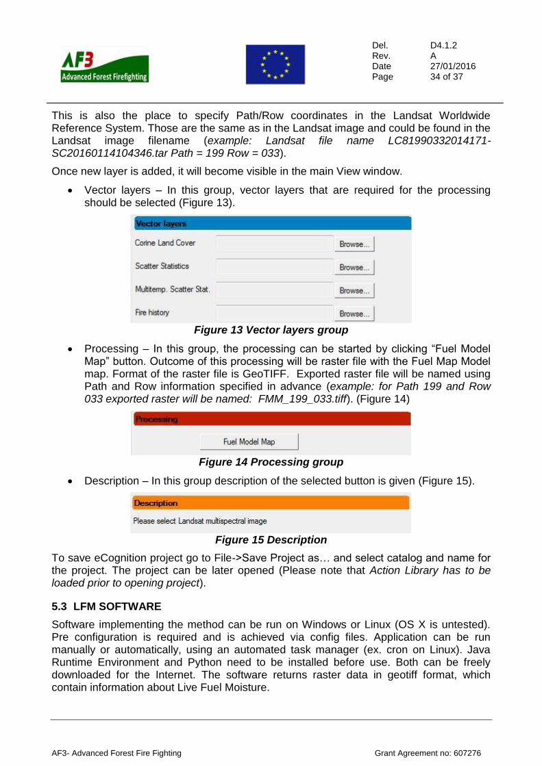
This is also the place to specify Path/Row coordinates in the Landsat Worldwide Reference System. Those are the same as in the Landsat image and could be found in the Landsat image filename (example: Landsat file name LC81990332014171-SC20160114104346.tar Path = 199 Row = 033).

Once new layer is added, it will become visible in the main View window.

Vector layers – In this group, vector layers that are required for the processing should be selected (Figure 13).

Figure 13 Vector layers group

Processing – In this group, the processing can be started by clicking “Fuel Model Map” button. Outcome of this processing will be raster file with the Fuel Map Model map. Format of the raster file is GeoTIFF. Exported raster file will be named using Path and Row information specified in advance (example: for Path 199 and Row 033 exported raster will be named: FMM_199_033.tiff). (Figure 14)

Figure 14 Processing group

Description – In this group description of the selected button is given (Figure 15).

Figure 15 Description

To save eCognition project go to File->Save Project as… and select catalog and name for the project. The project can be later opened (Please note that Action Library has to be loaded prior to opening project).

5.3 LFM SOFTWARE

Software implementing the method can be run on Windows or Linux (OS X is untested). Pre configuration is required and is achieved via config files. Application can be run manually or automatically, using an automated task manager (ex. cron on Linux). Java Runtime Environment and Python need to be installed before use. Both can be freely downloaded for the Internet. The software returns raster data in geotiff format, which contain information about Live Fuel Moisture.

Del. Rev. Date Page

D4.1.2 A 27/01/2016 35 of 37



You need to install the following packages. They may already be installed on your system.

Java Runtime Environment

Download from here: https://www.java.com/en/download/

Python 2.7

Download from here: https://www.python.org/downloads/

On Linux, equivalent packages can also be found in distribution repositories.

5.3.2 Pre-configuration

5.3.2.1 Data access

To use the application, you need to acquire the satellite images. You need to obtain the credentials for online data access.

LANCE for MODIS data

https://urs.earthdata.nasa.gov/users/new

Put the username and password, separated by a single space (ex. 'username password', without quotes) in a single line into the proper config file:

lance.txt for LANCE

5.3.2.2 Area of interest configuration

The area of interest is configured based on a geospatial file in geojson format. This file needs to be called aoi.geojson and needs to have the following structure: {

"type": "FeatureCollection",

"features": [

{ "type": "Feature",

"properties": { "key": "value"},

"geometry": { "type": "Polygon",

"coordinates": [ [ [21.016667, 52.233333], [21.116667,

52.233333], [21.116667, 52.333333], [21.016667, 52.333333], [21.016667,

52.233333] ] ] }

}

]

}

Values of: properties.name features[0].geometry.properties features[0].geometry.coordinates

are example values.

The coordinates need to be in lon-lat format.

The presented geojson format is the default format from a conversion of a shapefile using ogr2ogr utility from GDAL/OGR package.

https://www.java.com/en/download/

https://www.python.org/downloads/

Del. Rev. Date Page

D4.1.2 A 27/01/2016 36 of 37


5.3.3 Running the application

5.3.3.1 Manually

You can run the application by double-clicking on the java binary af3_LFM.jar. This will result in the application running with default settings, as defined in default.txt.

You can also run the application from command line interface (CLI), with the following options: -sd Start date -ed End date -cp Password config dir -cf config file (overrides other cli parameters) -aoi aoi geojson file -dd data dir

examples: java -jar af3_LFM.jar -sd 20150101 -ed 20151231 -cp ../config -aoi ../config/aoi.geojson java -jar af3_LFM.jar -cf ../config/default.txt

default.txt is a config text file, where you can write the switches, just like on cli, example:

-sd 20150101 -ed 20151231 -cp ../config -aoi ../config/aoi.geojson

By using the '-dd' option, you can specify the directory, where the source data (satellite imagery) is. Using this option stops the application from downloading data from the internet and the data found in the directory is used instead.

5.3.3.2 Automatically

Windows: documentation on how to run tasks with Windows Task Scheduler can be found here: https://msdn.microsoft.com/en-us/library/aa383614.aspx Linux: crontab documentation can be found here: http://pubs.opengroup.org/onlinepubs/9699919799/utilities/crontab.html

https://msdn.microsoft.com/en-us/library/aa383614.aspx

http://pubs.opengroup.org/onlinepubs/9699919799/utilities/crontab.html

Del. Rev. Date Page

D4.1.2 A 27/01/2016 37 of 37


6. CONCLUSIONS

The aims of the WP 4.1 task 4.1.2.” Distribution analysis of the vegetation” were to determine the spatial distribution of fuel types and estimate the fuel moisture. The objectives were archived. The fuels were classified according to NFFL fuel model system with the overall accuracy of 75-80%. The fuel model map is designed to be updated once per year. The fuel model map can be easily converted to fire load values according the NFFL fuel description. The function for the estimation of live fuel moisture has determination coefficient 0,88 for grass and 0,85 for shrubs. The live fuel moisture product is updated every day for cloud free areas.

Following software was developed:

For downloading and pre-processing Landsat and Sentinel data. This software prepares all inputs to the Fuel Model Mapping software;

For Fuel Model Mapping. The software encloses the classification algorithm;

For Fuel Moisture estimation. The software automatically downloads and pre-processes MODIS data, as well as it applies the Life Fuel Moisture algorithm.

All software returns data in geotiff format. Only FMM software is dedicated to one specific algorithm. The Santinel-1 and Landsat pre-processing software and LFM software can be used for other proposes in the project, for example: burnt area mapping.

af3 advanced forest fire fighting -...

Documents