Aerospace Defense Symposium

Adaptive EW simulation

Walt SchulteApplications engineer: MCDPresented by:Steve SanelliSenior RF/uW Applications Engineer

Agenda

• Basic EW• EW test• Multi-emitter simulation• Closed-loop adaptive simulation

The threat environmentEarly warning (VHF - S-band)

Engagement, fire control (C – Ku band)

Fire Control

Pu

lse

Den

sity

(p

ps)

VHF UHF L S C X Ku

B C D E F G H I JA

Early Warning

Acq, Grnd Cntrl Intercept

106

105

104

103

102

101

Frequency Bands

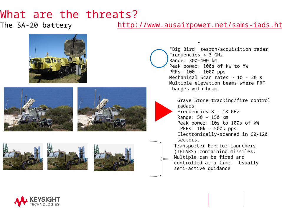
What are the threats?The SA-20 battery

“Big Bird” search/acquisition radarFrequencies < 3 GHzRange: 300-400 kmPeak power: 100s of kW to MWPRFs: 100 – 1000 ppsMechanical Scan rates ~ 10 - 20 sMultiple elevation beams where PRF changes with beam

Grave Stone tracking/fire control radarsFrequencies 8 – 18 GHzRange: 50 – 150 kmPeak power: 10s to 100s of kW PRFs: 10k – 500k ppsElectronically-scanned in 60-120 sectors.

Transporter Erector Launchers (TELARS) containing missiles. Multiple can be fired and controlled at a time. Usually semi-active guidance

http://www.ausairpower.net/sams-iads.html

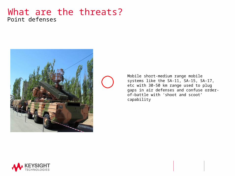
What are the threats?Point defenses

Mobile short-medium range mobile systems like the SA-11, SA-15, SA-17, etc with 30-50 km range used to plug gaps in air defenses and confuse order-of-battle with ‘shoot and scoot’ capability

7

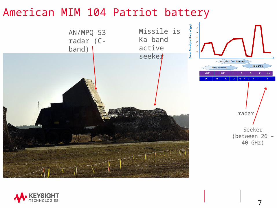
American MIM 104 Patriot battery

AN/MPQ-53 radar (C-band)

Missile is Ka band active seeker

radar

Seeker (between 26 – 40 GHz)

heading

1.

2.

3.

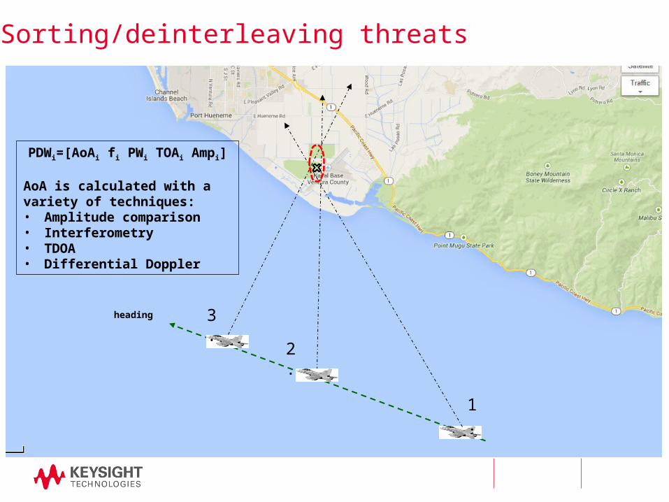
Sorting/deinterleaving threats

PDWi=[AoAi fi PWi TOAi Ampi]

AoA is calculated with a variety of techniques:• Amplitude comparison • Interferometry• TDOA• Differential Doppler

The threat environmentEarly warning (VHF - S-band)

Engagement, fire control (C – Ku band)

headingDOA

20

1520

Integrated EW systemd

Jammer Block Diagram

Fwd Tx Aperture(s)

Aft Tx Aperture(s)

Fwd Rx Aperture(s)

Aft Rx Aperture(s)

Exciter: Frequency synthesis

Techniques generator: DRFM range and velocity offsets

Dig

ita

l re

ce

ive

r

(0-4

0 G

Hz

pu

lse

p

ara

me

teriz

atio

n)

Sorter: sort PDWs into

different emitters by

frequency and AoA

Tracker: identify against MDF, prevent ID’d emitters from re-

entering sorting process, track the mode, control TG

accordingly

PDWs

Co

ntr

ol

wo

rds

RF IF or BB Digital

Si=

[AoA

i fi P

wi T

OA

i Am

p i]

Vi=[AoAi fi ]

incoming threat pulses

outgoing jamming pulses

RF pulses become PDWs

Agenda

• Basic EW• EW test• Multi-emitter simulation• Closed-loop adaptive simulation

High-level RF/uWave test requirements

– 1 to 10 million pulses-per-second

– Agile amplitude range

– Agile frequency switching

– AoA

– Interferers

– Hours-long scenarios simulating EOB

– Adaptivity: change the threats in response to positive tracking and/or jamming from the EW system under test

12

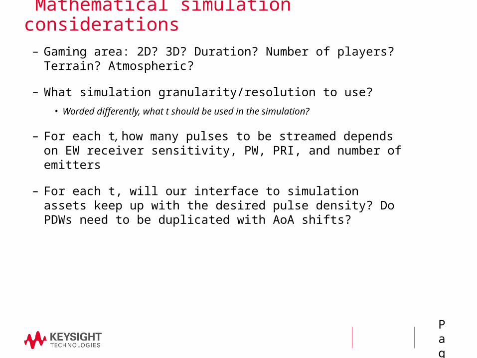
Mathematical simulation considerations– Gaming area: 2D? 3D? Duration? Number of players? Terrain?

Atmospheric?

– What simulation granularity/resolution to use?

• Worded differently, what t should be used in the simulation?

– For each t, how many pulses to be streamed depends on EW receiver sensitivity, PW, PRI, and number of emitters

– For each t, will our interface to simulation assets keep up with the desired pulse density? Do PDWs need to be duplicated with AoA shifts?

Page 13

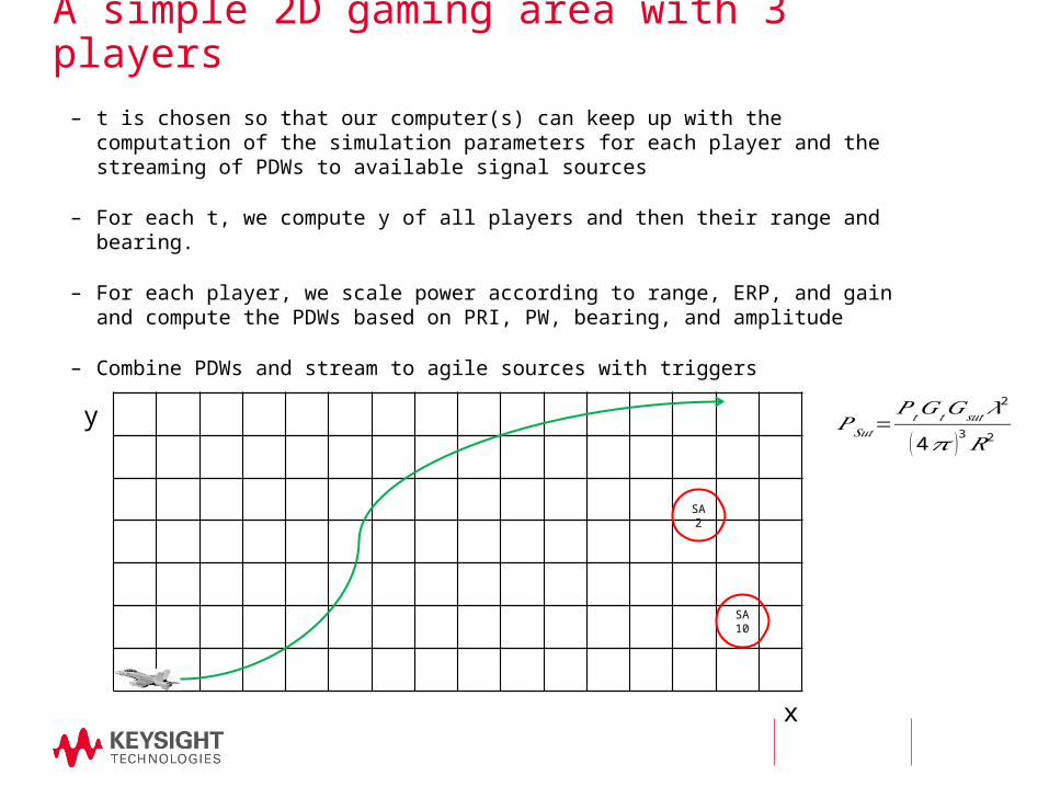
A simple 2D gaming area with 3 players– t is chosen so that our computer(s) can keep up with the computation of the simulation

parameters for each player and the streaming of PDWs to available signal sources

– For each t, we compute y of all players and then their range and bearing.

– For each player, we scale power according to range, ERP, and gain and compute the PDWs based on PRI, PW, bearing, and amplitude

– Combine PDWs and stream to agile sources with triggers

SA2

SA10

𝑃𝑆𝑢𝑡=𝑃 𝑡𝐺𝑡𝐺𝑠𝑢𝑡 𝜆

2

(4𝜋 )3𝑅2

x

y

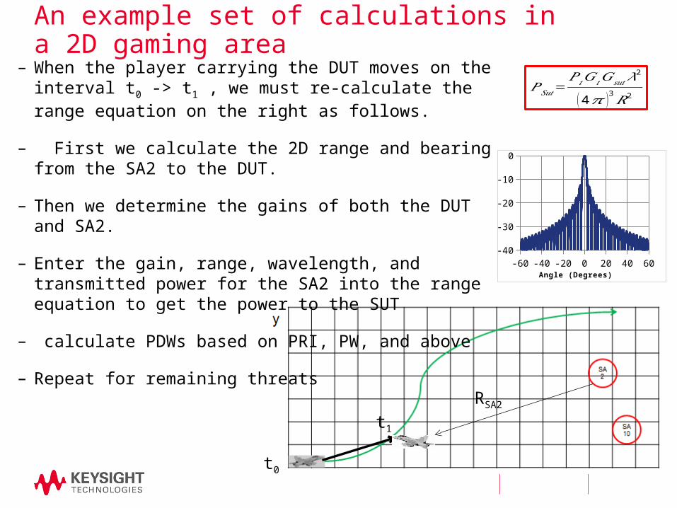
An example set of calculations in a 2D gaming area– When the player carrying the DUT moves on the interval t0 ->

t1 , we must re-calculate the range equation on the right as follows.

– First we calculate the 2D range and bearing from the SA2 to the DUT.

– Then we determine the gains of both the DUT and SA2.

– Enter the gain, range, wavelength, and transmitted power for the SA2 into the range equation to get the power to the SUT

– calculate PDWs based on PRI, PW, and above

– Repeat for remaining threats

𝑃𝑆𝑢𝑡=𝑃 𝑡𝐺𝑡𝐺𝑠𝑢𝑡 𝜆

2

(4𝜋 )3𝑅2

t1

RSA2

-60 -40 -20 0 20 40 60-40-35-30-25-20-15-10-50

Angle (Degrees)

t0

EW test requirements for signal generators

Requirement

– Plays PDWs streams

– Power: precisely controlling 1-way range equation to EW SUT (polarization, range, kinematics, threat Tx, EW SUT Rx)

– Modulation: simulating the threat’s output waveforms

– SPURS, harmonics, images: the EW receiver will try classify all spurious content from 2-18 GHz

Example

– Create scenarios lasting hours or longer

– chirp deviation, Barker chip width

– Less than -70 dBc

EW test requirements for signal generators

Requirement

– Timing resolution: Creating precise pulse widths, PRFs, and DTOA is very important.

– Switching speed: creating maximum pulse density with the minimum number of signal generators

– Create Angle of Arrival (AoA)

– ~2 ns timing resolution for adjusting PRI and pulse width

– Switching speeds of ~ 200 ns

– Multi-source synchronization for <10 ps DTOA, <1ₒ phase, <.1 dB amplitude

Example

20 and 40 GHz OptionsFor high-speed, low phase noise, multi-port applications

• 200 ns update rate•Phase repeatable or phase continuous frequency switching• Two Amplitude Ranges

• 10 dBM LO • -120 to 0 dBm (90 dB agile)

• 10-25% Linear Chirp Widths• Arbitrary Chirp Profiles

• Pulse ~6 nS Rise/ Fall Pulses, 90 dB on/off• -70 dBc spurious @18 GHz • Industry leading phase noise -126 dBc @10 kHz @10 GHz• Multiple Instrument Coherence

Lower cost of ownership• Industry’s best reliability with a target MTBF of 75k hours.

UXG Agile Signal Generator

Frequency Range 0.01 to 20/40 GHz

Output Power + 10 dBm

Agile Amplitude Switching Range

80 dB < 0 dBM20 GHz Model Only

Agile Amplitude Switching Range

10 dB >0 dBM

Phase Noise (10 GHz @ 20 kHz offset (typical)

-126 dBc/Hz

Non-harmonic Spurious

-70 dBc

Digital word control Frequency, FM/PM

Compatibility mode Comstron

Pulse On/Off 90 db

Minimum Pulse Width

5nS

Size 3U

Page 19

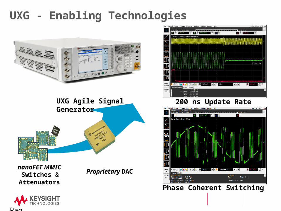
nanoFET MMIC Switches & Attenuators

Proprietary DAC

200 ns Update Rate

Phase Coherent Switching

UXG Agile Signal Generator

UXG - Enabling Technologies

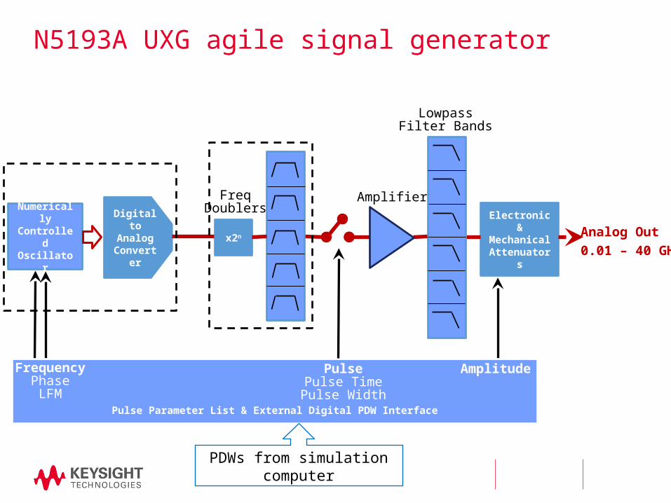
NumericallyControlledOscillator

Electronic &MechanicalAttenuators

Analog Out

0.01 – 40 GHz

Digital toAnalog

Converterx2n

FreqDoublers

LowpassFilter Bands

Amplifier

Pulse Parameter List & External Digital PDW Interface

FrequencyPhaseLFM

PulsePulse TimePulse Width

Amplitude

N5193A UXG agile signal generator

PDWs from simulation computer

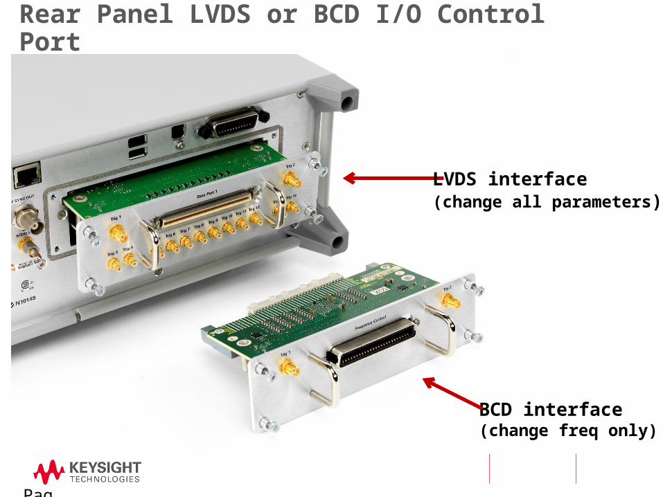
Rear Panel LVDS or BCD I/O Control Port

Page 21

BCD interface(change freq only)

LVDS interface(change all parameters)

Keysight ConfidentialJuly 2014

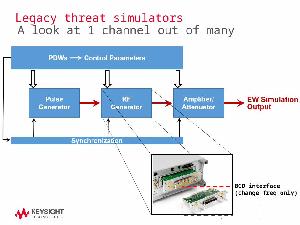
Legacy threat simulatorsA look at 1 channel out of many

BCD interface(change freq only)

Threat simulation todayA look at 1 channel out of many

LVDS interface(send PDWs, source replaces all other simulation elements)Threat simulation

computer

PDWs

Agenda

• Basic EW• EW test• Multi-emitter simulation• Closed-loop adaptive simulation

Creating pulse density

– What is pulse-on-pulse?

– Pulse collisions depend not only on number of emitters but also their PRFs, PWs and therefore duty cycles.

vs

Low PRF emitter density vs Pulse Collision Percentage

Pul

se C

ollis

ion

Per

cent

age

Millions of pulses per second Millions of pulses per second

Pul

se C

ollis

ion

Per

cent

age

High PRF emitter density vs Pulse Collision Percentage

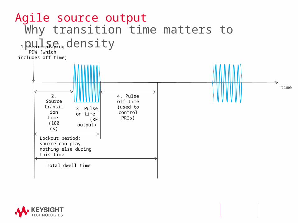
2. Source transition

time (180 ns)

Agile source output Why transition time matters to pulse density

1. Start playing PDW (which includes off time)

3. Pulse on time

(RF output)

Lockout period: source can play nothing else during this time

time

4. Pulse off time (used to control PRIs)

Total dwell time

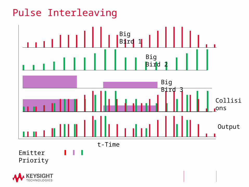
Pulse Interleaving

t-TimeEmitter Priority

Big Bird 1

Big Bird 2

Big Bird 3

Collisions

Output

Creating AoA to test sorting

– The digital receiver parameterizes the RF pulse into a PDW

– Each PDW is [AoAi fi PWi TOAi Ampi]

– AoA and frequency are primary sorting parameters

– Simulation must create AoA at RF!

φ0∆ 𝑡 1 , φ1∆ 𝑡 2 , φ2∆ 𝑡 3 , φ3

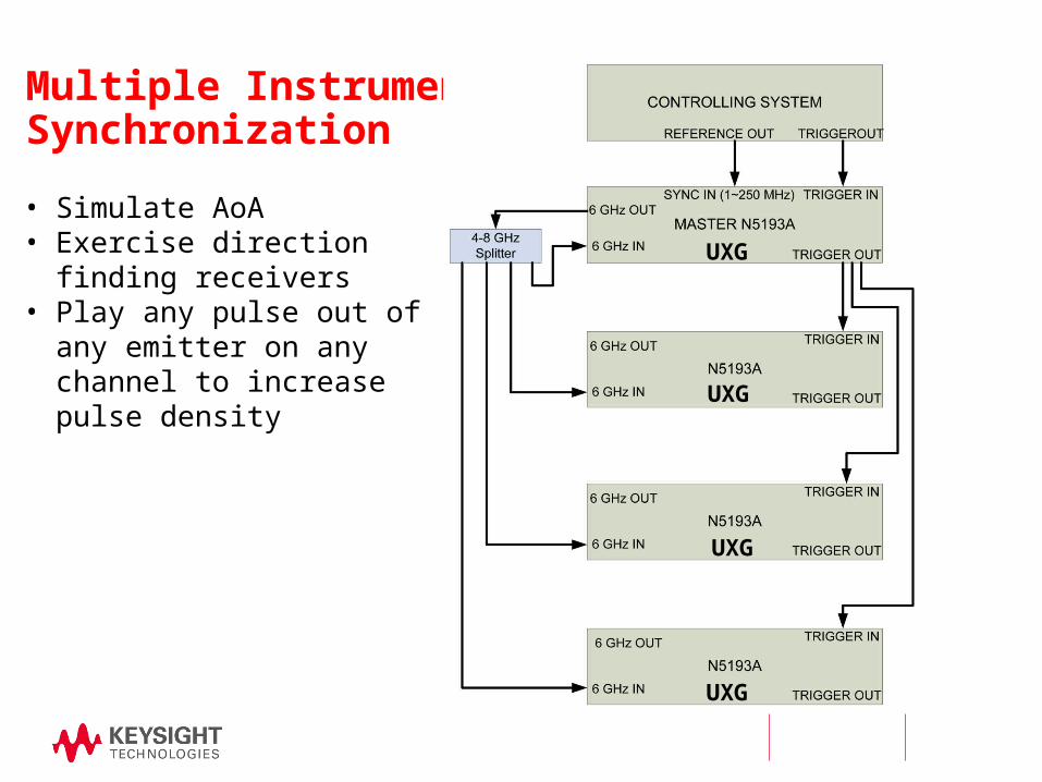
Multiple InstrumentSynchronization

• Simulate AoA• Exercise direction finding

receivers• Play any pulse out of any

emitter on any channel to increase pulse density

UXG

UXG

UXG

UXG

Agenda

• Basic EW• EW test• Multi-emitter simulation• Closed-loop adaptive simulation

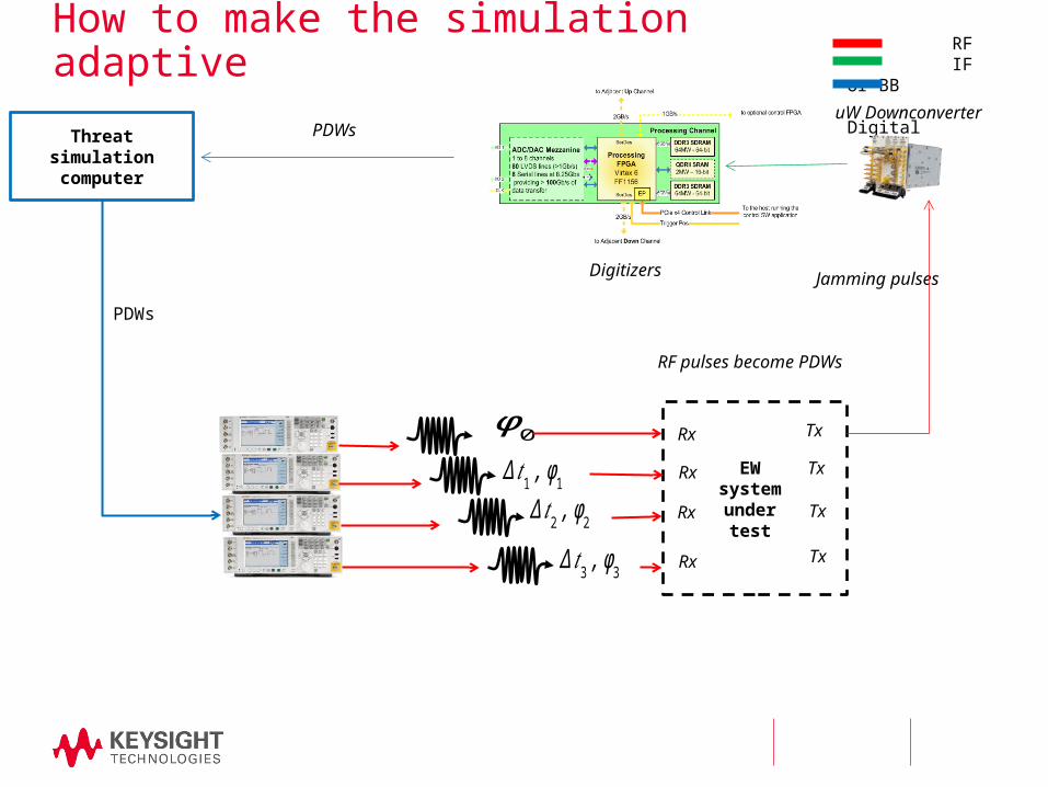
How to make the simulation adaptive

EW system

under test

RF IF or BB Digital

Threat simulation computer

PDWs

φ0∆ 𝑡 1 , φ1∆ 𝑡 2 , φ2∆ 𝑡 3 , φ3

RF pulses become PDWs

Rx Tx

Jamming pulses

Rx

Rx

Rx

Tx

Tx

Tx

PDWs

Digitizers

uW Downconverter

Measurement requirements to enable closed-loop simulation

Signal conditioning: SFDR, noise floor and sensitivity, TOI, low pass filtering for the digitizer

Digitizer: ADC with sufficient sample rate and on-board signal processing resources such as an FPGA to parameterize baseband pulses

Which interface from digitizer?

The PDW-creation architecture – an intermediate solution

RF Pulses uW Signal Conditioning

Local Oscillator Pulse Analysis Software

Simulation computer

(LO for up and downconverters is implied)

Downconverter (Frequency Range:

50 GHzInstantaneous BW:

1GHz)

Digitizers (2) (12 bit 1.6Gbits/sec)

PCI-e Bus

PCI-e Bus

Receiver Hardware Pulse Analysis Software

Gapless Pulse Capture PDW creation and analysis

Real time calculation of Pulse Frequency, Magnitude, Phase

Calculation of PDW Stats

Segmented Memory/Data Decimation

Digital Down Converter

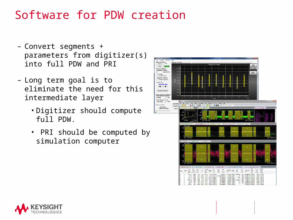
Software for PDW creation

– Convert segments + parameters from digitizer(s) into full PDW and PRI

– Long term goal is to eliminate the need for this intermediate layer

• Digitizer should compute full PDW.

• PRI should be computed by simulation computer

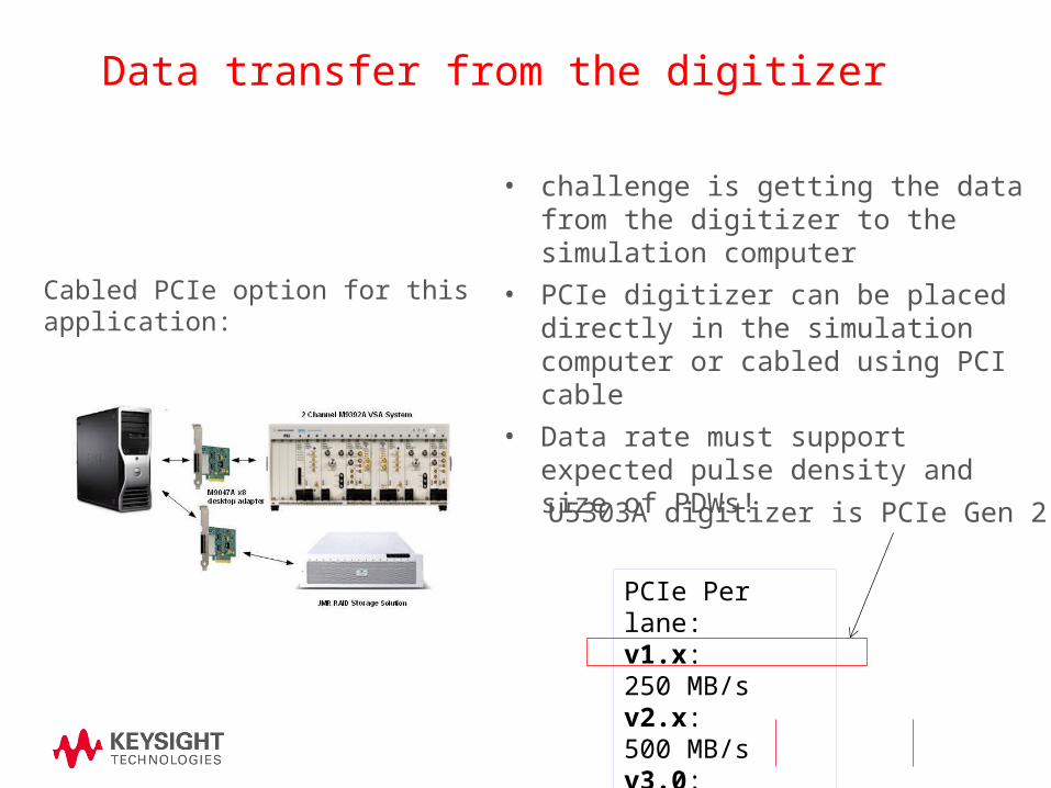
Data transfer from the digitizer

Keysight Confidential

• challenge is getting the data from the digitizer to the simulation computer

• PCIe digitizer can be placed directly in the simulation computer or cabled using PCI cable

• Data rate must support expected pulse density and size of PDWs!

Cabled PCIe option for this application:

PCIe Per lane:v1.x: 250 MB/s v2.x: 500 MB/s v3.0: 985 MB/s

U5303A digitizer is PCIe Gen 2

A final look at our adaptive simulation

EW system

under test

RF IF or BB Digital

Threat simulation computer

PDWs

φ0∆ 𝑡 1 , φ1∆ 𝑡 2 , φ2∆ 𝑡 3 , φ3

RF pulses become PDWs

Rx Tx

Jamming pulses

Rx

Rx

Rx

Tx

Tx

Tx

PDWs

Digitizers

uW Downconverter

Do we have low-enough latency through the analysis chain to meet requirements?

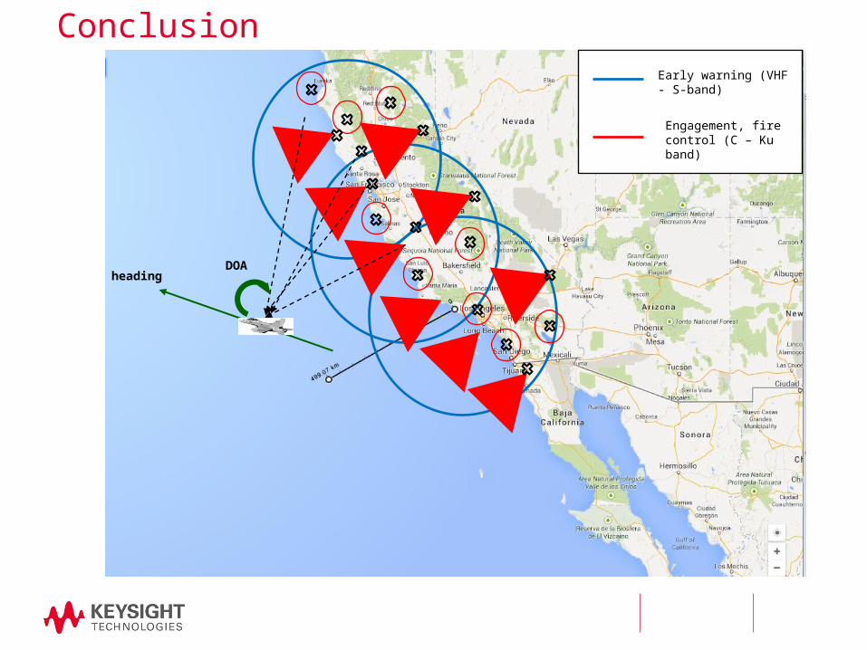
ConclusionEarly warning (VHF - S-band)

Engagement, fire control (C – Ku band)

headingDOA

Resources

– N5193A UXG agile signal generator: www.keysight.com/find/uxg

– N7660B MESG: www.keysight.com/find/N7660B <coming in March!>

– “Electronic warfare signal generation: technologies and methods”

• http://literature.cdn.keysight.com/litweb/pdf/5992-0094EN.pdf