aerosol optical depth analysis with noaa goes and poes … · aerosol optical depth analysis with...
TRANSCRIPT
Calhoun: The NPS Institutional Archive
Theses and Dissertations Thesis Collection
2002-06
Aerosol optical depth analysis with NOAA GOES
and POES in the Western Atlantic
Kuciauskas, Arunas P.
Monterey California. Naval Postgraduate School
http://hdl.handle.net/10945/5886
NAVAL POSTGRADUATE SCHOOL Monterey, California
THESIS
Approved for public release; distribution is unlimited.
AEROSOL OPTICAL DEPTH ANALYSIS WITH NOAA GOES AND POES IN THE WESTERN ATLANTIC
by
Arunas P. Kuciauskas
June 2002
Thesis Advisor: P.A. Durkee Co-Advisor: D.L. Westphal

THIS PAGE INTENTIONALLY LEFT BLANK
i
REPORT DOCUMENTATION PAGE Form Approved OMB No. 0704-0188
Public reporting burden for this collection of information is estimated to average 1 hour per response, including the time for reviewing instruction, searching existing data sources, gathering and maintaining the data needed, and completing and reviewing the collection of information. Send comments regarding this burden estimate or any other aspect of this collection of information, including suggestions for reducing this burden, to Washington headquarters Services, Directorate for Information Operations and Reports, 1215 Jefferson Davis Highway, Suite 1204, Arlington, VA 22202-4302, and to the Office of Management and Budget, Paperwork Reduction Project (0704-0188) Washington DC 20503. 1. AGENCY USE ONLY (Leave blank) 2. REPORT DATE
June 2002 3. REPORT TYPE AND DATES COVERED
Master’s Thesis 4. TITLE AND SUBTITLE Aerosol Optical Depth Analysis with NOAA GOES and POES in the Western Atlantic
5. FUNDING NUMBERS
6. AUTHOR (S) Arunas P. Kuciauskas 7. PERFORMING ORGANIZATION NAME(S) AND ADDRESS(ES) Naval Postgraduate School Monterey, CA 93943-5000
8. PERFORMING ORGANIZATION REPORT NUMBER
9. SPONSORING / MONITORING AGENCY NAME(S) AND ADDRESS(ES) 10. SPONSORING/MONITORING AGENCY REPORT NUMBER
11. SUPPLEMENTARY NOTES The views expressed in this thesis are those of the author and do not reflect the official policy or position of the U.S. Department of Defense or the U.S. Government.
12a. DISTRIBUTION / AVAILABILITY STATEMENT Approved for public release; distribution is unlimited.
12b. DISTRIBUTION CODE
13. ABSTRACT (maximum 200 words)
An aerosol optical depth retrieval algorithm in the visible wavelengths for the NOAA POES AVHRR and GOES -8
visible imager is presented for the cloud free, marine atmosphere. The algorithm combines linearized single-scatter theory
with an estimate of surface reflectance. Phase functions are parameterized using an aerosol size distribution model and the
ratio of radiance values measured in channels 1 and 2 of the AVHRR. Retrieved satellite aerosol optical depth (AOD) is
compared to three land-based sun photometer stations located on islands in the western Atlantic during July and September,
2001. GOES-8 channel 1 (visible wavelength) radiance values were initially calibrated using techniques developed by Rao.
Additional corrections to the channel 1 GOES-8 radiances were made by applying a linear offset factor obtained during the
experimental time period through comparison with AVHRR radiances. The results for the GOES -derived AOD compare
favorably to the AERONET-measured AOD values. For both NOAA and GOES data, the comparison dataset has a
correlation coefficient of 0.67 with a standard error of 0.07. For higher AOD cases (d = 0.25), the general trend was for the
satellite-derived AOD values to underestimate AERONET-observed conditions. During these higher conditions, the
scattering phase function pattern contained within the algorithm deviated from the expected pattern, especially between
140o – 180o. Overall, the more accurate calculations of AOD occurred over scatter angles between 140o - 150o and 170o –
180o.
14. SUBJECT TERMS
Radiative transfer, NOAA AVHRR, POES, GOES, aerosol optical depth, AOD, dust, Caribbean Sea.
15. NUMBER OF PAGES 101
16. PRICE CODE 17. SECURITY CLASSIFICATION OF REPORT
Unclassified
18. SECURITY CLASSIFICATION OF THIS PAGE
Unclassified
19. SECURITY CLASSIFICATION OF ABSTRACT
Unclassified
20. LIMITATION OF ABSTRACT
UL NSN 7540-01-280-5500 Standard Form 298 (Rev. 2-89)
Prescribed by ANSI Std. 239-18

ii
THIS PAGE INTENTIONALLY LEFT BLANK

iii
Approved for public release; distribution is unlimited
AEROSOL OPTICAL DEPTH ANALYSIS WITH NOAA GOES AND POES IN THE WESTERN ATLANTIC
Arunas P. Kuciauskas Civilian, NP-1340 Career Level 3
B.S., The Pennsylvania State University, 1979
Submitted in partial fulfillment of the requirements for the degree of
MASTER OF SCIENCE IN METEOROLOGY
from the
NAVAL POSTGRADUATE SCHOOL June 2002
Author: Arunas P. Kuciauskas
Approved by: Philip A. Durkee, Thesis Advisor
Douglas L. Westphal, Co-Advisor
Carlyle H. Wash, Chairman Department of Meteorology

iv
THIS PAGE INTENTIONALLY LEFT BLANK
v
ABSTRACT
An aerosol optical depth retrieval algorithm in the visible wavelengths for the
NOAA POES AVHRR and GOES-8 visible imager is presented for the cloud free,
marine atmosphere. The algorithm combines linearized single-scatter theory with an
estimate of surface reflectance. Phase functions are parameterized using an aerosol size
distribution model and the ratio of radiance values measured in channels 1 and 2 of the
AVHRR. Retrieved satellite aerosol optical depth (AOD) is compared to three land-
based sun photometer stations located on islands in the western Atlantic during July and
September, 2001. GOES-8 channel 1 (visible wavelength) radiance values were initially
calibrated using techniques developed by Rao. Additional corrections to the channel 1
GOES-8 radiances were made by applying a linear offset factor obtained during the
experimental time period through comparison with AVHRR radiances. The results for
the GOES-derived AOD compare favorably to the AERONET-measured AOD values.
For both NOAA and GOES data, the comparison dataset has a correlation coefficient of
0.67 with a standard error of 0.07. For highe r AOD cases (d = 0.25), the general trend
was for the satellite-derived AOD values to underestimate AERONET-observed
conditions. During these higher conditions, the scattering phase function pattern
contained within the algorithm deviated from the expected pattern, especially between
140o – 180o. Overall, the more accurate calculations of AOD occurred over scatter angles
between 140o - 150o and 170o – 180o.

vi
THIS PAGE INTENTIONALLY LEFT BLANK

vii
TABLE OF CONTENTS
I. INTRODUCTION........................................................................................................1
II. THEORY......................................................................................................................5 A. RADIATIVE TRANSFER THEORY............................................................5 B. OPTICAL DEPTH...........................................................................................6 C. SCATTERING PHASE FUNCTION (p(ψS))................................................8 D. SUMMARY OF ASSUMPTIONS TO THE NPS ALGORITHM ..............9
III. DATA ..........................................................................................................................11 A. INSTRUMENTS ............................................................................................11
1. NOAA Advanced Very High Resolution Radiometer (AVHRR)..11 2. GOES-8 Imager..................................................................................12 3. AERONET Sun-sky Scanning Spectral Radiometer......................12
IV. METHODOLOGY ....................................................................................................15 A. SELECTION OF CASES ..............................................................................15 B. GOES-8 CALIBRATION AND CORRECTION PROCESSES ...............15 C. AOD RETRIEVAL FROM SATELLITE DATA.......................................18
1. Pre-Processing Stage..........................................................................18 2. Processing Stage .................................................................................18
a. Scattering Phase Function Processing ..................................19 3. Post-Processing Stage ........................................................................20
V. RESULTS ...................................................................................................................29 A. CASE 25 SEPTEMBER 2001. LOW AOD CONDITIONS OVER
BERMUDA.....................................................................................................29 1. Synoptic Discussion............................................................................29 2. AOD and Phase Function Analysis ..................................................30
B. CASE 18 SEPTEMBER 2001. HIGH AOD CONDITIONS OVER GUADALOUPE ISLAND.............................................................................31 1. Synoptic Discussion............................................................................31 2. AOD and Phase Function Analysis ..................................................32
C. RESULTS FROM 22 CASES .......................................................................33 1. Evaluation of the NPS Algorithm.....................................................34
VI. CONCLUSIONS AND RECOMMENDATIONS...................................................63 A. CONCLUSIONS ............................................................................................63 B. RECOMMENDATIONS...............................................................................64
APPENDIX A. ........................................................................................................................67
APPENDIX B. ........................................................................................................................69
LIST OF REFERENCES ......................................................................................................81
INITIAL DISTRIBUTION LIST.........................................................................................83

viii
THIS PAGE INTENTIONALLY LEFT BLANK
ix
LIST OF FIGURES Figure 1. Polar plot of scattering phase function describing the scatter angle of
incident radiation with an aerosol particle. ......................................................10 Figure 2. Schematic of solar radiation trajectories that interact once (single scatter)
with aerosol particles and eventually reach the satellite sensor. Path “A” describes direct scatter while paths “B” and “C” indicate diffuse scatter. ......10
Figure 3. Map of the experimental region with locations of the AERONET stations. ...14 Figure 4. Comparisons of radiance images and associated frequency of radiance
histograms between (a) GOES-8 and (b) NOAA-16 on 02 September 2001. Histograms were developed from areas within red annotations. Radiances, as shown within the color legend and the histogram x axis, are in units of Wm-2sr-1µm-1...................................................................................21
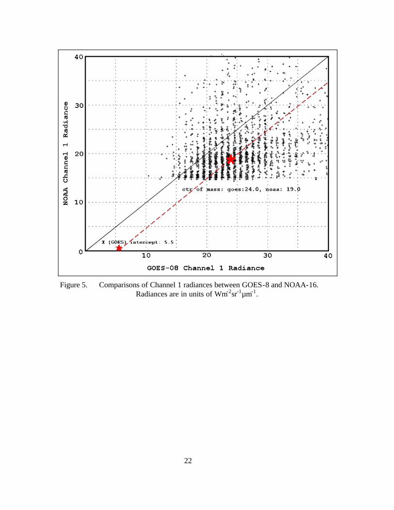
Figure 5. Comparisons of Channel 1 radiances between GOES-8 and NOAA-16. Radiances are in units of Wm-2sr-1µm-1. ..........................................................22
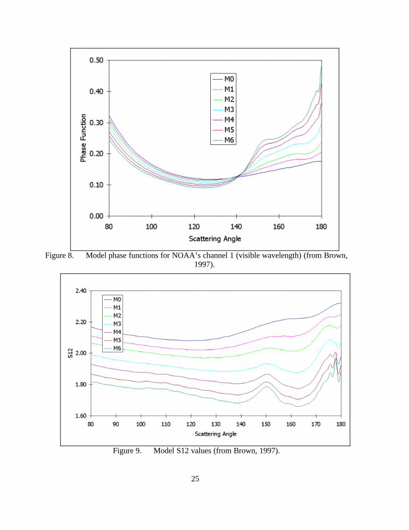
Figure 6. Satellite AOD retrieval process (portions obtained from Brown, 1997). ........23 Figure 7. Model aerosol size distributions (from Brown, 1997). ....................................24 Figure 8. Model phase functions for NOAA’s channel 1 (visible wavelength) (from
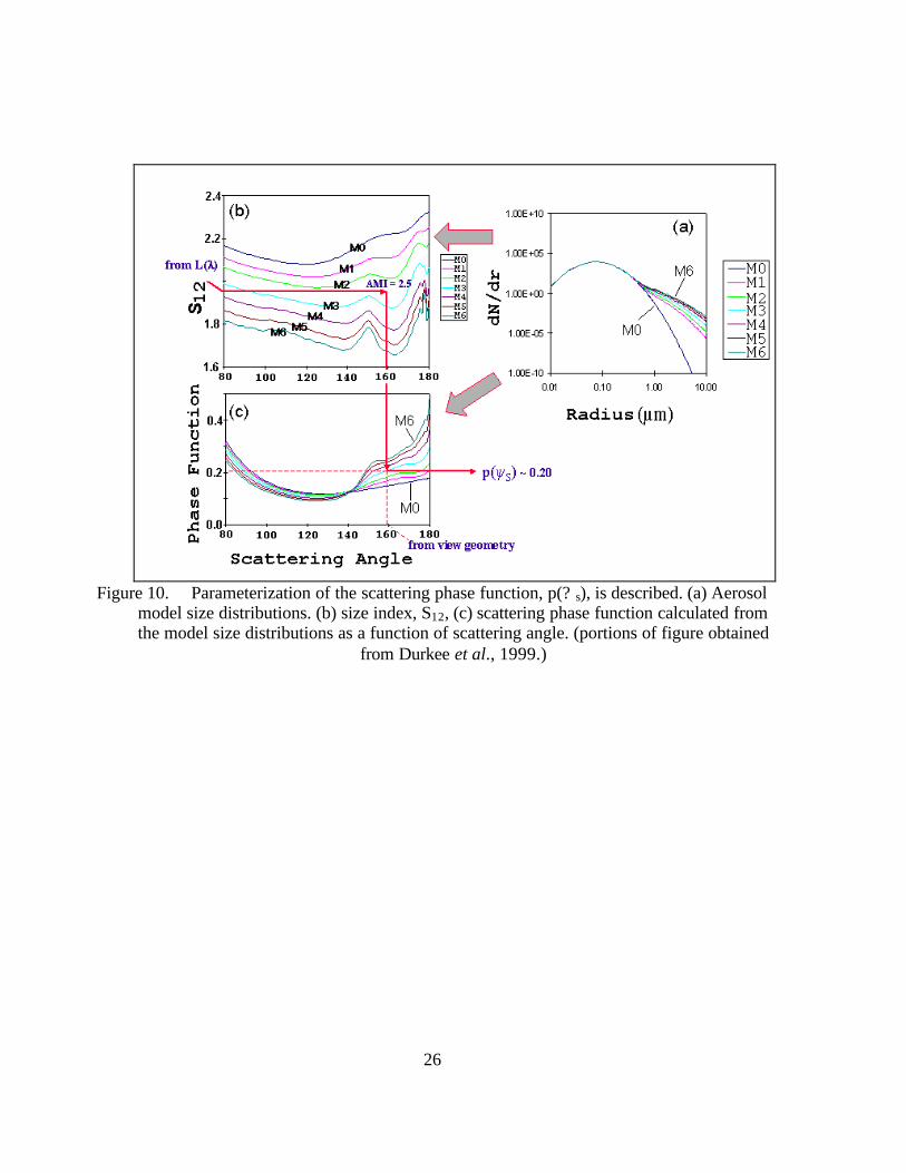
Brown, 1997). ..................................................................................................25 Figure 9. Model S12 values (from Brown, 1997). ..........................................................25 Figure 10. Parameterization of the scattering phase function, p(? s), is described. (a)
Aerosol model size distributions. (b) size index, S12, (c) scattering phase function calculated from the model size distributions as a function of scattering angle. (portions of figure obtained from Durkee et al., 1999.) .......26
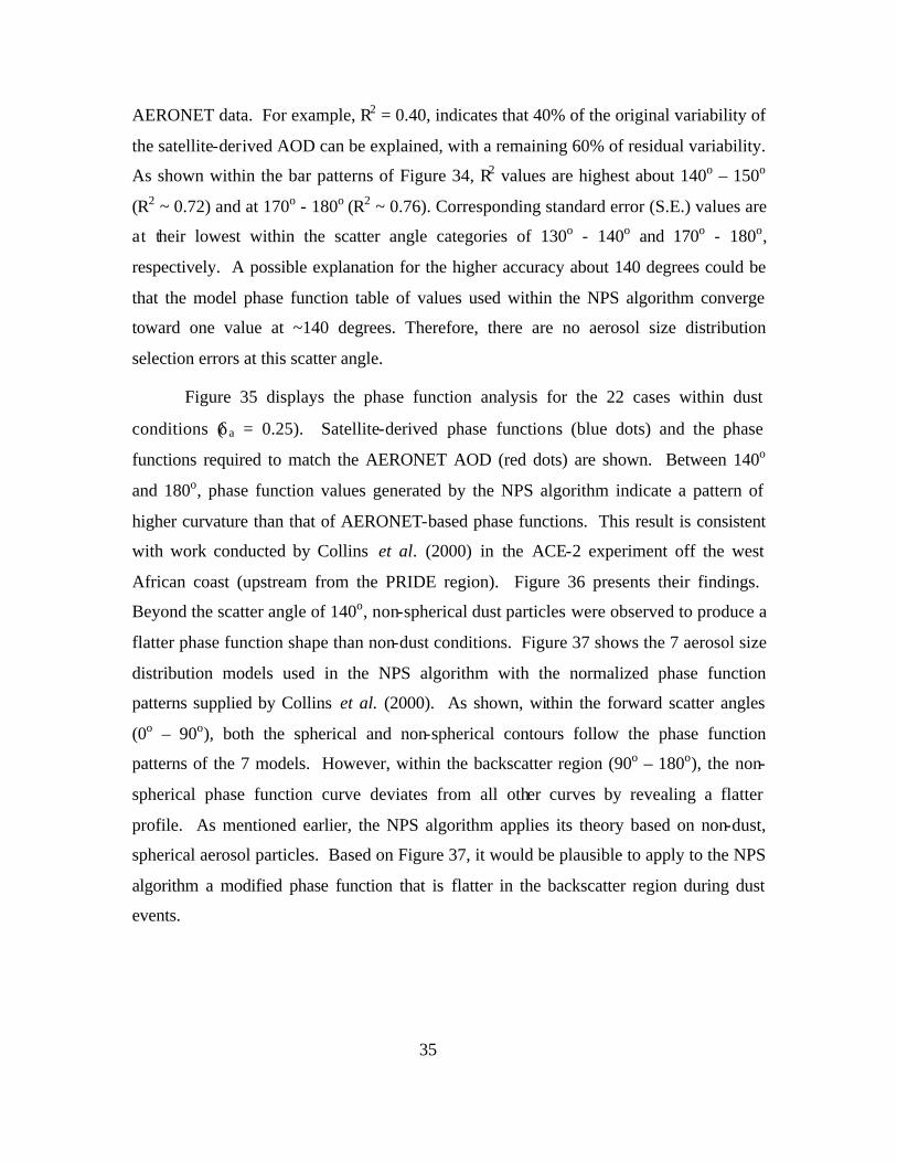
Figure 11. Composite of SeaWiFs images centered at 12 UTC on (a) 24 September, 2001 and (b) 25 September 2001 covering the Atlantic Basin. The location of interest for this study is the island of Bermuda. Over the ocean, clear (low aerosol content) regions are in dark blue, cloudy regions are solid white, and gray regions depict higher aerosol (dust) content. A large plume of dust is visible off of the west coast of Africa. (Courtesy of Dr. Douglas L. Westphal at NRL) ...................................................................36
Figure 12. Plot of NAAPS display of optical depth for sulfate (red shades), dust and smoke (green and yellow shades) over the Atlantic Ocean basin for 25 September 2001, 18:00 UTC. The bottom color bar shows the AOD range for dust and smoke. 850 mb model-generated wind barbs are also displayed. (Courtesy of Dr. Douglas L. Westphal at NRL) .............................37
Figure 13. GOES-8 visible image on 25 September 2001 at 17:15 UTC. The annotated box surrounds the region of Bermuda. ............................................38
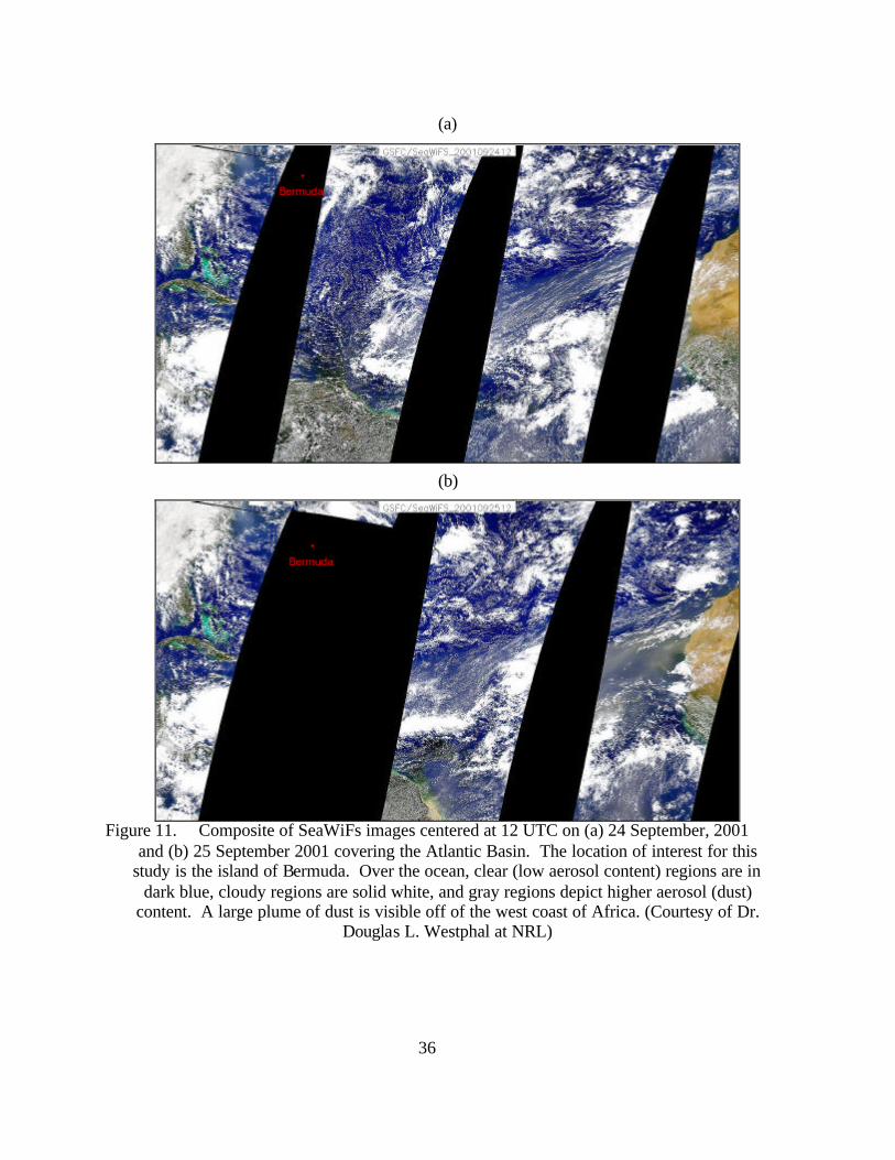
Figure 14. Time series of AOD images generated for 25 September 2001 from GOES-8 data that surrounds Bermuda. Pixel sizes are 1.1 km by 1.1 km and the domain is approximately 110 km by 110 km. The times range from 13:15 UTC to 16:15 UTC. Red boxes depict locations where the
x
representative AOD for that area was measured. AOD color contours are defined on the left side of each image..............................................................39
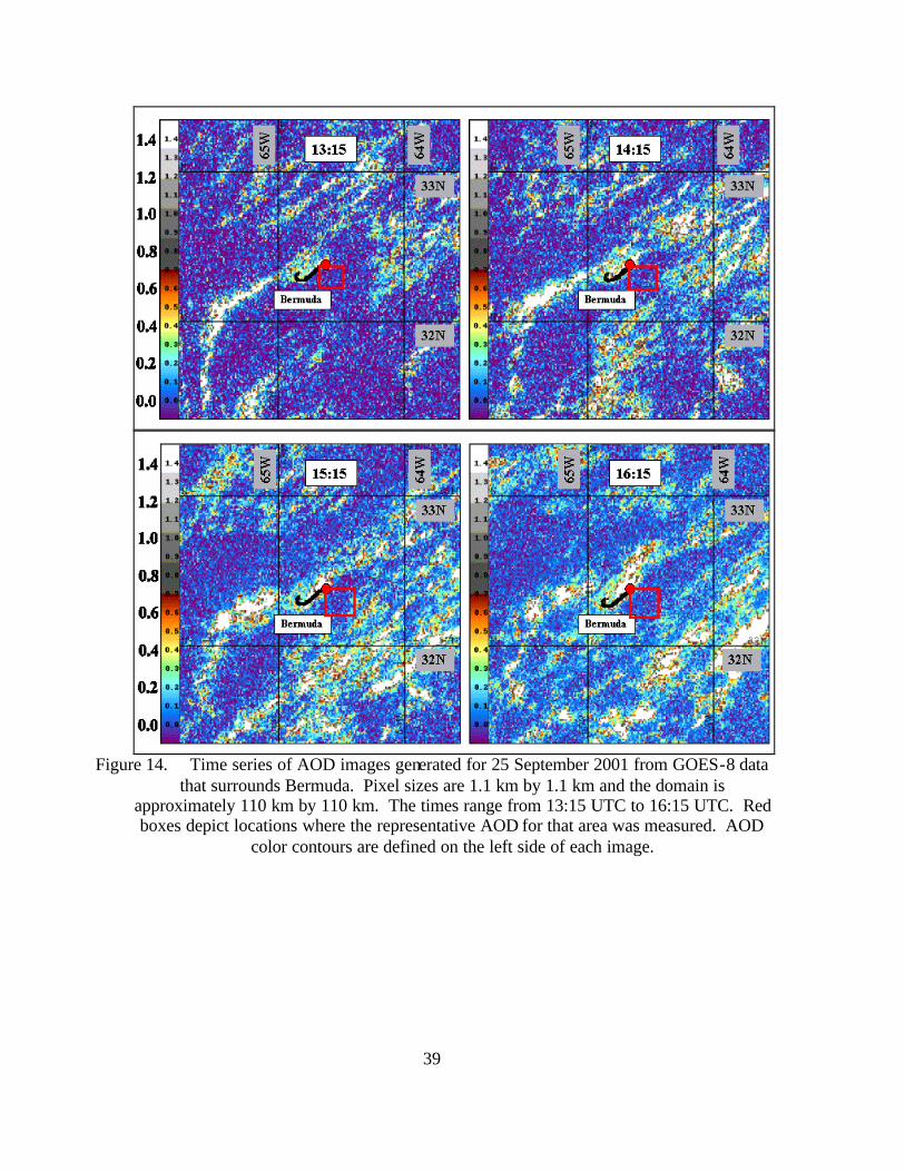
Figure 15. Continuation of Figure 14 for times ranging from 17:15 UTC to 20:15 UTC..................................................................................................................40
Figure 16. AOD image generated for 25 September 2001 at 18:17 UTC from NOAA-16 data that surrounds Bermuda. Pixel sizes are 1.1 km by 1.1 km and the domain is approximately 110 km by 110 km. Red box depicts the location where the representative AOD for that area was measured. AOD color contours are defined on the left side of the image. ..........................................41
Figure 17. An example of a his togram frequency plot for determining AOD. A normalized curve (solid red curve) displays the distribution, where the center of mass (*) is situated at the top of the curve. The resulting AOD value of 0.03 is then obtained. The variability measurements of AOD are obtained from a line drawn at half the amplitude of the normalized curve that indicates one standard deviation from the measured AOD value. ............42
Figure 18. Time series of histogram plots of AOD for 25 September 2001, between 13:15 UTC and 16:45 UTC. Plots are generated from boxes defined in Figure 14. The AOD values are shown in red, while the two adjacent values represent the variability of AOD measurements. The red annotations depict the AOD measurement process that is described in Figure 17. .........................................................................................................43
Figure 19. Continuation of time series of histogram plots from Figure 15 of AOD for 25 September 2001, between 17:15 UTC and 20:15 UTC. .............................44
Figure 20. Histogram plot of AOD for 25 September 2001 at 18:17 UTC from NOAA-16 data. The plot is generated from box defined in Figure 16. Times are in UTC. The AOD values are shown in red, while the two adjacent values represent the variability in the AOD measurement. ...............45
Figure 21. Time series of AOD for both satellite-derived data (navy blue dots) and AERONET observations (yellow) for 25 September 2001 over Bermuda. NOAA data are presented as individual blue dots whereas GOES-8 data are connected with a blue line. Red bars represent variability in AOD measurements. The corresponding scatter angle profile is represented as a purple dashed line. ...........................................................................................46
Figure 22. Plot of phase function as a function of scatter angle for the case of 25 September 2001 over Bermuda. Blue diamonds indicate phase functions obtained from satellite data. Red boxes indicate phase function values required for the satellite-derived AOD to match AERONET’s AOD. ............47
Figure 23. Composite of SeaWiFs images centered at 12 UTC on (a) 17 September 2001 and (b) 18 September, 2001 covering the Atlantic Basin. The location of interest for this study is Guadaloupe Island. Over the ocean, clear (low aerosol content) regions are in dark blue, cloudy regions are solid white, and gray regions depict higher aerosol (dust) content. A large plume of dust is visible off of the west coast of Africa. (Courtesy of Dr. Douglas L. Westphal at NRL)..........................................................................48
xi
Figure 24. Plot of NAAPS display of optical depth for sulfate (red shades), dust and smoke (green and yellow shades) over the Atlantic Ocean basin for 18 September 2001, 18:00 UTC. (Courtesy of Dr. Douglas L. Westphal at NRL) ................................................................................................................49
Figure 25. GOES-8 visible image on 18 September 2000 at 17:15 UTC. The annotated box surrounds the region of Guadaloupe Island. The area of aerosol dust is also annotted. ...........................................................................50
Figure 26. Time series of AOD images generated for 18 September 2001 from GOES-8 data that surrounds Guadaloupe Island. Pixel sizes are 1.1 km by 1.1 km and the domain is approximately 110 km by 110 km. The times range from 16:45 UTC to 18:15 UTC. Red boxes depict locations where the representative AOD for that area was measured. AOD color contours are defined on the left side of each image........................................................51
Figure 27. Continuation of Figure 26 for times ranging from 19:15 UTC to 20:45 UTC..................................................................................................................52
Figure 28. AOD images generated for 18 September 2001 at 17:50 UTC and 21:16 UTC from NOAA-16 and NOAA-14 data, respectively. Images surround Guadaloupe Island. Pixel sizes are 1.1 km by 1.1 km and the domain is approximately 110 km by 110 km. Red boxes depict the locations where the representative AOD for that area were measured. AOD color contours are defined on the left side of each image........................................................53
Figure 29. Time series of frequency histogram plots of AOD for 18 September 2001, between 16:45 UTC and 21:16 UTC. The top 6 plots are derived from GOES-8 data and the bottom 2 plots are derived from NOAA-16 and NOAA-14 data, respectively. Plots are generated from boxes defined in Figures 26 and 27. For each plot, the AOD value is shown in red, while the pair of black values represent the variability of AOD measurements. The red lines and curves depict the AOD measurement process that is described in Figure 17......................................................................................54
Figure 30. Chart of AOD for both satellite-derived data (navy blue dots) and AERONET observations (yellow) for 18 September 2001 over Guadaloupe Island. NOAA data are presented as individual blue dots whereas GOES-8 data are connected with a blue line. Red bars represent variability in AOD measurements. The corresponding scatter angle profile is represented as a purple dashed line. .............................................................55
Figure 31. Plot of phase function as a function of scatter angle for the case of 18 September 2001 over Guadaloupe Island. Blue diamonds indicate phase functions obtained from satellite data. Red boxes indicate the phase function values required for the satellite-derived AOD to match AERONET AOD. ............................................................................................56
Figure 32. Distribution of distance measurements between each of the 3 AERONET sites and the location of the satellite-derived AOD for all 22 cases. For each AERONET region, the average distance from the AERONET station to the center of the satellite-derived measurement box is annotated in red. ....57
xii
Figure 33. Comparisons between NPS-calculated AOD and AERONET-observations of AOD for the 22 cases as listed in Appendix A.1. The red line depicts one to one relationship. ....................................................................................58
Figure 34. Evaluation of NPS algorithm, partitioned over categories of scatter angles. ..59 Figure 35. Comparisons of phase functions between satellite data and AERONET
data for 22 cases. Figure only depicts dust conditions (AERONET AOD = 0.25)..............................................................................................................60
Figure 36. Phase function plots for the free troposphere, dust layer obtained from the second Aerosol Characterization Experiment (ACE-2). Data is supplied by Collins, et al. (2000). Phase function values are normalized.....................60
Figure 37. Phase function plots comparing the dust plots in Collins et al. (2000) (thick curves) with the model phase functions used in the NPS algorithm (thin curves). Annotated numbers are used to identify the model numbers. ..61

xiii
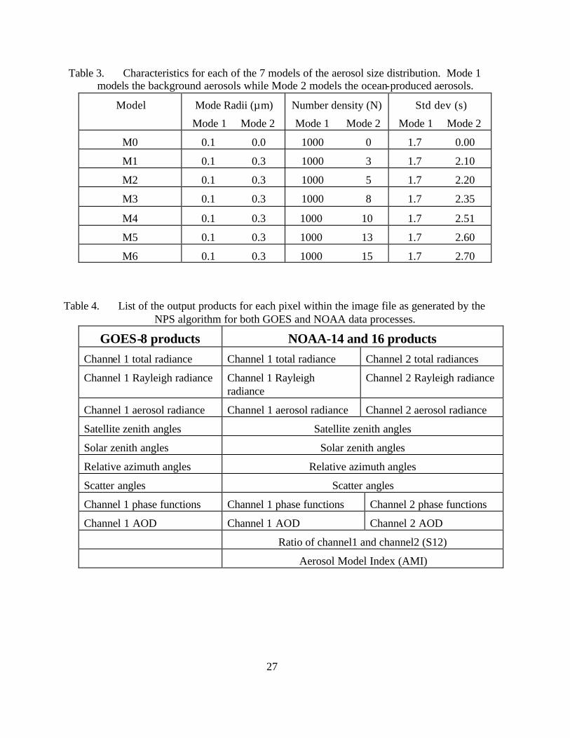
LIST OF TABLES Table 1. NOAA AVHRR Radiometric Channels. .........................................................13 Table 2. GOES Imager Radiometric Channels ..............................................................13 Table 3. Characteristics for each of the 7 models of the aerosol size distribution.
Mode 1 models the background aerosols while Mode 2 models the ocean-produced aerosols.............................................................................................27
Table 4. List of the output products for each pixel within the image file as generated by the NPS algorithm for both GOES and NOAA data processes. .........................................................................................................27
Table 5. List of 22 cases that include the GOES and NOAA pass times (in UTC) and locations. The case studies are identified in sequential numbers, shown in parentheses. ......................................................................................67

xiv
THIS PAGE INTENTIONALLY LEFT BLANK

xv
ACKNOWLEDGEMENTS
I wish to thank Dr. Douglas Myhre of University of South Florida as well as Dr.
Fernando Gilbes of University of Puerto Rico for their prompt and helpful responses to
my requests of NOAA satellite data. In addition, I would like to express my appreciation
to the NOAA NESDIS satellite personnel for having developed an efficient NOAA
AVHRR satellite data acquisition web site. I would also like to thank Dr. Joe Turk at the
Naval Research Laboratory (NRL) for establishing daily GOES-8 image data. I would
like to thank Mr. Brent Holben and Ms. Rose Petit from AERONET for providing me
with sun photometer data. To Mr. Kim Richardson of NRL and Mr. Robert Wade of
SAIC, thanks for your constructive criticisms during my data analysis time period.
Thanks also to Dr. Westphal, my second thesis reader, for providing me with your vast
experience as well as a realistic picture of the difficulties of assessing global visibility
over the world’s open waters. I am greatly indebted to Mr. Jeff Hawkins, my department
head, as well as the Administrative staff at NRL, for allowing me to devote 40% of my
work time to school and thesis work. I am greatly indebted to Dr. Phil Durkee who
initially stimulated my interest in the field of remote sensing of the atmosphere and
provided me with continuous guidance throughout my thesis endeavor. Finally, to my
wife Stacey; you were a great motivator and very patient with all of the long hours I spent
away from you.

xvi
THIS PAGE INTENTIONALLY LEFT BLANK

1
I. INTRODUCTION
Monitoring tropospheric aerosols on a global scale is essential for evaluating the
earth’s radiation budget. Aerosols are known to cause a net cooling effect by scattering
incident solar radiation back to space and by interacting with clouds in a way that
increases overall albedo (Charlson et al., 1992, Twomey et al., 1977, IPCC, 1996). King
et al. (1999) reports that the impact of aersosol radiative forcing, both directly
(scattering) and indirectly (interaction with clouds), produces a cooling range of
–1.4±1.5 W m-2 to –2.5±2 W m-2. This result offsets the well-known concept of the
greenhouse warming impact, estimated to be +2.5±0.3 W m-2.
Assessing aerosol properties also has military implications. Infrared wavelength
image and ranging systems, laser-guided weapons systems, and laser communication
systems are sensitive to the environment. Infrared imaging and ranging systems are
strongly affected by variations of atmospheric aerosols. Laser systems used for radio and
satellite communications operate within the visible and near-IR wavelength ranges, and
can be greatly affected by varying aerosol properties, such as density, size distribution,
chemical and physical composition (Bloembergen et al. 1987; Cordray et al. 1977).
Brown (1997) reports that the proper interpretation of aerosol radiative properties in the
coastal zone is “important to the design, planning, and operation of electro-optical
weapons and sensor systems near coastal boundaries”.
Another research area of global aerosol impact focuses on the transport of dust and
pollutants from one region to another. ACE-Asia is a 4-year project (2001 – 2004)
devoted to the study of aerosol profiles in the Pacific basin generated by desert dust and
industrial pollution over Asia. The Puerto Rico Dust Experiment (PRIDE) in 2000
studied the impacts of African desert dust that is transported over to the Caribbean and
the eastern U.S.
Given the challenges listed above, there is a developing interest to globally quantify
aerosol properties on fine spatial and temporal scales. Thus far, this analysis has proven
to be a daunting task, since most established aerosol sensing is land-based, providing
2
poor spatial and temporal coverage. Higurashi et al. (1999) suggests that aerosol
concentration, size distribution, composition, and optical properties will have to be
measured globally, and that satellite remote sensing is an effective tool for such a task.
Over the past few decades, scientists have developed algorithms to convert satellite
upwelling radiances into aerosol properties such as optical depth. So far, most of the
aerosol remote sensing studies have used the NOAA Advanced Very High Resolution
Radiometer (AVHRR) channel 1 and 2 sensors. These algorithms were developed by
assuming certain aerosol characteristics before processing the upwelling radiances
(Durkee et al. (1991), Kaufman et al. (1990), Higurashi and Nakajima (1999)).
This study focuses on one such algorithm developed by Durkee et al. (1992)
(hereafter referred to as the NPS algorithm). The NPS algorithm ingests AVHRR data
within a cloud-free, single scatter environment. By using the ratio of channel 1 and 2
radiances, an estimate of the aerosol size distribution is extracted. During three recent
field campaigns, Durkee et al. (1999) has shown that the NPS algorithm performs well
for aerosol optical depth (AOD) below about 0.4 at 0.63µm wavelength. But the results
only provided snapshots of the experimental regions, since AVHRR passes over a
particular region a few times per day. Brown (1997) incorporated both the AVHRR and
the Geosynchronous Operational Environmental Satellite (GOES) satellite to provide
temporal coverage of AOD over an experimental region. In the upgraded NPS algorithm,
an aerosol model index is derived from the AVHRR data is applied to the GOES
retrieval. The results were encouraging, but limited. The focus of this report is to expand
this approach. The following issues will be addressed:
• Proper radiance calibration of the visible sensor of GOES
• Validation of the AOD derived from NOAA and GOES-8
• Evaluation of the phase function parameters used in the retrieval algorithm
Chapter II describes the radiative transfer theory and the simplifying atmospheric
assumptions used in the satellite optical depth retrievals. Chapter III describes the data
sets and the instrumentation used. Chapter IV describes the calibration and correction
techniques applied to the retrieved GOES channel 1 radiance. In addition, the AOD
retrieval procedures for both the AVHRR and GOES are discussed. Chapter V discusses

3
the results and Chapter VI presents the conclusions and recommendations for future
research.

4
THIS PAGE INTENTIONALLY LEFT BLANK
5
II. THEORY
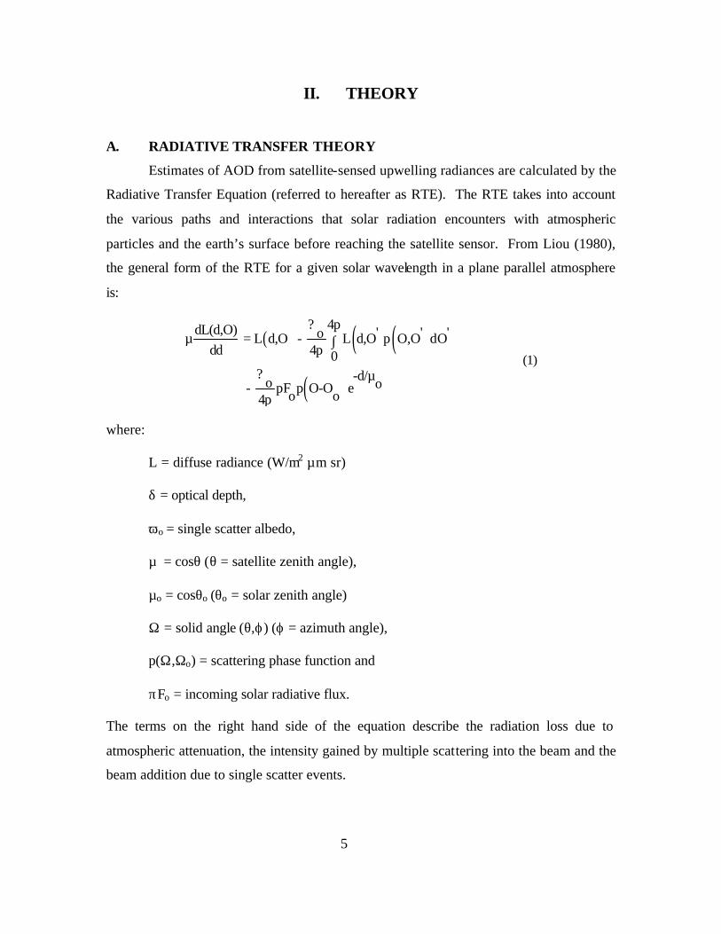
A. RADIATIVE TRANSFER THEORY
Estimates of AOD from satellite-sensed upwelling radiances are calculated by the
Radiative Transfer Equation (referred to hereafter as RTE). The RTE takes into account
the various paths and interactions that solar radiation encounters with atmospheric
particles and the earth’s surface before reaching the satellite sensor. From Liou (1980),
the general form of the RTE for a given solar wavelength in a plane parallel atmosphere
is:
( ) ( ) ( )( )
4p?dL(d,O) ' ' 'oµ = L d,O - L d,O p O,O dOdd 4p 0
? -d/µo o- pF p O-O eo o4p
∫ (1)
where:
L = diffuse radiance (W/m2 µm sr)
δ = optical depth,
ωo = single scatter albedo,
µ = cosθ (θ = satellite zenith angle),
µo = cosθo (θo = solar zenith angle)
Ω = solid angle (θ,ϕ) (ϕ = azimuth angle),
p(Ω,Ωo) = scattering phase function and
πFo = incoming solar radiative flux.
The terms on the right hand side of the equation describe the radiation loss due to
atmospheric attenuation, the intensity gained by multiple scattering into the beam and the
beam addition due to single scatter events.
6
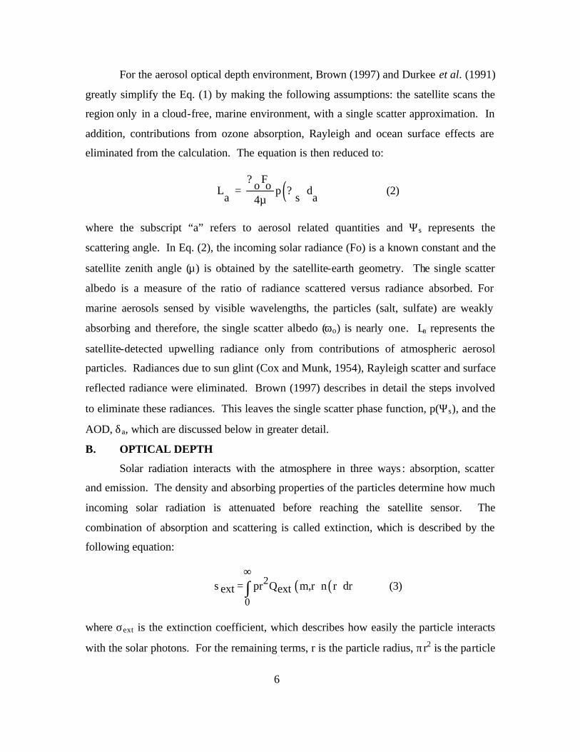
For the aerosol optical depth environment, Brown (1997) and Durkee et al. (1991)
greatly simplify the Eq. (1) by making the following assumptions: the satellite scans the
region only in a cloud-free, marine environment, with a single scatter approximation. In
addition, contributions from ozone absorption, Rayleigh and ocean surface effects are
eliminated from the calculation. The equation is then reduced to:
( )? Fo oL = p ? da s a4µ
(2)
where the subscript “a” refers to aerosol related quantities and Ψs represents the
scattering angle. In Eq. (2), the incoming solar radiance (Fo) is a known constant and the
satellite zenith angle (µ) is obtained by the satellite-earth geometry. The single scatter
albedo is a measure of the ratio of radiance scattered versus radiance absorbed. For
marine aerosols sensed by visible wavelengths, the particles (salt, sulfate) are weakly
absorbing and therefore, the single scatter albedo (ωo) is nearly one. La represents the
satellite-detected upwelling radiance only from contributions of atmospheric aerosol
particles. Radiances due to sun glint (Cox and Munk, 1954), Rayleigh scatter and surface
reflected radiance were eliminated. Brown (1997) describes in detail the steps involved
to eliminate these radiances. This leaves the single scatter phase function, p(Ψs), and the
AOD, δa, which are discussed below in greater detail.
B. OPTICAL DEPTH
Solar radiation interacts with the atmosphere in three ways : absorption, scatter
and emission. The density and absorbing properties of the particles determine how much
incoming solar radiation is attenuated before reaching the satellite sensor. The
combination of absorption and scattering is called extinction, which is described by the
following equation:
( ) ( )2
0
s = pr Q m,r n r drext ext∞
∫ (3)
where σext is the extinction coefficient, which describes how easily the particle interacts
with the solar photons. For the remaining terms, r is the particle radius, πr2 is the particle
7
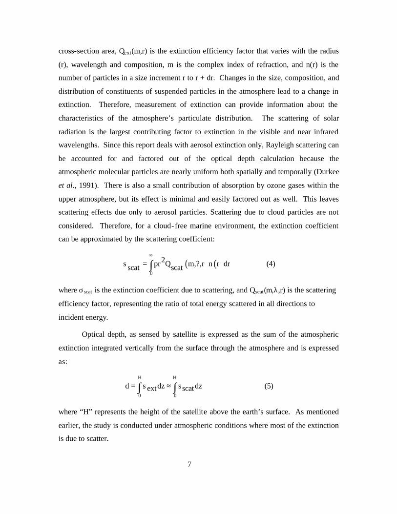
cross-section area, Qext(m,r) is the extinction efficiency factor that varies with the radius
(r), wavelength and composition, m is the complex index of refraction, and n(r) is the
number of particles in a size increment r to r + dr. Changes in the size, composition, and
distribution of constituents of suspended particles in the atmosphere lead to a change in
extinction. Therefore, measurement of extinction can provide information about the
characteristics of the atmosphere’s particulate distribution. The scattering of solar
radiation is the largest contributing factor to extinction in the visible and near infrared
wavelengths. Since this report deals with aerosol extinction only, Rayleigh scattering can
be accounted for and factored out of the optical depth calculation because the
atmospheric molecular particles are nearly uniform both spatially and temporally (Durkee
et al., 1991). There is also a small contribution of absorption by ozone gases within the
upper atmosphere, but its effect is minimal and easily factored out as well. This leaves
scattering effects due only to aerosol particles. Scattering due to cloud particles are not
considered. Therefore, for a cloud-free marine environment, the extinction coefficient
can be approximated by the scattering coefficient:
( ) ( )0
2s pr Q m,?,r n r drscat scat
∞
= ∫ (4)
where σscat is the extinction coefficient due to scattering, and Qscat(m,λ,r) is the scattering
efficiency factor, representing the ratio of total energy scattered in all directions to
incident energy.
Optical depth, as sensed by satellite is expressed as the sum of the atmospheric
extinction integrated vertically from the surface through the atmosphere and is expressed
as:
H H
0 0
d = s dz s dzext scat≈∫ ∫ (5)
where “H” represents the height of the satellite above the earth’s surface. As mentioned
earlier, the study is conducted under atmospheric conditions where most of the extinction
is due to scatter.
8
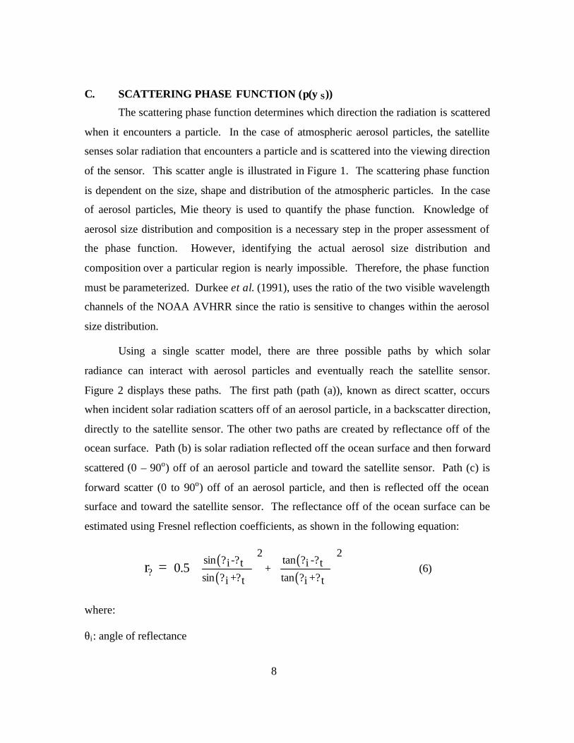
C. SCATTERING PHASE FUNCTION (p(ψS))
The scattering phase function determines which direction the radiation is scattered
when it encounters a particle. In the case of atmospheric aerosol particles, the satellite
senses solar radiation that encounters a particle and is scattered into the viewing direction
of the sensor. This scatter angle is illustrated in Figure 1. The scattering phase function
is dependent on the size, shape and distribution of the atmospheric particles. In the case
of aerosol particles, Mie theory is used to quantify the phase function. Knowledge of
aerosol size distribution and composition is a necessary step in the proper assessment of
the phase function. However, identifying the actual aerosol size distribution and
composition over a particular region is nearly impossible. Therefore, the phase function
must be parameterized. Durkee et al. (1991), uses the ratio of the two visible wavelength
channels of the NOAA AVHRR since the ratio is sensitive to changes within the aerosol
size distribution.
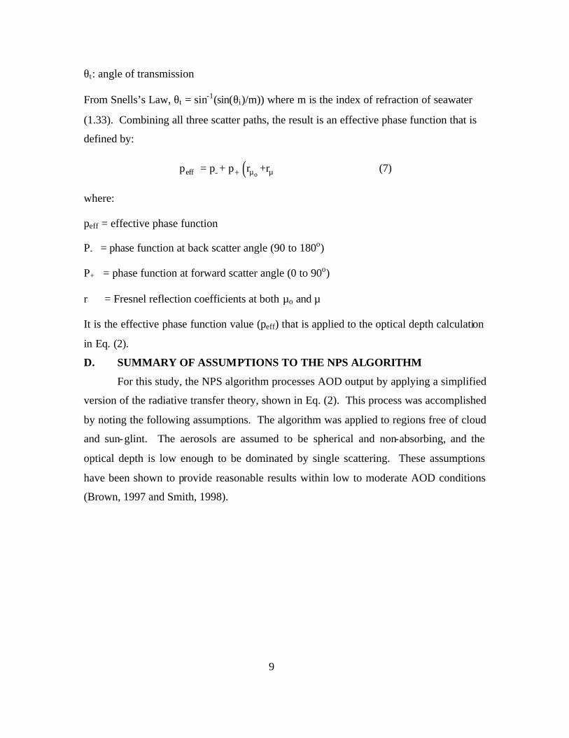
Using a single scatter model, there are three possible paths by which solar
radiance can interact with aerosol particles and eventually reach the satellite sensor.
Figure 2 displays these paths. The first path (path (a)), known as direct scatter, occurs
when incident solar radiation scatters off of an aerosol particle, in a backscatter direction,
directly to the satellite sensor. The other two paths are created by reflectance off of the
ocean surface. Path (b) is solar radiation reflected off the ocean surface and then forward
scattered (0 – 90o) off of an aerosol particle and toward the satellite sensor. Path (c) is
forward scatter (0 to 90o) off of an aerosol particle, and then is reflected off the ocean
surface and toward the satellite sensor. The reflectance off of the ocean surface can be
estimated using Fresnel reflection coefficients, as shown in the following equation:
( )( )
( )( )?
2 2sin ? -? tan ? -?i t i t+ sin ? +? tan ? +?i t i t
0.5r =
(6)
where:
θi: angle of reflectance
9
θt: angle of transmission
From Snells’s Law, θt = sin-1(sin(θi)/m)) where m is the index of refraction of seawater
(1.33). Combining all three scatter paths, the result is an effective phase function that is
defined by:
( )oeff µ µ- +p = p + p r +r (7)
where:
peff = effective phase function
P- = phase function at back scatter angle (90 to 180o)
P+ = phase function at forward scatter angle (0 to 90o)
r = Fresnel reflection coefficients at both µo and µ
It is the effective phase function value (peff) that is applied to the optical depth calculation
in Eq. (2).
D. SUMMARY OF ASSUMPTIONS TO THE NPS ALGORITHM
For this study, the NPS algorithm processes AOD output by applying a simplified
version of the radiative transfer theory, shown in Eq. (2). This process was accomplished
by noting the following assumptions. The algorithm was applied to regions free of cloud
and sun-glint. The aerosols are assumed to be spherical and non-absorbing, and the
optical depth is low enough to be dominated by single scattering. These assumptions
have been shown to provide reasonable results within low to moderate AOD conditions
(Brown, 1997 and Smith, 1998).
10
Figure 1. Polar plot of scattering phase function describing the scatter angle of incident
radiation with an aerosol particle.
Figure 2. Schematic of solar radiation trajectories that interact once (single scatter) with
aerosol particles and eventually reach the satellite sensor. Path “A” describes direct scatter while paths “B” and “C” indicate diffuse scatter.
11
III. DATA
To validate the optical depth retrieval method, case study days were chosen based
on the availability of matching datasets between GOES, NOAA and AERONET. This
chapter briefly describes the data sets and instrumentation used for this study.
A. INSTRUMENTS
1. NOAA Advanced Very High Resolution Radiometer (AVHRR)
The AVHRR instrument senses upwelling radiances of 5 channels, ranging from
visible to infrared. Table 1 describes the bandwidths of these channels. The AVHRR
instrument is part of the National Oceanic and Atmospheric Administration (NOAA)
Polar Orbiting Operational Environmental Satellite (POES) series of satellites. These
satellites are in sun synchronous orbit at a height of 883 km and provide at least four
passes per day over a given region of the earth. The AVHRR scans at nadir with a width
of approximately 2000 km and a sub-satellite pixel resolution of 1.1 km by 1.1 km.
The AVHRR instruments onboard the NOAA-14 (launched on 01 January 1995)
and NOAA-16 (launched on 02 February 2001) satellites provided the data for this study.
Over the experimental region, the NOAA-16 AVHRR provided the local afternoon data
while the NOAA-14 AVHRR provided data late in the afternoon. The data from the
NOAA-14 was at times questionable due to low sun angle problems. Therefore, the
NOAA-16 data was the more reliable dataset.
The AVHRR dataset was transmitted to the receiver at Wallops Island, Virginia,
and archived by the NOAA National Environmental Satellite, Data and Information
Service (NESDIS) Satellite Active Archive, in Level 1b format. AVHRR Level 1b data
is in 10 bit precision format that have been quality controlled, assembled into discrete
data sets, and to which earth location and calibration information has been appended, but
not applied to the data. Other parameters included are time, quality flags, solar zenith
angles, and telemetry. All AVHRR channels are calibrated prior to launch. Channels 1
and 2 have no onboard calibration systems. Post calibration methods for these channels
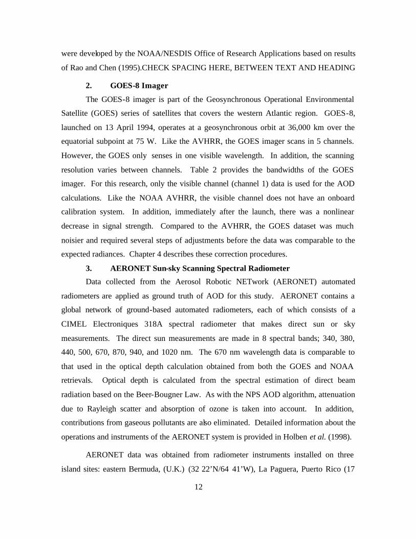
12
were developed by the NOAA/NESDIS Office of Research Applications based on results
of Rao and Chen (1995).CHECK SPACING HERE, BETWEEN TEXT AND HEADING
2. GOES-8 Imager
The GOES-8 imager is part of the Geosynchronous Operational Environmental
Satellite (GOES) series of satellites that covers the western Atlantic region. GOES-8,
launched on 13 April 1994, operates at a geosynchronous orbit at 36,000 km over the
equatorial subpoint at 75 W. Like the AVHRR, the GOES imager scans in 5 channels.
However, the GOES only senses in one visible wavelength. In addition, the scanning
resolution varies between channels. Table 2 provides the bandwidths of the GOES
imager. For this research, only the visible channel (channel 1) data is used for the AOD
calculations. Like the NOAA AVHRR, the visible channel does not have an onboard
calibration system. In addition, immediately after the launch, there was a nonlinear
decrease in signal strength. Compared to the AVHRR, the GOES dataset was much
noisier and required several steps of adjustments before the data was comparable to the
expected radiances. Chapter 4 describes these correction procedures.
3. AERONET Sun-sky Scanning Spectral Radiometer
Data collected from the Aerosol Robotic NETwork (AERONET) automated
radiometers are applied as ground truth of AOD for this study. AERONET contains a
global network of ground-based automated radiometers, each of which consists of a
CIMEL Electroniques 318A spectral radiometer that makes direct sun or sky
measurements. The direct sun measurements are made in 8 spectral bands; 340, 380,
440, 500, 670, 870, 940, and 1020 nm. The 670 nm wavelength data is comparable to
that used in the optical depth calculation obtained from both the GOES and NOAA
retrievals. Optical depth is calculated from the spectral estimation of direct beam
radiation based on the Beer-Bougner Law. As with the NPS AOD algorithm, attenuation
due to Rayleigh scatter and absorption of ozone is taken into account. In addition,
contributions from gaseous pollutants are also eliminated. Detailed information about the
operations and instruments of the AERONET system is provided in Holben et al. (1998).
AERONET data was obtained from radiometer instruments installed on three
island sites: eastern Bermuda, (U.K.) (32 22’N/64 41’W), La Paguera, Puerto Rico (17
13
58’N/67 02’W) and Guadaloup, Island (Fr.) (16 19’N/61 30’W), all within the western
Atlantic Basin (see Fig. 3). For all 3 sites, the dataset contains only the times that have
not been contaminated by clouds. Data from the La Paguera site has an additional quality
control check for clouds.
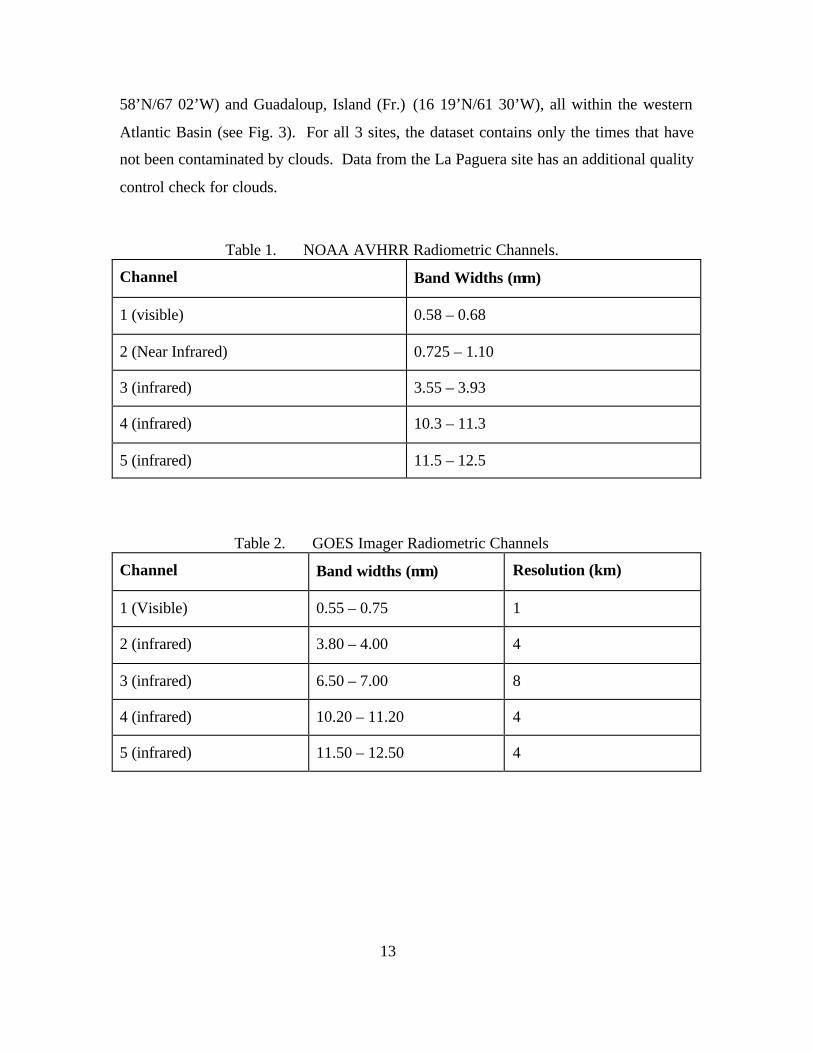
Table 1. NOAA AVHRR Radiometric Channels.
Channel Band Widths (µm)
1 (visible) 0.58 – 0.68
2 (Near Infrared) 0.725 – 1.10
3 (infrared) 3.55 – 3.93
4 (infrared) 10.3 – 11.3
5 (infrared) 11.5 – 12.5
Table 2. GOES Imager Radiometric Channels
Channel Band widths (µm) Resolution (km)
1 (Visible) 0.55 – 0.75 1
2 (infrared) 3.80 – 4.00 4
3 (infrared) 6.50 – 7.00 8
4 (infrared) 10.20 – 11.20 4
5 (infrared) 11.50 – 12.50 4

14
Figure 3. Map of the experimental region with locations of the AERONET stations.

15
IV. METHODOLOGY
A. SELECTION OF CASES
Datasets were collected on a daily basis from the GOES-8, NOAA, and
AERONET instruments. The process started in the middle of July 2001 and lasted until
the end of September 2001. GOES-8 data was collected from a Terascan receiving
platform located at the Naval Research Laboratory, in Monterey, CA. The data was
downloaded in a short (10 bit) format to a UNIX workstation every half-hour. GOES-8
data in August was downloaded into 8 bit instead of the 10 bit format, and was not
suitable for processing. As a result, all data in August was rejected.
NOAA data was readily available through a NOAA NESDIS archives. Of the
two satellite sensors, data from NOAA-16 AVHRR was more suitable than the NOAA-
14 because NOAA-16 orbital passes occurred over the study region (eastern Atlantic and
Caribbean Sea) during the times of interest - late morning through early afternoon.
NOAA-14 orbital passes occurred during the late afternoon and its data was often
rejected because of low sun angles. For both NOAA sensors, datasets were also rejected
when the sun glint pattern (specular solar reflection) covered the study area. The NPS
algorithm identifies and rejects the contaminated region during data processing.
AERONET data was also readily available via NASA’s AERONET archive for
all 3 locations. Cases were rejected if there was insufficient data covering the particular
site during the local afternoon hours. These conditions usually occurred because of the
presence of clouds over the AERONET radiometer’s field of view, which unfortunately,
is a common diurnal occurrence over all 3 islands, especially during the afternoon hours.
Data was manually rejected during times that the observed AOD values showed
tendencies of significant increase before a cloudy episode.
B. GOES-8 CALIBRATION AND CORRECTION PROCESSES
Although extensive studies have shown that the NPS algorithm performed well
with NOAA AVHRR data, the results using GOES-8 data were very limited. For GOES-
8, there is no on-board calibration for the channel 1 radiances. In addition, there was a
problem of non- linear signal degradation immediately after the launch in 1994. There

16
have been several attempts to perform vicarious calibration techniques to adjust for the
weakening signal strength and to take into account the post- launch degradation. There is
an additional problem with noise and signal radiometric resolution generated from GOES
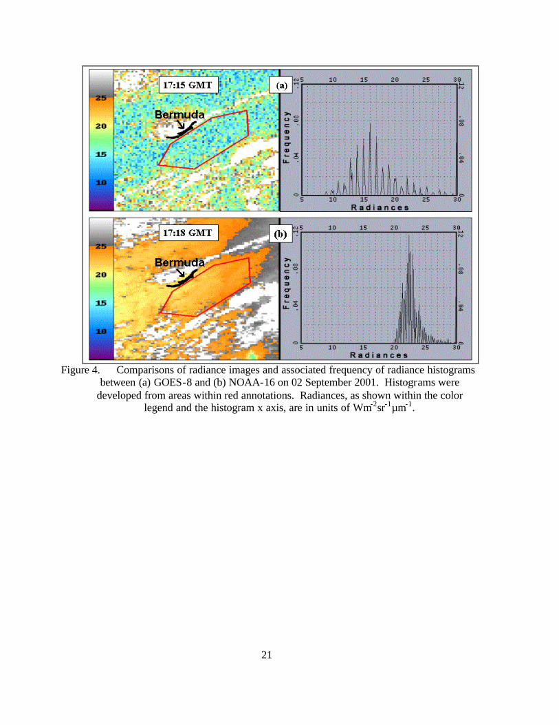
sensors. Figure 4 displays an example of radiance comparisons between the calibrated
GOES and AVHRR datasets. The image passes occurred at a similar time and were
registered over the same 100 km by 100 km domain surrounding Bermuda. In addition,
both satellites had similar viewing geometries (scatter angles were ± 0.1o of each other).
The atmospheric conditions immediately south of Bermuda (outlined in red) were clear
and homogeneous at this time. The panel to the right of Figure 4 are plots of the
histogram frequency distribution of radiances that were extracted within the outlined
region. As expected, the NOAA-16 image in (b) displays a relatively homogeneous field
of radiances; its corresponding frequency histogram displays shows a pronounced signal
peak with a narrow radiometric width, indicative of the pristine atmospheric conditions.
In contrast, the GOES-8 sensor, situated in an orbit that is 40 times the distance of the
NOAA sensor, produces an image (shown in (a)) that is significantly noisier; its
corresponding histogram profile displays a weaker signal peak and wider radiometric
range. As atmospheric conditions become hazier, the GOES-8 peak signal and
radiometric resolutions become even less discernable, thus complicating the processed
AOD calculations. In addition, the GOES-8 signal peak at ~ 16 Wm-2sr-1µm-1 is
significantly weaker than the NOAA-16 signal peak at ~22.5 Wm-2sr-1µm-1, thus
necessitating a further correction factor to GOES-8 for further processing.
For this study, in order to match GOES with NOAA data during AOD processing,
two correction techniques were applied to the GOES channel 1 radiance data. Dr. C. R.
N. Rao (personal communication in July, 2000) developed a calibration methodology of
GOES-8 channel radiance by a vicarious technique, selecting a radiometrically stable
calibration site located in the Sonoran desert (34.0oN/114.1oW). Radiometrically stable
calibration is defined as the long term mean value at the top of the atmosphere albedo that
remains uniform in time. Details of this method can be found in Rao and Zhang (1999)
and Rao et al. (1999).

17
Dr. Rao developed a simplified version of the correction factor (gain factor) that
can be expressed in the following equation:
( )( ) ( )
A d;post_ = = 1.192* 1+1.688E-04*d
A preGAIN FACTOR (8)
where:
d = number of days since the launch date of the GOES-8 satellite
A(pre) = albedo (%) calculated using the pre- launch calibration coefficients
A(d;post) = albedo (%) calculated on day ‘d’ after the launch of GOES-8, that accounts for degradation in orbit)
Table 1 in Appendix A lists the calibration factor applied to GOES-8 for each
case study day in this report. However, a preliminary assessment of the calibrated GOES
data indicated that its resulting AOD values were significantly higher than the NOAA-
generated AOD as well as the AERONET observations of AOD. Therefore, a further
correction method was applied, as discussed below.
The correction technique involved comparisons between GOES-8 and NOAA-16
channel 1 radiances, whose wavelengths, centered on 0.65 and 0.63 µm, respectively,
were similar. The assumption is that the calibrated AVHRR channel 1 radiances are
accurate. The process involved the collection of a sample of cases when the GOES and
NOAA viewing geometries over a selected location were similar. GOES and NOAA
viewing geometries were defined as ‘similar’ when the scatter and azimuth angles were
within ± 0.1o of each other. Figure 5 presents the comparisons over 296 pairs of GOES
and NOAA channel 1 radiances. As shown, the radiance ranged along the low end of the
radiance spectrum (0 to 40 Wm-2sr-1µm-1) which is where the detection of aerosols would
occur. As shown, there was very poor correlation between the NOAA and GOES data,
due to the large noise problem in GOES. As a plausible correction, it was decided to
perform a manually-determined selection of the “center of mass” within the domain
shown in Figure 5. Using the Cartesian coordinates, the selected center of mass of the
distribution was positioned at point Y (NOAA axis) = 24.0 Wm-2sr-1 µm-1 and point X
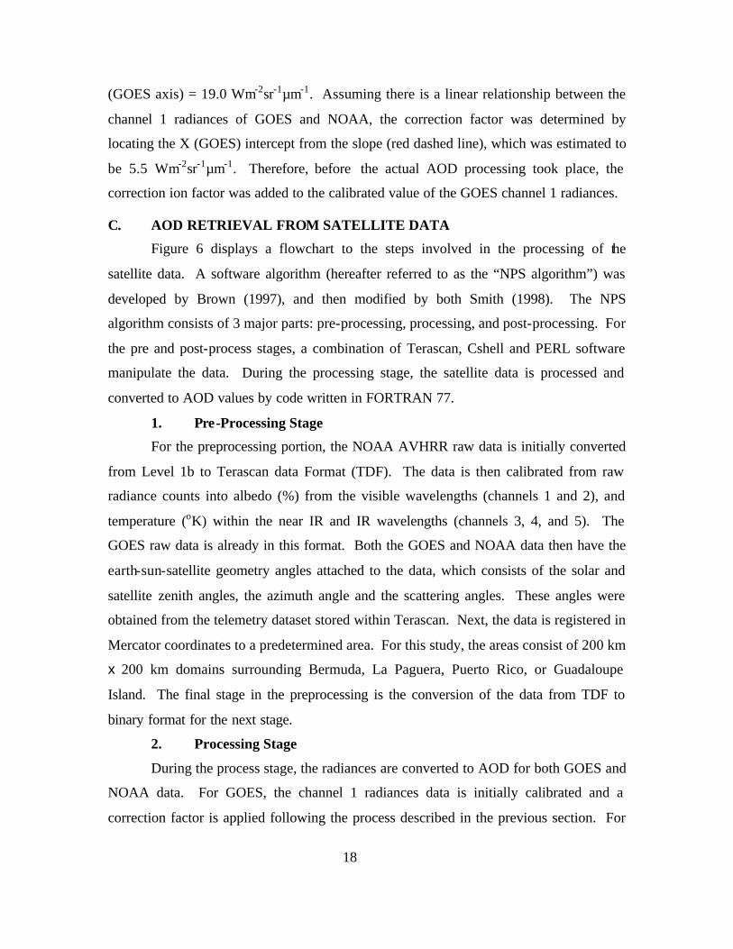
18
(GOES axis) = 19.0 Wm-2sr-1µm-1. Assuming there is a linear relationship between the
channel 1 radiances of GOES and NOAA, the correction factor was determined by
locating the X (GOES) intercept from the slope (red dashed line), which was estimated to
be 5.5 Wm-2sr-1µm-1. Therefore, before the actual AOD processing took place, the
correction ion factor was added to the calibrated value of the GOES channel 1 radiances.
C. AOD RETRIEVAL FROM SATELLITE DATA
Figure 6 displays a flowchart to the steps involved in the processing of the
satellite data. A software algorithm (hereafter referred to as the “NPS algorithm”) was
developed by Brown (1997), and then modified by both Smith (1998). The NPS
algorithm consists of 3 major parts: pre-processing, processing, and post-processing. For
the pre and post-process stages, a combination of Terascan, Cshell and PERL software
manipulate the data. During the processing stage, the satellite data is processed and
converted to AOD values by code written in FORTRAN 77.
1. Pre-Processing Stage
For the preprocessing portion, the NOAA AVHRR raw data is initially converted
from Level 1b to Terascan data Format (TDF). The data is then calibrated from raw
radiance counts into albedo (%) from the visible wavelengths (channels 1 and 2), and
temperature (oK) within the near IR and IR wavelengths (channels 3, 4, and 5). The
GOES raw data is already in this format. Both the GOES and NOAA data then have the
earth-sun-satellite geometry angles attached to the data, which consists of the solar and
satellite zenith angles, the azimuth angle and the scattering angles. These angles were
obtained from the telemetry dataset stored within Terascan. Next, the data is registered in
Mercator coordinates to a predetermined area. For this study, the areas consist of 200 km
x 200 km domains surrounding Bermuda, La Paguera, Puerto Rico, or Guadaloupe
Island. The final stage in the preprocessing is the conversion of the data from TDF to
binary format for the next stage.
2. Processing Stage
During the process stage, the radiances are converted to AOD for both GOES and
NOAA data. For GOES, the channel 1 radiances data is initially calibrated and a
correction factor is applied following the process described in the previous section. For

19
both datasets, sun glint contamination is removed by applying a method used by Cox and
Munk (1954).
AOD is calculated following Eq. (2),
( )( )( )
4µLad = a ? F p ?o o s.
The cosine of the satellite zenith angle (µ), the single-scatter albedo (? o), and the solar
radiance (Fo) are all constants. Radiance due to aerosol scatter (La), is mathematically
straightforward and is described in detail by Brown (1997). The scattering phase
function, p(? s), is obtained from a process described below.
a. Scattering Phase Function Processing
Obtaining the scattering phase function values requires knowledge of the
aerosol characteristics and size distribution, which is not routinely available. Therefore,
the scattering phase function must be parameterized. Durkee et al. (1991) developed the
parameterization technique used within the NPS algorithm. The technique consists of
calculating the ratio of the NOAA channel 1 and 2 radiances, ‘S12’. The scattering
efficiency (Qscat) of an aerosol distribution is wavelength dependent and peaks when the
radius of the aerosol particle is nearly equal to that of the radiation wavelength. As a
result, S12 will be larger for smaller size particle distributions and smaller for larger size
aerosol particle distributions. S12 varies from pixel to pixel. Therefore, variations in the
aerosol size distribution can be detected within the pixel resolutions of the satellite image
data.
Brown (1997) generated seven models of aerosol size distributions. These
models typify general conditions within the maritime environment. The scattering phase
function and extinctions for these models were calculated using Mie theory. Table 3
describes the attributes for each of the 7 models. These distributions consist of one
single-mode and 6 two-mode log normal distributions with varying radii and standard
deviations used to describe variations of aerosol distribution widths in the maritime
atmosphere. Figures 7, 8, and 9 illustrate the effect of the aerosol size distribution
models on S12 and the scattering phase function (developed by Brown, 1997). Figure 10

20
is a composite chart that illustrates the actual phase function extraction process. This
process only applies to NOAA processing. For each pixel, the combination of the scatter
angle and the computed S12 value is entered into a lookup table (LUT) represented in the
upper left portion of Figure 10 to determine the model aerosol distribution that is
consistent with the measured S12. An aerosol model index (AMI) is interpolated between
models M0 and M6. In the example shown, the interpola ted value is situated between
Models M2 and M3 (i.e., AMI is approximately 2.5). The AMI values are collected for
each pixel and stored in a file. During the GOES processing, this data from the AMI file
is accessed. For both GOES and NOAA processes, the next and final step to the NOAA
phase function processing is entering the AMI value with the scatter angle to the
scattering phase function LUT, as graphically represented in Figure 4.4 and in the lower
left portion of Figure 10. For GOES processing, the AMI values are assumed to be
constant during the entire time period. At this stage, all of the input parameters have
been determined and the AOD is calculated using Eq. (2).
3. Post-Processing Stage
During the post-processing stage, all of the original channel data, calculated data,
and extracted scattering phase function values are reformatted back to TDF; this data is in
image form and can then be viewed and analyzed via the Terascan visualization software.
Table 4 lists the output products generated by the NPS algorithm. For this study, only the
channel 1 AOD is calculated for the case study analysis.
21
Figure 4. Comparisons of radiance images and associated frequency of radiance histograms
between (a) GOES-8 and (b) NOAA-16 on 02 September 2001. Histograms were developed from areas within red annotations. Radiances, as shown within the color
legend and the histogram x axis, are in units of Wm-2sr-1µm-1.
22
Figure 5. Comparisons of Channel 1 radiances between GOES-8 and NOAA-16.
Radiances are in units of Wm-2sr-1µm-1.

23
Figure 6. Satellite AOD retrieval process (portions obtained from Brown, 1997).

24
Figure 7. Model aerosol size distributions (from Brown, 1997).
25
Figure 8. Model phase functions for NOAA’s channel 1 (visible wavelength) (from Brown,
1997).
Figure 9. Model S12 values (from Brown, 1997).
26
Figure 10. Parameterization of the scattering phase function, p(? s), is described. (a) Aerosol
model size distributions. (b) size index, S12, (c) scattering phase function calculated from the model size distributions as a function of scattering angle. (portions of figure obtained
from Durkee et al., 1999.)
27
Table 3. Characteristics for each of the 7 models of the aerosol size distribution. Mode 1 models the background aerosols while Mode 2 models the ocean-produced aerosols.
Model Mode Radii (µm)
Mode 1 Mode 2
Number density (N)
Mode 1 Mode 2
Std dev (s)
Mode 1 Mode 2
M0 0.1 0.0 1000 0 1.7 0.00
M1 0.1 0.3 1000 3 1.7 2.10
M2 0.1 0.3 1000 5 1.7 2.20
M3 0.1 0.3 1000 8 1.7 2.35
M4 0.1 0.3 1000 10 1.7 2.51
M5 0.1 0.3 1000 13 1.7 2.60
M6 0.1 0.3 1000 15 1.7 2.70
Table 4. List of the output products for each pixel within the image file as generated by the
NPS algorithm for both GOES and NOAA data processes.
GOES-8 products NOAA-14 and 16 products Channel 1 total radiance Channel 1 total radiance Channel 2 total radiances
Channel 1 Rayleigh radiance Channel 1 Rayleigh radiance
Channel 2 Rayleigh radiance
Channel 1 aerosol radiance Channel 1 aerosol radiance Channel 2 aerosol radiance
Satellite zenith angles Satellite zenith angles
Solar zenith angles Solar zenith angles
Relative azimuth angles Relative azimuth angles
Scatter angles Scatter angles
Channel 1 phase functions Channel 1 phase functions Channel 2 phase functions
Channel 1 AOD Channel 1 AOD Channel 2 AOD
Ratio of channel1 and channel2 (S12)
Aerosol Model Index (AMI)

28
THIS PAGE INTENTIONALLY LEFT BLANK
29
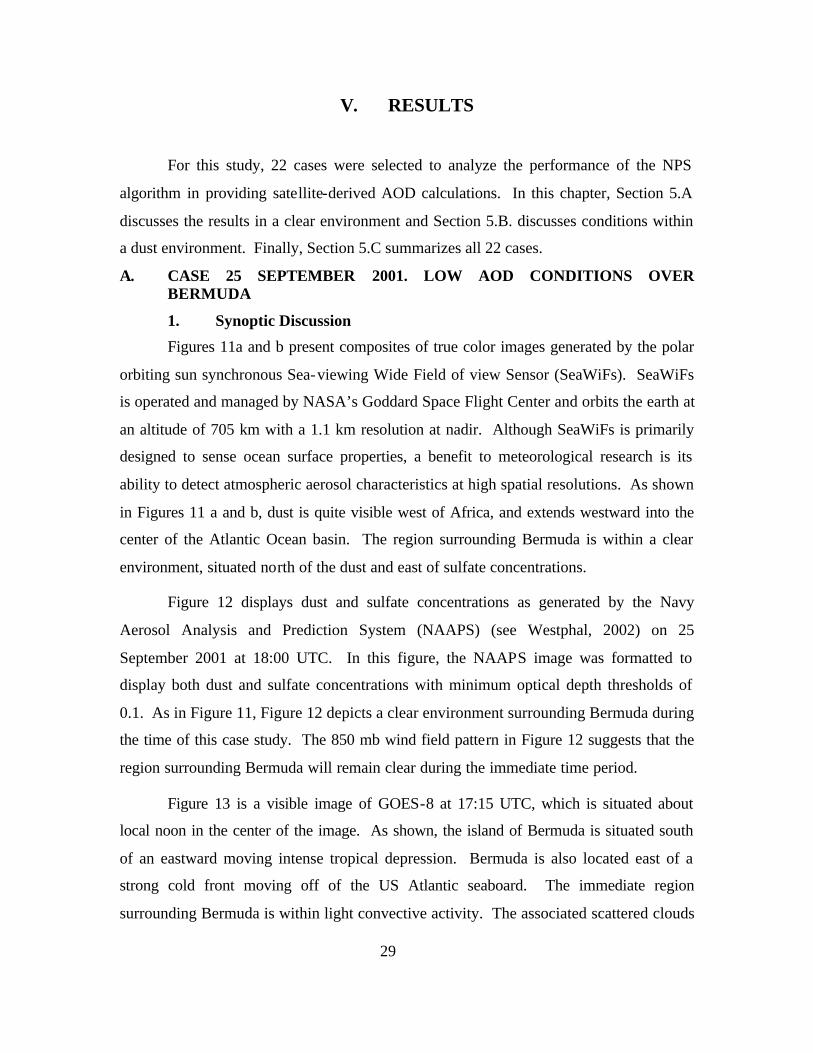
V. RESULTS
For this study, 22 cases were selected to analyze the performance of the NPS
algorithm in providing satellite-derived AOD calculations. In this chapter, Section 5.A
discusses the results in a clear environment and Section 5.B. discusses conditions within
a dust environment. Finally, Section 5.C summarizes all 22 cases.
A. CASE 25 SEPTEMBER 2001. LOW AOD CONDITIONS OVER BERMUDA
1. Synoptic Discussion
Figures 11a and b present composites of true color images generated by the polar
orbiting sun synchronous Sea-viewing Wide Field of view Sensor (SeaWiFs). SeaWiFs
is operated and managed by NASA’s Goddard Space Flight Center and orbits the earth at
an altitude of 705 km with a 1.1 km resolution at nadir. Although SeaWiFs is primarily
designed to sense ocean surface properties, a benefit to meteorological research is its
ability to detect atmospheric aerosol characteristics at high spatial resolutions. As shown
in Figures 11 a and b, dust is quite visible west of Africa, and extends westward into the
center of the Atlantic Ocean basin. The region surrounding Bermuda is within a clear
environment, situated north of the dust and east of sulfate concentrations.
Figure 12 displays dust and sulfate concentrations as generated by the Navy
Aerosol Analysis and Prediction System (NAAPS) (see Westphal, 2002) on 25
September 2001 at 18:00 UTC. In this figure, the NAAPS image was formatted to
display both dust and sulfate concentrations with minimum optical depth thresholds of
0.1. As in Figure 11, Figure 12 depicts a clear environment surrounding Bermuda during
the time of this case study. The 850 mb wind field pattern in Figure 12 suggests that the
region surrounding Bermuda will remain clear during the immediate time period.
Figure 13 is a visible image of GOES-8 at 17:15 UTC, which is situated about
local noon in the center of the image. As shown, the island of Bermuda is situated south
of an eastward moving intense tropical depression. Bermuda is also located east of a
strong cold front moving off of the US Atlantic seaboard. The immediate region
surrounding Bermuda is within light convective activity. The associated scattered clouds
30
remain around the island throughout the day, but did not impact the AOD calculations
conducted over water just east of the island.
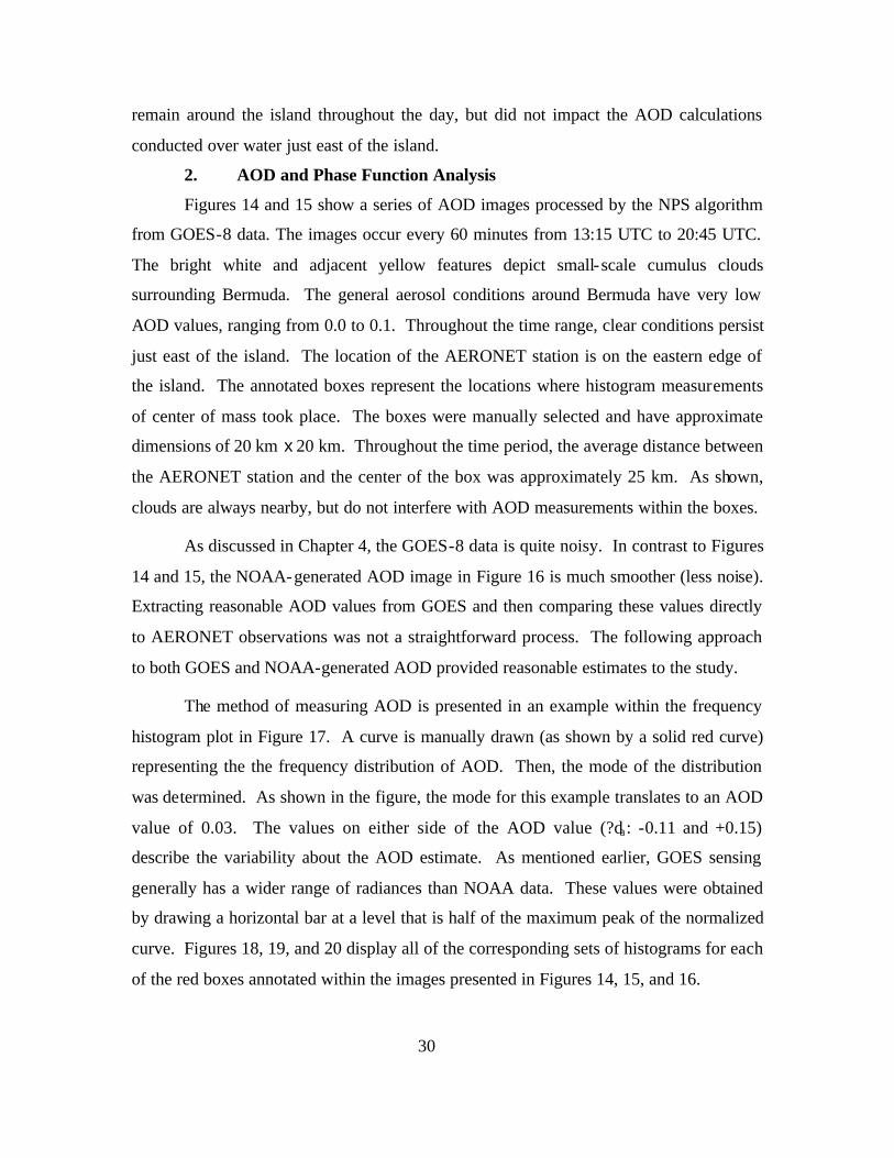
2. AOD and Phase Function Analysis
Figures 14 and 15 show a series of AOD images processed by the NPS algorithm
from GOES-8 data. The images occur every 60 minutes from 13:15 UTC to 20:45 UTC.
The bright white and adjacent yellow features depict small-scale cumulus clouds
surrounding Bermuda. The general aerosol conditions around Bermuda have very low
AOD values, ranging from 0.0 to 0.1. Throughout the time range, clear conditions persist
just east of the island. The location of the AERONET station is on the eastern edge of
the island. The annotated boxes represent the locations where histogram measurements
of center of mass took place. The boxes were manually selected and have approximate
dimensions of 20 km x 20 km. Throughout the time period, the average distance between
the AERONET station and the center of the box was approximately 25 km. As shown,
clouds are always nearby, but do not interfere with AOD measurements within the boxes.
As discussed in Chapter 4, the GOES-8 data is quite noisy. In contrast to Figures
14 and 15, the NOAA-generated AOD image in Figure 16 is much smoother (less noise).
Extracting reasonable AOD values from GOES and then comparing these values directly
to AERONET observations was not a straightforward process. The following approach
to both GOES and NOAA-generated AOD provided reasonable estimates to the study.
The method of measuring AOD is presented in an example within the frequency
histogram plot in Figure 17. A curve is manually drawn (as shown by a solid red curve)
representing the the frequency distribution of AOD. Then, the mode of the distribution
was determined. As shown in the figure, the mode for this example translates to an AOD
value of 0.03. The values on either side of the AOD value (?da: -0.11 and +0.15)
describe the variability about the AOD estimate. As mentioned earlier, GOES sensing
generally has a wider range of radiances than NOAA data. These values were obtained
by drawing a horizontal bar at a level that is half of the maximum peak of the normalized
curve. Figures 18, 19, and 20 display all of the corresponding sets of histograms for each
of the red boxes annotated within the images presented in Figures 14, 15, and 16.

31
Figure 21 presents the time series plot of AOD obtained from Figures 18, 19, and
20. There is one NOAA measurement obtained at 18:16 UTC. “Variability” bars are
plotted for each measurement. Because of the inherent noise within the GOES-8
radiances, the variability of AOD is significantly higher for GOES-8 (?d: +/- 0.10 to
0.15) than NOAA data (?d: +/- 0.02). Although AOD values can never fall below zero,
the first two GOES points (Time = 13:15 UTC and 13:45 UTC) produce slightly negative
AOD values, due again to the noise associated with GOES data. As shown, there is good
agreement between the AERONET and GOES-derived AOD after about 17:00 UTC.
The AVHRR-derived AOD value of 0.12 is significantly greater than the corresponding
AERONET observed value of ~0.05 at 18:16 UTC. Included within Figure 21 is the
scatter angle pattern shown in a dashed line. Because of the geometric configuration
between the sun and GOES-8 satellite, local noon occurs approximately where the scatter
angle position is at its peak, which is also the closest to a direct backscatter configuration
between the sun and satellite sensor. As time increases, the GOES-8 – sun geometry
results in more of a side scatter. This geometry affects the phase function determination,
which is discussed below.
Figure 22 displays the phase function values generated from both the NPS
algorithm and AERONET observations. The satellite-derived phase function values
(blue diamonds) are obtained from the algorithm’s lookup table, as described in
Chapter 4. The corresponding red square at each scatter angle represents the phase
function value required for the satellite-derived AOD to match AERONET AOD. As
shown, all values are within the backscatter portion (90o – 180o). This figure provides an
evaluation tool to determine the proper phase function pattern, given the aerosol
conditions for a particular case. In this case, the AERONET phase function values are
consistently lower than the satellite-derived phase functions.
B. CASE 18 SEPTEMBER 2001. HIGH AOD CONDITIONS OVER GUADALOUPE ISLAND
1. Synoptic Discussion
During the summer months, dust generated from the African deserts are often
propagated across the southern latitudes of the Atlantic Ocean basin by the easterly trade
winds, oftentimes impacting the visibility and aerosol characteristics over regions of the
32
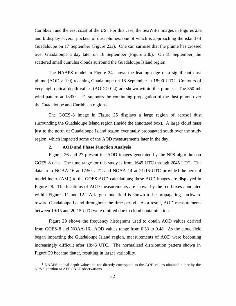
Caribbean and the east coast of the US. For this case, the SeaWiFs images in Figures 23a
and b display several pockets of dust plumes, one of which is approaching the island of
Guadaloupe on 17 September (Figure 23a). One can surmise that the plume has crossed
over Guadaloupe a day later on 18 September (Figure 23b). On 18 September, the
scattered small cumulus clouds surround the Guadaloupe Island region.
The NAAPS model in Figure 24 shows the leading edge of a significant dust
plume (AOD > 1.0) reaching Guadaloupe on 18 September at 18:00 UTC. Contours of
very high optical depth values (AOD > 0.4) are shown within this plume.1 The 850 mb
wind pattern at 18:00 UTC supports the continuing propagation of the dust plume over
the Guadaloupe and Caribbean regions.
The GOES-8 image in Figure 25 displays a large region of aerosol dust
surrounding the Guadaloupe Island region (inside the annotated box). A large cloud mass
just to the north of Guadaloupe Island region eventually propagated south over the study
region, which impacted some of the AOD measurements later in the day.
2. AOD and Phase Function Analysis
Figures 26 and 27 present the AOD images generated by the NPS algorithm on
GOES-8 data. The time range for this study is from 1645 UTC through 2045 UTC. The
data from NOAA-16 at 17:50 UTC and NOAA-14 at 21:16 UTC provided the aerosol
model index (AMI) to the GOES AOD calculations; these AOD images are displayed in
Figure 28. The locations of AOD measurements are shown by the red boxes annotated
within Figures 11 and 12. A large cloud field is shown to be propagating southward
toward Guadaloupe Island throughout the time period. As a result, AOD measurements
between 19:15 and 20:15 UTC were omitted due to cloud contamination.
Figure 29 shows the frequency histograms used to obtain AOD values derived
from GOES-8 and NOAA-16. AOD values range from 0.33 to 0.48. As the cloud field
began impacting the Guadaloupe Island region, measurements of AOD were becoming
increasingly difficult after 18:45 UTC. The normalized distribution pattern shown in
Figure 29 became flatter, resulting in larger variability.
1 NAAPS optical depth values do not directly correspond to the AOD values obtained either by the
NPS algorithm or AERONET observations.

33
Figure 30 presents the time series of AOD for this case. Both the GOES-
generated AOD and the AERONET observations of AOD are in good agreement, with
high AOD values throughout the time period. As mentioned earlier, cloud contamination
resulted in limited AOD measurements after 19:15 UTC. The lengths of the variability
bars associated with GOES-8 data increased with time. As a result, the proper selection
of AOD measurements became increasingly more difficult. The AOD generated from the
NOAA-16 data at 17:50 UTC (AOD ~ 0.45) and the NOAA-14 data at 21:17 UTC (AOD
~ 0.48) are also in agreement with AERONET observations. Based on the scatter angle
profile, local noon occurred toward the beginning of the time period (~16:45 UTC). The
AOD from AERONET observations tend toward higher values than the satellite-derived
AOD during the early afternoon hours. The reverse occurs later in the day.
Figure 31 displays the phase function value profiles from satellite and AERONET
data. As in the previous case (Figure 22), the AERONET phase function values are
consistently lower than the satellite-derived phase functions. Due to the limited dataset,
there was not a distinct phase function pattern to describe this dust environment. The
next chapter will address this issue more clearly.
C. RESULTS FROM 22 CASES
Table 1 in Appendix A lists the dates, times and locations of all of the cases in
this study. The data was selected based on the availability of both satellite and
AERONET data. Also, entire case study days were rejected when the NOAA data was
contaminated by sun glint within the region of study.
Appendix B presents the AOD charts for all 22 cases. Most of the cases have
AOD profiles that are fairly dust- free (da < 2.5). The exceptions are cases 2, 7, 8, 12, 14,
16, and 20. Unfortunately, for the high dust cases, data for the analysis is usually limited
because there tends to be more cloud contamination surrounding all 3 islands within the
study. As a result the contaminated data are filtered out of the case studies. Within the
GOES-8 data, local noon occurs during the peak of the scatter angle, between 16:45 and
17:15 UTC in September. During the late afternoon hours, the AOD profile becomes
more questionable, as shadows from nearby clouds might affect the clear regions.
Special care was taken to avoid these problem areas.
34
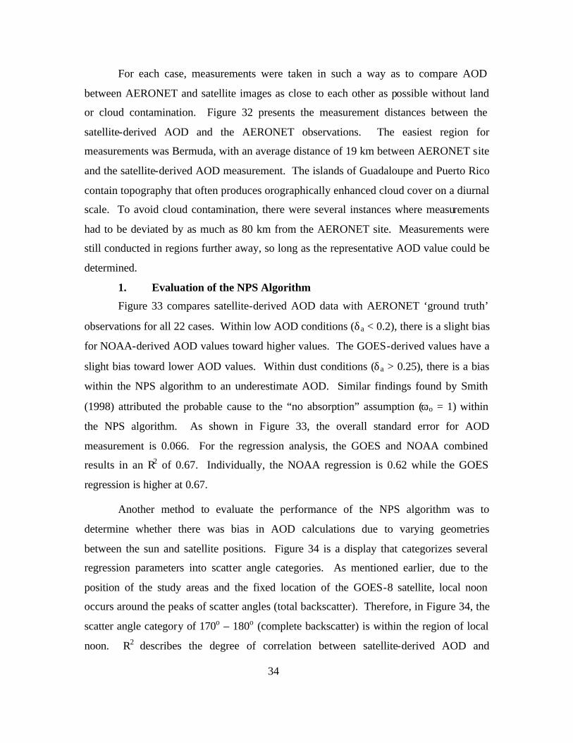
For each case, measurements were taken in such a way as to compare AOD
between AERONET and satellite images as close to each other as possible without land
or cloud contamination. Figure 32 presents the measurement distances between the
satellite-derived AOD and the AERONET observations. The easiest region for
measurements was Bermuda, with an average distance of 19 km between AERONET site
and the satellite-derived AOD measurement. The islands of Guadaloupe and Puerto Rico
contain topography that often produces orographically enhanced cloud cover on a diurnal
scale. To avoid cloud contamination, there were several instances where measurements
had to be deviated by as much as 80 km from the AERONET site. Measurements were
still conducted in regions further away, so long as the representative AOD value could be
determined.
1. Evaluation of the NPS Algorithm
Figure 33 compares satellite-derived AOD data with AERONET ‘ground truth’
observations for all 22 cases. Within low AOD conditions (δa < 0.2), there is a slight bias
for NOAA-derived AOD values toward higher values. The GOES-derived values have a
slight bias toward lower AOD values. Within dust conditions (δa > 0.25), there is a bias
within the NPS algorithm to an underestimate AOD. Similar findings found by Smith
(1998) attributed the probable cause to the “no absorption” assumption (ωo = 1) within
the NPS algorithm. As shown in Figure 33, the overall standard error for AOD
measurement is 0.066. For the regression analysis, the GOES and NOAA combined
results in an R2 of 0.67. Individually, the NOAA regression is 0.62 while the GOES
regression is higher at 0.67.
Another method to evaluate the performance of the NPS algorithm was to
determine whether there was bias in AOD calculations due to varying geometries
between the sun and satellite positions. Figure 34 is a display that categorizes several
regression parameters into scatter angle categories. As mentioned earlier, due to the
position of the study areas and the fixed location of the GOES-8 satellite, local noon
occurs around the peaks of scatter angles (total backscatter). Therefore, in Figure 34, the
scatter angle category of 170o – 180o (complete backscatter) is within the region of local
noon. R2 describes the degree of correlation between satellite-derived AOD and
35
AERONET data. For example, R2 = 0.40, indicates that 40% of the original variability of
the satellite-derived AOD can be explained, with a remaining 60% of residual variability.
As shown within the bar patterns of Figure 34, R2 values are highest about 140o – 150o
(R2 ~ 0.72) and at 170o - 180o (R2 ~ 0.76). Corresponding standard error (S.E.) values are
at their lowest within the scatter angle categories of 130o - 140o and 170o - 180o,
respectively. A possible explanation for the higher accuracy about 140 degrees could be
that the model phase function table of values used within the NPS algorithm converge
toward one value at ~140 degrees. Therefore, there are no aerosol size distribution
selection errors at this scatter angle.
Figure 35 displays the phase function analysis for the 22 cases within dust
conditions (δa = 0.25). Satellite-derived phase functions (blue dots) and the phase
functions required to match the AERONET AOD (red dots) are shown. Between 140o
and 180o, phase function values generated by the NPS algorithm indicate a pattern of
higher curvature than that of AERONET-based phase functions. This result is consistent
with work conducted by Collins et al. (2000) in the ACE-2 experiment off the west
African coast (upstream from the PRIDE region). Figure 36 presents their findings.
Beyond the scatter angle of 140o, non-spherical dust particles were observed to produce a
flatter phase function shape than non-dust conditions. Figure 37 shows the 7 aerosol size
distribution models used in the NPS algorithm with the normalized phase function
patterns supplied by Collins et al. (2000). As shown, within the forward scatter angles
(0o – 90o), both the spherical and non-spherical contours follow the phase function
patterns of the 7 models. However, within the backscatter region (90o – 180o), the non-
spherical phase function curve deviates from all other curves by revealing a flatter
profile. As mentioned earlier, the NPS algorithm applies its theory based on non-dust,
spherical aerosol particles. Based on Figure 37, it would be plausible to apply to the NPS
algorithm a modified phase function that is flatter in the backscatter region during dust
events.
36
(a)
(b)
Figure 11. Composite of SeaWiFs images centered at 12 UTC on (a) 24 September, 2001
and (b) 25 September 2001 covering the Atlantic Basin. The location of interest for this study is the island of Bermuda. Over the ocean, clear (low aerosol content) regions are in
dark blue, cloudy regions are solid white, and gray regions depict higher aerosol (dust) content. A large plume of dust is visible off of the west coast of Africa. (Courtesy of Dr.
Douglas L. Westphal at NRL)

37
Figure 12. Plot of NAAPS display of optical depth for sulfate (red shades), dust and smoke
(green and yellow shades) over the Atlantic Ocean basin for 25 September 2001, 18:00 UTC. The bottom color bar shows the AOD range for dust and smoke. 850 mb model-generated wind barbs are also displayed. (Courtesy of Dr. Douglas L. Westphal at NRL)

38
Figure 13. GOES-8 visible image on 25 September 2001 at 17:15 UTC. The annotated box
surrounds the region of Bermuda.
39
Figure 14. Time series of AOD images generated for 25 September 2001 from GOES-8 data
that surrounds Bermuda. Pixel sizes are 1.1 km by 1.1 km and the domain is approximately 110 km by 110 km. The times range from 13:15 UTC to 16:15 UTC. Red boxes depict locations where the representative AOD for that area was measured. AOD
color contours are defined on the left side of each image.
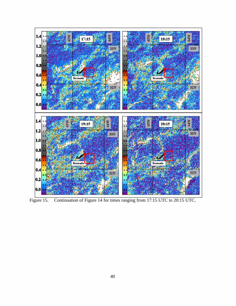
40
Figure 15. Continuation of Figure 14 for times ranging from 17:15 UTC to 20:15 UTC.

41
Figure 16. AOD image generated for 25 September 2001 at 18:17 UTC from NOAA-16 data
that surrounds Bermuda. Pixel sizes are 1.1 km by 1.1 km and the domain is approximately 110 km by 110 km. Red box depicts the location where the representative AOD for that area was measured. AOD color contours are defined on the left side of the
image.
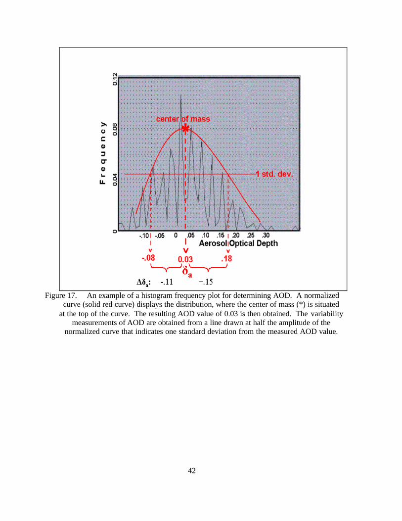
42
Figure 17. An example of a histogram frequency plot for determining AOD. A normalized
curve (solid red curve) displays the distribution, where the center of mass (*) is situated at the top of the curve. The resulting AOD value of 0.03 is then obtained. The variability
measurements of AOD are obtained from a line drawn at half the amplitude of the normalized curve that indicates one standard deviation from the measured AOD value.
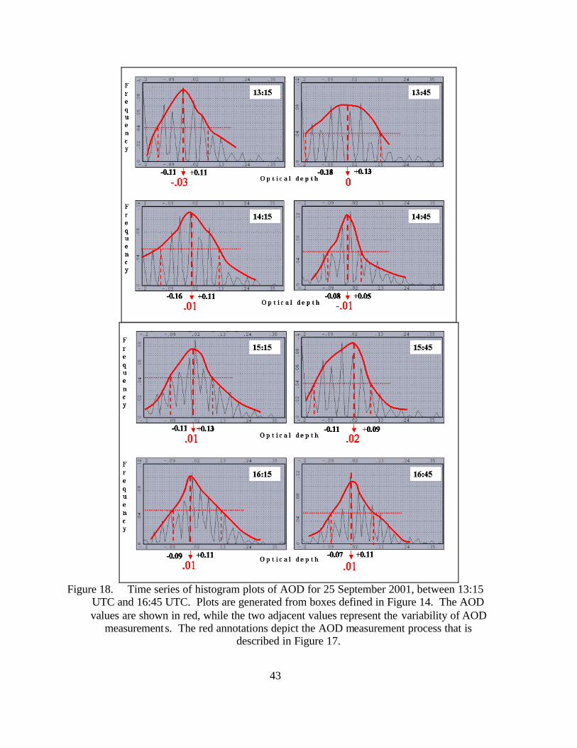
43
Figure 18. Time series of histogram plots of AOD for 25 September 2001, between 13:15
UTC and 16:45 UTC. Plots are generated from boxes defined in Figure 14. The AOD values are shown in red, while the two adjacent values represent the variability of AOD
measurements. The red annotations depict the AOD measurement process that is described in Figure 17.
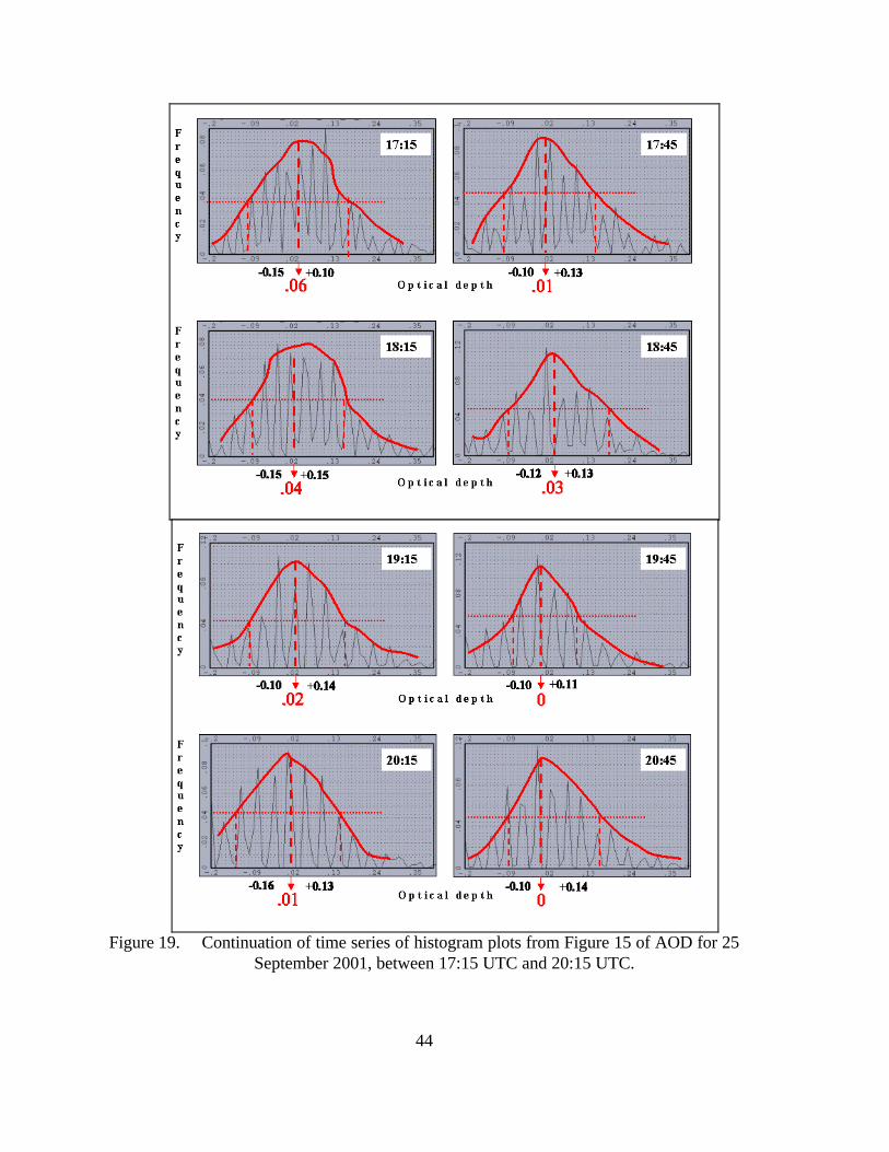
44
Figure 19. Continuation of time series of histogram plots from Figure 15 of AOD for 25
September 2001, between 17:15 UTC and 20:15 UTC.
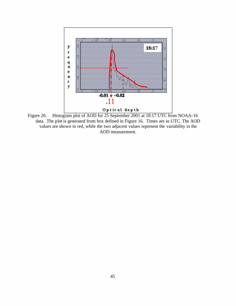
45
Figure 20. Histogram plot of AOD for 25 September 2001 at 18:17 UTC from NOAA-16
data. The plot is generated from box defined in Figure 16. Times are in UTC. The AOD values are shown in red, while the two adjacent values represent the variability in the
AOD measurement.
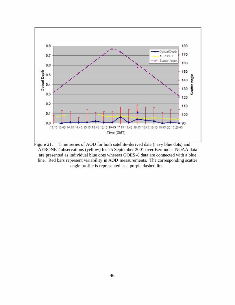
46
Figure 21. Time series of AOD for both satellite-derived data (navy blue dots) and
AERONET observations (yellow) for 25 September 2001 over Bermuda. NOAA data are presented as individual blue dots whereas GOES-8 data are connected with a blue line. Red bars represent variability in AOD measurements. The corresponding scatter
angle profile is represented as a purple dashed line.
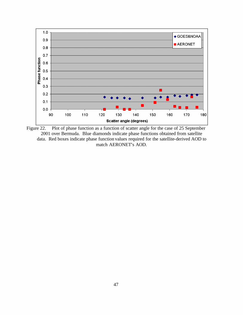
47
Figure 22. Plot of phase function as a function of scatter angle for the case of 25 September
2001 over Bermuda. Blue diamonds indicate phase functions obtained from satellite data. Red boxes indicate phase function values required for the satellite-derived AOD to
match AERONET’s AOD.
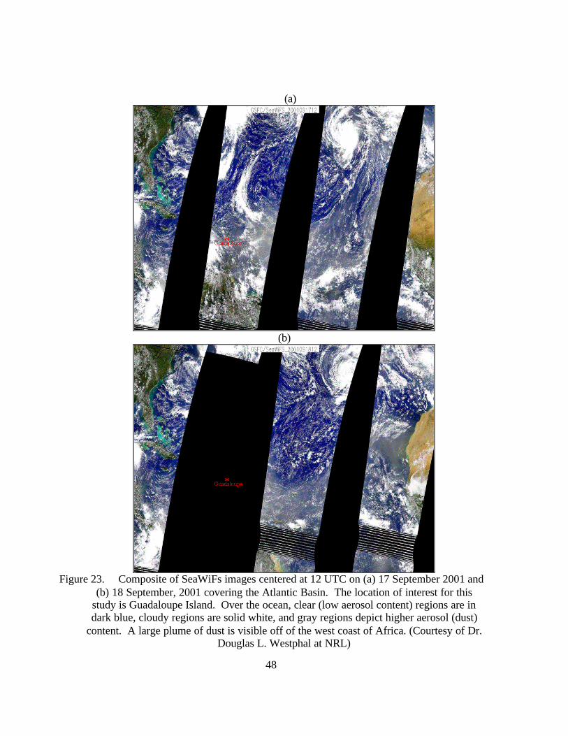
48
(a)
(b)
Figure 23. Composite of SeaWiFs images centered at 12 UTC on (a) 17 September 2001 and
(b) 18 September, 2001 covering the Atlantic Basin. The location of interest for this study is Guadaloupe Island. Over the ocean, clear (low aerosol content) regions are in dark blue, cloudy regions are solid white, and gray regions depict higher aerosol (dust)
content. A large plume of dust is visible off of the west coast of Africa. (Courtesy of Dr. Douglas L. Westphal at NRL)

49
Figure 24. Plot of NAAPS display of optical depth for sulfate (red shades), dust and smoke
(green and yellow shades) over the Atlantic Ocean basin for 18 September 2001, 18:00 UTC. (Courtesy of Dr. Douglas L. Westphal at NRL)

50
Figure 25. GOES-8 visible image on 18 September 2000 at 17:15 UTC. The annotated box
surrounds the region of Guadaloupe Island. The area of aerosol dust is also annotted.

51
Figure 26. Time series of AOD images generated for 18 September 2001 from GOES-8 data
that surrounds Guadaloupe Island. Pixel sizes are 1.1 km by 1.1 km and the domain is approximately 110 km by 110 km. The times range from 16:45 UTC to 18:15 UTC. Red boxes depict locations where the representative AOD for that area was measured. AOD
color contours are defined on the left side of each image.

52
Figure 27. Continuation of Figure 26 for times ranging from 19:15 UTC to 20:45 UTC.
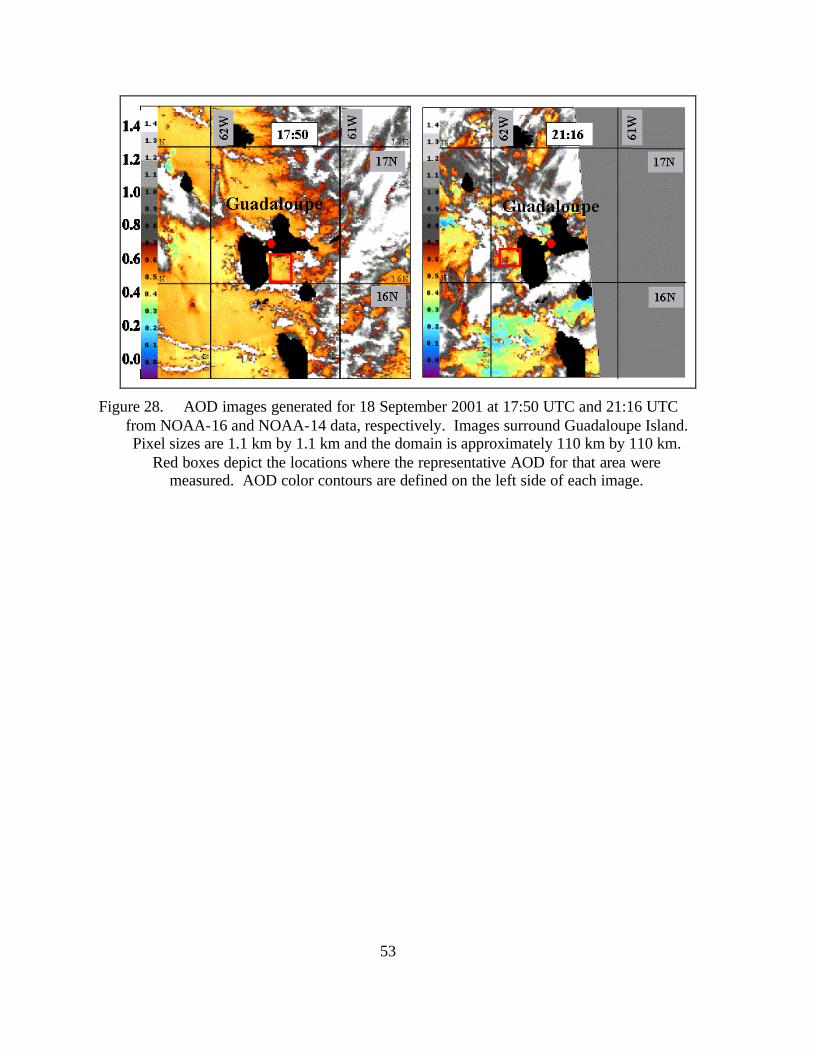
53
Figure 28. AOD images generated for 18 September 2001 at 17:50 UTC and 21:16 UTC
from NOAA-16 and NOAA-14 data, respectively. Images surround Guadaloupe Island. Pixel sizes are 1.1 km by 1.1 km and the domain is approximately 110 km by 110 km.
Red boxes depict the locations where the representative AOD for that area were measured. AOD color contours are defined on the left side of each image.
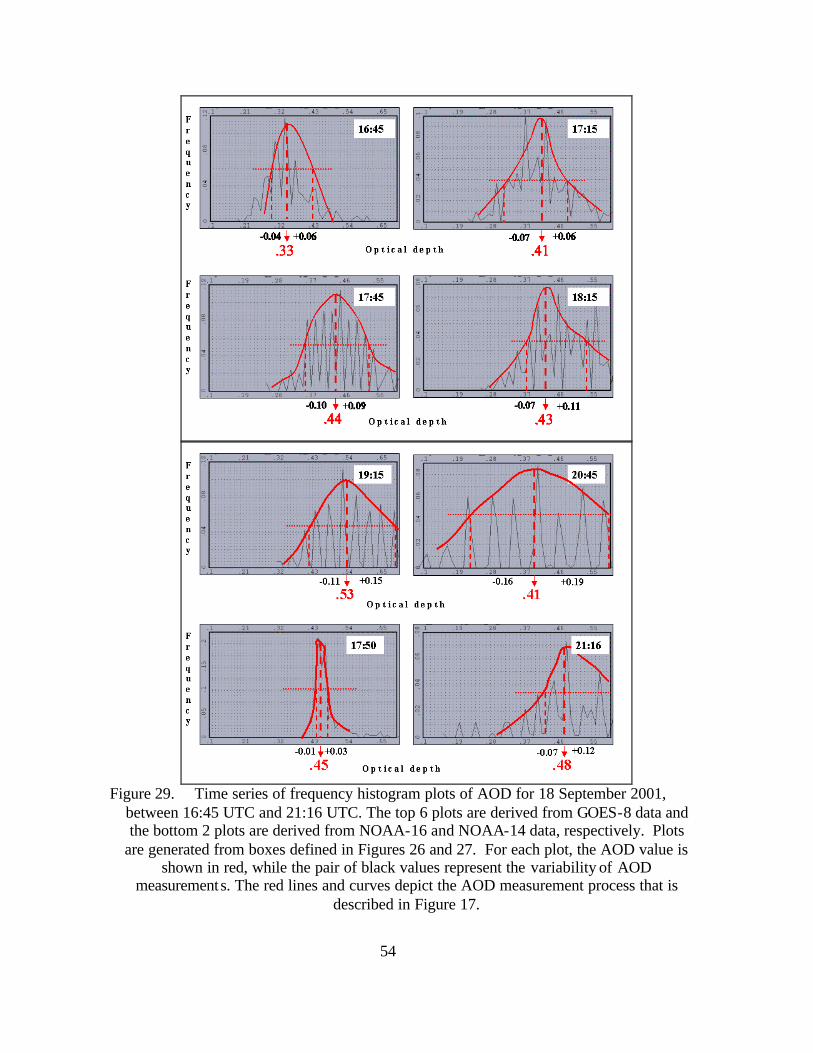
54
Figure 29. Time series of frequency histogram plots of AOD for 18 September 2001,
between 16:45 UTC and 21:16 UTC. The top 6 plots are derived from GOES-8 data and the bottom 2 plots are derived from NOAA-16 and NOAA-14 data, respectively. Plots
are generated from boxes defined in Figures 26 and 27. For each plot, the AOD value is shown in red, while the pair of black values represent the variability of AOD
measurements. The red lines and curves depict the AOD measurement process that is described in Figure 17.

55
Figure 30. Chart of AOD for both satellite-derived data (navy blue dots) and AERONET
observations (yellow) for 18 September 2001 over Guadaloupe Island. NOAA data are presented as individual blue dots whereas GOES-8 data are connected with a blue line. Red bars represent variability in AOD measurements. The corresponding scatter angle
profile is represented as a purple dashed line.
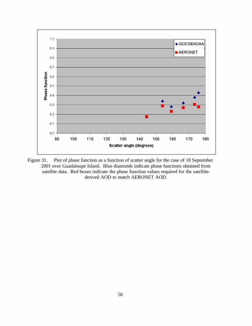
56
Figure 31. Plot of phase function as a function of scatter angle for the case of 18 September
2001 over Guadaloupe Island. Blue diamonds indicate phase functions obtained from satellite data. Red boxes indicate the phase function values required for the satellite-
derived AOD to match AERONET AOD.

57
Figure 32. Distribution of distance measurements between each of the 3 AERONET sites
and the location of the satellite-derived AOD for all 22 cases. For each AERONET region, the average distance from the AERONET station to the center of the satellite-
derived measurement box is annotated in red.
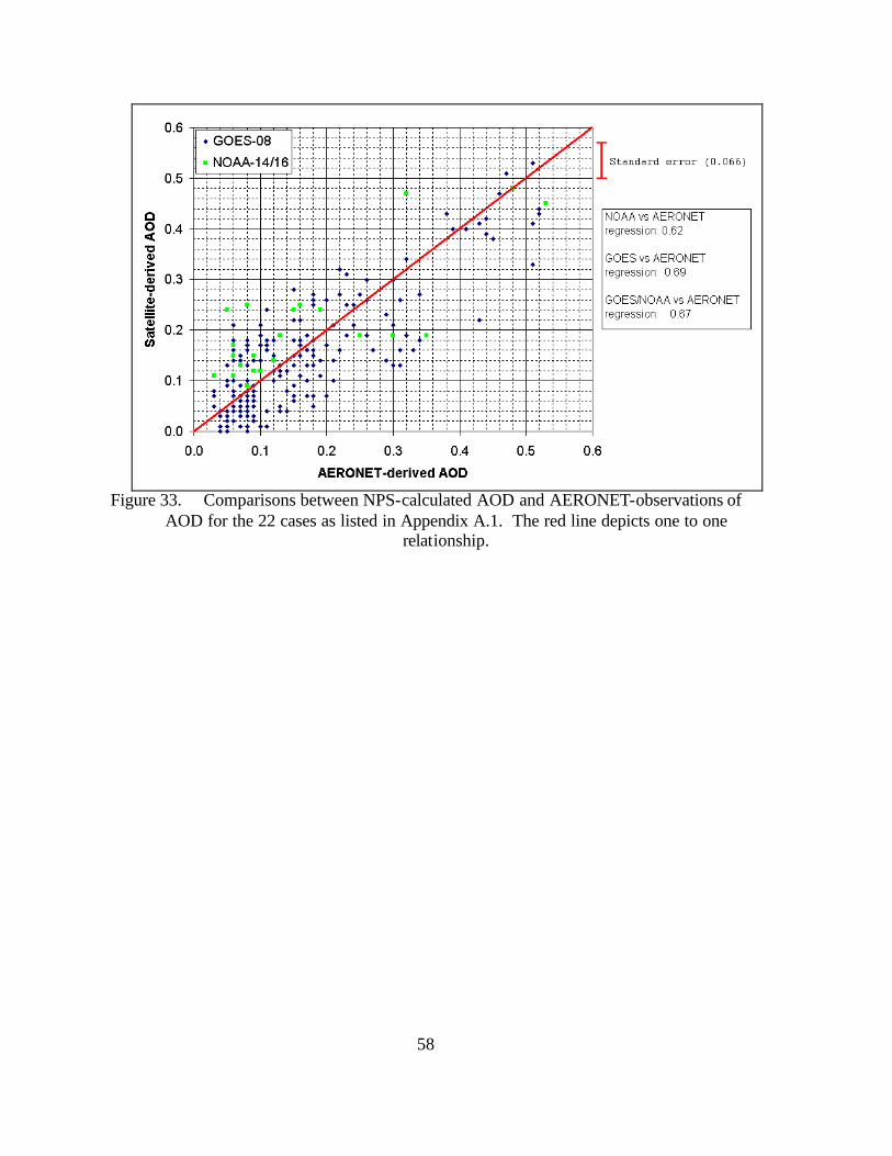
58
Figure 33. Comparisons between NPS-calculated AOD and AERONET-observations of
AOD for the 22 cases as listed in Appendix A.1. The red line depicts one to one relationship.

59
Figure 34. Evaluation of NPS algorithm, partitioned over categories of scatter angles.

60
Figure 35. Comparisons of phase functions between satellite data and AERONET data for 22
cases. Figure only depicts dust conditions (AERONET AOD = 0.25).
Figure 36. Phase function plots for the free troposphere, dust layer obtained from the second
Aerosol Characterization Experiment (ACE-2). Data is supplied by Collins, et al. (2000). Phase function values are normalized.
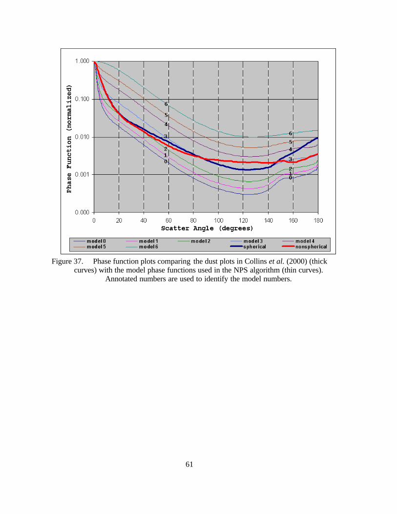
61
Figure 37. Phase function plots comparing the dust plots in Collins et al. (2000) (thick
curves) with the model phase functions used in the NPS algorithm (thin curves). Annotated numbers are used to identify the model numbers.

62
THIS PAGE INTENTIONALLY LEFT BLANK
63
VI. CONCLUSIONS AND RECOMMENDATIONS
A. CONCLUSIONS
A radiative transfer algorithm (NPS algorithm) that processes AOD within a
cloud-free maritime atmosphere was presented for the NOAA POES AVHRR and GOES
imager. This algorithm applies linearized, single-scatter theory with an estimate of bi-
directional surface reflectance. Using a technique developed by Durkee et al. (1991),
scattering phase functions are parameterized to seven aerosol size distributions by
applying the ratios of channel 1 and 2 radiances (S12) of the AVHRR. The S12 value is
then translated to an aerosol model index (AMI) value that is accessed by GOES
processing. Both the NOAA and GOES processing then apply the AMI to a look up table
to determine the scattering phase function. The development and validation of the NPS
algorithm is a continuation of the initial work performed by Brown (1997).
Unlike the AVHRR data, the GOES-8 visible radiance data required an
unconventional calibration scheme developed by Rao et al. (1999) and Rao and Zhang
(1999). During the analysis period of this paper (July and August, 2001) signal gain
factors ranging from 1.727 during the first case study (July 27, 2001) through 1.740
during the last study (September 25, 2001) were applied to the GOES raw channel 1
albedo data. In addition, preliminary comparisons of AOD between GOES and NOAA,
and AERONET revealed that an additional GOES-8 channel 1 correction factor of
–5.5Wm-2 sr-1µm-1 was necessary.
To validate the NPS algorithm, retrieved AOD data was collected from 22 cases
during July and September of 2001 and compared to AERONET radiometers positioned
within 3 island locations of the western Atlantic Ocean. For each case, a time series
format was used to study temporal variations in AOD. Overall, the comparison dataset
has a correlation coefficient of 0.67 with a standard error of 0.07. Within higher AOD
cases (da > 2.5), the general trend was for the NPS-generated AOD values to under-
estimate AERONET-observed conditions, probably due to assumptions of non-absorption
applied to aerosol particles. When related to scatter angles, the NPS-generated AOD
64
calculations performed best within the backscatter angle ranges of 130o - 140o and 170o -
180o.
A major part of the uncertainty to the AOD processing is the proper selection of
the scattering phase function. The problem with the AOD results generated from GOES
data is that the aerosol conditions over a particular region were assumed to be unchanging
throughout the entire time period, which might last for 8 hours. Unfortunately, trying to
validate a representative aerosol dis tribution was beyond the scope of this study. The
AOD results were apparently not very sensitive to any aerosol model assigned to the
calculation.
The pattern of the NPS algorithm-generated phase functions was evaluated during
the dust events (da = 0.25). Between the scatter angles of 140o through 180o, the phase
function pattern required to match AERONET observations indicated a flatter profile
than that produced by the NPS algorithm on GOES and NOAA data. The AERONET-
generated phase function profile was confirmed with studies by Collins et al. (2000) for
non-spherical dust aerosols compared to spherical particles assumed in the NPS
algorithm.
B. RECOMMENDATIONS
Several research initiatives would aid in the improvement of the NPS algorithm:
• Coordinate with aerosol modelers to develop a more accurate assessment of aerosol conditions on a global scale. The NAAPS model developed at NRL is one such source. The NAAPs would greatly help the NPS algorithm in determining the proper phase function parameters.
• Apply the NPS algorithm to other satellite platforms. Preliminary studies by Brown (2001) indicate that the SeaWiFs sensor, with its suite of visible sensing channels, could greatly enhance the S12 phase function parameterization technique. Another instrument with great potential applications is the Moderate Resolution Imaging Spectroradiometer (MODIS).
• Improve sun glint removal process by incorporating wind speed, which is available from the Defense Meteorological Satellite Program’s (DMSP) Special Sensor Microwave/Imager (SSM/I) data as well as from a variety of regional and global numerical models such as COAMPSTM and NOGAPS.
65
• Develop an on-board calibration to the GOES channel 1 sensors that will greatly reduce AOD uncertainties.
• Refine the phase function lookup table to include more realistic aerosol size distributions for dust events.
• Apply appropriate single-scatter albedo (? o) values for conditions with known absorption properties.

66
THIS PAGE INTENTIONALLY LEFT BLANK
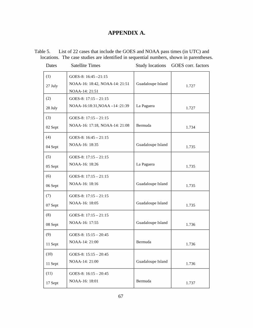
67
APPENDIX A.
Table 5. List of 22 cases that include the GOES and NOAA pass times (in UTC) and locations. The case studies are identified in sequential numbers, shown in parentheses.
Dates Satellite Times Study locations GOES corr. factors
(1)
27 July
GOES-8: 16:45 –21:15
NOAA-16: 18:42, NOAA-14: 21:51
NOAA-14: 21:51
Guadaloupe Island
1.727
(2)
28 July
GOES-8: 17:15 – 21:15
NOAA-16:18:31,NOAA –14 :21:39
La Paguera
1.727
(3)
02 Sept
GOES-8: 17:15 – 21:15
NOAA-16: 17:18, NOAA-14: 21:08
Bermuda
1.734
(4)
04 Sept
GOES-8: 16:45 – 21:15
NOAA-16: 18:35
Guadaloupe Island
1.735
(5)
05 Sept
GOES-8: 17:15 – 21:15
NOAA-16: 18:26
La Paguera
1.735
(6)
06 Sept
GOES-8: 17:15 – 21:15
NOAA-16: 18:16
Guadaloupe Island
1.735
(7)
07 Sept
GOES-8: 17:15 – 21:15
NOAA-16: 18:05
Guadaloupe Island
1.735
(8)
08 Sept
GOES-8: 17:15 – 21:15
NOAA-16: 17:55
Guadaloupe Island
1.736
(9)
11 Sept
GOES-8: 15:15 – 20:45
NOAA-14: 21:00
Bermuda
1.736
(10)
11 Sept
GOES-8: 15:15 – 20:45
NOAA-14: 21:00
Guadaloupe Island
1.736
(11)
17 Sept
GOES-8: 16:15 – 20:45
NOAA-16: 18:01
Bermuda
1.737
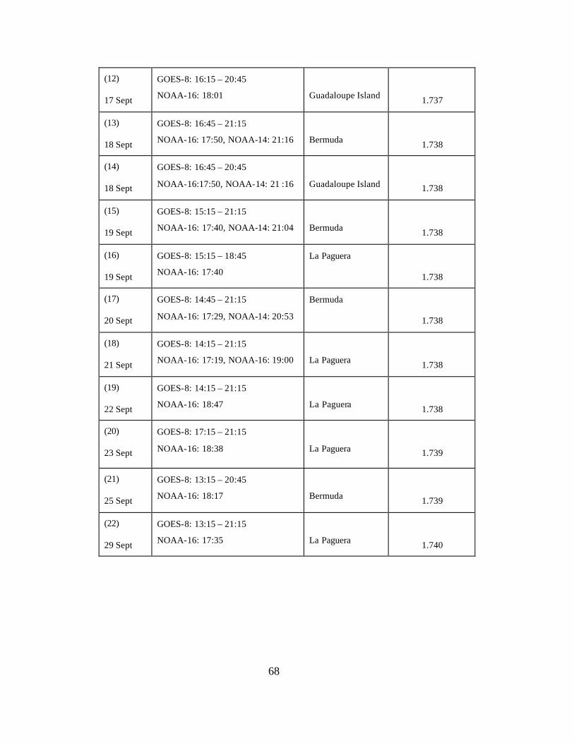
68
(12)
17 Sept
GOES-8: 16:15 – 20:45
NOAA-16: 18:01
Guadaloupe Island
1.737
(13)
18 Sept
GOES-8: 16:45 – 21:15
NOAA-16: 17:50, NOAA-14: 21:16
Bermuda
1.738
(14)
18 Sept
GOES-8: 16:45 – 20:45
NOAA-16:17:50, NOAA-14: 21 :16
Guadaloupe Island
1.738
(15)
19 Sept
GOES-8: 15:15 – 21:15
NOAA-16: 17:40, NOAA-14: 21:04
Bermuda
1.738
(16)
19 Sept
GOES-8: 15:15 – 18:45
NOAA-16: 17:40
La Paguera
1.738
(17)
20 Sept
GOES-8: 14:45 – 21:15
NOAA-16: 17:29, NOAA-14: 20:53
Bermuda
1.738
(18)
21 Sept
GOES-8: 14:15 – 21:15
NOAA-16: 17:19, NOAA-16: 19:00
La Paguera
1.738
(19)
22 Sept
GOES-8: 14:15 – 21:15
NOAA-16: 18:47
La Paguera
1.738
(20)
23 Sept
GOES-8: 17:15 – 21:15
NOAA-16: 18:38
La Paguera
1.739
(21)
25 Sept
GOES-8: 13:15 – 20:45
NOAA-16: 18:17
Bermuda
1.739
(22)
29 Sept
GOES-8: 13:15 – 21:15
NOAA-16: 17:35
La Paguera
1.740
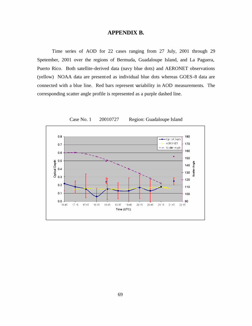
69
APPENDIX B.
Time series of AOD for 22 cases ranging from 27 July, 2001 through 29
Spetember, 2001 over the regions of Bermuda, Guadaloupe Island, and La Paguera,
Puerto Rico. Both satellite-derived data (navy blue dots) and AERONET observations
(yellow) NOAA data are present ed as individual blue dots whereas GOES-8 data are
connected with a blue line. Red bars represent variability in AOD measurements. The
corresponding scatter angle profile is represented as a purple dashed line.
Case No. 1 20010727 Region: Guadaloupe Island
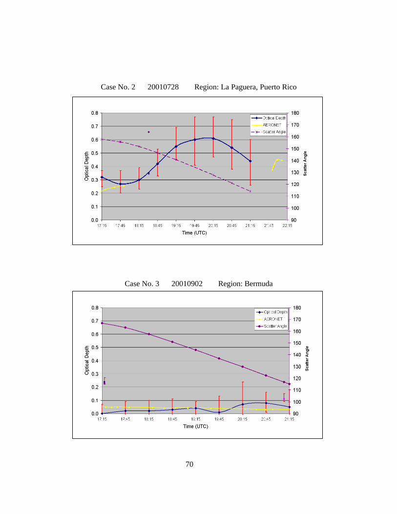
70
Case No. 2 20010728 Region: La Paguera, Puerto Rico
Case No. 3 20010902 Region: Bermuda

71
Case No. 4 20010904 Region: Guadaloupe Island
Case No. 5 20010905 Region: La Paguera, Puerto Rico
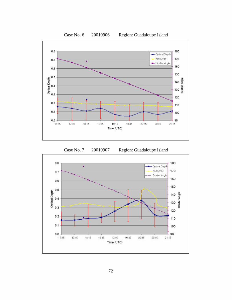
72
Case No. 6 20010906 Region: Guadaloupe Island
Case No. 7 20010907 Region: Guadaloupe Island

73
Case No. 8 20010908 Region: Guadaloupe Island
Case No. 9 20010911 Region: Bermuda

74
Case No. 10 20010911 Region: Guadaloupe Island
Case No. 11 20010917 Region: Bermuda
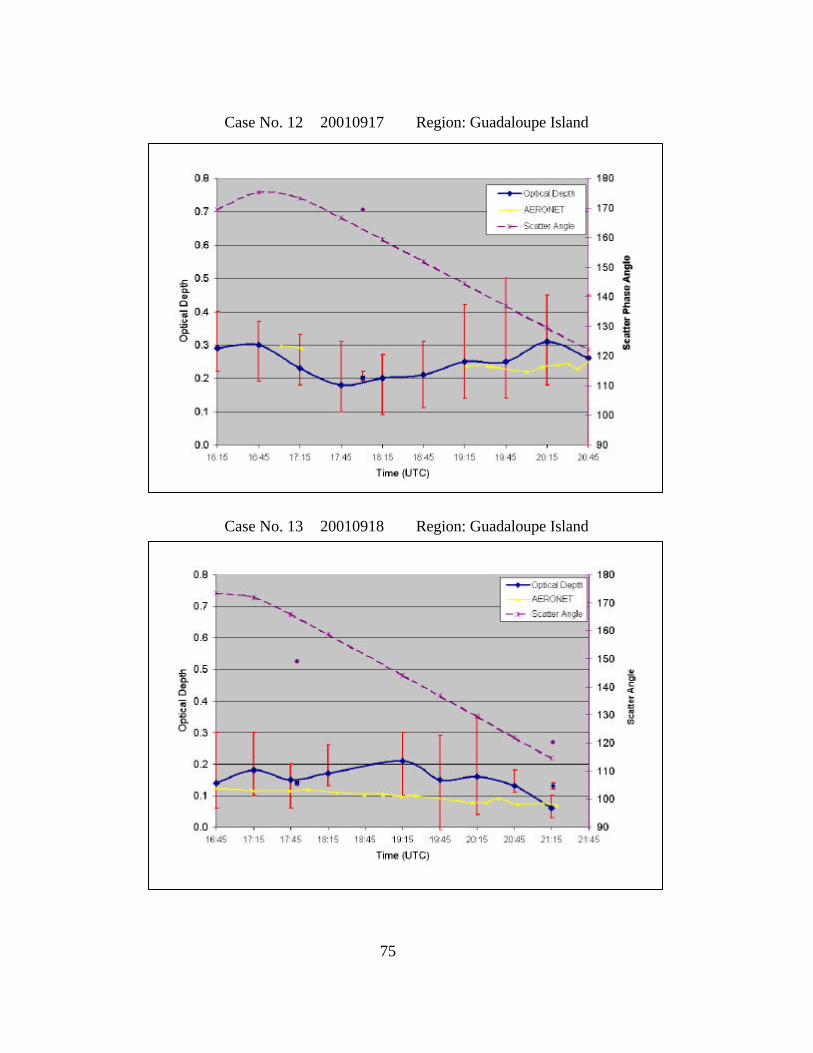
75
Case No. 12 20010917 Region: Guadaloupe Island
Case No. 13 20010918 Region: Guadaloupe Island

76
Case No. 14 20010918 Region: Guadaloupe Island
Case No. 15 20010919 Region: Bermuda

77
Case No. 16 20010919 Region: La Paguera, Puerto Rico
Case No. 17 20010920 Region: Bermuda
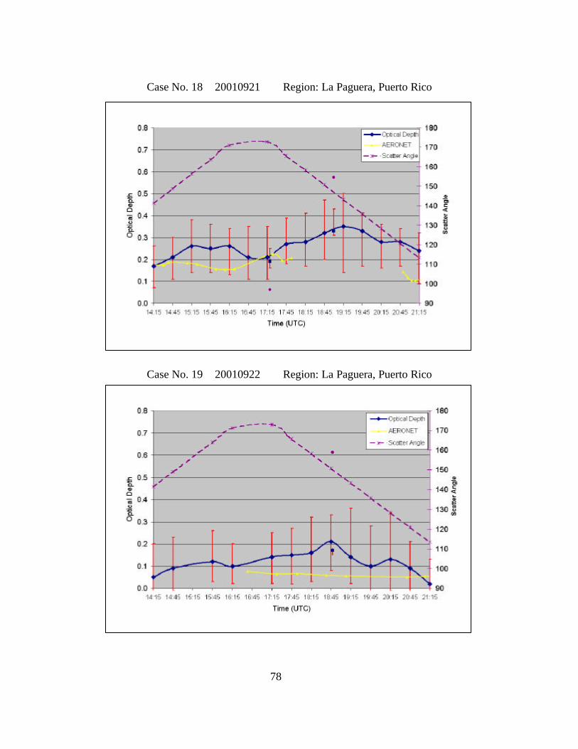
78
Case No. 18 20010921 Region: La Paguera, Puerto Rico
Case No. 19 20010922 Region: La Paguera, Puerto Rico
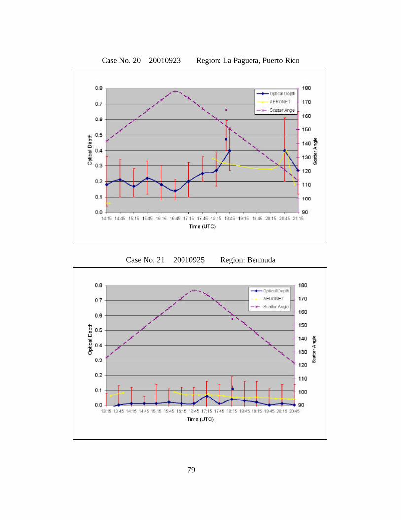
79
Case No. 20 20010923 Region: La Paguera, Puerto Rico
Case No. 21 20010925 Region: Bermuda

80
Case No. 22 20010929 Region: La Paguera, Puerto Rico
81
LIST OF REFERENCES
Bloembergen , N., C. K. Patel and G. Pake (chairpersons), 1987: Science and technology of directed energy weapons. Report of the American Physical Society Study Group, Reviews of Modern Physics, 59, S1-S202. Brown, B. B., 1997: Remote measurement of aerosol optical properties using the NOAA POES AVHRR and GOES Imager during TARFOX. M.S. Thesis, Naval Postgraduate School, Monterey, CA, 73 pp. Brown, B. A., 2001: Aerosol optical depth retrieval by NPS Model modified for SeaWiFS input. M.S. Thesis, Naval Postgraduate School, Monterey, CA, 61 pp. Charlson, R. J., S. E. Swartz, J. M. Hales, R. D. Cess, J. A. Coakley, Jr., J. E. Hansen and D. J. Hoffman, 1992: Climate forcing by anthropogenic aerosols. Science, 255, 423-430. Collins, D. R., H. H. Jonsson, J. H. Seinfeld, R. C. Flagan, S. Gassó, D. A. Hegg, P. B. Russell, B. Schmid, J. M. Livingston, E. Öström, K. J. Noone, L. M. Russell and J. P. Putaud, 2000: In situ aerosol –size distributions and clear-column radiative closure during ACE-2. Tellus, 52B, 498-525. Cordray, D. M., J. W. Fitzgerald, S. G. Gathman, J. N. Hayes, J. E. Kenney, G. P. Mueller and R. E. Ruskin (1977). Meteorological sensitivity study on high energy laser propagation. Naval Research Laboratory Report 8097, Washington, D.C. 81pp. Cox, C. and W. Munk, 1954: Measurement of the roughness of the sea surface from photographs of the sun’s glitter. Journal of the optical Society of America., 44, 838-850. Durkee, P. A., F. Pfeil, E. Frost, and R. Shema, 1991: Global analysis of aerosol particle characteristics. Atmos. Env., 25A, 2457-2471. Durkee, P. A., K. E. Nielsen, P. J. Smith, P. B. Russell, B. Schmid, J. M. Livingston, B. N. Holben, C. Tomasi, V. Vitale, D. Collins, R. C. Flagan, J. H. Seinfeld, K. J. Noone, E. Öström, S. Gasso, D. Hegg, L. M. Russell, T. S. Bates and P. K. Quinn, 1999: Regional aerosol optical depth characteristics from satellite observations: ACE-1, TARFOX and ACE-2 results. Tellus, 51B, 1-14. Higurashi, A. and T. Nakajima, 1999: Development of a two channel aerosol retrieval algorithm on global scale using NOAA/AVHRR. J. Atmos. Sci., 56, 924-941. Higurashi, A. T., T. Nakajima, B. N. Holben, A. Smirnov, R. Frouin, and B. Chateret, 1999: A study of global aerosol optical climatology with two channel AVHRR remote sensing. J. Climate, 13, 2011-2027.
82
Holben, B. N., T. F. Eck, I. Slutsker, D. Tanré, J. P. Buis, A. Setzer, E. Vermote, J. A. Reagan, Y. J. Kaufman, T. Nakajima, F. Lavenu, I. Jankowiak, and A. Smirnov, 1998: AERONET – A federated instrument network and data archive for aerosol characterization. Remote Sens. Environ., 66, 1-16. Intergovernmental Panel on Climate Change (IPCC), 1996. Climate Change 1995, J. T. Houghton et al. (Eds.). Cambridge University Press, New York. Kaufman, Y. J., R. S. Fraser, and R. A. Ferrare, 1990: Satellite measurements of large-scale air pollution methods. J. Geophys. Res., 95, 9895-9909. King, M. D., Y. J. Kaufman, D. Tanré, and T. Nakajima, 1999: Remote sensing of tropospheric aerosols from space: past, present and future. Bull. Am. Meteor. Soc., 80, 2229-2259. Liou, K. N., 1980: An Introduction to Atmospheric Radiation. Academic Press, New York, 393pp. Rao, C. R. N. and N. Zhang, 1999: Calibration of the visible channel of the GOES images using the Advanced Very High Resolution Radiometer. Pre-print volume, 10th Atmospheric Radiation Conference (Madison, Wisconsin), 560-563. Rao, C. R. N., C. J. Sullivan, and N. Zhang, 1999: Post-launch calibration of meterorlogical satellite sensors. Adv Space Res., 23, 1357-1365. Smith, P. J., 1998: Remote measurement of aerosol optical properties using the NOAA POES AVHRR during ACE-1, TARFOX, and ACE-2. M.S. Thesis, Naval Postgraduate School, Monterey, CA, 58 pp. Twomey, S., M. Piepgrass and T. L. Wolfe, 1977: An assessment of the impact of pollution on global cloud albedo. Tellus, 36B, 356-366. Westphal, D. L., 2002: Overview of NAAPS: Navy Aerosol Analysis and Prediction System. http://www.nrlmry.navy.mil/aerosol/Docs/nlrmryonrprop.html.

83
INITIAL DISTRIBUTION LIST
1. Defense Technical Information Center Ft. Belvoir, Virginia
2. Dudley Knox Library Naval Postgraduate School Monterey, California
3. CDR James A. Hill Naval Postgraduate School Monterey, California
4. Chairperson, Department of Meteorology Naval Postgraduate School Monterey, California
5. Professor Philip A. Durkee, MR/De Naval Postgraduate School Monterey, California
6. Superintendent, Naval Research Laboratory, Code 7500 Monterey, California
7. Dr. Ted L. Tsui, Code 7540 Naval Research Laboratory Monterey, California
8. Dr. Douglas L. Westphal, Code 7533
Naval Research Laboratory Monterey, California
9. Mr. Jeffrey D. Hawkins, Code 7541 Naval Research Laboratory Monterey, California
10. Dr. Jeffrey S. Reid
SPAWAR San Diego, California
11. Dr. Sundar A. Christopher
University of Alabama Huntsville, Alabama