aerodynamics and noise of coaxial jets

1550 AIAA JOURNAL VOL. 15, NO. 11

Aerodynamics and Noise of Coaxial Jets

Thomas F. Balsa*General Electric Research and Development Center, Schenectady, N. Y.

andPhilip R. Gliebet

General Electric Aircraft Engine Group, Evendale, Ohio

The objective of this investigation was to develop a unified prediction method for estimating theaerodynamic and noise characteristics of jets issuing from nozzles of arbitrary geometric shapes. The methodhas been developed and demonstrated for dual-flow coaxial jets. An extension of Reichardt's theory is utilized topredict the mean velocity, temperature, and axial turbulence intensity distributions throughout the jet plume.The generic noise intensity spectrum is synthesized by a "slice-of-jet" approach, wherein each axial location inthe plume contributes to the sound generation in one dominant frequency band. The propagation of the sourcespectrum to the far field is modeled by means of convected quadrupoles embedded in a parallel slug flow. Ex-tensive predictions of the aeroacoustic characteristics of coaxial jets were made and compared with experiment.The agreement between theory and experiment is quite good, except at high frequencies and shallow angles to thejet axis, where refraction is overestimated. A major conclusion drawn from these results is that the noisereduction attained by a coaxial jet conies primarily from a reduction in turbulence intensity.

NomenclatureAj = jet nozzle cross-sectional areaa — jet nozzle inner stream exit radiusOjj = azimuthal average of (/, j) quadrupole

amplitudeb = jet nozzle outer stream exit radiusbm - mixing layer momentum thicknessbh = mixing layer enthalpy thicknessCm = momentum spreading rate parameterCh = enthalpy spreading rate parameterCi>c2>co = speed of sound in inner, outer, and ambient

regions, respectivelycp - specific heat at constant pressureD - jet nozzle effective diameter/ = observed frequencyH - local stagnation enthalpy relative to ambientH(

n1} = Hankel function of the first kind, order n

Jn = Bessel function of the first kind, order nKlfK2fK0 = propagation constant in inner, outer, and

ambient regions, respectivelyk] = wave number u/c0I = typical turbulent correlation length scaleMc = source convection Mach number Us fc0p = acoustic pressureQij =(i, j) quadrupoleR = distance from nozzle exit to observerr = radial coordinate5 = jet plume cross-sectional area at distance xSt - source Strouhal number /(I —Mc cos6)a/UIJT = jet temperatureT0 = ambient temperature/ = timeU/,U2 = velocity in inner and outer streamsUs = source convection velocity

Received July 14, 1976; presented as Paper 76-492 at the 3rd AIAAAero-Acoustics Conference, Palo Alto, Calif., July 20-23, 1976;revision received May 31,1977.

Index categories: Aeroacoustics; Jets, Wakes, and Viscid-InviscidFlow Interactions.

*Engineer, Applied Mechanics Branch, Power Generation andPropulsion Laboratory.

tSenior Engineer, Theoretical Aerocoustics, Advanced Engineeringand Technology Programs Department.

u = axial (x) component of velocityv = radial (r) component of velocityx = axial coordinateYn = Bessel function of the second kind, order ny,z = transverse coordinates in x = constant planeA = Laplacian operator<5 = delta function<t> = angle between elemental shear stress vector

and radial coordinatea. = angular coordinate of elemental jet0 = azimuthal coordinate angle9 = angle between jet axis (x coordinate) and

observerp = fluid densitya = radial coordinate of elemental jetr = turbulent Reynolds stressa? = radian source frequencyVR = nozzle exit velocity ratio (U2/U,)jAR = nozzle exit area ratio (b2 — a2)/a^TR = nozzle exit temperature ratio (c2/c1 ) jSPL = !/3-octave band sound pressure level, re:

2 x 10 ~ 4 dynes/cm2

OASPL = overall sound pressure level, re: 2 x l O ~ 4

dynes/cm2

Superscripts and Subscripts

= statistical time average= differentiation or fluctuating component= complex conjugate= Fourier transform= value at nozzle exit plane

( ) j = value in inner stream or region( ) 2 = value in outer stream or region< > = statistical time average

Introduction

IN the past few years, considerable progress has been madein achieving an understanding of the noise produced by hot

and cold round jets. This progress is a direct result of carefuland accurate jet noise measurements1"4 and new theoreticaldevelopments.5'7 The latter have focused on one importantaspect of jet noise, namely acoustic/mean-flow interaction.

Dow

nloa

ded

by A

nado

lu U

nive

rsity

on

Apr

il 29

, 201

4 | h

ttp://

arc.

aiaa

.org

| D

OI:

10.

2514

/3.6

0822

NOVEMBER 1977 AERODYNAMICS AND NOISE OF COAXIAL JETS 1551

It was recognized that a successful jet noise predictionmethod must include the modeling of both noise generationand propagation. The former is intimately tied to turbulence,an area not understood well quantitatively. Experimentalturbulence data relevant to jet noise are somewhat limited,8"12

but it appears that, through various similarity arguments, it ispossible to predict the turbulence characteristics of round jetsquite well. Similarly, the propagation aspects of round jetnoise have been treated satisfactorily. Perhaps the mostcomplete treatment is given by Mani,6 who found that the jetmean flow has a profound effect on the far-field noisedirectivity over the entire frequency spectrum. At highfrequencies refraction effects become important, as was firstdemonstrated by Atvars et al.13 At low frequencies additional(above Lighthill-Ribner theory) convective amplificationeffects appear.

It was desirable to extend these turbulence and acousticmodels to other nozzle configurations. The primarymotivation was to develop a tool to study the parametricdependence of noise on nozzle shape. Such a tool would beindispensable in the search for a *'quiet" nozzle. A secondaryobjective was to check the generality of the conceptsdeveloped to describe round nozzle jet noise.

In this article, a model of the aeroacoustic characteristics ofcoplanar, coaxial nozzles is developed. This is the simplestextension of the round jet work. Considerable acoustic dataexist for this geometry, and comparisons of predictions withexperiment are presented for a wide range of inner-to-outerstream velocity ratios and exhaust area ratios. The measuredfeatures of coaxial jet noise are predicted quite well.

Prediction Model: General RemarksThe development of the present prediction method rests on

two primary assumptions: 1) the dominant jet noisegeneration mechanism is the random momentum fluctuationsof the small-scale turbulent structure in the mixing regions ofthe jet plume; and 2) the propagation of this noise to the far-field observer is altered significantly by the surrounding jetflow in which the turbulent eddies are embedded and con-vecting. Therefore it is proposed that the jet produces anintrinsic noise intensity spectrum directly relatable to thestatistical aerodynamic properties of the jet (i.e., meanvelocity and density distributions, and local turbulentstructure properties such as length-scale, intensity) which ismodified by acoustic/mean-flow interactions.

The prediction method follows a sequence of three basicsteps: 1) prediction of the aerodynamic characteristics (meanvelocity, density, and turbulent structure properties); 2)evaluation of the turbulent mixing noise at 90 deg to the jetaxis utilizing the flow properties from 1 and the Lighthill-Ribner theory; and 3) construction of the far-field soundspectrum at various observer positions, utilizing the results of1 and 2, and accounting for the source convection andacoustic/mean-flow interaction using Lilley's equation.

Jet Plume AerodynamicsAs was discussed in the previous section, an aerodynamic

prediction of the jet plume is required to provide the strengthof the noise sources. The method selected is an extension ofReichardt's theory,14 which basically synthesizes the complexflows from nozzles of arbitrary geometry by superposition ofa suitable distribution of elemental round jet flows. Thisapproach was first suggested by Alexander et al.15 and ap-plied directly to suppressor nozzle configurations by Lee etal.16 and Grose and Kendal.17

Reichardt's theory is a semiempirical one, based on ex-tensive experimental observations that the axial momentumflux profiles were bell-shaped or Gaussian in the fullydeveloped similarity region (suitably far downstream) of a jet.From this observation, a hypothesis for the relation betweenaxial and transverse momentum flux was formulated whichyields a governing equation for the axial momentum flux. For

the far downstream similarity region of a round jet withnozzle area Aj and exit velocity Uj the governing equation andsolution are as follows:

d_~dx{

d / ar or

A,

where

(pu2y=Pju2-^-e-^b^2

\ = l/2 bmdbm/dx

(1)

(2)

(3)

and bm (x) is the axial momentum mixing region width, takento be proportional to the axial distance x from the nozzle exitplane,

bm(x)=Cmx (4)

The jet spreading rate Cm becomes a key parameter in thetheory, and is determined experimentally. The coordinatesystem is shown in Fig. 1.

Because Eq. (1) is linear, the summation of elementalsolutions, Eq. (2), is also a solution. This unique feature ofReichardt's theory allows the construction of quite complexjet flows with relatively simple mathematics. Although morerigorous (but containing just as much empiricism, albeit indifferent forms) theories are available for simple (round andplane) jets, there is no other technique available which offersthe capability for modeling jet flows typical of aircraft enginesuppressor nozzles such as multitube, lobe, and chute nozzles,etc.

Consider a distribution of elemental jets issuing parallel tothe x axis, whose exit areas lie in the x = Q plane. Eachelemental jet has an exit area Aj= o do da, located at (a, a,0), as shown in Fig. 1. The axial momentum flux at adownstream point (r, 6, x) due to the elemental jet exhaustingat (or, a, 0) is given by Eq. (2)

d(pu2y=PjU2((jd(jda/irb2m)e-(t/bni)2 (5)

where

£2 = r2 +a2 -2ra cos(0-a)

Integrating Eq. (5), the following solution is obtained:

<pu2y(r,e,x) = ~l-r\\(pjUl)e-tt'b'n)2adada (6)

From the distribution of (pjUj) in the exit plane, the localvalue of (pu2 > at any point (r, 6, x) can be found from Eq.(6) by standard numerical integration. Assuming that the jetplume stagnation enthalpy flux //diffuses in the same manneras axial momentum, and analogous expression for stagnationenthalpy flux (puffy can be derived,

(puffy(r,d,x) = ~ (7)

where bh is the thermal shear layer width, taken to beproportional to x

bh = Chx, Ch = constant (8)

The stagnation enthalpy is defined as H=cpT+ l/2U2 —cpT0,and the thermal layer spreading rate Ch also must be obtainedexperimentally. Assuming that the jet mixing occurs atconstant static pressure equal to the ambient value, thesolutions for (pu2} and <pw//> given by Eqs. (6) and (7) aresufficient to determine the distributions of mean axial velocityu and temperature /"throughout the jet plume.

Dow

nloa

ded

by A

nado

lu U

nive

rsity

on

Apr

il 29

, 201

4 | h

ttp://

arc.

aiaa

.org

| D

OI:

10.

2514

/3.6

0822

1552 T. F. BALSA AND P. R. GLIEBE AIAA JOURNAL

axisymmetric nozzles, T = rr, and re =0. This will be the casefor the coaxial jet problem discussed in later sections, but themore general formulation is presented for completeness. Thebasic limiting assumptions made were: 1) the jet plume mixingoccurs at constant static pressure, equal to the ambient value,and 2) the flow is primarily axial with all nozzle exit elementsin the same plane x - 0.

Noise Intensity Spectrum at 90 degThe aerodynamic characteristics of the jet plume provide

the information required to evaluate the acoustic intensityspectrum at 90 deg to the jet axis using the Lighthill-Ribnertheory of jet noise. This basic spectrum provides a goodestimate of the far-field noise spectrum at 90 deg to the jetaxis since sound/flow interaction effects are minimal there.Then the noise at any other point in the far field can becomputed from this result and the directivity pattern derivedin the following section. The analysis presented in thefollowing parallels the work of Lighthill,18 Ribner,19

Lilley,20 and Powell21; especially the work of the latter three,as it relates to the use of various similarity arguments.

The far-field mean-square sound pressure, in absence ofsound/flow interaction effects is given by18'19

Fig. 1 Jet flow coordinate system and nomenclature: a) nozzle exitplane, b) plume in (r,x) plane, c) nomenclature for elemental jet at((7,a,0) and field point P.

In addition to the jet plume mean flow properties, theturbulent Reynolds stress, assumed to be proportional to thetransverse momentum flux, also can be obtained. Reichardt'shypothesis [from which Eq. (1) evolved] states that thetransverse momentum flux is proportional to the transversegradient of the axial momentum flux, the proportionalityfactor being \(x). For a simple round jet, from Eqs. (2-4),the Reynolds stress r is given by

-xrdr(9)

For an elemental jet exhausting at (a, a, 0) the shear stress Tat (r, 6, x) lies along a line connecting (a, a, 0) and theprojection of (r, 6,x) onto the x = 0 plane. This vector is at anangle <t> to the coordinate direction r (Fig. 1). The radialcomponent of the shear stress dr at point (r, 6, x) due to anelemental jet exhausting at (a, a, 0) is then dr^^dr cos<£.Similarly, the azimuthal component is dre=dr sin</>. Per-forming the same summation and limiting process over allelemental jets, the total shear stress at (r, 6, x) is then foundto be

(10)

where

Tr{r,B,x) = -%- \ \pjU2(£/bm)e-(t/b>r>)2cos<}> a da da (11)irb m J J

and Te(r,B,x) is given by a similar expression with cos</>replaced by sin0. The distance £ is again given by the ex-pression following Eq. (6), and the angle 0 is given by

= r — a cos(0 — a) (12)

Equations (5-12) provide the basic expressions for com-putation of the jet plume flow parameters T, ii, and r for anozzle of arbitrary exit cross section and exit distribution ofvelocity and temperature.f It may be noted that, for

where (pv/Uj) is the fluid momentum flux ( i j ) componentevaluated at vector position^' and time / ' , and ( p v k v t ) is the(k,l) component evaluated at y" and t". The retarded times/ ' and t" are given by (t — R'/c0) and (t — R"/c0),respectively. Note that v-t and x, denote the / components ofvelocity and source-to-observer distance R, respectively.Defining separation vectors and time delay rj=yf — y" andT=t'—t", respectively, and an eddy coordinatey= y2 (yf +y"), the foregoing expression may be written inthe following form

n d4

-~4((pvivJ)(pvivl)yd3rid3y (13)

where A:7 =R cos0, x2=R sinB cos0, andx3 =R sinO sin0.In order to evaluate Eq. (13), some assumptions about the

turbulent structure must be made. Because of the lack ofdetailed experimental or theoretical information ap-proximations are made, following the pioneering work ofRibner,19 Lilley,20 and Powell.21

The derivatives with respect to T are assumed to beequivalent to multiplying by a typical turbulent eddy fluc-tuation frequency w relative to the moving eddy, and theintegral over the separation is equivalent to multiplication byI3, where / is the eddy length scale. Thus,

X ;X ;

JThe quantities (pu2 > and (puH} are interpreted as pit2 and puH.

Since the aerodynamic model described in the previoussection provides radial and azimuthal distributions of flowproperties u, T, re, and rr at successive axial stations x, it isconvenient to express the volume integration in Eq. (14) asd3y = d S ( x ) dx, where S(x) is the cross-sectional area of theplume. The summation over all components (/, j) of thefluctuating momentum stress tensor in Eq. (14) yields oneterm that is omnidirectional (self-noise) and another term

Dow

nloa

ded

by A

nado

lu U

nive

rsity

on

Apr

il 29

, 201

4 | h

ttp://

arc.

aiaa

.org

| D

OI:

10.

2514

/3.6

0822


having a basic directivity of (cos^0 + cos20). The latter iscalled shear noise; see, for example, the work of Ribner.22

Confining ourselves to 0 = 90 deg for the moment, andreferring to </?2> at 0 = 90 deg as the intrinsic or basic noisespectrum, it is now assumed that (pv^j} in Eq. (14) is ap-proximately represented by the turbulent shear stress r. Inaddition, the typical frequency co is assumed to be related to u,p, and r by the equation

and that(15a)

(15b)

These assumed relationships, derived from similarityarguments by Lee et al.,16 are consistent with the ex-perimental measurements of Davies et al.8 The basic or in-trinsic acoustic pressure level is then as follows, after com-bining Eqs. (14) and (15):

1 { (T2c4

0R2 J JP2u(r/p)7/2dS(x)— (16)

Equations (15) imply that the typical eddy fluctuationfrequency at any axial location x is given by

(17)

In practice, it was found that, through model calibrationswith low-velocity round jet data, Eq. (17) should be modifiedas follows:

= 10(x/D) (18)

where UM is taken to be the maximum mean velocity at a givencross section. From Eqs. (16) and (18), the source spectrumcan be computed through the approximation, as suggested byPowell,21

d77d/

dx dd/

Note that D is a characteristic length scale of the jet nozzle.For a round jet, D is simply the nozzle diameter. For a coaxialjet, D will be defined in a later section. Substituting Eqs. (16)and (18) into the foregoing expression, the following equationfor the far-field intrinsic spectrum at 0 = 90 deg results:

16d/// \ X ^M 4 V1

2 4r>2 ^~~A — ~~ Tit2ciR2 L UM dx 3 J

x j p2w(T /p) 7 / 2dSU) (19)

To summarize the results of this section, the intrinsic noisespectrum in the absence of convection and refraction effectsat 0 = 90 deg is obtained from numerical evaluation of Eq.(19). This expression involves an integration, over the jetplume cross section, of a suitable source strength[ p 2 w ( r / p ) 7 / 2], comprised of flow parameters p, «, and r,which are evaluated from the extended Reichardt modeldiscussed in the previous section. In the following section, thesound/flow interaction modeling approach developed sosuccessfully for simple round jets by Mani6 will be applied tothe coaxial jet problem. This will provide the directionalcharacteristics of the sound sources in the jet flow as a func-tion of flow variables and frequency. By combining thepreviously generated noise spectrum calculation with thesound/flow interaction prediction model, the net absolutesound spectrum at any observer angle 0 in the far field canthen be estimated.

A similar theoretical development was reported by Chen23

for coaxial jets which employed Reichardt 's theory for the

aerodynamic prediction and the slice-of-jet concepts21 forpower spectrum prediction. Only power spectrum was con-sidered, and both convection and refraction were ignored.Since power spectrum is the result of integrating soundpressure spectra over a suitably distant sphere in the far field,it can be expected that neglect of sound/flow interactioneffects will give incorrect power level estimates at all but thelowest jet velocities.

The Noise DirectivityThe previous sections have described how the basic noise

intensity is calculated from the turbulence properties of thejet. The noise generated by turbulence in the jet can bemodeled as a distribution of convecting sources radiating tothe far field at a specific frequency. The objective of thissection is to evaluate how a convecting noise source of givenstrength and frequency radiates to the far field. This radiationpattern differs considerably from the classical result ofLighthill1 8 because, in the present formulation, the source issurrounded by a rapidly moving hot jet. The analyticaldevelopment follows very closely the work of Mani6; adetailed discussion of the implications of the simplifyingassumptions made herein can be found in that work.

Our starting point is Lilley's equation,24 which, in the caseof a slug flow velocity profile, simplifies to the followingequation for acoustic pressure/?:

~^ + U^J P-c2*P=S(x-Ust)S(r-r())d(8-80)-—

(20)

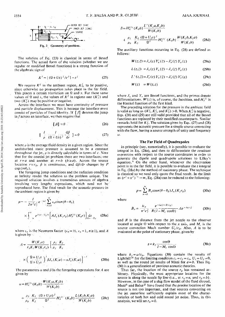
The jet plume, for the purpose of evaluating the acousticpropagation effects, is modeled as two coaxial slug flow jets,as shown in Fig. 2. A convecting source is located within slugflow at r()<a and 80. The source moves at velocity Us in thedownstream direction while emitting sound at frequency co inits own (convecting) reference frame. The slug flow velocity Uand speed of sound c take on values of £//, U2, U0, and c,, c2,c() in each of the three regions (inner flow, outer flow, andambient), respectively. Note that U, is some representativeaverage value of inner stream velocity, not necessarily equalto nozzle exit value; the same remark holds for U2 in the outerstream.

The solution to Eq. (20), satisfying suitable jump con-ditions across the fluid interfaces at r — a and r = b, andobeying the Sommerfeld radiation condition at r=oo, isobtained by Fourier transforms. Define the Fourier transformof p as

=—( f27T« ) - ° ° J - °

peinee-*l'e-ixxdBdtdx

whose inverse is

p = ——A { £4ltZ J -oo J -oo ~_

(21)

(22)

and apply the transformation (21) to Eq. (20). After a numberof integrations by parts (and ignoring the contributions fromupper and lower limits), we find

d2p J dp r(n^rr«\2

T^7 +

- eineo

dr2

where

Here, 12, s, and n are the Fourier transform variables.

(23)

(24)

Dow

nloa

ded

by A

nado

lu U

nive

rsity

on

Apr

il 29

, 201

4 | h

ttp://

arc.

aiaa

.org

| D

OI:

10.

2514

/3.6

0822

1554 T.'F. BALSA AND P. R. GLIEBE AIAA JOURNAL

n .0, cnU

./—" // 1

OUTER JET (FAN)- INNER JET (CORE)

SOURCE

r ^ *Fig. 2 Geometry of problem.

The solution of Eq. (23) is classical in terms of Besselfunctions. The actual form of the solution (whether we useregular or modified Bessel functions) is a strong function ofthe algebraic sign of

(25)

We require K2 in the ambient region, K20> to be positive,

since otherwise no propagation takes place in the far field.This places a certain restriction on Q and s. For these samevalues of Q and 5, the values of K2 in regions one (K2) andtwo (K2

2) may be positive or negative.Across the interfaces we must have continuity of pressure

and particle displacement. This is because the interface mustconsist of particles of fixed identity. If [/fl denotes the jumpin/across an interface, we then require that

1 dp. p (Q + Us)2 dr

(26)

(27)

where p is the average fluid density in a given region. Since theundisturbed static pressure is assumed to be a constantthroughout the jet, p is directly calculable in terms of c. Notethat for the coaxial jet problem there are two interfaces; oneat r — a and another at r = b (b>a). Across the sourcelocation r — r0, p is continuous, and dp/dr changes by F

The foregoing jump conditions and the radiation conditionat infinity render the solution to the problem unique. Therequired solution involves a tremendous amount of algebrainvolving very lengthy expressions, which need not bereproduced here. The final result for the acoustic pressure inthe ambient region is given by

P=~1

(28a)

where £„ is the Neumann factor (t0= '/i, - e » = 1, «>1), and Ais given by

WKi") \ Pi K2r0K-iW(K,r0) L p, K,

(28b)

The parameters a and (3 in the foregoing expressions for A aregiven by

„ ^W(K2a,K2b)W(K2b)

P2 K0

Po

L'(K2a,K2b)1 W(K2b)

The auxiliary functions occurring in Eq. (28) are defined asfollows:

,& =Jn (z) Y'n ( f ) - J l ( f ) Yn (z)

'n ( f ) ~J'n ( f ) Y'n

W(z) =

(29a)

(29b)

(29c)

(29d)

where Jn and Yn are Bessel functions, and the primes denotedifferentiations. W(z) is, of course, the Jacobian, and H(

n1} is

the Hankel function of the first kind.The preceding solution for the pressure in the ambient field

is valid as long as ( K ] , K22, and K2

0) > 0. When K2/ is negative,Eqs. (28) and (29) are still valid provided that all of the Besselfunctions are replaced by their modified counterparts. Similarremarks hold for K2

2. The solution given by Eqs. (27) and (28)represents the acoustic pressure for a simple source convectingwith the flow, having a source strength of unity and frequency

The Far Field of QuadrupolesIn principle (say, numerically), it is possible to evaluate the

integral in Eq. (28a), and then to differentiate the resultantexpression with respect to the source coordinates in order togenerate the dipole and quadrupole solutions to Lilley'sequation.6 On the other hand, whenever the observationpoint is in the far field, it is possible to evaluate the s integralin Eq. (28a) by the method of stationary phase. The techniqueis classical so we need only quote the final result. In the limitas (r2 + x2) ^ — oo, Eq. (28a) can be reduced to the following:

p=

wheree-iu(t-R/c0)

T2c2t /?(7-Mccos0) -Ae

(30a)

(30b)

and R is the distance from the jet nozzle to the observerlocated at angle 0 with respect to the x axis, and Mc is thesource convection Mach number Us/c0. Also, A is to beevaluated at the point of stationary phase, given by

cosB7-Mc cos0

(30c)

where k]=u/c0. Equations (30) contain the results ofLighthill18 for the limiting condition c; =c2 =c0, U} = U2=0,as well as the round jet results of Mani for a = b. Thus Eq.(30) is a generalization of previous acoustic theories.

Thus far, the location of the source r0 has remained ar-bitrary. Physically, the most appropriate location for thesource is along the nozzle lip line (i.e., at r0 = a, and r0 = b).However, in the case of a slug flow model of the fluid shroud,Mani6 and Balsa25 have found that the precise location of thesource is not too important, and that sources convecting onthe jet centerline sufficiently explain most of the charac-teristics of both hot and cold round jet noise. Thus, in thisanalysis, we will set r0 = 0.

Dow

nloa

ded

by A

nado

lu U

nive

rsity

on

Apr

il 29

, 201

4 | h

ttp://

arc.

aiaa

.org

| D

OI:

10.

2514

/3.6

0822


Equation (30a) is now expanded in a Taylor series aboutr0 = 0, yielding the result

9C7 sm6+(y20-z2

0)C2 cos20

K2i(y2o + z2o)C0 + 0(r30) (31a)+ 2y0z0C2 s

whereBn \K] \ n'2

(31b)

and (y0, z0) denote the transverse coordinates of the source.The upper sign in Eq. (3 la) is used when K] >0, whereas thelower sign is used when K]<Q, and T ( n ) is the Gammafunction.

The transverse dipole and quadrupole solutions can beobtained from Eq. (3 la) by differentiating with respect to y0and z0 and then setting r0 = 0. Also, differentiations withrespect to x generate longitudinal dipole and quadrupolesolutions. This latter operation is equivalent to multiplicationby s given by Eq. (30c); symbolically, d/dx-^s.

As an example, consider the y— y quadrupole Q22 — QyrThe solution in terms of the simple source solution is given byEq.(31a),

r <*2p i= Qyy=\ -j-r = 2C2 cos28 =F UK] C0 (32)

L oy 0 J r = 0

The square of the amplitude of this quadrupole is given by

where Q* is the complex conjugate of Q. If we define, for anyquadrupole (/,./),

we find that

(33)

(34)

Physically, a22 is the azimuthal average of the amplitude of aring of totally incoherent y—y quadrupoles.

The expression for acoustic pressure, Eq. (3la), is valid fora "unit" convecting (and compact) velocity fluctuation. Bothin the Lilley and Lighthill formulations, the strength of thenoise source is proportional to the jet density. Mani6 hasshown that a compact velocity quadrupole in a heated jetgenerates dipole and source terms. A detailed derivation ofthese terms is omitted herein for brevity, but the final ex-pressions are quoted in the following:

cos'0

_ _ 2a'2=~4k'

(1-MC cos0)4

cos20

(35a)

; / dp \(35b)

(35c)

(35d)

In these equations, (p, dp/dr, d 2 p / d r 2 ) are some represen-tative values of the density and its various gradients. Theexact computation of these gradients follows the proceduresproposed by Mani.6 Note that, when p = 1, Eq. (35c) reducesto Eq. (34), as required.

Finally, there remains to combine these quadrupoles so thatthe noise source is effectively an eddy of isotropic turbulence,as suggested by Ribner.22 In the present terminology, theapproximate mean square pressure is given by

p2 - (an+4a12+2a22 +2a23) (36)

The factor of proportionality in Eq. (36) is directly relatableto the turbulence properties^ in the jet supplied by theaerodynamic calculation. If p2 is known at one angle (say 6= 90 deg), this factor can be found and Eq. (36) can be used tofind the mean square pressure at all other angles. Byevaluating Eq. (36) at.0 = 90...deg and equating to Ihe ex-pression given by Eq. (19), the constant of proportionality canbe evaluated. Thus, the absolute level and directivity in eachfrequency band can be estimated.

Discussion of ResultsIn applying the previously described model to coplanar jet

noise predictions, three further assumptions had to be made.First, it was found, through examination of flowfieldmeasurements, that the jet momentum spreading parameterCm varies with outer-to-inner stream velocity ratio as follows:

(37)

and Um[n and £/max are thewhere CmQ «0.075, and Ch «C,minimum and maximum values of (U"lt U2) evaluated at thenozzle exit. This relationship is independent of nozzle arearatio, and reflects the reduction in mixing rate when thestreams on both sides of the mixing zone are moving in thesame direction. The second assumption made concerns theselection of a diameter of characteristic, length D to use indetermining the typical frequency of each jet slice, as given byEq. (18). A suitable expression for D which satisfies thelimiting conditions when U2 - 0 or U} = U2 is

a + (b-a) (38)

A final assumption made was that the "suitable average"values of Uj and U2 used in evaluation of the directivity

110

90

1AR =

>^

AR -

*SS

0

2.1

""-

3.9

1 ^

.2

i.

4

i/

Y

6

7

/y

8

80

110

i- c

AR

k^

AR =

^^^

))

= 9.3

^

43.5

x^

2

*^

co/

f -4

(

V

//6

^y

f/

8 1

Fig. 3 Overall SPL at 9 = 90 deg as a function of area and velocityratios.' Cold jet, U/j - 980 f ps (o Olsen's data, —— present theory).

Dow

nloa

ded

by A

nado

lu U

nive

rsity

on

Apr

il 29

, 201

4 | h

ttp://

arc.

aiaa

.org

| D

OI:

10.

2514

/3.6

0822


90

SPL

80

SPL

80

SPL

80

.2 .4

° n 0

^

Fig. 4 SPL at 0 = 90 degas a function ofvelocity ratio. AR = 3.9. Cold jet,£/ /y=980 fps (o Olsen's data, ——present theory).

.2 .4

90

SPL

on

80(

SPI

(

70

VR =

^

VR =

o^^

VR =

fn

0.8

^ 3 \

0.6

0.5

rtf*^

,noj

f O w (

ui <

i o o j^- -^

^ o o J**. _ _

> O n~*-— — "S

louJ

> o o o

L-Q^)0

0 ry

^

•^Oj

• n t

Fig. 5 SPL at 0 = 90 deg as a function ofvelocity ratio. AR = 9.3. Cold jet,<7 /y=980 fps (o Olsen's data, ——present theory).

Freq. kHz Freq. kHz

0 20 40 61

20 40 60 80 100 0 120

0 20 40 60 80 100 Q 120

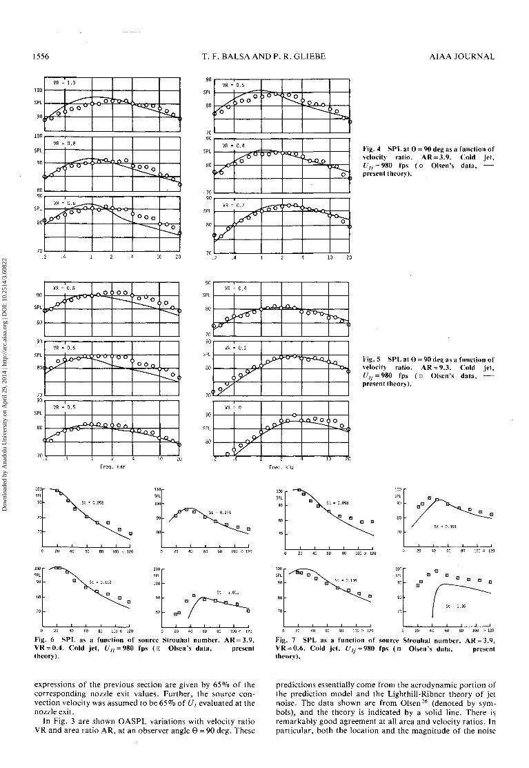
Fig. 6 SPL as a function of source Strouhal number. AR = 3.9,VR = 0.4. Cold jet, £/ /y=980 fps (0 Olsen's data, —— presenttheory).

0 20 40 60

0 20 40 60 80 100 0 120

0 20 40 60 80 100 0 120

0 20 40 60

Fig. 7 SPL as a function of source Strouhal number. AR = 3.9,VR = 0.6. Cold jet, £/ /y=980 fps ( B Olsen's data, —— presenttheory).

expressions of the previous section are given by 65% of thecorresponding nozzle exit values. Further, the source con-vection velocity was assumed to be 65% of U, evaluated at thenozzle exit.

In Fig. 3 are shown OASPL variations with velocity ratioVR and area ratio AR, at an observer angle 6 = 90 deg. These

predictions essentially come from the aerodynamic portion ofthe prediction model and the Lighthill-Ribner theory of jetnoise. The data shown are from Olsen26 (denoted by sym-bols), and the theory is indicated by a solid line. There isremarkably good agreement at all area and velocity ratios. Inparticular, both the location and the magnitude of the noise

Dow

nloa

ded

by A

nado

lu U

nive

rsity

on

Apr

il 29

, 201

4 | h

ttp://

arc.

aiaa

.org

| D

OI:

10.

2514

/3.6

0822


0 20 40 60 80 100 0 1200 20 40 60

0 20 40 60 80 100 0 120 0 20 40 60 80 100 6 120

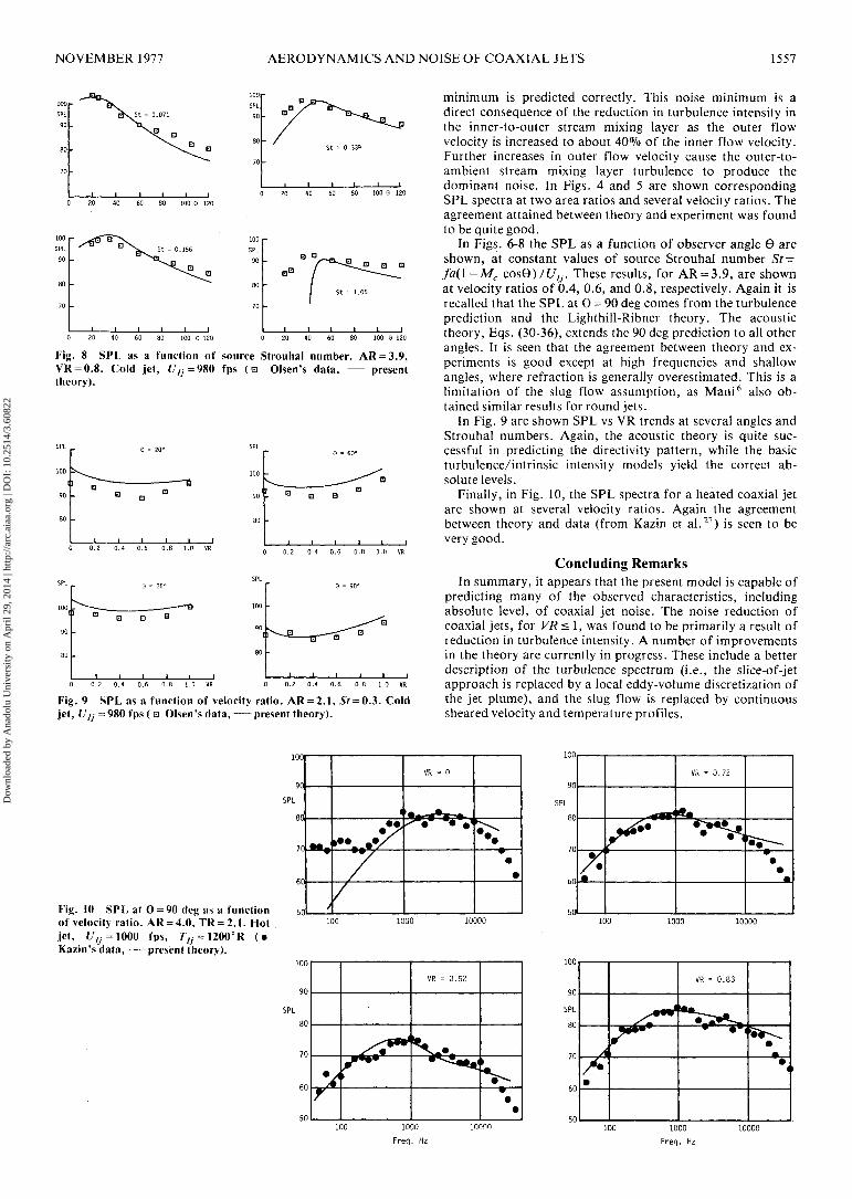
Fig. 8 SPL as a function of source Strouhal number. AR = 3.9,VR = 0.8. Cold jet, £/ /y=980 fps ( m Olsen's data, —— presenttheory).

0.2 0.4 0.6 0.8 1.0 VR 0 0.2 0.4 0.6 0.8 1.0 VR

0 0.2 0.4 0.6 0.8 1.0 VR 0 0.2 0.4 0.6 0.8 1.0 VR

Fig. 9 SPL as a function of velocity ratio. AR = 2.1, SY = 0.3. Coldjet, Uij = 980 fps ( B Olsen's data, —— present theory).

minimum is predicted correctly. This noise minimum is adirect consequence of the reduction in turbulence intensity inthe inner-to-outer stream mixing layer as the outer flowvelocity is increased to about 40% of the inner flow velocity.Further increases in outer flow velocity cause the outer-to-ambient stream mixing layer turbulence to produce thedominant noise. In Figs. 4 and 5 are shown correspondingSPL spectra at two area ratios and several velocity ratios. Theagreement attained between theory and experiment was foundto be quite good.

In Figs. 6-8 the SPL as a function of observer angle 9 areshown, at constant values of source Strouhal number St =fa(\ -Mc cos0)/(7/y. These results, for AR = 3.9, are shownat velocity ratios of 0.4, 0.6, and 0.8, respectively. Again it isrecalled that the SPL at 9 = 90 deg comes from the turbulenceprediction and the Lighthill-Ribner theory. The acoustictheory, Eqs. (30-36), extends the 90 deg prediction to all otherangles. It is seen that the agreement between theory and ex-periments is good except at high frequencies and shallowangles, where refraction is generally overestimated. This is alimitation of the slug flow assumption, as Mani6 also ob-tained similar results for round jets.

In Fig. 9 are shown SPL vs VR trends at several angles andStrouhal numbers. Again, the acoustic theory is quite suc-cessful in predicting the directivity pattern, while the basicturbulence/intrinsic intensity models yield the correct ab-solute levels.

Finally, in Fig. 10, the SPL spectra for a heated coaxial jetare shown at several velocity ratios. Again the agreementbetween theory and data (from Kazin et al.27) is seen to bevery good.

Concluding RemarksIn summary, it appears that the present model is capable of

predicting many of the observed characteristics, includingabsolute level, of coaxial jet noise. The noise reduction ofcoaxial jets, for VR < 1, was found to be primarily a result ofreduction in turbulence intensity. A number of improvementsin the theory are currently in progress. These include a betterdescription of the turbulence spectrum (i.e., the slice-of-jetapproach is replaced by a local eddy-volume discretization ofthe jet plume), and the slug flow is replaced by continuoussheared velocity and temperature profiles.

Fig. 10 SPL at 0 = 90 deg as a functionof velocity ratio. AR = 4.0, TR = 2.1. Hotjet, (7^ = 1000 fps, 7/7 = 1200°R (•Kazin's data, —— present theory).

100

1000 10000

1000 10000Freq. Hz

Dow

nloa

ded

by A

nado

lu U

nive

rsity

on

Apr

il 29

, 201

4 | h

ttp://

arc.

aiaa

.org

| D

OI:

10.

2514

/3.6

0822


AcknowledgmentThe authors are grateful to R. Mani of General Electric

Corporate Research and Development and E.J. Stringas ofGeneral Electric Aircraft Engine Business Group for theirencouragement, patience, and technical help. We also wish tothank W. Olsen of NASA Lewis Research Center forproviding a complete set of data.

References'Lush, P.A., "Measurements of Subsonic Jet Noise and Com-

parison with Theory," Journal of Fluid Mechanics, Vol. 46, 1971, pp.477-500.

2Ahuja, K.K. and Bushell, K.W., "An Experimental Study ofSubsonic Jet Noise and Comparison with Theory," Journal of Soundand Vibration, Vol. 30, 1973, pp. 317-341.

3Cocking, B.J., "The Effect of Temperature on Subsonic JetNoise," National Gas Turbine Establishment Rept. No. 331, 1974.

4Tanna, H.K. and Dean, P.O., "The Influence of Temperature onShock-Free Supersonic Jet Noise," Journal of Sound and Vibration,Vol.39, 1975, pp. 429-460.

5Tester, B.J. and Burrin, R.H., "On Sound Radiation fromSources in Parallel Sheared Jet Flows," AIAA Paper 74-57, Jan.1974.

6 Mani, R., "The Influence of Jet Flow on Jet Noise-Part 1 andPart 2," Journal of Fluid Mechanics, Vol. 73, 1976, pp. 753-793.

7 Balsa, T.F., "Fluid Shielding of Low Frequency ConvectedSources by Arbitrary Jets," Journal of Fluid Mechanics, Vol. 70,1975. pp. 17-36.

8Davies, P.O.A.L., Fisher, M.J. , and Barratt, M.J., "TheCharacteristics of the Turbulence in the Mixing Region of a RoundJet," Journal of Fluid Mechanics, Vol. 15, 1963, pp. 337-367.

9Davies, P.O.A.L., "Turbulence Structure in Free Shear Layers,"AIAA Journal, Vol. 4, Nov. 1966, pp. 1971-1978.

1()Davies, P.O.A.L., "Structure of Turbulence," Journal of Soundand Vibration, Vol. 28, 1973, pp. 513-526.

"Davis, M.R., "Intensity, Scale and Convection of TurbulentDensity Fluctuations," Journal of Fluid Mechanics, Vol. 70, 1975,pp. 463-479.

1 2Chu, Wing T., "Turbulence Measurements Relevant to JetNoise," University of Toronto, UTIAS Rept. No. 119, 1966.

13Atvars, J., Schubert, L.K., Grande, E., and Ribner, H.S.,"Refraction of Sound by Jet Flow and Temperature," NASA CR494,1966.

14Schlichting, H., Boundary Layer Theory, 4th ed., McGraw-Hill,New York, 1960.

15Alexander, L.G., Baron, T., and Comings, W., "Transport ofMomentum, Mass and Heat in Turbulent Jets," University of Illinois,Engineering Experiment Station Bull. No. 413, May 1953.

16Lee, R., Kendall, R., et al., "Research Investigation of theGeneration and Suppression of Jet Noise," General Electric, CRNOas 59-6160-C, ASTIA No. AD-251887, 1961.

17Grose, R.D. and Kendall, R.M., "Theoretical Predictions of theSound Produced by Jets Having an Arbitrary Cross Section," ASMESymposium on Fully Separated Flows, May 1964.

1 8Lighthi l l , M.J., "On Sound Generated Aerodynamically I.General Theory," Proceedings of the Royal Society of London, Vol.A211, 1952, pp. 564-587.

19Ribner, H.S., "On the Strength Distribution of Noise SourcesAlong a Jet," University of Toronto, UTIAS Rept. No. 51, 1958.

20Lilley, G.M., "On the Noise from Air Jets," AeronauticalResearch Council (London), Rept. 20, 376; P.M. 2724, 1958.

21Powell, A., "Similarity and Turbulent Jet Noise," Journal of theAcoustical Society of America, Vol. 31, 1959, pp. 812-813.

22Ribner, H.S., "Quadrupole Correlations Governing the Patternof Jet Noise," Journal of Fluid Mechanics, Vol. 38, 1969, pp. 1-24.

23Chen, C.Y., "A Model for Predicting Aeroacoustic Charac-teristics of Coaxial Jets," AIAA Paper 76-4, 1976.

24Lilley, G.M., "The Generation and Radiation of Supersonic JetNoise," Vol. IV, Air Force Aero-Propulsion Laboratory, TR-72-53,1972.

25 Balsa, T.F., "The Shielding of a Convected Source by an An-nular Jet with Application to the Performance of Multitube Sup-pressors," Journal of Sound and Vibration, Vol. 44, 1976, pp. 179-189.

26Olsen, W. and Friedman, R., "Jet Noise from Coaxial NozzlesOver a Wide Range of Geometric and Flow Parameters," AIAAPaper 74-43, 1974.

27Kazin, S.B., et al., "Core Engine Noise Control Program,"General Electric Company Contractor Final Rept. No. FAA-RD-74-125,1974.

Dow

nloa

ded

by A

nado

lu U

nive

rsity

on

Apr

il 29

, 201

4 | h

ttp://

arc.

aiaa

.org

| D

OI:

10.

2514

/3.6

0822

aerodynamics and noise of coaxial jets

Documents