NBER WORKING PAPER SERIES

ADVANCES IN CONSUMPTION-BASED ASSET PRICING:EMPIRICAL TESTS

Sydney C. Ludvigson

Working Paper 16810http://www.nber.org/papers/w16810

NATIONAL BUREAU OF ECONOMIC RESEARCH1050 Massachusetts Avenue

Cambridge, MA 02138February 2011

Forthcoming in Volume 2 of the Handbook of the Economics of Finance, edited by George Constantinides,Milton Harris and Rene Stulz. I am grateful to Timothy Cogley, Martin Lettau, Abraham Lioui, HannoLustig, Stephan Nagel, Monika Piazzesi, Stijn Van Nieuwerburgh, Laura Veldkamp, Annette Vissing-Jorgensen, and to the editors for helpful comments, and to Peter Gross and David Kohn for excellentresearch assistance. The views expressed herein are those of the author and do not necessarily reflectthe views of the National Bureau of Economic Research.

NBER working papers are circulated for discussion and comment purposes. They have not been peer-reviewed or been subject to the review by the NBER Board of Directors that accompanies officialNBER publications.

© 2011 by Sydney C. Ludvigson. All rights reserved. Short sections of text, not to exceed two paragraphs,may be quoted without explicit permission provided that full credit, including © notice, is given tothe source.

Advances in Consumption-Based Asset Pricing: Empirical TestsSydney C. LudvigsonNBER Working Paper No. 16810February 2011, Revised April 2011JEL No. E21,G1,G12

ABSTRACT

The last 15 years has brought forth an explosion of research on consumption-based asset pricing asa leading contender for explaining aggregate stock market behavior. This research has propelled furtherinterest in consumption-based asset pricing, as well as some debate. This chapter surveys the growingbody of empirical work that evaluates today's leading consumption-based asset pricing theories usingformal estimation, hypothesis testing, and model comparison. In addition to summarizing the findingsand debate, the analysis seeks to provide an accessible description of a few key econometric methodologiesfor evaluating consumption-based models, with an emphasis on method-of-moments estimators. Finally,the chapter offers a prescription for future econometric work by calling for greater emphasis on methodologiesthat facilitate the comparison of multiple competing models, all of which are potentially misspecified,while calling for reduced emphasis on individual hypothesis tests of whether a single model is specifiedwithout error.

Sydney C. LudvigsonDepartment of EconomicsNew York University19 W. 4th Street, 6th FloorNew York, NY 10002and NBERsydney.ludvigson@nyu.edu

1 Introduction

The last 15 years has brought forth an explosion of research on consumption-based asset

pricing as a leading contender for explaining aggregate stock market behavior. The explo-

sion itself represents a dramatic turn-around from the intellectual climate of years prior, in

which the perceived failure of the canonical consumption-based model to account for almost

any observed aspect of financial market outcomes was established doctrine among finan-

cial economists. Indeed, early empirical studies found that the model was both formally

and informally rejected in a variety of empirical settings.1 These findings propelled a wide-

spread belief (summarized, for example, by Campbell (2003) and Cochrane (2005)) that the

canonical consumption-based model had serious limitations as a viable model of risk.

Initial empirical investigations of the canonical consumption-based paradigm focused

on the representative agent formulation of the model with time-separable power utility. I

will refer to this formulation as the “standard” consumption-based model hereafter. The

standard model has difficulty explaining a number of asset pricing phenomena, including the

high ratio of equity premium to the standard deviation of stock returns simultaneously with

stable aggregate consumption growth, the high level and volatility of the stock market, the

low and comparatively stable interest rates, the cross-sectional variation in expected portfolio

returns, and the predictability of excess stock market returns over medium to long-horizons.2

In response to these findings, researchers have altered the standard consumption-based

model to account for new preference orderings based on habits or recursive utility, or new

restrictions on the dynamics of cash-flow fundamentals, or new market structures based

on heterogeneity, incomplete markets, or limited stock market participation. The habit-

formation model of Campbell and Cochrane (1999), building on work by Abel (1990) and

Constantinides (1990), showed that high stock market volatility and predictability could be

explained by a small amount of aggregate consumption volatility if it were amplified by time-

varying risk aversion. Constantinides and Duffie (1996) showed that the same outcomes could

1The consumption-based model has been rejected on U.S. data in its representative agent formulation with

time-separable power utility (Hansen and Singleton 1982, 1983; Ferson and Constantinides, 1991; Hansen

and Jagannathan, 1991; Kocherlakota, 1996); it has performed no better and often worse than the simple

static-CAPM in explaining the cross-sectional pattern of asset returns (Mankiw and Shapiro, 1986; Breeden,

Gibbons, and Litzenberger, 1989; Campbell, 1996; Cochrane, 1996; Hodrick, Ng and Sengmueller, 1998);

and it has been generally replaced as an explanation for systematic risk by financial return-based models

(for example, Fama and French, 1993).2For summaries of these findings, including the predictability evidence and surrounding debate, see Lettau

and Ludvigson (2001b), Campbell (2003), Cochrane (2005), Cochrane (2008), and Lettau and Ludvigson

(2010).

1

arise from the interactions of heterogeneous agents who cannot insure against idiosyncratic

income fluctuations. Epstein and Zin (1989) and Weil (1989) showed that recursive utility

specifications, by breaking the tight link between the coefficient of relative risk aversion and

the inverse of the elasticity of intertemporal substitution (EIS), could resolve the puzzle

of low real interest rates simultaneously with a high equity premium (the “risk-free rate

puzzle”). Campbell (2003) and Bansal and Yaron (2004) showed that when the Epstein

and Zin (1989) and Weil (1989) recursive utility function is specified so that the coefficient

of relative risk aversion is greater than the inverse of the EIS, a predictable component in

consumption growth can help rationalize a high equity premium with modest risk aversion.

These findings and others have reinvigorated interest in consumption-based asset pricing,

spawning a new generation of leading consumption-based asset pricing theories.

In the first volume of this handbook, published in 2003, John Campbell summarized

the state-of-play in consumption-based asset pricing in a timely and comprehensive essay

(Campbell (2003)). As that essay reveals, the consumption-based theories discussed in the

previous paragraph were initially evaluated on evidence from calibration exercises, in which

a chosen set of moments computed from model-simulated data are informally compared to

those computed from historical data. Although an important first step, a complete assess-

ment of leading consumption-based theories requires moving beyond calibration, to formal

econometric estimation, hypothesis testing, and model comparison. Formal estimation, test-

ing, and model comparison present some significant challenges, to which researchers have

only recently turned.

The objective of this chapter is three-fold. First, it seeks to summarize a growing body

of empirical work, most of it completed since the writing of Volume 1, that evaluates leading

consumption-based asset pricing theories using formal estimation, hypothesis testing, and

model comparison. This research has propelled further interest in consumption-based asset

pricing, as well as some debate. Second, it seeks to provide an accessible description of a few

key methodologies, with an emphasis on method-of-moments type estimators. Third, the

chapter offers a prescription for future econometric work by calling for greater emphasis on

methodologies that facilitate the comparison of competing models, all of which are potentially

misspecified, while calling for reduced emphasis on individual hypothesis tests of whether a

single model is specified without error. Once we acknowledge that all models are abstractions

and therefore by definition misspecified, hypothesis tests of the null of correct specification

against the alternative of incorrect specification are likely to be of limited value in guiding

2

theoretical inquiry toward superior specifications.

Why care about consumption-based models? After all, a large literature in finance is

founded on models of risk that are functions of asset prices themselves. This suggests that

we might bypass consumption data altogether, and instead look directly at asset returns. A

difficulty with this approach is that the true systematic risk factors are macroeconomic in

nature. Asset prices are derived endogenously from these risk factors. In the macroeconomic

models featured here, the risk factors arise endogenously from the intertemporal marginal

rate of substitution over consumption, which itself could be a complicated nonlinear function

of current, future and past consumption, and possibly of the cross-sectional distribution of

consumption, among other variables. From these specifications, we may derive an equilibrium

relation between macroeconomic risk factors and financial returns under the null that the

model is true. But no model that relates returns to other returns can explain asset prices in

terms of primitive economic shocks, however well it may describe asset prices.

The preponderance of evidence surveyed in this chapter suggests that many newer con-

sumption theories provide statistically and economically important insights into the behavior

of asset markets that were not provided by the standard consumption-based model. At the

same time, the body of evidence also suggests that these models are imperfectly specified

and statistical tests are forced to confront macroeconomic data with varying degrees of mea-

surement error. Do these observations imply we should abandon models of risk based on

macroeconomic fundamentals? I will argue here that the answer to this question is ‘no.’ In-

stead, what they call for is a move away from specification tests of perfect fit, toward methods

that permit statistical comparison of the magnitude of misspecification among multiple, com-

peting models, an approach with important origins in the work of Hansen and Jagannathan

(1997). The development of such methodologies is still in its infancy.

This chapter will focus on the pricing of equities using consumption-based models of

systematic risk. It will not cover the vast literature on bond pricing and affine term structure

models. Moreover, it is not possible to study an exhaustive list of all models that fit the

consumption-based description. I limit my analysis to the classes of consumption-based

models discussed above, and to studies with a significant econometric component.

The remainder of this chapter is organized as follows. The next section lays out the

notation used in the chapter and presents background on the consumption-based paradigm

that will be referenced in subsequent sections. Because many estimators currently used

are derived from, or related to, the Generalized Method of Moments (GMM) estimator of

3

Hansen (1982), Section 3 provides a brief review of this theory, discusses a classic GMM asset

pricing application based on Hansen and Singleton (1982), and lays out the basis for using

non-optimal weighting in GMM and related method of moments applications. This section

also presents a new methodology for statistically comparing specification error across mul-

tiple, non-nested models. Section 4 discusses a particularly challenging piece of evidence for

leading consumption-based theories: the mispricing of the standard model. Although lead-

ing theories do better than the standard model in explaining asset return data, they have

difficulty explaining why the standard model fails. The subsequent sections discuss specific

econometric tests of newer theories, including debate about these theories and econometric

results. Section 5 covers scaled consumption-based models. Section 6 covers models with

recursive preferences, including those that incorporate long-run consumption risk and sto-

chastic volatility (Section 7). Section 8 discusses estimation of asset pricing models with

habits. Section 9 discusses empirical tests of asset pricing models with heterogeneous con-

sumers and limited stock market participation. Finally, Section 10 summarizes and concludes

with a brief discussion of models that feature rare consumption disasters.

2 Consumption-BasedModels: Notation and Background

Throughout the chapter lower case letters are used to denote log variables, e.g., let denote

the level of consumption; then log consumption is ln () ≡ . Denote by the price of

an equity asset at date , and let denote its dividend payment at date I will assume,

as a matter of convention, that this dividend is paid just before the date- price is recorded;

hence is taken to be the -dividend price. Alternatively, is the end-of-period price.

The simple return at date is denoted

< ≡ +

−1− 1

The continuously compounded return or log return, , is defined to be the natural logarithm

of its gross return:

≡ log (1 +<)

I will also use +1 denote the gross return on an asset from to + 1,

≡ 1 +<

4

Vectors are denoted in bold, e.g., R denotes a × 1 vector of returns {}=1 Consumption-based asset pricing models imply that, although expected returns can vary

across time and assets, expected discounted returns should always be the same for every

asset, equal to 1:

1 = (+1+1) (1)

where +1 is any traded asset return indexed by . The stochastic variable +1 for which

(1) holds will be referred to interchangeably as either the stochastic discount factor (SDF),

or pricing kernel. +1 is the same for each asset. Individual assets display heterogeneity in

their risk adjustments because they have different covariances with the stochastic variable

+1.

The moment restriction (1) arises from the first-order condition for optimal consumption

choice with respect to any traded asset return +1, where the pricing kernel takes the form

+1 = (+1+1)(+1)

, given a utility function defined over consumption and possibly other

arguments , and where denotes the partial derivative of with respect to +1 is

therefore equal to the intertemporal marginal rate of substitution (MRS) in consumption

The substance of the asset pricing model rests with the functional form of and its

arguments; these features of the model drive variation in the stochastic discount factor. The

statistical evaluation of various models for comprises much of the discussion of this chapter.

The return on one-period riskless debt, or the risk-free rate <+1, is defined by

1 +<+1 ≡ 1(+1) (2)

is the expectation operator conditional on information available at time . <+1 is the

return on a risk-free asset from period to + 1. <+1 may vary over time, but its value is

known with certainty at date . As a consequence,

1 = (+1(1 +<+1)) = (+1) (1 +<+1)

which implies (2).

Apply the definition of covariance Cov() = ()− () () to (1) to arrive

5

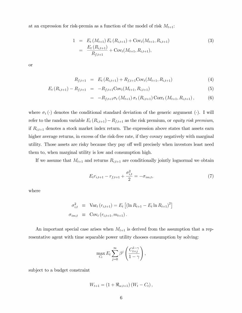
at an expression for risk-premia as a function of the model of risk +1:

1 = (+1) (+1) +Cov(+1 +1) (3)

= (+1)

+1+Cov(+1 +1)

or

+1 = (+1) ++1Cov(+1 +1) (4)

(+1)−+1 = −+1Cov(+1 +1) (5)

= −+1 (+1) (+1)Corr (+1 +1) (6)

where (·) denotes the conditional standard deviation of the generic argument (·). I willrefer to the random variable (+1)−+1 as the risk premium, or equity risk premium,

if +1 denotes a stock market index return. The expression above states that assets earn

higher average returns, in excess of the risk-free rate, if they covary negatively with marginal

utility. Those assets are risky because they pay off well precisely when investors least need

them to, when marginal utility is low and consumption high.

If we assume that +1 and returns +1 are conditionally jointly lognormal we obtain

+1 − +1 +2

2= − (7)

where

2 ≡ Var (+1) =

£(ln+1 − ln+1)

2¤ ≡ Cov (+1+1)

An important special case arises when +1 is derived from the assumption that a rep-

resentative agent with time separable power utility chooses consumption by solving:

max

∞X=0

Ã1−+

1−

!

subject to a budget constraint

+1 = (1 +<+1) ( − )

6

where is the stock of aggregate wealth <+1 is its net return. In this case the pricing

kernel takes the form

+1 =

µ+1

¶−

It is often convenient to use the linear approximation for this model of the stochastic discount

factor:

+1 ≈ [1− ∆ ln+1]

Inserting this approximation into (5), we have

(+1)−+1 = −+1Cov(+1 +1)

=Cov(+1 +1)

Var(+1)

µ−Var (+1)

(+1)

¶=−Cov(∆ ln+1 +1)

Var(∆ ln+1)

µ−

22Var(∆ ln+1)

(+1)

¶=

Cov(∆ ln+1 +1)

Var(∆ ln+1)| {z }≡

µVar(∆ ln+1)

(+1)

¶| {z }

0

(8)

In (8), is the conditional consumption beta, which measures the quantity of consumption

risk. The parameter measures the price of consumption risk, which is the same for all

assets. The asset pricing implications of this model were developed in Rubinstein (1976),

Lucas (1978), Breeden (1979), and Grossman and Shiller (1981). I will refer to the model

(8) as the classic consumption CAPM (capital asset pricing model), or CCAPM for short.

When power utility preferences are combined with a representative agent formulation as in

the original theoretical papers that developed the theory, I will also refer to this model as

the standard consumption-based model.

Unless otherwise stated, hats “b” denote estimated parameters.3 GMM and Consumption-Based Models

In this section I review the Generalized Method of Moments estimator of Hansen (1982) and

discuss its application to estimating and testing the standard consumption based model.

Much of the empirical analysis discussed later in the chapter either directly employs GMM

or uses methodologies related to it. A review of GMMwill help set the stage for the discussion

of these methodologies.

7

3.1 GMM Review (Hansen, 1982)

Consider an economic model that implies a set of population moment restrictions satisfy:

{h (θw)| {z }(×1)

} = 0 (9)

where w is an × 1 vector of variables known at , and θ is an × 1 vector of unknownparameters to be estimated. The idea is to choose θ to make the sample moment as close as

possible to the population moment. Denote the sample moments in any GMM estimation

as g(θ;y ):

g(θ;y )| {z }(×1)

≡ (1 )X=1

h (θw)

where is the sample size, and y ≡¡w0

w0−1 w

01

¢0is a ·× 1 vector of observations.

The GMM estimator bθ minimizes the scalar (θ; yT) = [g(θ; y )]

0(1×)

W(×)

[g(θ; y )](×1)

(10)

where {W}∞=1 a sequence of × positive definite matrices which may be a function of

the data, y .

If = , θ is estimated by setting each g(θ;y ) to zero. GMM refers to the use of (10)

to estimate θ when . The asymptotic properties of this estimator were established by

Hansen (1982). Under the assumption that the data are strictly stationary (and conditional

on other regularity conditions) the GMM estimator bθ is consistent, converges at a rateproportional to the square root of the sample size, and is asymptotically normal.

Hansen (1982) also established the optimal weightingW = S−1, which gives the mini-

mum variance estimator for bθ in the class of GMM estimators. The optimal weighting matrix

is the inverse of

S×=

∞X=−∞

n[h (θw)]

£h¡θw−

¢¤0o

In asset pricing applications, it is often undesirable to useW = S−1. Non-optimal weighting

is discussed in the next section.

The optimal weighting matrix depends on the true parameter values θ. In practice

this means that bS depends on bθ which depends on bS . This simultaneity is typically8

handled by employing an iterative procedure: obtain an initial estimate of θ= bθ(1) , by

minimizing (θ; yT) subject to arbitrary weighting matrix, e.g.,W = I. Use bθ(1) to obtain

initial estimate of S = bS(1) . Re-minimize (θ; yT) using initial estimatebS(1) ; obtain new

estimate bθ(2) . Continue iterating until convergence, or stop after one full iteration. (The two

estimators have the same asymptotic distribution, although their finite sample properties

can differ.) Alternatively, a fixed point can be found.

Hansen (1982) also provides a test of over-identifying (OID) restrictions based on the

test statistic :

≡ ³bθ;y´ ∼ 2( − ) (11)

where the test requires . The OID test is a specification test of the model itself. It tests

whether the moment conditions (9) are as close to zero as they should be at some level of

statistical confidence, if the model is true and the population moment restrictions satisfied.

The statistic is trivial to compute once GMM has been implemented because it is simply

times the GMM objective function evaluated at the estimated parameter values.

3.2 A Classic Asset Pricing Application: Hansen and Singleton

(1982)

A classic application of GMM to a consumption-based asset pricing model is given in

Hansen and Singleton (1982) who use the methodology to estimate and test the standard

consumption-based model. In this model, investors maximize utility

max

" ∞X=0

(+)

#

The utility function is of the power utility form:

() =1−

1− 0

() = ln() = 1

If there are = 1 traded asset returns, the first-order conditions for optimal consump-

tion choice are

− =

©(1 +<+1)

−+1

ª = 1 (12)

9

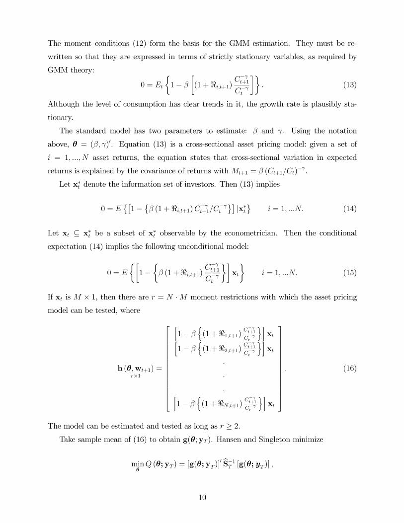
The moment conditions (12) form the basis for the GMM estimation. They must be re-

written so that they are expressed in terms of strictly stationary variables, as required by

GMM theory:

0 =

½1−

∙(1 +<+1)

−+1

−

¸¾ (13)

Although the level of consumption has clear trends in it, the growth rate is plausibly sta-

tionary.

The standard model has two parameters to estimate: and . Using the notation

above, θ = ( )0. Equation (13) is a cross-sectional asset pricing model: given a set of

= 1 asset returns, the equation states that cross-sectional variation in expected

returns is explained by the covariance of returns with +1 = (+1)−.

Let x∗ denote the information set of investors. Then (13) implies

0 = ©£1− © (1 +<+1)

−+1

−

ª¤ |x∗ª = 1 (14)

Let x ⊆ x∗ be a subset of x∗ observable by the econometrician. Then the conditional

expectation (14) implies the following unconditional model:

0 =

½∙1−

½ (1 +<+1)

−+1

−

¾¸x

¾ = 1 (15)

If x is × 1, then there are = · moment restrictions with which the asset pricing

model can be tested, where

h (θw+1)×1

=

⎡⎢⎢⎢⎢⎢⎢⎢⎢⎢⎢⎢⎢⎣

h1−

n(1 +<1+1)

−+1

−

oixh

1− n(1 +<2+1)

−+1

−

oix

···h

1− n(1 +<+1)

−+1

−

oix

⎤⎥⎥⎥⎥⎥⎥⎥⎥⎥⎥⎥⎥⎦ (16)

The model can be estimated and tested as long as ≥ 2.Take sample mean of (16) to obtain g(θ;y ). Hansen and Singleton minimize

min

(θ; y ) = [g(θ; y )]0 bS−1 [g(θ; y )]

10

where bS−1 is an estimate of the optimal weighting matrix, S−1.

Hansen and Singleton use lags of consumption growth and lags of asset returns in x. They

use both a stock market index and industry equity returns as data for <. Consumption is

measured as nondurables and services expenditures from the National Income and Product

Accounts. They find estimates of that are approximately 099 across most specifications.

They also find that the estimated coefficient of relative risk aversion, b is quite low, rangingfrom 035 to 0999. There is no equity premium puzzle here because the model is estimated

using the conditioning information in x. As a consequence, the model is evaluated on a set of

“scaled” returns, or “managed” portfolio equity returnsR+1x. These returns differ from the

simple (unscaled) excess return on stock market that illustrate the equity premium puzzle.

The implications of using conditioning information, or scaling returns, and the importance of

distinguishing between scaled returns and “scaled factors” in the pricing kernel is discussed

in several sections below.

Hansen and Singleton also find that the model is rejected according to the OID test.

Subsequent studies that also used GMM to estimate the standard model find even stronger

rejections whenever both stock returns and a short term interest rate such as a commercial

paper rate are included among the test asset returns, and when a variable such as the price-

dividend ratio is included in the set of instruments x (e.g., Campbell, Lo, and MacKinlay

(1997)). The reason for this is that the standard model cannot explain time variation in the

observed equity risk premium. That is, the model cannot explain the significant forecastable

variation in excess stock market returns over short-term interest rates by variables like the

price-dividend ratio. The moment restrictions implied by the Euler equations state that the

conditional expectation of discounted excess returns must be zero

£+1

+1

¤= 0, where

+1 denotes the return on the stock market index in excess of a short-term interest rate.

Predictability of excess returns implies that the conditional expectation +1 varies. It

follows that a model can only explain this predictable variation if +1 fluctuates in just

the right way, so that even though the conditionally expected value of undiscounted excess

returns varies, its stochastically discounted counterpart

£+1

+1

¤is constant and equal

to zero in all time periods. The GMM results imply that discounted excess returns are still

forecastable when +1 = ³+1

´−, leading to large violations of the estimated Euler

equations and strong rejections of overidentifying restrictions.

In principle, the standard model could explain the observed time-variation in the equity

premium (and forecastability of excess returns by variables such as the price-dividend ratio),

11

given sufficient time-variation in the volatility of consumption growth, or in its correlation

with excess returns. To see this, plug the approximation +1 ≈ [1− ∆ ln+1] into

(6). The GMM methodology allows for the possibility of time-varying moments of ∆ ln+1,

because it is a distribution-free estimation procedure that applies to many strictly stationary

time-series processes, including GARCH, ARCH, stochastic volatility, and others. The OID

rejections are therefore a powerful rejection of the standard model and suggest that a viable

model of risk must be based on a different model of preferences. Findings of this type have

propelled interest in other models of preferences, to which we turn below.

Despite the motivation these findings provided for pursuing newer models of preferences,

explaining the large violations of the standard model’s Euler equations is extremely chal-

lenging, even for leading consumption-based asset pricing theories with more sophisticated

specifications for preferences. This is discussed in Section 4.

3.3 GMM Asset Pricing With Non-Optimal Weighting

3.3.1 Comparing specification error: Hansen and Jagannathan, 1997

GMM asset pricing applications often require a weighting matrix that is different from the

optimal matrix, that is W 6= S−1. One reason is that we cannot use W = S−1 to

assess specification error and compare models. This point was made forcibly by Hansen and

Jagannathan (1997).

Consider two estimated models of the SDF, e.g., the CCAPMwith SDF(1)+1 = (+1)

−,

and the static CAPM of Sharpe (1964) and Lintner (1965) with SDF (2)+1 = + +1,

where +1 is the market return. Suppose that we use GMM with optimal weighting to es-

timate and test each model on the same set of asset returns and, doing so, find that the OID

restrictions are not rejected for (1)+1 but are for

(2)+1 May we conclude that the CCAPM

(1)+1 is superior? No. The reason is that Hansen’s -test statistic (11) depends on the

model-specific matrix. As a consequence, Model 1 can look better simply because the

SDF and pricing errors are more volatile than those of Model 2, not because its pricing

errors are lower and its Euler equations less violated.

Hansen and Jagannathan (1997) (HJ) suggest a solution to this problem: compare models

12

(θ) where θ are parameters of the th SDF model, using the following distance metric:

Dist (θ) ≡qming (θ)

0G−1 g (θ) G ≡ 1

X=1

0| {z }

×

g (θ) ≡ 1

X=1

[(θ)R − 1 ]

The minimization can be achieved with a standard GMM application, except the weighting is

non-optimal withW = G−1 rather thanW = S

−1. The suggested weighting matrix here is

the second moment matrix of test asset returns. Notice that, unlike S−1, this weighting does

not depend on estimates of the model parameters θ, hence the metric Dist is comparable

across models. I will refer to Dist (θ) as the HJ distance.

The HJ distance does not reward SDF volatility. As a result, it is suitable for model

comparison. The HJ distance also provides a measure of model misspecification: it gives

least squares distance between the model’s SDF() and the nearest point to it in space of

all SDFs that price assets correctly. It also gives the maximum pricing error of any portfolio

formed from the assets. These features are the primary appeal of HJ distance. The metric

explicitly recognizes all models as misspecified, and provides method for comparing models

by assessing which is least misspecified. If Model 1 has a lower Dist (θ) than Model 2, we

may conclude that the former has less specification error than the latter.

The approach of Hansen and Jagannathan (1997) for quantifying and comparing speci-

fication error is an important tool for econometric research in asset pricing. Tests of overi-

dentifying restrictions, for example using the test, or other specification tests, are tests of

whether an individual model is literally true, against the alternative that it has any specifi-

cation error. Given the abstractions from reality our models represent, this is a standard any

model is unlikely to meet. Moreover, as we have seen, a failure to reject in a specification

test of a model could arise because the model is poorly estimated and subject to a high

degree of sampling error, not because it explains the return data well. The work of Hansen

and Jagannathan (1997) addresses this dilemma, by explicitly recognizing all models as ap-

proximations. This reasoning calls for greater emphasis in empirical work on methodologies

that facilitate the comparison of competing misspecified models, while reducing emphasis on

individual hypothesis tests of whether a single model is specified without error.

Despite the power of this reasoning, most work remains planted in the tradition of re-

lying primarily on hypothesis tests of whether a single framework is specified without error

13

to evaluate economic models. One possible reason for the continuation of this practice is

that the standard specification tests have well-understood limiting distributions that permit

the researcher to make precise statistical inferences about the validity of the model. A lim-

itation of the Hansen and Jagannathan (1997) approach is that it provides no method for

comparing HJ distances statistically: (1) may be less than (2), but are they statistically

different from one another once we account for sampling error? The next section discusses

one approach to this problem.

3.3.2 Statistical comparison of HJ distance

Chen and Ludvigson (2009) develop a procedure for statistically comparing HJ distances of

competing models using a methodology based on White’s (White (2000)) reality check

approach. An advantage of this approach is that it can be used for the comparison of any

number of multiple competing models of general form, with any stationary law of motion for

the data. Two other recent papers develop methods for comparing HJ distances in special

cases. Wang and Zhang (2003) provide a way to compare HJ distance measures across

models using Bayesian methods, under the assumption that the data follow linear, Gaussian

processes. Kan and Robotti (2008) extend the procedure of Vuong (1989) to compare two

linear SDF models according to the HJ distance. Although useful in particular cases, neither

of these procedures are sufficiently general so as to be broadly applicable. The Wang and

Zhang procedure cannot be employed with distribution-free estimation procedures because

those methodologies leave the law of motion of the data unspecified, requiring only that it

be stationary and ergodic and not restricting to Gaussian processes. The Kan and Robotti

procedure is restricted to the comparison of only two stochastic discount factor models, both

linear. This section describes the method used in Chen and Ludvigson (2009), for comparing

any number of multiple stochastic discount factor models, some or all of them possibly

nonlinear. The methodology does not restrict to linear Gaussian processes but instead

allows for almost any stationary data series including a wide variety of nonlinear time-series

processes such as diffusion models, stochastic volatility, nonlinear ARCH, GARCH, Markov

switching, and many more.

Suppose the researcher seeks to compare the estimated HJ distances of several models.

Let 2 denote the squared HJ distance for model : 2 ≡ (Dist (θ))2. The procedure

can be described in the following steps.

1. Take a benchmark model, e.g., the model with smallest squared HJ distance among

14

= 1 competing models, and denote its square distance 21 :

21 ≡ min{2}=1

2. The null hypothesis is 21 −22 ≤ 0, where 22 is the competing model with the nextsmallest squared distance.

3. Form the test statistic ≡ √ (21 − 22 ).

4. If null is true, the historical value of should not be unusually large, given sampling

error.

5. Given a distribution for , reject the null if its historical value, bT , is greater than

the 95th percentile of the distribution for .

The work involves computing the distribution of which typically has a complicated

limiting distribution. However, it is straightforward to compute the distribution via block

bootstrap (see Chen and Ludvigson (2009)). The justification for the bootstrap rests on the

existence of a multivariate, joint, continuous, limiting distribution for the set {2}=1 underthe null. Proof of the joint limiting distribution of {2}=1 exists for most asset pricingapplications: for parametric models the proof is given in Hansen, Heaton, and Luttmer

(1995). For semiparametric models it is given in Ai and Chen (2007).

This method of model comparison could be used in place of or in addition to hypothesis

tests of whether a single model is specified without error. The method follows the recom-

mendation of Hansen and Jagannathan (1997) that we allow all models to be misspecified

and evaluate them on the basis of the magnitude of their specification error. Unlike their

original work, the procedure discussed here provides a basis for making precise statistical

inference about the relative performance of models. The example here provides a way to

compare HJ distances statistically, but can also be applied to any set of estimated criterion

functions based on non-optimal weighting.

3.3.3 Reasons to Use (and Not to Use) Identity Weighting

Before concluding this section it is useful to note two other reasons for using non-optimal

weighting in GMM or other method of moments approaches, and to discuss the pros and cons

of doing so. Aside frommodel comparison issues, optimal weighting can result in econometric

15

problems in small samples. For example, in samples with large number of asset returns and

a limited time-series component, the researcher may end up with a near singular weighting

matrix S−1 orG−1 . This frequently occurs in asset pricing applications because stock returns

are highly correlated cross-sectionally. We often have large and modest . If , the

covariance matrix for asset returns or the GMM moment conditions is singular. Unless

, the matrix can be near-singular. This suggests that a fixed weighting matrix that

is independent of the data may provide better estimates even if they are not efficient. Altonji

and Segal (1996) show that first-stage GMM estimates using the identity matrix are more

robust to small sample problems than are GMM estimates where the criterion function has

been weighted with an estimated matrix. Cochrane (2005) recommends using the identity

matrix as a robustness check in any estimation where the cross-sectional dimension of the

sample is less than 1/10th of the time-series dimension.

Another reason to use the identity weighting matrix is that permits the researcher to

investigate the model’s performance on economically interesting portfolios. The original test

assets upon which we wish to evaluate the model may have been carefully chosen to represent

economically meaningful characteristics, such as size and value effects, for example. When

we seek to test whether models can explain these return data but also use W = S−1 or

G−1 to weight the GMM objective, we undo the objective of evaluating whether the model

can explain the original test asset returns and the economically meaningful characteristics

they represent.

To see this, consider the triangular factorization of S−1 = (P0P), where P is lower

triangular. We can state two equivalent GMM objectives:

ming0S−1g ⇔ (g0P

0)I(Pg )

Writing out the elements of g0P0 for the Euler equations of a model +1 (θ), where

g(θ;y ) ≡ (1 )X=1

[+1 (θ)R+1 − 1]

and where R+1 is the vector of original test asset returns, it is straightforward to show

that min(g0P0)I(Pg ) and ming0 Ig are both tests of the unconditional Euler equation

restrictions taking the form [+1 (θ)R+1] = 1, except that the former uses as test asset

returns a (re-weighted) portfolio of the original returns R+1 = AR+1 whereas the latter

16

uses R+1 = R+1 as test assets. By using S−1 as a weighting matrix, we have eliminated

our ability to test whether the model +1 (θ) can price the economically meaningful test

assets originally chosen.

Even if the original test assets hold no special significance, the resulting GMM objective

using optimal weighting could imply that the model is tested on portfolios of the original

test assets that display a small spread in average returns, even if the original test assets

display a large spread. This is potentially a problem because if there is not a significant

spread in average returns, there is nothing for the cross-sectional asset pricing model to test.

The re-weighting may also imply implausible long and short positions in original test assets.

See Cochrane (2005) for further discussion on these points.

Finally, there may also be reasons not to use W = I For example, we may want our

statistical conclusions to be invariant to the choice of test assets. If a model can price a set

of returns R then (barring short-sales constraints and transactions costs), theory states that

the Euler equation should also hold for any portfolio AR of the original returns. A difficulty

with identity weighting is that the GMM objective function in that case is dependent on the

initial choice of test assets. This is not true of the optimal GMM matrix or of the second

moment matrix.

To see this, letW = [ (R0R)]−1, and form a portfolio, AR from initial returns R,

where A is an × matrix. Note that portfolio weights sum to 1 so A1 = 1 , where

1 is an × 1 vector of ones. We may write out the GMM objective on the original test

assets and show that it is the same as that of any portfolio AR of the original test assets:

[ (R)− 1 ]0 (RR0)−1 [ (R− 1)]= [ (AR)−A1 ]0 (ARR0A)−1 [ (AR−A1)]

This shows that the GMM objective function is invariant to the initial choice of test assets

when W = [ (R0R)]−1. With W = I or other fixed weighting, the GMM objective

depends on the initial choice of test assets.

In any application these considerations must be weighed and judgement must be used

to determine how much emphasis to place on testing the model’s ability to fit the original

economically meaningful test assets versus robustness of model performance to that choice

of test assets.

17

4 Euler Equation Errors and Consumption-BasedMod-

els

The findings of HS discussed above showed one way in which the standard consumption-

based model has difficulty explaining asset pricing data. These findings were based on

an investigation of Euler equations using instruments x to capture conditioning information

upon which investors may base expectations. Before moving on to discuss the estimation and

testing of newer consumption-based theories, it is instructive to consider another empirical

limitation of the standard model that is surprisingly difficult to explain even for newer

theories: the large unconditional Euler equation errors that the standard model displays

when evaluated on cross-sections of stock returns. These errors arise when the instrument

set x in (15) consists solely of a vector of ones. Lettau and Ludvigson (2009) present

evidence on the size of these errors and show that they remain economically large even when

preference parameters are freely chosen to maximize the standard model’s chances of fitting

the data. Thus, unlike the equity premium puzzle of Mehra and Prescott (1985), the large

Euler equation errors cannot be resolved with high values of risk aversion.

Let +1 = (+1)−. Define Euler equation errors as or

≡ [+1+1]− 1

≡ [+1(+1 −+1)]

(17)

Consider choosing parameters by GMM to

ming0Wg

where th element of g is given by either

( ) =1

X=1

in the case of raw returns, or

() =1

X=1

in the case of excess returns. Euler equation errors can be interpreted economically as pricing

18

errors, also commonly referred to as “alphas” in the language of financial economics. The

pricing error of asset is defined as the difference between its historical mean excess return

over the risk-free rate and the risk-premium implied by the model with pricing kernel +1.

The risk premium implied by the model may be written as the product of the asset’s beta

for systematic risk times the price of systematic risk (see Section 5 for an exposition). The

pricing error of the th return, , is that part of the average excess return that cannot

be explained by the asset’s beta risk. It is straightforward to show that =

(+1)

Pricing errors are therefore proportional to Euler equation errors. Moreover, because the

term (+1)−1is the mean of the risk-free rate and is close to unity for most models,

pricing errors and Euler equation errors are almost identical quantities. If the standard

model is true, both errors should be zero for any traded asset return and for some values of

and .

Using U.S. data on consumption and asset returns, Lettau and Ludvigson (2009) estimate

Euler equation errors and for two different sets of asset returns. Here I focus just on

the results for excess returns. The first “set” of returns is the single return on a broad stock

market index return in excess of a short term Treasury bill rate. The stock market index is

measured as the CRSP value-weighted price index return and denoted . The Treasury

bill rate is measured as the three-month Treasury bill rate and denoted . The second set

of returns in excess of the T-bill rate are portfolio value-weighted returns of common stocks

sorted into two size (market equity) quantiles and three book value-market value quantiles

available from Kenneth French’s Dartmouth web site. I denote these six returns R .

To give a flavor of the estimated Euler equation errors, the figure below reports the root

mean squared Euler equation error for excess returns on these two sets of assets, where

=

vuut 1

X=1

[ ]2

= £ (+1)

− (+1 −+1)¤

To give a sense of how the large pricing errors are relative to the returns being priced, the

RMSE is reported relative to RMSR, the square root of the average squared (mean) returns

of the assets under consideration

≡

vuut 1

X=1

[ (+1 −+1)]2

19

Source: Lettau and Ludvigson (2009). is the excess return on CRSP-VW index over 3-Mo

T-bill rate. & 6 FF refers to this return plus 6 size and book-market sorted portfolios providedby Fama and French. For each value of , is chosen to minimize the Euler equation error for theT-bill rate. U.S. quarterly data, 1954:1-2002:1.

The errors are estimated by GMM. The solid line plots the case where the single excess

return on the aggregate stock market, +1 − +1, is priced; the dotted line plots the

case for the seven excess returns +1 −+1 and R −+1. The two lines lie almost

on top of each other. In the case of the single excess return for the aggregate stock market,

the RMSE is just the Euler equation error itself. The figure shows that the pricing error for

the excess return on the aggregate stock market cannot be driven to zero, for any value of .

Moreover, the minimized pricing error is large. The lowest pricing error is 5.2% per annum,

which is almost 60% of the average annual CRSP excess return. This result occurs at a value

for risk aversion of = 117. At other values of the error rises precipitously and reaches

several times the average annual stock market return when is outside the ranges displayed

in Figure 1. Even when the model’s parameters are freely chosen to fit the data, there are

no values of the preference parameters that eliminate the large pricing errors of the model.

20

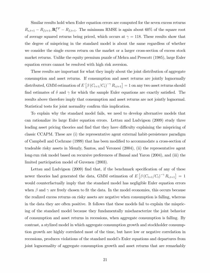
Similar results hold when Euler equation errors are computed for the seven excess returns

+1 − +1R − +1. The minimum RMSE is again about 60% of the square root

of average squared returns being priced, which occurs at = 118 These results show that

the degree of mispricing in the standard model is about the same regardless of whether

we consider the single excess return on the market or a larger cross-section of excess stock

market returns. Unlike the equity premium puzzle of Mehra and Prescott (1985), large Euler

equation errors cannot be resolved with high risk aversion.

These results are important for what they imply about the joint distribution of aggregate

consumption and asset returns. If consumption and asset returns are jointly lognormally

distributed, GMM estimation of £ (+1)

−+1

¤= 1 on any two asset returns should

find estimates of and for which the sample Euler equations are exactly satisfied. The

results above therefore imply that consumption and asset returns are not jointly lognormal.

Statistical tests for joint normality confirm this implication.

To explain why the standard model fails, we need to develop alternative models that

can rationalize its large Euler equation errors. Lettau and Ludvigson (2009) study three

leading asset pricing theories and find that they have difficulty explaining the mispricing of

classic CCAPM. These are (i) the representative agent external habit-persistence paradigm

of Campbell and Cochrane (1999) that has been modified to accommodate a cross-section of

tradeable risky assets in Menzly, Santos, and Veronesi (2004), (ii) the representative agent

long-run risk model based on recursive preferences of Bansal and Yaron (2004), and (iii) the

limited participation model of Guvenen (2003).

Lettau and Ludvigson (2009) find that, if the benchmark specification of any of these

newer theories had generated the data, GMM estimation of £ (+1)

−+1

¤= 1

would counterfactually imply that the standard model has negligible Euler equation errors

when and are freely chosen to fit the data. In the model economies, this occurs because

the realized excess returns on risky assets are negative when consumption is falling, whereas

in the data they are often positive. It follows that these models fail to explain the mispric-

ing of the standard model because they fundamentally mischaracterize the joint behavior

of consumption and asset returns in recessions, when aggregate consumption is falling. By

contrast, a stylized model in which aggregate consumption growth and stockholder consump-

tion growth are highly correlated most of the time, but have low or negative correlation in

recessions, produces violations of the standard model’s Euler equations and departures from

joint lognormality of aggregate consumption growth and asset returns that are remarkably

21

similar to those found in the data. More work is needed to assess the plausibility of this

channel.

In summary, explaining why the standard consumption-based model’s unconditional

Euler equations are violated—for any values of the model’s preference parameters—has so

far been largely elusive, even for today’s leading consumption-based asset pricing theories.

This anomaly is striking because early empirical evidence that the standard model’s Euler

equations were violated provided much of the original impetus for developing the newer mod-

els studied here. Explaining why the standard consumption-based model exhibits such large

unconditional Euler equation errors remains an important challenge for future research, and

for today’s leading asset pricing models.

5 Scaled Consumption-Based Models

A large class of consumption-based models have an approximately linear functional form

for the stochastic discount factor. In empirical work, it is sometimes convenient to use

this linearized formulation rather than estimating the full nonlinear specification. Many

newer consumption-based theories imply that the pricing kernel is approximately a linear

function of current consumption growth, but unlike the standard consumption-based model

the coefficients in the approximately linear function depend on the state of the economy. I

will refer to these as scaled consumption-based models because the pricing kernel is a state-

dependent or “scaled” function of consumption growth and possibly other fundamentals.

Scaled consumption-based models offer a particularly convenient way to represent state-

dependency in the pricing kernel. In this case we can explicitly model the dependence of

parameters in the stochastic discount factor on current period information. This dependence

can be specified by simply interacting, or “scaling,” factors with instruments that summarize

the state of the economy (according to some model). As explained below, precisely the same

fundamental factors (e.g., consumption, housing etc.) that price assets in traditional unscaled

consumption-based models are assumed to price assets in this approach. The difference is

that, in these newer theories of preferences, these factors are expected only to conditionally

price assets, leading to conditional rather than fixed linear factor models. These models can

be expressed as multifactor models by multiplying out the conditioning variables and the

fundamental consumption-growth factor.

As an example of a scaled consumption based model, consider the following approximate

22

formulation for the pricing kernel:

+1 ≈ + ∆+1

Almost any nonlinear consumption-based model can be approximated in this way. For

example, the classic CCAPM with CRRA utility:

() =1−

1− ⇒ +1 ≈ |{z}

=0

− |{z}=0

∆+1 (18)

The pricing kernel in the CCAPM is an approximate linear function of consumption growth

with fixed weights = 0 and = 0. Notice that there is no reason based on this model

of preferences to specify the coefficients in the pricing kernel as functions of conditioning

information; those parameters are constant and known functions of primitive preference pa-

rameters. This does not imply that the conditional moments [+1R+1 − 1] are constant.There may still be a role for conditioning information in the Euler equation, even if there

is no role for conditioning in the linear pricing kernel. This distinction is discussed further

below.

Alternatively, consider the model of Campbell and Cochrane (1999) (discussed further

below), and the closely related model of Menzly, Santos, and Veronesi (2004), with habit

formation and time-varying risk aversion:

( ) =()

1−

1− +1 ≡ −

where is an external habit that is a function of current and past average (aggregate)

consumption and is the so-called “surplus consumption ratio.” In this case the pricing

kernel may be approximated as

+1 ≈ (1− ()− (− 1)) ( − )| {z }=

−(1 + ())| {z }=

∆+1 (19)

where is the log of the surplus consumption ratio, is a parameter of utility curvature,

is the mean rate of consumption growth, is the persistence of the habit stock, and

() is the sensitivity function specified in Campbell and Cochrane. In this model, the

pricing kernel is an approximate state-dependent linear function of consumption growth.

This model provides an explicit motivation for modeling the coefficients in the pricing kernel

23

as functions of conditioning information, something (Cochrane (1996)) refers to as “scaling

factors.” Although the parameters and in (19) are nonlinear functions of the model’s

primitive parameters and state-variable , in equilibrium they fluctuate with variables that

move risk-premia. Proxies for time-varying risk-premia should therefore be good proxies for

time-variation in and if models like (19) are valid.

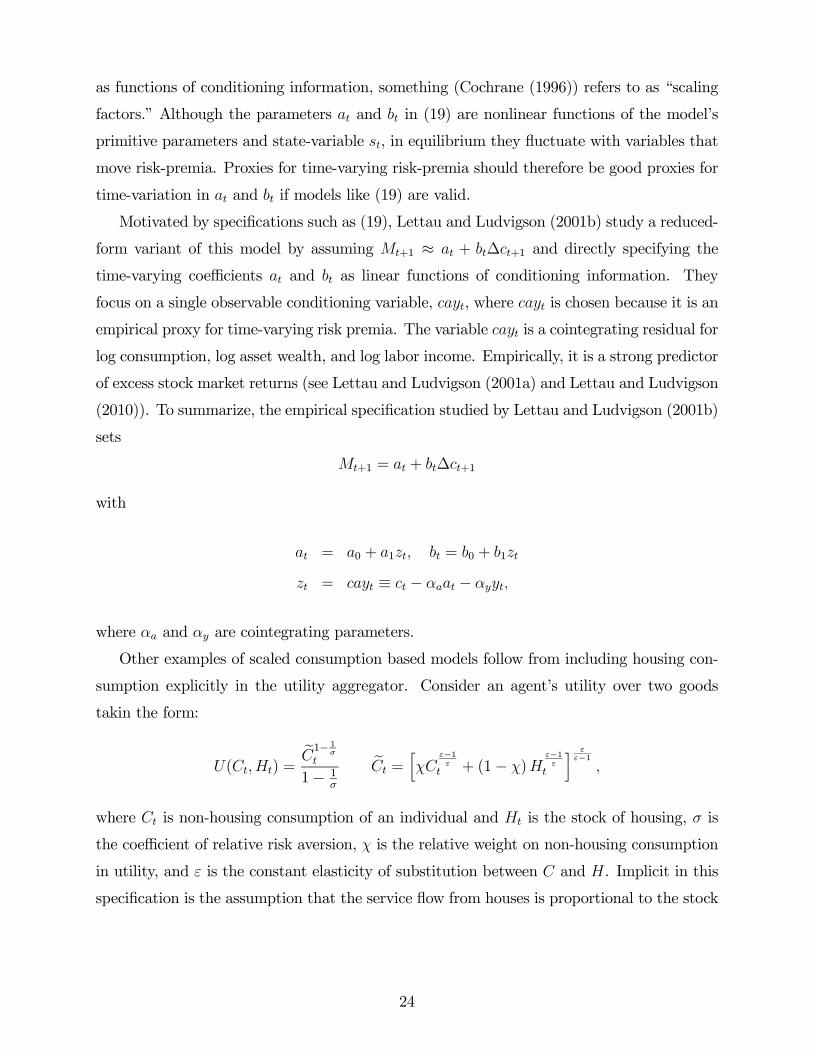
Motivated by specifications such as (19), Lettau and Ludvigson (2001b) study a reduced-

form variant of this model by assuming +1 ≈ + ∆+1 and directly specifying the

time-varying coefficients and as linear functions of conditioning information. They

focus on a single observable conditioning variable, , where is chosen because it is an

empirical proxy for time-varying risk premia. The variable is a cointegrating residual for

log consumption, log asset wealth, and log labor income. Empirically, it is a strong predictor

of excess stock market returns (see Lettau and Ludvigson (2001a) and Lettau and Ludvigson

(2010)). To summarize, the empirical specification studied by Lettau and Ludvigson (2001b)

sets

+1 = + ∆+1

with

= 0 + 1 = 0 + 1

= ≡ − −

where and are cointegrating parameters.

Other examples of scaled consumption based models follow from including housing con-

sumption explicitly in the utility aggregator. Consider an agent’s utility over two goods

takin the form:

( ) =e1− 1

1− 1

e =h

−1

+ (1− )−1

i −1

where is non-housing consumption of an individual and is the stock of housing, is

the coefficient of relative risk aversion, is the relative weight on non-housing consumption

in utility, and is the constant elasticity of substitution between and . Implicit in this

specification is the assumption that the service flow from houses is proportional to the stock

24

. Here the pricing kernel takes the form

+1 =+1

=

⎡⎢⎢⎢⎣µ+1

¶− 1

⎡⎢⎣+ (1− )³+1

+1

´ −1

+ (1− )³

´ −1

⎤⎥⎦−

(−1)⎤⎥⎥⎥⎦ (20)

This model has been studied in its representative agent formulation by Piazzesi, Schnei-

der, and Tuzel (2007). The stochastic discount factor (20) makes explicit the two-factor

structure of the pricing kernel. Piazzesi, Schneider, and Tuzel (2007) show that the log

pricing kernel can be written as a linear two-factor model

ln+1 = + ∆ ln+1 + ∆ ln+1 (21)

where

+1 ≡

+

is the consumption expenditure share on non-housing consumption and and are the

prices of non-housing and housing consumption, respectively. Piazzesi, Schneider, and Tuzel

(2007) focus on the time-series implications of the model. According to the model, the

dividend yield and the nonhousing expenditure share forecast future excess stock returns.

They find empirical support for this prediction and document that the expenditure share at

predicts excess stock returns better than does the dividend yield.

The representation (21) is a multifactor model, but not a scaled multifactor model: the

coefficients on the factors ∆ ln+1 and ∆ ln+1 in the pricing kernel are constant and

known functions of preference parameters. But, because the level of the pricing kernel +1

is nonlinear in the factors +1 and +1, Piazzesi, Schneider, and Tuzel (2007) show

that the log pricing kernel can be approximated as a scaled multifactor model by linearizing

∆ ln+1 around the point +1 = , where +1 ≡ to obtain:

ln+1 ≈ + ∆ ln+1 + (1− ln)∆ ln+1

Lustig and Van Nieuwerburgh (2005) study a model in which households have the same

specification for preferences as in (20) but they dispose of the representative agent formula-

tion, instead studying a heterogeneous agent model with endogenously incomplete markets

(with complete contingent claims but limited commitment) and collateralized borrowing.

25

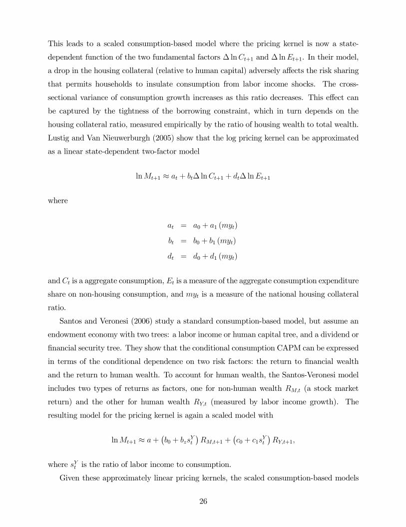
This leads to a scaled consumption-based model where the pricing kernel is now a state-

dependent function of the two fundamental factors ∆ ln+1 and ∆ ln+1. In their model,

a drop in the housing collateral (relative to human capital) adversely affects the risk sharing

that permits households to insulate consumption from labor income shocks. The cross-

sectional variance of consumption growth increases as this ratio decreases. This effect can

be captured by the tightness of the borrowing constraint, which in turn depends on the

housing collateral ratio, measured empirically by the ratio of housing wealth to total wealth.

Lustig and Van Nieuwerburgh (2005) show that the log pricing kernel can be approximated

as a linear state-dependent two-factor model

ln+1 ≈ + ∆ ln+1 + ∆ ln+1

where

= 0 + 1 ()

= 0 + 1 ()

= 0 + 1 ()

and is a aggregate consumption, is a measure of the aggregate consumption expenditure

share on non-housing consumption, and is a measure of the national housing collateral

ratio.

Santos and Veronesi (2006) study a standard consumption-based model, but assume an

endowment economy with two trees: a labor income or human capital tree, and a dividend or

financial security tree. They show that the conditional consumption CAPM can be expressed

in terms of the conditional dependence on two risk factors: the return to financial wealth

and the return to human wealth. To account for human wealth, the Santos-Veronesi model

includes two types of returns as factors, one for non-human wealth (a stock market

return) and the other for human wealth (measured by labor income growth). The

resulting model for the pricing kernel is again a scaled model with

ln+1 ≈ +¡0 +

¢+1 +

¡0 + 1

¢+1

where is the ratio of labor income to consumption.

Given these approximately linear pricing kernels, the scaled consumption-based models

26

above are all tested on unconditional Euler equation moments: [+1R+1] = 1. The

papers above then ask whether the unconditional covariance between the pricing kernel and

returns can explain the large spread in unconditional mean returns on portfolios of stocks

that vary the basis of size (market capitalization) and book-to-market equity ratio.

5.1 Econometric Findings

The studies above find that state-dependency in the linear pricing kernel greatly improves

upon the performance of the unscaled counterpart with constant coefficients as an explana-

tion for the cross-section of average stock market returns. Explaining the cross-section of

returns on portfolios sorted according to both size and book-to-market equity has presented

one of the greatest challenge for theoretically-based asset pricing models such as the static

CAPM of Sharpe (1964) and Lintner (1965), and the classic CCAPM discussed above. The

strong variation in returns across portfolios that differ according to book-to-market equity

ratios cannot be attributed to variation in the riskiness of those portfolios, as measured by

either the CAPM (Fama and French (1992)) or the CCAPM (see discussion below). Fama

and French (1993) find that financial returns related to firm size and book-to-market equity,

along with an overall stock market return, do a good job of explaining the cross-section of

returns on these portfolios. If the Fama—French factors truly are mimicking portfolios for un-

derlying sources of macroeconomic risk, there should be some set of macroeconomic factors

that performs well in explaining the cross-section of average returns on those portfolios.

Lettau and Ludvigson (2001b) find that the scaled consumption CAPM, using aggregate

consumption data, can explain about 70 percent of the cross-sectional variation in average

returns on 25 portfolios provided by Fama and French, which are portfolios of individuals

stocks sorted into five size quantiles and five book-market quantiles (often referred to as the

25 Fama-French portfolios). This result contrasts sharply with the 1 percent explained by the

CAPMand the 16% explained by the standard (unscaled) CCAPMwhere = (1− ∆).

The consumption factors scaled by are strongly statistically significant. An important

aspect of these results is that the conditional consumption model, scaled by , goes a

long way toward explaining the celebrated “value premium,” that is the well documented

pattern found in average returns that firms with high book-to-market equity ratios have

higher average returns than do firms with low book-to-market ratios.

Similar findings are reported for the other scaled consumption based models. Lustig

and Van Nieuwerburgh (2005) find that, conditional on the housing collateral ratio, the

27

covariance of returns with aggregate risk factors ∆ ln+1 and ∆ ln+1 explains 80 percent

of the cross-sectional variation in annual size and book-to-market portfolio returns. Santos

and Veronesi (2006) find empirically that conditioning market returns on dramatically

improves the cross-sectional fit of the asset pricing model when confronted with size and

book-market portfolios of stock returns.

These scaled consumption-based models of risk are conceptually quite different models of

risk from their unscaled counterparts. Because the pricing kernel is a state-dependent func-

tion of consumption growth, assets are risky in these models not because they are more highly

unconditionally correlated with consumption growth (and other fundamental factors), but

because they are more highly correlated with consumption in bad times, when the economy

is doing poorly and risk premia are already high. Lettau and Ludvigson (2001b) provide

direct evidence of this mechanism, by showing that returns of value portfolios are more

highly correlated with consumption growth than are growth portfolios in downturns, when

risk/risk aversion is high (whend is high), than in booms, when risk/risk aversion is low(d is low). Because these results are based on estimates of unconditional Euler equationrestrictions, they follow only from state-dependency in the pricing kernel and are illustrated

using empirical restrictions that do not incorporate or depend on conditioning information

in the Euler equation. This is discussed further below.

5.2 Distinguishing Two Types of Conditioning

With reference to scaled consumption-based models, it is important to distinguish two types

of conditioning. One type occurs when we seek to incorporate conditioning information into

the moments [+1+1] = 1 written

[+1+1|x] = 1

where x is the information set of investors upon which the joint distribution of +1+1

is based. This form of conditionality, to which Cochrane (1996) refers as “scaling returns,”

captures conditioning information in the Euler equation:

[+1(+1 ⊗ (1 x)0)] = 1 (22)

28

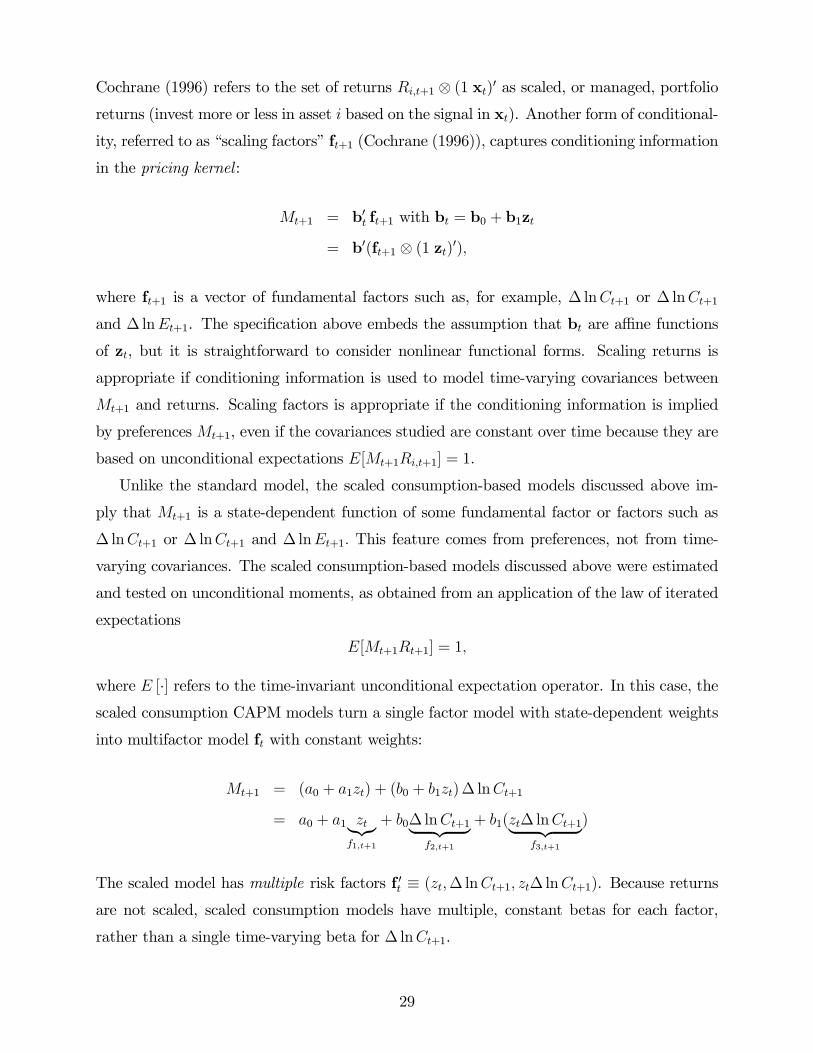
Cochrane (1996) refers to the set of returns +1 ⊗ (1 x)0 as scaled, or managed, portfolioreturns (invest more or less in asset based on the signal in x). Another form of conditional-

ity, referred to as “scaling factors” f+1 (Cochrane (1996)), captures conditioning information

in the pricing kernel :

+1 = b0 f+1 with b = b0 + b1z

= b0(f+1 ⊗ (1 z)0)

where f+1 is a vector of fundamental factors such as, for example, ∆ ln+1 or ∆ ln+1

and ∆ ln+1. The specification above embeds the assumption that b are affine functions

of z, but it is straightforward to consider nonlinear functional forms. Scaling returns is

appropriate if conditioning information is used to model time-varying covariances between

+1 and returns. Scaling factors is appropriate if the conditioning information is implied

by preferences+1, even if the covariances studied are constant over time because they are

based on unconditional expectations [+1+1] = 1.

Unlike the standard model, the scaled consumption-based models discussed above im-

ply that +1 is a state-dependent function of some fundamental factor or factors such as

∆ ln+1 or ∆ ln+1 and ∆ ln+1 This feature comes from preferences, not from time-

varying covariances. The scaled consumption-based models discussed above were estimated

and tested on unconditional moments, as obtained from an application of the law of iterated

expectations

[+1+1] = 1

where [·] refers to the time-invariant unconditional expectation operator. In this case, thescaled consumption CAPM models turn a single factor model with state-dependent weights

into multifactor model f with constant weights:

+1 = (0 + 1) + (0 + 1)∆ ln+1

= 0 + 1 |{z}1+1

+ 0∆ ln+1| {z }2+1

+ 1(∆ ln+1| {z }3+1

)

The scaled model has multiple risk factors f 0 ≡ (∆ ln+1 ∆ ln+1). Because returns

are not scaled, scaled consumption models have multiple, constant betas for each factor,

rather than a single time-varying beta for ∆ ln+1.

29

To see this, we derive the beta-representation for this model. A beta representation

exists only for formulations of the pricing kernel in which it is an affine function of factors.

Let F = (1 f 0)0, denote the vector of these multiple factors including a constant and let

= b0F, and ignore time indices. From the unconditional Euler equation moments we have

1 = []⇒ unconditional moments (23)

= [F0]b

= [][F0]b+Cov(F

0)b

Let b denote the coefficients on variable factors f 0. Then

[] =1−Cov(F

0)b[F0]b

=1−Cov( f

0)b[F0]b

=1−Cov( f

0)Cov(f f 0)−1Cov(f f 0)b[F0]b

= −0β0Cov(f f0)b

= − β0λβ0λ ⇒ multiple, constant betas β (24)

where

β0 ≡ Cov( f0)Cov(f f 0)−1

λ ≡ Cov(f f 0)b

This gives rise to an unconditional multifactor, scaled consumption-based model with mul-

tiple β’s, e.g.,:

+1 = + ∆∆+1 + ∆∆+1 + + +1 = 1 (25)

30

where +1 is an expectational error for +1. The above equation can be re-written as

+1 = + (∆ + ∆)| {z }

∆+1 + + +1 = 1

where is a time-varying consumption beta that applies specifically to the unconditional,

scaled multifactor model = b0F and 1 = [] for any traded asset indexed by . I will

refer to as the scaled consumption beta.

It is important to emphasize that the time-varying beta is not the same as the

conditional consumption beta of the classic consumption-CAPM (8). Instead, arises from

an entirely different model of preferences in which the pricing kernel is a state-dependent

function of consumption growth. In the standard model there are no scaled factors because

the coefficients in the linear pricing kernel (18) are constant and known functions of preference

parameters. Nevertheless, a conditional consumption beta may be derived for the standard

model from time-variation in the conditional moment (+1R+1) = 1, where +1 =

[+1]−. Using the linearized form of this model = (1− ∆), conditionality in

the Euler equation (+1R+1) = 1 gives rise to a time-varying beta

=Cov (∆ )

Var (∆)

Movements in the conditional consumption beta reflect the role of conditioning infor-

mation in the Euler equation of the standard consumption-based model. could vary, for

example, if the covariance between consumption growth and returns varies over time. By

contrast, movements in the reflect state-dependency of consumption growth in the pricing

kernel itself, driven, for example, by time-varying risk aversion, or the tightness of borrow-

ing constraints in an incomplete markets setting. Thus and represent two different

models of consumption risk. The former is based on an approximately linear pricing kernel

that is a state-dependent function of consumption growth, whereas the latter is based on

an approximately linear pricing kernel that is a state-independent function of consumption

growth.

The statistic is also not the same as the conditional consumption beta of a scaled

consumption-based model, +1 = b0F+1 because it is estimated from unconditional Euler

equation moments. In particular, its estimation does not for example use any scaled returns.

A conditional consumption beta may be estimated for models with scaled factors, but this

31

requires explicitly modeling the conditioning information in the Euler equation, or the joint

conditional distribution of +1 and test asset returns:

1 = [+1+1]

= [b0F+1+1]⇒

[+1] = +1 − 0 (26)

where 0 now represents the conditional consumption beta of the scaled model.

Whether it is necessary or desirable to include conditioning information in the Euler

equation depends on the empirical application. A necessary condition for estimating and

testing models of using GMM is that the number of Euler equation moments be at least

as large as the number of parameters to be estimated. This implies that the econometrician’s

information set need not be the same as investors. Indeed, if we have enough test asset returns

the model can be estimated and tested by “conditioning down” all the way to unconditional

moments, as in the studies discussed above. This is possible because GMM theory is based

on the unconditional moments {h (θw+1)} = 0. Conditioning information can always

be incorporated by including instruments x observable at time , as in (16), but those are

already imbedded in h (θw+1). Importantly, for the purpose of estimating and testing the

model, there is no need to identify the true conditional mean [+1+1 − 1] based on theinformation set of investors. (The relevance of this is discussed further below in Section 6.2 in

the context of estimating semiparametric models where, by contrast, the identification of the

conditional mean is required.) But note that this is an asymptotic result: in finite samples,

the estimation and testing of economic models by GMM can, and often does, depend on the

information set chosen. More generally in finite samples the results of GMM estimation can

depend on the choice of moments that form the basis for econometric evaluation.

It is important to distinguish the task of estimating and testing a particular model for

+1 using GMM, (which can be accomplished asymptotically on any set of theoretically

appropriate unconditional moments as long they are sufficient to identify the primitive pa-

rameters of interest), from other tasks in which we may need an estimate of the conditional

moments themselves, such as for example when we want to form inferences about the behav-

ior of the conditional consumption beta . In the latter case, we need to identify the true

conditional moment, which depends on the information set of economic agents. This poses

a potential problem. As Cochrane (2005) emphasizes, the conditioning information of eco-

32

nomic agents may not be observable, and one cannot omit it in making inferences about the

behavior of conditional moments. Hansen and Richard (1987) show that the mean-variance

implications of asset pricing models are sensitive to the omission of conditioning information.

The identification of the conditional mean in the Euler equation requires knowing the joint

distribution of +1 and the set of test asset returns Rt+1. An econometrician may seek to

approximate this conditional joint distribution, but approximating it well typically requires

a large number of instruments that grow with the sample size, and the results can be sensi-

tive to chosen conditioning variables (Harvey (2001)). In practice, researchers are forced in

finite samples to choose among a few conditioning variables because conventional statistical

analyses are quickly overwhelmed by degrees-of-freedom problems as the number rises. If

investors have information not reflected in the chosen conditioning variables, measures of

conditional mean will be misspecified and possibly misleading.3

For this reason is often convenient to focus on empirical restrictions that do not depend

on conditioning information in the Euler equation, as in the tests carried out in the scaled

consumption-based literature that are based on the models’ unconditional Euler equation

implications. Hansen and Richard (1987) show that conditioning down per se does not

prevent the researcher from distinguishing between different models of the pricing kernel.

What is required is a model of the pricing kernel+1. This in turn requires the researcher to

take a stand on the scaling variables in the pricing kernel. In the case of scaled consumption-

based models, theory may provide guidance as to the choice of scaling variables that are

part of the SDF (e.g., housing collateral ratio, or labor share), typically a few observable

instruments that summarize time-varying risk-premia.

Of course, scaling factors is one way to incorporate conditioning information–into the

pricing kernel. Some authors (e.g., Lettau and Ludvigson (2001b)) therefore used the terms

“scaling” and “conditioning” interchangeably when referring to models with scaled factors

even though the models were estimated and tested on unconditional Euler equation moments.

An unfortunate consequence of this “conditional” terminology may have been to create

the mis-impression (discussed below) that scaled consumption-based factor models provided

estimates of the conditional CCAPM beta even though, unlike , the conditional beta

is always derived from conditional Euler equation moments (scaling returns), whether or not

the pricing kernel includes scaled factors. Mea culpa.4

3A partial solution is to summarize information in large number of time-series with few estimated dynamic

factors (e.g., Ludvigson and Ng 2007, 2009).4On page 1248 of their published paper, Lettau and Ludvigson (2001b) distinguish the two forms of

33

5.3 Debate

Lewellen, Nagel, and Shanken (2010) (LNS) take a skeptical view of the asset pricing tests

of a number of macroeconomic factor models found in several papers, including the scaled

consumption-based models discussed above. Their paper offers a number of specific sug-

gestions, designed to “raise the bar” in the statistical evaluation of asset pricing models.

Several suggestions are sensible checks on the finite sample properties of test statistics, such

as the recommendation to report confidence intervals for test statistics rather than relying

merely on point estimates. Other recommendations include testing models on assets other

than the size and book-market sorted portfolios commonly used, reporting GLS R-squared

statistics, and imposing a more complete set of theoretical restrictions on parameter esti-

mates along the lines suggested by Lewellen and Nagel (2006) (discussed below). Once all

of these recommendations have been implemented, the authors find that none of the many

proposed macroeconomic models of the SDF performs well in explaining a cross-section of

average stock returns.

LNS also find, however, that the same disappointing results apply to the Fama-French

three-factor model, which explains over 90% of the time-variation in size and book-market

portfolio returns and is implicitly treated as the true model in their analysis. Indeed, the

results in Table 1 of LNS show that the Fama-French model performs no better than the other

consumption-based models when confronted with industry returns and evaluated according

to the GLS R-squared statistic. These findings suggest that none of the evaluated models

are free of specification error, including even very well fitting empirical specifications such as

the Fama-French three-factor model. But the findings also provide no way of distinguishing

among models that are all misspecified: an informal ranking of models is hardly changed

by these additional diagnostics. In particular, the findings are not evidence against the

conclusion that incorporating state dependency into the pricing kernel improves the fit of

unscaled factor models.

These issues are all statistical in nature; they pertain to whether a given model is correctly

specified or not. Yet, despite the several statistical checks they recommend, Lewellen, Nagel,

and Shanken (2010) argue that their primary point has nothing to do with statistical error.

Instead, they argue, because the Fama-French three factors explain more than 90% of the

conditionality and emphasize that, because their estimates are based on unconditional Euler equations, they

do not deliver an estimate of the conditional covariance of factors with returns, as required to form inferences

about the conditional consumption beta for the scaled model, or the conditional price of consumption risk

.

34

time-variation in realized returns on the size and book-market sorted portfolios that are

typically used to evaluate the consumption-based models, any three-factor model with factors

that are correlated with the Fama-French factors (and not with the small idiosyncratic

component of returns that is unrelated to these factors), will explain the data as well as the

Fama-French model according to any statistical metric. This suggestion implies that any

proposed three-factor model with factors weakly correlated with the Fama-French factors

could be observationaly equivalent to the Fama-French model or to any “true” model. But

since they are all observationaly equivalent in this case, the answer to this debate cannot be

settled statistically, but must instead lie with economic theory.

Economic theory implies that the true sources of systematic risk must be macroeconomic

in nature. The Fama-French factors or other return-based factors may be mimicking port-

folios for the true underlying sources of risk, but we can’t hope to explain returns in terms

of economic shocks with models of other returns. Economics therefore drives us back to the

importance of evaluating macroeconomic models of risk. To the extent that multiple models

are observationaly equivalent statistically, we are left with only macroeconomic theory as

our guide. Moreover, the observations of Lewellen, Nagel, and Shanken (2010) leave open

the question of why those macroeconomic models that do help explain returns are correlated

with the Fama-French factors. One possibility is that the Fama-French factors are mimicking

portfolios for the true sources of macroeconomic risk. In practice, however, models often can

be distinguished statistically and we know that many macroeconomic models do not explain

the size and book-market returns. Empirical findings such as those in LNS underscore the

need for econometric tests that permit the statistical comparison of multiple competing mod-

els, allowing all models to be misspecified. I discussed one such approach to this problem

above, for statistically comparing HJ distances across multiple models.

What of findings in the literature that suggest a number of macroeconomic factor models

may help explain the size and book-market effects in portfolio returns? LNS raise this as a

cause for suspicion, arguing that it offers an embarrassment of riches. But macroeconomic

risk is by nature characterized by common variation among large number of economic time

series, as occurs in business cycles for example. Moreover, only weak theoretical restrictions

are required to obtain a factor structure in large data-sets (Chamberlain and Rothschild

(1983)). Therefore, if economic theory is correct and systematic risk is macroeconomic in

nature, we should expect a factor structure in macroeconomic data, and we should expect a

35

variety of macroeconomic indicators to be correlated with these factors.5 These considera-

tions suggest that we should be neither surprised nor alarmed by the observation that several

macroeconomic models of risk help explain financial market behavior. But perhaps what’s

really at stake here is the idea that there is a single, true model that explains all aspects

of the data to the exclusion of all others. All of the models considered by LNS may have

elements of the truth, and the question is whether we learn anything from knowing that a

specification that is misspecified may still help us interpret important aspects of the data.

Lewellen and Nagel (2006) (LN) present a more specific criticism of the conditional CAPM

based on a novel test that estimates time-varying CAPM betas using high-frequency data

on asset returns and short window regressions. They argue that conditional CAPM betas so

estimated are not volatile enough to explain the large excess returns on size and book-market

sorted portfolios.

These empirical tests cannot be directly applied to the consumption CAPM, because of

the absence of high frequency consumption data. Nevertheless, Lewellen and Nagel (2006)

still argue informally, taking as an example the findings of Lettau and Ludvigson (2001b)

(LL), that estimates of the scaled consumption-based models are unlikely to explain the data

and may violate restrictions implied by the conditional CCAPM.

The argument can be explained as follows. LN begin with a statement of the conditional

CCAPM as6

£+1

¤= (27)

≡cov (∆ )

var (∆)

where +1 is the stock’s excess return, is the conditional CCAPM beta and is the

time price of consumption beta risk. Note that in (27) is the conditional beta from

the classic consumption-CAPM (8) model of risk. Take unconditional expectations of (27)

to obtain

£+1

¤=

£¤ [] + cov

¡

¢ (28)

As in (25), the three factor scaled consumption-based model estimated by LL with factors

5Ludvigson and Ng (2007, 2009) find evidence of a factor structure in large datasets of macroeconomic

variables that are related to bond and stock returns.6The timing notation used here differs from that of LN who denote conditional moments for period

given − 1 information with a subscript rather than with a − 1 subscript, as here.

36

f = [∆∆−1 −1]0and −1 = −1 relates returns to factors over time:

+1 = + ∆∆+1 + ∆∆+1 + + +1 = 1 (29)

where the unconditional beta vector β =£∆ ∆

¤0is obtained from a multiple

regression of returns on factors f:

β0 = cov (f f0)−1cov (f )

(Note that an unconditional beta is not the mean of the conditional beta, so 6= £¤)

As above, (29) may be trivially re-written as

+1 = + (∆ + ∆)| {z }

∆+1 + + +1 = 1 (30)

If we take unconditional expectations on both sides of (29), we obtain a relation between

average returns and betas, where the betas are multiplied by constant coefficients (·):

[+1] = + ∆∆ + ∆∆ + = 1 (31)

The constant and coefficients (·) may be consistently estimated using a second-stage Fama-

MacBeth regression (Fama and MacBeth (1973)) of average returns on multiple betas.7

With these features of the LL model in hand, LN seek to derive restrictions on the

parameters of the scaled consumption-based model by using as an estimate for and

substituting it into the covariance term in (28), thus obtaining

£+1

¤=

£¤ [] + cov

¡

¢(32)

or

£+1

¤=

£¤ [] + ∆cov ( ) (33)

With this substitution, LN equate (33) and (31). Comparing (33) and (31), LN argue that,

7The asset pricing model implies that must be either zero (in the case of excess returns) or equal tothe zero-beta rate (in the case of raw returns). This in turn places restrictions on the time-series intercepts

in (30), as discussed further below.

37

with

∆ = []

∆∆ = £¤ [] (34)

and

∆∆ = ∆cov ( ) (35)

it may be concluded that

∆ = cov ( ) ≤ (36)

where (·) denotes the standard deviation of the generic argument (·). According to thisreasoning, ∆ is an estimate of cov( ), which must obey the inequality on the right-

hand-side of (36) since correlations are less than one in absolute value. LL provide estimates

of ∆ and with = With these estimates, LN argue that the inequality in (36)

places restrictions on the magnitude of . In particular, given the estimates of ∆ around

0.06% or 0.07% per quarter, and given the estimate of , they argue that must be large

(greater than 3.2% quarterly) in order to satisfy the inequality in (36). At the same time

LN note that the reported value of ∆, which they take to be an estimate of [], is small.

LN claim that the combination of large and small [] is inconsistent, quantitatively,

with some consumption-based models.

The reasoning behind the calculations above can be challenged on several levels, all of

which pertain to the equating of (33) and (31) from which (34) and (35) follow and from

which the inequality restriction (36) is derived. First, ∆ 6= £¤, as required by (34).

The parameter ∆ is not an estimate of the unconditional consumption beta for the standard

model. Even if it were, it would not in general be equal to the mean of the conditional beta.

Second, (31) contains the additional term , absent in (33). As a result, if ∆ and

are correlated, as is likely, ∆ will be a biased estimate of cov( ) Third, as noted

above, is not an estimate of the conditional consumption beta and therefore the

substitution of for into the covariance term of equation (32) is questionable. The

fundamental difficulty in each of these steps is that the parameters from the LL estimation

come from a procedure that delivers multiple, constant betas as in (24), rather than a single,

time-varying beta as required by the LN calculation. In summary, even if it were true that

some consumption-based models are inconsistent with a value for that is both highly

volatile and low on average, the estimates in LL are not informative on this matter and

38

calculations of the type outlined above cannot be taken as evidence against the approximate

models of risk studied there.

What is the time-varying beta if not a conditional CCAPM beta? The implied

parameter is a statistic useful for illustrating intuitively why conditioning in the pricing

kernel explains return data better than its unscaled counterpart even when the model is

estimated and tested on unconditional Euler equation moments. It is a summary statistic

that helps explain why the presence of, e.g., time-varying risk aversion, or time-varying

risk-sharing, changes the concept of risk, from one involving a state-independent function

of consumption growth to one involving a state-dependent function. Put differently, the

statistic is a convenient way of summarizing why both ∆+1 and ∆+1 matter for

risk. But the derivation of follows only from state-dependency in the pricing kernel and

is illustrated using empirical restrictions that do not incorporate or depend on conditioning

information in the Euler equation. For this reason, is not an estimate of and it

is therefore not useful for illustrating the dynamics of the conditional joint distribution

of consumption and returns in the standard consumption CAPM. It is also not useful for

illustrating the dynamics of the conditional joint distribution of consumption and returns in

the newer scaled consumption-based models because, here also, the conditional consumption

beta must be inferred from an estimation of the conditional time- Euler equation (26),

rather than from the unconditional Euler equation (23). This could be accomplished, for

example, by estimating the scaled factor model on (a sufficiently large set of) scaled returns,

or managed portfolio returns.8

Of course, none of these observations imply that the scaled consumption based model

is perfectly specified. Indeed, even the original papers that studied these models suggested

that some theoretical restrictions were not satisfied. For example, the implied zero-beta rate

in the estimates of Lettau and Ludvigson (2001b) are implausibly large.

A separate criticism of the empirical tests of scaled consumption-based models points to

the failure of these tests to impose a different type of restriction, one involving the time-series

intercepts in the first-pass time-series regression used to estimate betas. In the introduction

of their paper, LN suggest that one reason the conclusions of LL, Jagannathan and Wang

(1996), Lustig and Van Nieuwerburgh (2005), and Santos and Veronesi (2006) differ from

8Alternatively, conditional consumption betas could be inferred from a flexible estimation of the condi-

tional joint distribution of the pricing kernel and all test asset returns using semi-nonparametric techniques,

as in (Gallant and Tauchen (1989)), or from a variety of other approaches to estimating conditional Euler

equation moments, as in Duffee (2005), Nagel and Singleton (2010) or Roussanov (2010). These papers are

discussed further below.

39

their own is that these studies focus on cross-sectional regressions and not on time-series

intercept tests. Indeed, the published versions of these studies all evaluate the performance

of their models solely on the basis of cross-sectional regressions. This approach requires an

estimate of the time-series intercept in first-pass regressions such as (29). But the time-

series intercepts in each of these studies are estimated freely, without imposing restrictions

implied by the theory. Specifically, the restrictions

= β0(1)

(λ−(f))| {z }(1)

, = 1 2 (37)

where is the number of multiple factors in f of each model, are not imposed. To derive

this restriction, note that, with excess returns, , the multiple betas of each model are

estimated from a first pass time-series regression taking the form

= + β

0f + = 1 2 (38)

The asset pricing model is:

() = β0λ = 1 2 (39)

Taking expectations of (38),

() = + β

0E(f ), = 1 2 (40)

and equating (39) and (40), we obtain the restriction (37). Notice that the time-series

intercept restrictions (37) are distinct from the presumed inequality restriction (36) upon

which Lewellen and Nagel (2006) focus.

Although ignored in the published studies, the time-series intercept restrictions may be

imposed and tested as follows. Consider the time-series regression of excess returns on

factors:

= + β

0f + ; = 1 2

Stacking the data on asset returns and factors into vectors, the moments for the

40

unrestricted OLS time-series regression are

( R

(1)

− a(×1)

− β0()

f(1)

) = 0

"(R

(1)

− a(×1)

− β0()

f(1)

)⊗ f(1)

#= 0

where “” denotes the sample mean in a sample of size . Imposing the restriction (37),

the system becomes:

(R − β0(λ− E(f ))− β0f ) = 0 (41)

[{R − β0(λ− E(f ))− β0f }⊗ f] = 0 (42)

Equations (41) and (42) can be estimated as a system using GMM along with a set of

moment conditions for estimating the means μ of factors:

[f −μ] = 0 (43)

As a result of imposing the restrictions (37) the system (41)-(43) is overidentified: there are

a total of + · + equations and · + 2 parameters to be estimated in β, λ

and μ, or − overidentifying restrictions. These restrictions can be tested using the test

statistic of Hansen (1982):

≡ g(θ;y )0S−1g(θ;y ) ∼ 2( −) (44)

where the sample moments g(θ;y ) (see notation in Section 3) are defined for the three

equations (41)-(43) stacked into one system. The overidentifying restrictions are a test

of whether the model is correctly specified when the time-series intercept restrictions are

imposed.

The table below reports the test statistic for this test and associated -value for the

moment conditions corresponding to the scaled consumption-based model (29), using the

original data employed by Lettau and Ludvigson (2001b) for cross-sections of 6 and 10 size

and book-market portfolio returns.

41

Table 1

Model (6 assets) (10 assets)

(-value) (-value)

Scaled CCAPM 0.02595 0.08662

(0.99889) (0.99999)

Fama-French 0.04875 0.06348

(0.99718) (0.99999)

Table 1 shows that there is no evidence against the restrictions, either for the scaled

CCAPM or the Fama-French three-factor model. The probability of obtaining a statistic

at least as large as that obtained, assuming that the model is true, is very high. The results

therefore provide no evidence that the success of the scaled models (or the Fama-French

three factor model) is attributable to the failure to impose restrictions on the time-series

intercepts.

There are other ways to evaluate whether the time-series intercept restrictions are satisfied

in scaled consumption-based models. For models of the SDF in which factors are returns, the

estimated intercepts from time-series regressions of test asset returns on the factors should

be jointly zero if the model is correctly specified. Kim (2010) forms maximum correlation

portfolios (MCPs) for each of the multiple factors in the scaled CCAPM models investigated

in Lettau and Ludvigson (2001b), and Lustig and Van Nieuwerburgh (2005). By employing

MCP returns that are maximally correlated with the original factors, tests of the models

collapse to evaluating the implication that the time-series intercepts must be jointly zero.

Based on this analysis and the use of size and book-market sorted portfolio returns, Kim

finds that the multifactor scaled CCAPM models have lower average squared pricing errors

than their unscaled counterparts, but that a GRS test (Gibbons, Ross, and Shanken (1989))

almost always rejects the null that the time-series intercepts for each model are jointly zero

for almost all models evaluated, including the Fama-French three factor model. The one

exception is the scaled housing collateral model of Lustig and Van Nieuwerburgh (2005).

Duffee (2005), Nagel and Singleton (2010) and Roussanov (2010) take another approach

to evaluating scaled consumption-based models: they ask whether the conditional implica-

tions of these models are satisfied in the data. In particular, these papers seek to test the

restrictions implied by (7) or (22) for each model, which is a function of conditional moments.

Their objective is to test the conditional, rather than unconditional, Euler equation restric-

42

tions by evaluating the model on scaled returns. Duffee (2005) forms statistical measures

of the conditional covariance between aggregate stock returns and aggregate consumption

growth. He finds, using a few chosen conditioning variables, that this covariance varies over

time. He also finds, however, that the estimated conditional covariance is negatively rather

than positively correlated with his estimate of the conditional expected excess stock market

return, a finding that is inconsistent with consumption-based asset pricing models. Nagel and

Singleton (2010) and Roussanov (2010) also test the conditional implications of scaled models

and make similar points, the former using basis functions of a few conditioning variables to

capture conditional moments that are chosen with the aim of minimizing the variance of the

GMM estimator, the latter using a nonparametric kernel regression to estimate covariances

and a novel approach to estimating risk-prices.9 These researchers conclude that, once the

conditional implications of models with approximately linear but state-dependent pricing

kernels are investigated, the models do not perform well in explaining cross-sectional return

data. These findings suggest that scaled consumption-based models may have more success

satisfying the unconditional Euler equations implied by asset pricing theory than they do

conditional Euler equation restrictions.

As discussed above, the conclusions about the behavior of conditional moments in finite

samples may rely critically on the chosen instruments used to model the conditional mo-

ments. In principle, the conditional joint distribution of the pricing kernel and asset returns

depends on every variable in investors’ information sets and every measurable transforma-

tion thereof, a potentially very large number. It may therefore be difficult if not impossible

to approximate conditional moments well in finite samples, and in practice the results de-

pend on the conditioning information chosen. As Cochrane (2005) emphasizes, investors’

information sets are unobservable, and “the best we can hope to do is to test implications

conditioned down on variables that we can observe and include in a test.”10 As such, find-

ings like those of Duffee (2005), Nagel and Singleton (2010) and Roussanov (2010) certainly

provide no evidence in favor of the consumption-based models, but we cannot conclude that

they provide definitive evidence against the models.

9Like Nagel and Singleton (2010), Lettau and Ludvigson (2001b) also studied the performance of the

-scaled CCAPM in explaining a set of managed portfolio returns, where the original size and book-

market sorted test asset returns were scaled by conditioning information in . In contrast to Nagel andSingleton, Lettau and Ludvigson found that the scaled, multifactor CCAPM performed well, better than the

Fama-French three factor model, in explaining these scaled returns. A number of factors may explain the

discrepancy in results, including different samples and the different methodology Nagel and Singleton apply

to select conditioning instruments optimally from a statistical standpoint.10Chapter 8, Section 8.3.

43

A final point is worth noting regarding tests of the conditional implications of an asset

pricing model. Tests of the conditional asset pricing moments are tests of whether the

model can explain “managed portfolios,” portfolios formed by taking the original test assets

and scaling the returns of those assets by conditioning variables known at time . Tests

of the conditional Euler equation restrictions are therefore tests of whether the model can

explain a set of asset returns that may be quite different from the original (unscaled) test

asset returns. As such, the same points made in Section 3 apply here. By incorporating

conditioning information into the Euler equation, the resulting GMM objective becomes

a test of the model on a re-weighted portfolio of the original test assets. If the original

test assets were carefully chosen to represent interesting economic characteristics, and/or if

the scaled returns do not produce a large spread in average returns, and/or if the scaled

returns imply implausible long and short positions in test assets, tests of the conditional

implications of the model may be less compelling than tests of the unconditional implications

[+1R+1] = 1.

In summary, the body of evidence in these papers suggests that scaled consumption-based

models are unlikely to be perfectly specified. This does not answer the question of whether

the scaled models explain the data better than their unscaled counterparts, or indeed better

than any relevant benchmark. That is because all of the tests discussed in this section are

tests of correct specification against the alternative of incorrect specification. I have argued

above that what we learn from such tests is limited once we acknowledge that all models are

to some degree misspecified. This leaves us with a need for statistical procedures that permit

comparison of model misspecification across multiple competing frameworks. And while it

is tempting to conclude that such a comparison can be made on the basis of whether or not

tests of the null of correct specification (e.g., tests) are rejected for different models, as

Section 3 explains, this practice is not valid because the distribution of the test statistic in

these cases depends on a model-specific estimator that rewards stochastic discount factor

volatility and is not comparable across models.

6 Asset Pricing With Recursive Preferences

As consumption-based asset pricing has progressed, there has been a growing interest in

asset pricing models formed from recursive preferences, especially those of the type studied

by Epstein and Zin (1989), Epstein and Zin (1991), andWeil (1989). I will use EZW as short-

44

hand for this specific form of recursive preferences, defined precisely below. There are at least

two reasons recursive utility is of growing interest. First, the preferences afford a far greater

degree of flexibility as regards attitudes toward risk and intertemporal substitution than does

the standard time-separable power utility model. Second, asset pricing models formed from

such preferences contain an added risk factor for explaining asset returns, above and beyond

the single consumption risk factor found in the standard consumption-based model.

Despite the growing interest in recursive utility models, econometric work aimed at es-

timating the relevant preference parameters and assessing the model’s fit with the data has

proceeded slowly. The EZW recursive utility function is a constant elasticity of substitution

(CES) aggregator over current consumption and the expected discounted utility of future

consumption. This structure makes estimation of the general model challenging because the

intertemporal marginal rate of substitution is a function of the unobservable continuation

value of the future consumption plan. One approach to this difficulty, based on the insight

of Epstein and Zin (1989), is to exploit the relation between the continuation value and the

return on the aggregate wealth portfolio. To the extent that the return on the aggregate

wealth portfolio can be measured or proxied, the unobservable continuation value can be

substituted out of the marginal rate of substitution and estimation can proceed using only

observable variables (e.g., Epstein and Zin (1991), Campbell (1996), Vissing-Jorgensen and

Attanasio (2003)).11 Unfortunately, the aggregate wealth portfolio represents a claim to

future consumption and is itself unobservable. Moreover, given the potential importance of

human capital and other unobservable assets in aggregate wealth, its return may not be well

proxied by observable asset market returns.

These difficulties can be overcome in specific cases of the EZW recursive utility model.

For example, if the EIS is restricted to unity and consumption follows a loglinear vector time-

series process, the continuation value has an analytical solution and is a function of observable

consumption data ( e.g., Hansen, Heaton, and Li (2008)). Alternatively, if consumption and

asset returns are assumed to be jointly lognormally distributed and homoskedastic (e.g., At-

tanasio and Weber (1989)), or if a second-order linearization is applied to the Euler equation,

the risk premium of any asset can be expressed as a function of covariances of the asset’s

11Epstein and Zin (1991) use an aggregate stock market return to proxy for the aggregate wealth return.

Campbell (1996) assumes that the aggregate wealth return is a portfolio weighted average of a human capital

return and a financial return, and obtains an estimable expression for an approximate loglinear formulation

of the model by assuming that expected returns on human wealth are equal to expected returns on financial

wealth. Vissing-Jorgensen and Attanasio (2003) follow Campbell’s approach to estimate the model using

household level consumption data.

45

return with current consumption growth and with news about future consumption growth

(e.g., Restoy and Weil (1998), Campbell (2003)). With these assumptions, the model’s cross-

sectional asset pricing implications can be evaluated using only observable consumption data

and a model for expectations of future consumption.

While the study of these specific cases has yielded a number of important insights, there

are several reasons why it may be desirable in estimation to allow for more general repre-

sentations of the model, free from tight parametric or distributional assumptions. First, an

EIS of unity implies that the consumption-wealth ratio is constant, contradicting statistical

evidence that it varies over time.12 Even first-order expansions of the EZWmodel around an

EIS of unity may not capture the magnitude of variability of the consumption-wealth ratio

(Hansen, Heaton, Roussanov, and Lee (2007)). Second, although aggregate consumption

growth in isolation appears to be well described by a lognormal process in quarterly U.S.

times-series data, empirical evidence suggests that the joint distribution of consumption

and asset returns exhibits significant departures from lognormality (Lettau and Ludvigson

(2009)). Third, Kocherlakota (1990) points out that joint lognormality is inconsistent with

an individual maximizing a utility function that satisfies the recursive representation used

by Epstein and Zin (1989, 1991) and Weil (1989).

In this section, I discuss two possible ways of estimating the general EZW utility function,

while overcoming the challenges discussed above and without requiring the simplifying as-

sumptions made elsewhere. One approach, taken in Chen, Favilukis, and Ludvigson (2007),

is to employ a semiparametric technique to conduct estimation and testing of the EZW as-

set pricing model without the need to find a proxy for the unobservable aggregate wealth

return, without linearizing the model, and without placing tight parametric restrictions on

either the law of motion or joint distribution of consumption and asset returns, or on the

value of key preference parameters such as the EIS. This approach is appropriate when the

researcher wants to estimate the asset pricing model but leave the law of motion of the data

unrestricted.

A second approach, taken in Bansal, Gallant, and Tauchen (2007), is a model-simulation

approach. This approach is useful when the researcher seeks to estimate and evaluate a

complete asset pricing model, including a specification for cash-flow dynamics. An example of

12Lettau and Ludvigson (2001a) argue that a cointegrating residual for log consumption, log asset wealth,

and log labor income should be correlated with the unobservable log consumption-aggregate wealth ratio,

and find evidence that this residual varies considerably over time and forecasts future stock market returns.

See also recent evidence on the consumption-wealth ratio in Hansen, Heaton, Roussanov, and Lee (2007)

and Lustig, Van Nieuwerburgh, and Verdelhan (2007).

46

such a model is one with long-run consumption risk, as exemplified by the work of Bansal and

Yaron (2004). Bansal, Gallant, and Tauchen (2007) is an important application of simulation

methods to estimate a model based on EZW preferences and long-run consumption risk. I

discuss both of these approaches in this section as well as empirical results. A number of other

papers have estimated and tested various properties of models with long-run consumption

risk (defined below); those are also discussed.

6.1 EZW Recursive Preferences

The asset pricing literature has focused on a specific form of recursive preferences studied in

Epstein and Zin (1989), Epstein and Zin (1991), Weil (1989). I will refer to these as “EZW”

preferences hereafter.

Let {F}∞=0 denote the sequence of increasing conditioning information sets available toa representative agent at dates = 0 1 . Adapted to this sequence are a consumption

sequence {}∞=0 and a corresponding sequence of continuation values {}∞=0. The date consumption and continuation value are in the date information set F (but are

typically not in the date − 1 information set F−1). I will often use [·] to denote [·|F],

the conditional expectation with respect to information set at date . The EZW recursive

utility function takes the form

=£(1− )1−

+ R (+1)1−¤ 1

1− (45)

R (+1) =¡£ 1−+1 |F

¤¢ 11−

where +1 is the continuation value of the future consumption plan, is the coefficient of

relative risk aversion (RRA), 1 is the elasticity of intertemporal substitution in consump-

tion (EIS.) When = , the utility function can be solved forward to yield the familiar

time-separable, constant relative risk aversion (CRRA) power utility model

=

" ∞X=0

1−+

1− |F

#

where ≡ 1−

The estimation methodologies discussed here require stationary variables. To apply these

methodologies to the model here, the recursive utility function (45) must be rescaled and

47

expressed as a function of stationary variables, as in Hansen, Heaton, and Li (2008):

=

"(1− ) + R

µ+1

+1

+1

¶1−# 11−

(46)

The intertemporal marginal rate of substitution (MRS) in consumption is given by

+1 =

µ+1

¶−⎛⎝ +1+1

+1

R

³+1+1

+1

´⎞⎠−

| {z }added risk factor

(47)

TheMRS is a function ofR (·), a nonlinear function of the continuation value-to-consumptionratio,

+1+1

where the latter is referred to hereafter as the continuation value ratio. I will

refer to the stochastic discount factor in (47) as the EZW stochastic discount factor. When

= , the pricing kernel collapses to the standard power utility pricing kernel, but otherwise

the EZW preferences contain an added risk factor, relative to the standard consumption-

based model, given the multiplicative term on the right-hand-side of (47) that varies with

the continuation value ratio.

A challenge in estimating this model is that +1 is a function of the unobservable

continuation value ratio and also embedsR(·) which contains the expectation of a nonlinearfunction of that ratio. Epstein and Zin (1991) approach this difficulty by exploiting an

alternative representation of +1 given by

+1 =

(

µ+1

¶−) 1−1− ½

1

+1

¾ −1−

(48)

where is the return to aggregate wealth, which represents a claim to future consumption.

Specifically, appears in an intertemporal budget constraint linking consumption and

aggregate wealth

+1 = ( − )

Thus is the gross return on the portfolio of all invested wealth. The intertemporal

budget constraint for a representative agent implies that consumption is the dividend on

the portfolio of all invested wealth.

The return is in general unobservable. Epstein and Zin (1991) have undertaken

empirical work using an aggregate stock market return as a proxy for . To do so, they

48

substitute a stock market index return for into (48) and estimate the Euler equations

by GMM, something made possible as a result of this substitution since the resulting Euler

equations then contain only observable variables. A difficulty with this approach is that

+1 represents a claim to consumption, and itself is not observable. Moreover, it may not

be well proxied by observable asset market returns, especially if human wealth and other

nontradable assets are quantitatively important fractions of aggregate wealth. Next I discuss

two ways to handle this problem, the first based on unrestricted dynamics for the data and

distribution-free estimation, and the second based on restricted dynamics and estimation of

fully structural model for cash-flows.

6.2 EZW Preferences with Unrestricted Dynamics: Distribution-

Free Estimation

This section describes the approach of Chen, Favilukis, and Ludvigson (2007) (CFL here-

after) to estimate the EZW model of the pricing kernel. The objective is do so without

requiring the researcher to find a proxy for +1 using an observable return, and without

placing parametric restrictions on the law of motion for the data or on the joint distribution

of and asset returns . Estimation and inference are conducted by applying a profile

Sieve Minimum Distance (SMD) procedure to a set of Euler equations corresponding to the

EZW utility model. The SMD method is a distribution-free minimum distance procedure,

where the conditional moments associated with the Euler equations are directly estimated

nonparametrically as functions of conditioning variables. The “sieve” part of the SMD

procedure requires that the unknown function embedded in the Euler equations (here the

continuation value function) be approximated by a sequence of flexible parametric functions,

with the number of parameters expanding as the sample size grows (Grenander (1981)). The

approach allows for possible model misspecification in the sense that the Euler equation may

not hold exactly.

Consider the first order conditions for optimal consumption choice when there are =

1 tradeable assets:

⎡⎢⎣µ+1

¶−⎛⎝ +1+1

+1

R

³+1+1

+1

´⎞⎠−

+1 − 1

⎤⎥⎦ = 0 = 1 (49)

Estimation of the moment restrictions (49) is complicated by two factors. The first is that

49

the conditional mean in (49) is taken over a highly nonlinear function of the conditionally

expected value of discounted continuation utility, R

³+1+1

+1

´. The second complicating

factor is that (49) depends on the unobservable continuation value ratio+1+1

The first complication may be addressed by noting that both the rescaled utility function

(46) and the Euler equations (49) depend on R. As a result, equation (46) can be solved

for R, and the solution plugged into (49). Doing so, CFL obtain the following expression,

for any observed sequence of traded asset returns {+1}=1:

⎡⎢⎢⎢⎣µ+1

¶−⎛⎜⎜⎜⎝+1+1

+1½

1

∙³

´1−− (1− )

¸¾ 11−

⎞⎟⎟⎟⎠−

+1 − 1

⎤⎥⎥⎥⎦ = 0 = 1

(50)

The second complicating factor may be addressed by explicitly estimating the unobservable

function+1+1

using semi-parametric methods, as described below. The moment restrictions

(50) form the basis of the empirical investigation in CFL. (50) is a cross—sectional asset

pricing model.

To estimate the function , we need to know the arguments over which it is defined.

CFL assume that consumption growth falls within a general class of stationary, dynamic

models, thereby allowing the identification of the state variables over which the function

is defined. Several examples of this approach are given in Hansen, Heaton, and Li (2008).

CFL assume that consumption growth is a possibly nonlinear function of a hidden first-order

Markov process that summarizes information about future consumption growth:

+1 − = () + +1 (51)

+1 = () + +1 (52)

where () and () are not necessarily linear functions of the state variable , and +1

and +1 are i.i.d. random variables that may be correlated with one another. The spec-

ification (51)-(52) nests a number of stationary univariate representations for consumption

growth, including a first-order autoregression, first-order moving average representation, a

first-order autoregressive-moving average process, and .

Given the first-order Markov structure, expected future consumption growth is summa-

rized by the single state variable implying that also summarizes the state space over

50

which the function is defined.

There are two remaining complications that must be addressed before estimation can

proceed. First, without placing tight parametric restrictions on the model, the continuation

value ratio is an unknown function of the relevant state variables. We must therefore esti-

mate the function nonparametrically. Second, the state variable that is taken as the

input of the unknown function is itself unobservable and must be inferred from observable

consumption data. CFL provide assumptions under which the first-order Markov structure

(51)-(52) implies that the information contained in is summarized by the lagged contin-

uation value ratio−1−1

and current consumption growth −1

This implies that may be

modeled as an unknown function : R2 → R of the lagged continuation value ratio and

consumption growth:

=

µ−1−1

−1

¶ (53)

Note that the Markov assumption only provides a motivation for the arguments of (·);the econometric methodology itself leaves the law of motion for the consumption growth

unspecified. Misspecification of the dynamic model for consumption growth could lead to

misspecification of the asset pricing model, but this is allowed for in the estimation procedure.

To summarize, the asset pricing model consists of the conditional moment restrictions

(50), subject to the nonparametric specification of (53). The empirical model is semipara-

metric in the sense that it contains both finite dimensional parameters and , as well

as the infinite dimensional unknown function that must be estimated nonparametrically.

Let δ ≡ ( )0 denote any vector of finite dimensional parameters in D, a compactsubset in R3, and let : R2 → R denote any real-valued Lipschitz continuous functions in V,a compact subset in the space of square integrable functions. For each = 1 , denote

(z+1 δ ) ≡

µ+1

¶−⎛⎜⎜⎜⎝ ³+1

´+1½

1

∙n³−1−1

−1

´o1−− (1− )

¸¾ 11−

⎞⎟⎟⎟⎠−

+1 − 1

(54)

where z+1 is a vector containing all the strictly stationary observations, including consump-

tion growth rate and return data. Define δ ≡ ( )0 ∈ D and ≡ (z; δ) ≡

(·; δ) ∈ V as the true parameter values which are the solutions to the minimum distance

51

problem:

(·; δ) = arg inf∈V

"X=1

( {(z+1 δ )|F})2# (55)

δ = argmin∈D

"X=1

( {(z+1 δ (·; δ))|F})2# (56)

We say that the model (49) and (53) is correctly specified if the Euler equations hold exactly:

{(z+1 δ (· δ))|F} = 0 = 1 (57)

Let w ⊆ F, a subset of F observed by econometricians. Equation (57) implies

{(z+1 (· ))|w} = 0 = 1

The methodology is based on minimum distance estimation of the conditional moment

restrictions (57). The intuition behind minimum distance procedure can be developed by

noting that asset pricing theory implies that the conditional mean ,

≡ {(z+1 (· ))|w} = 0 = 1 (58)

Since = 0 for all , must have zero variance, and zero mean. It follows that we

can find estimates of the true parameters by minimizing variance or quadratic norm,

min[()2] (We don’t observe therefore in practice we will need an estimate b.)

Since (58) is a conditional mean, it must hold for each observation, . Because the number of

observations exceeds the number of parameters to be estimated, we need a way to weight each

observation. Using the sample mean is one way to do so, which leads us to the minimization

min [()2], where “” denotes the sample mean in a sample of size . In practice

we need the × 1 vector of all conditional moments, , so we apply the minimization

min [0], which leads to the sums over all moment conditions as in (55) and (56).

The minimum distance procedure is useful for distribution-free estimation involving con-

ditional moments. Note that the identification of the conditional moments is crucial in

the semi-parametric context because variation in the conditional mean is what identifies

the unknown function (see equation (65) below). In this procedure, we choose parame-

ters to make the mean of the square of conditional moments as close to zero as possible:

52

min [()2]. To see how this differs from GMM, recall that GMM is an appropriate

estimation procedure for unconditional moments

{h (θw+1)} = 0 (59)

Conditioning information can always be incorporated by including instruments x observable

at time , but those are already imbedded in h (θw+1), and GMM is carried out on the

unconditional moment (59). For example, in (16) we had

h (θw+1) =

∙1−

½(1 +<+1)

−+1

−

¾¸⊗ x

which embeds conditioning information x in the Euler equation of a representative household

with time-separable power utility preferences. Nevertheless, the moments that form the basis

for estimation are unconditional and there is no need to identify the true conditional mean

in order to estimate and test the economic model.

Since the moments to be estimated in GMM are unconditional, we take the sample coun-

terpart to population mean (59) g(θ;y ) = (1 )P

=1 h (θw), then choose parameters θ

to ming0Wg . That is, with GMM we average and then square. With the minimum

distance estimation described above, we square and then average.

Denote

(w δ ) ≡ {(z+1 δ )|w} (60)

(z+1 δ ) ≡ (1(z+1 δ ) (z+1 δ ))0 (61)

The true parameters δ and (· δ) solve:

min∈D

inf∈V

[(w )0(w )] (62)

For any candidate value δ ≡ ( )0 ∈ D, define ∗ ≡ ∗ (z δ) ≡ ∗ (· δ) ∈ V as thesolution to

∗ (· ) = arg inf∈V

[(w )0(w )]

It is clear that (z ) = ∗ (z )

53

6.2.1 Two-Step Procedure

The procedure has two steps. In the first step, for any candidate ∈ , an initial estimate

of ∗ (· ) is obtained using the SMD procedure that itself consists of two parts. Part

one replaces the conditional expectation (58) with a consistent, nonparametric estimator

(specified later) b. Part two approximates the unknown function by a sequence of

finite dimensional unknown parameters (sieves) and denoted . The approximation error

decreases as increases with the sample size . In the second step, estimates of the finite

dimensional parameters are obtained by solving a sample minimum distance problem such

as GMM.

6.2.2 First-step

In the first-step SMD estimation of ∗ we approximate =

³−1−1

−1

; δ´with a bivari-

ate sieve (· δ) taking the form

≈ (· δ) = 0(δ) +

X=1

(δ)

µ−1−1

−1

¶

The sieve coefficients {0 1 } depend on δ, but the basis functions {(· ·) : =

1 } have known functional forms independent of δ (e.g., polynomials or splines). Toimplement this approximation, initial values for

at time = 0 denoted 0

0, must be

obtained. They may be taken to be an unknown scalar parameter to be estimated. Given

00, {}

=1, {}

=1 and data on consumptionn

−1

o=1, one can use the approximate

function to recursively generate a sequence

n

o=1. These then can be plugged into

(54) so that the moment condition (57) is now a function of observable sequences. The

first-step SMD estimate b (·) of ∗ (·) is then based on the sample analog to the populationminimum distance problem (62):

b (· δ) = argmin

1

X=1

b(w δ (· δ))0 b(w δ

(· δ)) (63)

where b(w (· δ)) is any nonparametric estimator of . This minimization is per-

formed for a three dimensional grid of values of the finite dimensional parameters δ =

( )0. This gives an entire set of candidate estimates b (· δ) as a function of δ54

An example of a nonparametric estimator of is a least-squares estimator. Let

{0(w) = 1 2 } →

be instruments, which are known basis functions of observable conditioning variables. Denote

the vector (·) ≡ (01 (·) 0 (·))0 Define the × matrix ≡¡ (w1)

(w )¢0.

Then a sieve least-squares estimator for the conditional mean is:

b(w δ ) = Ã X=1

(z+1 δ ) (w)

0(P0P)−1! (w)

This procedure equivalent to regressing each on instruments 0(w) and taking the fitted

values as estimate of conditional mean. An attractive feature of this estimator for is that

the estimator of b (· ) in (63) can then be implemented as an instance of GMM, with aspecific weighting matrix:

b (· δ) = argmin∈V

£g (δ ;y

)¤0 {I⊗ (P0P)−1}| {z }

W

£g (δ ;y

)¤ (64)

where =¡z0+1 z

02w

0 w

01

¢0denotes vector of all observations, including instruments,

and

g (δ ;y ) =

1

X=1

(z+1 δ )⊗ (w) (65)

The weighting matrix W in (64) gives greater weight to moments that are more highly

correlated with instruments (·). This weighting scheme can be understood intuitively bynoting that variation in conditional mean( δ ) is what identifies the unknown function

∗(· δ).

6.2.3 Second Step

The second step in the procedure is to estimate the finite dimensional parameters, δ. This

can be implemented by GMM. Given a value for ∗(· δ), we no longer need to rely onvariation in the conditional moment to identify the unknown function. Thus, we can rely

on unconditional moments to estimate the finite dimensional parameters. Under the correct

55

specification, δ satisfies the following unconditional population moments:

{(z+1 δ ∗ (· δ))⊗ x} = 0 = 1

The sample moments are denoted

g (δ b (· δ) ; ) ≡ 1

X=1

(+1 δ b (· δ))⊗ xWhether the model is correctly or incorrectly specified, δ can be estimated by minimizing a

GMM objective:

bδ = argmin∈D

hg (δ b (· δ) ;y )i0W

hg (δ b (· δ) ;y )i (66)

Examples of the weighting matrix in this step could beW = I,W = G−1 . As discussed

above, we would not use the GMM optimal weighting matrix if we are interested in model

comparison. Notice that b (· δ) is not held fixed in this step, but instead depends on δ. Theprocedure is to choose δ and the corresponding b (· δ) that minimize the GMM criterion

(66).

Why estimate in two steps? In principal, all the parameters of the model (including the

finite dimensional preference parameters), could be estimated in one step by minimizing the

sample SMD criterion:

min∈D

1

X=1

b(w δ )0 b(w δ

)

But the two-step profile procedure has several advantages for the asset pricing application

at hand. One is that we want estimates of standard preference parameters such as risk

aversion and the EIS to reflect values required to match unconditional moments commonly

emphasized in the asset pricing literature, those associated with unconditional risk premia.

This is not possible when estimates of δ and (·) are obtained in one step, since the weightingscheme inherent in the SMD procedure (64) emphasizes conditional moments rather than

unconditional moments. Second, both the weighting scheme inherent in the SMD procedure

(64) and the use of instruments (·) effectively change the set of test assets, implyingthat key preference parameters are estimated on linear combinations of the original portfolio

56

returns. As discussed above, such linear combinations may bear little relation to the original

test asset returns upon which much of the asset pricing literature has focused. They may also

imply implausible long and short positions in the original test assets and do not necessarily

deliver a large spread in unconditional mean returns. It follows that, while we need to

exploit movements in the conditional moments to identify the unknown continuation-value

function, once we have an estimate of that, we can then move to the second step in which

we can choose the finite dimensional parameters and conduct specification tests and model

comparison on economically interesting returns of interest to the asset pricing literature, e.g.,

those associated with the equity premium, value and size puzzles.

The procedure discussed in this section allows for model misspecification in the sense

that the Euler equations need not hold with equality. In this event, the procedure delivers

pseudo-true parameter estimates. As discussed above, we can compare models by their

relative magnitude of misspecification, rather than asking whether each model individually

fits data perfectly (given sampling error). This may be accomplished by usingW = G−1 in

second step, an computing HJ distances to compare across models both economically and

statistically, as discussed in Section 3.

6.2.4 Econometric Findings

CFL estimate two versions of the model. The first is a representative agent formulation, in

which the utility function is defined over per capita aggregate consumption. The second is a

representative stockholder formulation, in which utility is defined over per capita consump-

tion of stockholders. The definition of stockholder status, the consumption measure, and

the sample selection follow Vissing-Jorgensen (2002), which uses the Consumer Expenditure

Survey (CEX). Since CEX data are limited to the period 1982 to 2002 at the time of CFL

writing, and since household-level consumption data are known to contain significant mea-

surement error, CFL follow Malloy, Moskowitz, and Vissing-Jorgensen (2009) and generate

a longer time-series of data by constructing consumption mimicking factors for aggregate

stockholder consumption growth.

Once estimates of the continuation value function have been obtained, it is possible to

investigate the model’s implications for the aggregate wealth return. This return is in general

unobservable but can be inferred from our estimates of by equating the marginal rate

of substitution (47), evaluated at the estimated parameter valuesnbδ b³·bδ´o, with its

theoretical representation based on consumption growth and the return to aggregate wealth

57

(48):

µ+1

¶−⎛⎝ +1+1

+1

R

³+1+1

+1

´⎞⎠−

=

(

µ+1

¶−) 1−1− ½

1

+1

¾ −1−

If, in addition, we follow Campbell (1996) and assume that the return to aggregate wealth

is a portfolio weighted average of the unobservable return to human wealth and the return

to financial wealth, the estimated model also delivers implications for the return to human

wealth.

Using quarterly data on consumption growth, assets returns and instruments, CFL find

that the estimated relative risk aversion parameter ranges from 17-60, with the higher values

obtained for the representative agent version of the model and the lower values obtained for

the representative stockholder version. The estimated elasticity of intertemporal substitution

is above one, and differs considerably from the inverse of the coefficient of relative risk

aversion. The EIS is estimated to be between 1.667 and 2 in the representative agent version

of the model, and between 1.11 and 2.22 in the representative stockholder version of the

model. This estimate is of special interest because the value of the EIS has important

consequences for the asset pricing implications of models with EZW recursive utility. (This is

discussed further below in the context of long-run risk models.) For example, if consumption

growth is normally distributed, it can be shown analytically that the price-consumption ratio

implied by EZW recursive utility is increasing in expected consumption growth only if the

EIS is greater than one. In addition, when relative risk aversion exceeds unity, the price-

consumption ratio will be decreasing in the volatility of consumption growth only if the EIS

exceeds unity.

CFL also find that the estimated aggregate wealth return +1 is weakly correlated

with the CRSP value-weighted stock market return and much less volatile, implying that

the return to human capital is negatively correlated with the aggregate stock market return,

consistent with results in Lustig and Van Nieuwerburgh (2008) who follow Campbell (1996)

and investigate a loglinear version of the EZW recursive utility model under the assumption

that asset returns and consumption are jointly lognormal and homoskedastic. Finally, CFL

find that an SMD estimated EZW recursive utility model can explain a cross-section of size

and book-market sorted portfolio equity returns better than the time-separable, constant

relative risk aversion power utility model and better than the Lettau and Ludvigson (2001b)

-scaled consumption CAPMmodel, but not as well as empirical models based on financial

factors such as the Fama and French (1993) three-factor model.

58

6.3 EZW Preferences With Restricted Dynamics: Long-Run Risk

So far we have been discussing the estimation of asset pricing models that employ EZW

preferences, without placing restrictions on the law of motion for the data. A growing body

of work in consumption-based asset pricing seeks to explain return data by combining the

EZW preference assumption for a representative consumer with a specific model of cash-

flow dynamics characterized by long-run cash-flow risk. This combination of preferences

and cash-flow assumptions potentially has important asset pricing implications because,

with recursive utility, investors are not indifferent to the intertemporal composition of risk,

implying that the relative exposure of the agent’s consumption to short- versus long-run

risks has a non-trivial influence on risk premia.

The idea that long-run cash flow risk can have important affects on asset prices is exempli-

fied by the work of Bansal and Yaron (2004), who argue that a small but persistent common

component in the time-series processes of consumption and dividend growth is capable of

explaining the large risk premia and high Sharpe ratios observed in U.S. data. Campbell

(2003) also noted that when the EZW utility function is specified so that the coefficient of

relative risk aversion is greater than the inverse of the EIS, a predictable component in con-

sumption growth can help rationalize these observations. Important subsequent work on this

topic is conducted in Parker and Julliard (2004), Bansal, Kiku, and Yaron (2007a,b, 2009),

Bansal, Gallant, and Tauchen (2007), Hansen, Heaton, and Li (2008), Bansal, Dittmar, and

Lundblad (2005), and Malloy, Moskowitz, and Vissing-Jorgensen (2009), discussed below.13

These papers study an asset pricing model in which a representative agent has the EZW

utility function specified above, combined with specifications for cash-flow dynamics which

assume that consumption and dividend growth rates contain a single, common predictable

component with an autoregressive structure. These assumptions give rise to the following

dynamic system:

∆+1 = + |{z}LR risk

+ +1| {z }SR risk

(67)

∆+1 = + + +1 + +1 (68)

= −1 + (69)

2+1 = 2 + ¡2 − 2

¢+ +1 (70)

13See also Parker (2001); Colacito and Croce (2004); Bansal, Dittmar, and Kiku (2009); Kiku (2005);

Hansen and Sargent (2006).

59

+1 +1 ∼ (0 1) (71)

The persistent component is referred to as long-run risk, while the i.i.d. innovation +1

is referred to as short-run risk. In Bansal and Yaron (2004) the parameter = 0, but in

much of the rest of the literature it is allowed to be non-zero. The parameter 1, and is

referred to as a “leverage” parameter. Note that the conditional mean of dividend growth

is proportional to the conditional mean of consumption growth, a specification that follows

much of the long-run risk literature. Bansal and Yaron (2004) refer to the presence of

in the dividend and consumption growth processes as long-run risk (LRR). Finally, there is

persistent variation in the volatility of consumption growth, given by .

A crucial aspect of the long-run risk theory is that the small persistent component in

consumption growth can account for only a small fraction of its short-run variability .

Otherwise, the model-implied annualized volatility of consumption and dividend growth is

implausibly large. By definition, therefore, it must be difficult to detect empirically.

Despite this difficulty, a common assumption in the literature is that investors can di-

rectly observe this small persistent component and distinguish its innovations from tran-

sitory shocks to consumption and dividend growth. Croce, Lettau, and Ludvigson (2010)

refer to this latter assumption as “full information” and explore an alternative assumption

of “limited information” in which the true data generating process is given by (67)-(70) but

market participants can observe only the history of dividend and consumption growth, not

the individual components of those growth rates. Some consequences of these information

assumptions are discussed further below. We begin the next section with a discussion of

methodologies for structural estimation of models with long-run consumption risk under the

typical assumption of full information.

Structural Estimation of Long-Run Risk Models A central challenge to estimating

the LRR model is that the model’s state variables and are latent. One approach, taken

by Bansal, Kiku, and Yaron (2007b), is to form an estimate b from the fitted projection

of consumption growth on a vector of observable variables , while b can be obtained asthe fitted value from a regression of squared residuals (∆+1 − b)2 on . Bansal, Kiku,

and Yaron (2007b) note that the state variables in the LRR model are functions of the

risk-free rate and the price-dividend ratio, and therefore use empirical measures of these

variables in . Although these variables are sensible from the perspective of the theory, in

practice estimates of the conditional moments could be sensitive to the choice of variables

60

in (Harvey (2001)).

An alternative that avoids this possibility is to use simulation methods to identify the fully

structural LRR model. In this section I discuss one application of an important simulation

estimation methodology employed in by Bansal, Gallant, and Tauchen (2007) (BGT) to esti-

mate the model of Bansal and Yaron (2004). The estimation strategy is based on simulated

method of moments and has important precursors in the work of Anthony Smith (1993),

Gallant and Tauchen (1996), Gallant, Hsieh, and Tauchen (1997) and Tauchen (1997).

BGT estimate a representative agent asset pricing model characterized by the EZW

stochastic discount factor (47), while restricting to specific law of motion for cash flows.

Compared to the cash-flow model (67)-(71), BGT alter the cash-flow process to allow for

cointegration between dividends and consumption:

∆+1 = + + +1 (72)

∆+1 = + |{z}LR risk

+ + +1 (73)

= −1 + (74)

2 = 2 + (2−1 − 2) + (75)

= ( − ) + − (76)

+1 +1 ∼ (0 1) (77)

The variable is a cointegrating residual for log dividends and log consumption . Notice

that the cointegrating coefficient is restricted to unity. Dividend growth now depends on the

cointegrating residual rather than on the short-run consumption growth shock +1.

The simulation based procedure for estimating the model consists of the following steps.

First, the model is solved over grid of values for the deep parameters of the asset pricing

model. Denote the deep parameters :

= ( )0

For each value of on the grid, the model is solved and a long simulation of length of

the model is undertaken. The simulation step consists of taking Monte Carlo draws from

the Normal distribution for primitive shocks +1 +1 and inserting these into the

model solutions for policy functions and next-period state variables.

61

The next step is to choose an observation subvector of strictly stationary data generated

by the model from simulations and also available in historical data. BGT choose a vector

consisting of the log dividend-consumption ratio, consumption growth, the log price-dividend

ratio, and the log stock market return, denoted here:

= ( − − −1 − )0

These variables are chosen at the discretion of the econometrician. BGT motivate their

choice by arguing that these variables are closely related to the asset pricing implications

they wish to study. The idea is to choose the deep parameters so that moments of the

distribution of simulated and historical data “match” as closely as possible (where “match”

is made precise below).

Let {b}=1 denote the model-simulated data. These will be a function of the deep

parameters so we will often write b (). Let {}=1 denote historical data on same variables.The estimation requires an auxiliary model for the historical data, with specified density

(|− −1 ), where are parameters of the conditional density. This law of motionfor the data is referred to as the -model. In principal, can be any model that is rich

enough to describe the data well, for example, a vector autoregression (VAR), as chosen by

BGT. In this case the vector of conditional density parameters consists of coefficients on

the lagged endogenous variables and elements of the VAR error covariance matrix. Both

the law of motion for the data and its presumed distribution are important choices. The

law of motion must be rich enough to identify the deep parameters and the reduced form

specification must be that which best describes the historical data in order for MLE efficiency

to be achieved. BGT experiment with a range of models for the law of motion and its density

before settling on a VAR with normally distributed shocks.

Denote the score function of the -model:

(− ) ≡

ln[(|− −1 )]

The quasi-maximum likelihood (QMLE) estimator of the auxiliary model on historical data

is

= argmax

( {}=1)

62

where ( {}=1) is the sample mean log likelihood function given by

( {}=1) =1

X=+1

ln (|− −1 )

The QMLE first-order-condition is

( {}=1) = 0

or

1

X=+1

(− ) = 0

This procedure can be motivated by noting that, if the auxiliary model is true, then on

the observed data the score function is zero. It follows that a structural model that fits

the historical data well should also have a score function that is approximately zero when

confronted with the same conditional density. Thus, a good estimator for is one that sets

1

X=+1

(b−() b() ) ≈ 0 (78)

with the average now taken over the simulated realizations of length . Notice that the

mean of the scores in (78) is evaluated at the simulated observations b using conditionaldensity parameters from the QMLE estimation on historical data.

For equation (78) to hold, the number of conditional density parameters must be exactly

equal to the number of deep parameters. If, as is typical, dim() dim(), the method calls

for GMM. Define:

b ( )| {z }dim()×1

=1

X=+1

(b()|b−() b−1() )The GMM estimator is

b = argmin

{b ( )0I−1 b ( )} (79)

where I−1 is a weighting matrix. BGT set the weighting matrix to be the inverse of the

63

variance of the score, where it is data determined from -model:

I =X=1

½

ln[(|− −1 )]

¾½

ln[(|− −1 )]

¾0

The simulated data {b}=1 follow a stationary density (− |). There is no

closed-form solution for (·|). Nevertheless it can be shown that the procedure above isasymptotically justified because b ( )

→ ( ) as →∞, where

( ) =

Z· · ·Z

(− )(− |)− · · · (80)

This implies that, if we can compute long simulations of length , we can use Monte Carlo

to compute the expectation of (·) under (·|) without having to observe it directly. In-tuitively, if = , (80) is the mean of the scores, which should be zero given the first-order

condition for the QMLE estimator. Thus, if historical data really do follow the structural

model (·|), then setting ( ) = 0, allows one to estimate parameters and also forms

the basis of a specification test. BGT show that the estimates are consistent and asymptot-

ically normally distributed with

√ (b − 0)

→ N³0¡0

I−1

¢−1´

where, 0 is the true value of , = (0 ) 0, I → I, and is a pseudo-true vector

of conditional density -model parameters.14

This methodology may be summarized as follows. First solve the model for many values

of . For each value, store long simulations of the model of length . Do a one-time

estimation of auxiliary -model. Choose to minimize GMM criterion, as specified in (79).

Why use score functions as moments? The primary advantage is computational: unlike

the approach of e.g., Anthony Smith (1993), the methodology used in BGT requires only

a one-time estimation of structural model.15 Although this computational advantage is not

important for the application here, which uses a VAR for the -model, more generally it

is important if the -model is nonlinear. Moreover, if the -model is a good description of

14If the -model is misspecified, in the sense that there is no value of such that (|− −1 ) =(− |0), the estimator described above produces pseudo-true estimates that satisfy a binding func-tion. See Tauchen (1997).15In the methodology of Anthony Smith (1993), the auxiliary model’s likelihood function needs to be

re-evaluated in every simulation, at the QMLE parameters estimated from the log likelihood function of

simulated data.

64

data, then MLE efficiency is obtained. Thus as long as dim() dim(), the score-based

SMM estimator is consistent, asymptotically normal, and asymptotically efficient. All of

this requires that the auxiliary model is rich enough to identify non-linear structural model.

Sufficient conditions for identification are in general unknown and must be implicitly assumed

to obtain theoretical limiting results.

While the methodology tells us which moments are the most important from a statistical

perspective, at issue is whether the score moments are the most interesting economically.

This regards both the choice of moments, and the weighting function. The same points

discussed above with regard to non-optimal weighting in GMM apply here: the statistically

most informative moments may not be the most interesting from an economic perspective.

6.3.1 Econometric Findings on Long-Run Risk

Using the methodology just described, BGT estimate the model on annual data. They use

nondurables and services expenditure from the National Income and Product accounts to

measure consumption. Return and dividend data are taken from the NYSE and AMEX

stock exchanges; they also use a short-term Treasury bill rate as the risk-free rate. The

authors found that they could not identify the full set of deep parameters, so they calibrated

some parameters such as the EIS. The estimated objective function is flat in the region of

= 05 or an EIS of 2. They therefore fix = 05 Several other parameters governing the

volatility of consumption growth were also calibrated. Conditional on these calibrations, the

results provide evidence of the importance of long-run consumption risk in explaining the

observation subvector: the estimated values of and are both close to unity, suggesting

persistent processes for and 2 . Moreover, the model produces a precisely estimated value

for risk aversion of b = 7, whereas a restricted specification that has no long-run risk (the process is zero) delivers b = 99 The reason for this difference is that, in the LRR model,shocks to affect dividend growth through the estimated parameter (estimated to be

about 3.5). Because 1, there is a preference for early resolution of uncertainty. The

exposure of dividends to the long-run risk component of consumption makes the dividend

stream riskier than in the restricted specification and so the LRR model can explain the

high empirical risk premium with a lower value of A caveat with this finding is that the

standard error for is extremely large. Finally, BGT find that the LRR model is formally

rejected according to a Chi-squared specification test, but they note that such tests are

known to over-reject.

65

Researchers have also examined the role of long-run risk in explaining the cross-section

of average returns. Some studies focus on the cross-sectional characteristics of portfolios

of stocks. Parker and Julliard (2004) measure risk by the covariance of an asset’s return

and consumption growth cumulated over many quarters following the return. They find

that, although one-period consumption risk explains only a small fraction of the variation

in average returns across 25 portfolios sorted on the basis of size and book-market,16 their

measure of long-horizon consumption risk at a horizon of three years explains a large fraction

of this variation.

Hansen, Heaton, and Li (2008) (HHL) examine how cash flows of value portfolios, growth

portfolios and an aggregate stock market portfolio are differentially exposed to long-run

macroeconomic uncertainty, such as long-run consumption fluctuations. HHL use the repre-

sentative agent EZW preference specification when is equal to or approximately equal to

unity to derive equilibrium predictions for the expected returns at various horizons and show

how those returns are a function of the exposure of the portfolio’s cash-flows to macroeco-

nomic shocks at different horizons. Malloy, Moskowitz, and Vissing-Jorgensen (2009) use the

structural framework of HHL to study how returns of value and growth portfolios are differ-

entially exposed to long-run consumption growth of stockholders and compare these results

to those obtained using aggregate consumption and the consumption of nonstockholders. I

discuss these two papers in more detail next.

HHL assume that the state of the economy is given by a vector that evolves according

to

+1 = ++1 (81)

where and are parameters to be estimated. Further, consumption growth is assumed

to be a linear function of the state vector:

∆+1 = + + 0+1 (82)

When = 1, the log of the SDF, denoted is then linked to the state vector according to

a linear relation

+1 = + + 0+1

where , , and 0 are parameters that are functions of the state vector parameters (81),

16See Kenneth French’s web site for a description of these portfolios. They are comprised of stocks sorted

into five size (market capitalization) categories and five book-market equity ratio categories.

66

the consumption process parameters (82), and the deep parameters of the EZW preference

specification. As explained in Section 2, risk-premia (+1 −+1) on an asset are

determined by the covariance between exp (+1) and +1 −+1,

(+1 −+1) =−Cov (exp (+1) +1 −+1)

(exp (+1))

To investigate how these assumptions affect risk-premia in the more general case where

6= 1, a solution for +1 as a function of the model parameters and state variables is

required. HHL and Malloy, Moskowitz, and Vissing-Jorgensen (2009) (MMV) pursue an

approximate solution developed in Kogan and Uppal (2000), which works by substituting a

guess for the value function into the first-order condition for optimal consumption choice and

expanding the resulting expression around = 1 This solution will be accurate for values

of close to one. The resulting approximate expression for risk-premia is a complicated

function of the underlying parameters and state variables (see the appendix in HHL and

MMV for exact expressions based on VAR dynamics). For the purposes of this chapter, it

is useful to consider an alternative approximation that delivers simpler expressions.

This alternative approximation, employed by Campbell (2003), is based on an loglinear

expansion of the consumption-wealth ratio around its unconditional mean. This solution will

be accurate provided that the consumption-wealth ratio is not too volatile around its uncon-

ditional mean.17 It delivers a simple relation, for any value of for the log risk-premium

on asset under the assumption that asset returns and the SDF are jointly lognormal and

homoskedastic:

(+1 − +1) +22= + ( − ) (83)

where

≡ Cov (+1 −+1∆+1 −∆+1)

≡ Cov

Ã+1 −+1 (+1 −)

∞X=1

∆+1+

!

17A question arises as to the relative accuracy of the different approximations. Campbell (1993) provides

simulation evidence based on a model with only a single asset. He finds that the approximation error based

on approximation of the value function around = 1 can be many times larger than the error producedby the loglinear method, even for values of close to log utility. This is because a value of = 1 impliesthat the consumption-wealth ratio is constant, and the consumption-wealth ratio is highly sensitive to the

parameters of the utility function.

67

and where ≡ 1− exp ( − ) Campbell and Viceira (2001) show that the solution used

by HHL can be viewed as a special case of (83) when = 1.

Notice that the term in (83) implies that revisions to expectations of consumption

growth over long-horizons are an important determinant of the risk premium when 6=

This is where long-run risk is important for determining risk-premia. Given (81) and (82),

revisions in expectations of future consumption growth can be obtained by iterating one-step

ahead linear projections from a vector autoregression. HHL estimate a VAR system based on

the log of aggregate consumption (nondurables and services expenditure), the log of corporate

earnings and the log of dividends for the aggregate market and for five portfolios sorted on

the basis of book-market ratio. Consumption and earnings are modeled as cointegrated in

the VAR.

HHL develop operators for computing the contribution of cash-flows in the distant future

to the one-period return. They find that the cash-flow growth of value portfolios has a posi-

tive correlation with consumption growth over long-horizons, while that of growth portfolios

has a negligible correlation. These differences are only important quantitatively if risk aver-

sion is high, in excess of = 20. HHL focus on the representative agent version of the model

when consumption and returns are homoskedastic, so all variables in the VAR are aggregate

quantities.

Using the same empirical model but different data, MMV estimate the relationship be-

tween risk premia +1 − +1 for various portfolios of stocks and the covariance term

for these same portfolios. Instead of using measures of aggregate consumption, however,

they focus on the consumption of stockholders.18 Most of their analysis focuses on the case

of = 1 It is instructive to consider what their = 1 estimates imply based on the approxi-

mation in (83), which is exact in the case of = 1. Notice that relation (83) can be estimated

via GMM as a cross-sectional regression, given empirical estimates for the moments on the

left and right hand side. With = 1 the cross-sectional regression is:

b (+1 − +1) +b22= b + ( − 1) b + (84)

where “hats” indicate estimated values. MMV estimate this cross-sectional regression and

in doing so obtain estimates of risk aversion through estimates of the coefficients.

MMV find that the consumption of stockholders covaries more with long-run consump-

18The data on stockholder consumption used in this study is available on Annette Vissing-Jorgensen’s web

site.

68

tion growth than does the consumption of nonstockholders or aggregate consumption. This

finding suggests that there is a larger role for long-run consumption risk in the consumption

of stockholders than of nonstockholders. If the LRR model is true, this finding should imply

that the same equity risk premium can be justified with lower risk-aversion by restricting

attention to stockholders. For example, MMV find that the 16-quarter consumption growth

rate of stockholders is about three times as sensitive to movements in the 16-quarter aggre-

gate consumption growth rate as that of nonstockholders and has a higher covariance with

the excess return of stocks over Treasury bills, of small stocks over large stocks, of value

stocks over growth stocks, and of long-maturity bonds over short-maturity bonds. That is,b is largest for stockholders and even larger for the wealthiest stockholders. As a conse-quence, a much lower level of risk aversion is required to match the cross-sectional variation

in average returns on the left-hand-side of (83) for stockholders than for nonstockholders or

aggregate consumption. Using the 25 Fama-French portfolios sorted on the basis of size and

book-market ratio, they find that risk-aversion of stockholders is estimated to be about 15,

whereas it is between 50 and 100 for aggregate consumption or nonstockholders.19 These dif-

ferences in the estimates of risk-aversion for stockholders versus aggregate consumption are

similar to those obtained in the structural estimation of the EZW model by Chen, Favilukis,

and Ludvigson (2007).

Bansal, Dittmar, and Lundblad (2005) examine portfolios sorted on the basis of size,

book-market ratio, and momentum and argue that the dividend growth rates of high average

return portfolios (portfolios of small stocks, high book-market stocks, and past winner stocks)

are more highly correlated with measures of long-run or persistent movements in expected

consumption than are the dividend growth rates of portfolios of low average return assets

(portfolios of large stocks, low book-market stocks and past loser stocks). These correlations

(or scaled versions of them) are referred to as “cash-flow betas.”

19MMV drop the term in (83) arguing that it is not highly correlated with returns. Because they

assume = 1 for much of their analysis, the coefficient on the term in (83) is ( − 1). To explore resultsfor 6= 1, MMV employ the approximation of the value function around = 1 discussed above. If we re-interpret their findings according to the alternative approximate analytical solution in (83) which holds for

arbitrary values of , we find similar results. For example, suppose the original MMV estimation where = 1is assumed produces an estimated coefficient on equal to 14. Equation (84) would imply risk aversion = 15 If instead, the EIS were actually 0.5 (or = 2), the approximation (83) implies that = 16 ratherthan 15 And if the EIS were in fact 2 ( = 5) (83) implies = 145 rather than 15. These adjustmentsare consistent with the reported findings in MMV that an EIS a little lower than unity implies (based on

their approximation around = 1) risk-aversion a little higher than the = 1 case, while an EIS a littlehigher than unity implies risk-aversion a little lower than the = 1 case. This also serves to reinforce theirargument that the precise value of the EIS is unlikely to have a large effect on the risk-aversion estimate.

69

Bansal, Dittmar, and Lundblad (2005) measure cash-flow betas in two ways. The first is

as the regression coefficient from a regression of the log difference in dividends for firm

on a measure of long-run consumption growth :

∆+1 = + + +1

where is measured as a trailing eight quarter moving average of past consumption growth

(log differences) and +1 is a regression residual. The second is as the stochastically de-

trended cointegrating coefficient in a dynamic least squares regression of the level of log

dividends on contemporaneous log consumption (controlling for leads and lags of consump-

tion):

∗+1 = + ∗ +

X=−

∆− + +1

where the “*” superscripts indicate that a deterministic trend has been removed from the

level of the variable, and where +1 is a regression residual.

It is a prediction of the long-run risk paradigm that high average return assets have

high cash-flow betas while low average return assets have low cash-flow betas. Thus the

evidence in Bansal, Dittmar, and Lundblad (2005) is consistent with this prediction of the

long-run risk paradigm. One issue is that the cash-flow betas are measured with considerable

statistical error, so much so that there is no difference statistically between the cash-flow

betas of the different asset classes they study. Bansal, Dittmar, and Lundblad (2005) point

out that, despite this, the cash-flow betas themselves are strongly statistically related to

expected returns, in the manner predicted by theory. Hansen, Heaton, and Li (2008) report

similar findings using vector-autoregressive techniques, with the result that the dividend

growth rates of high return value portfolios (portfolios of high book-market stocks) exhibit

positive comovement in the long run with macroeconomic shocks, whereas low return growth

portfolios (portfolios of low book-market stocks) exhibit little comovement with those shocks.

While these findings suggest that value portfolios are more exposed to long-run economic

shocks than are growth portfolios, there is also evidence that value portfolios are substantially

more exposed to shorter term, business cycle frequency economic shocks than are growth

portfolios, especially in bad times. Koijen, Lustig, and Van Nieuwerburgh (2010) document

that during the average recession, dividends on value portfolios fall 21% while dividends on

growth portfolios rise by 2%. These findings provide evidence that value stocks dispropor-

70

tionately suffer from bad cash-flow shocks in bad times, a pattern that is consistent with the

scaled consumption-based models of risk discussed above.

So far, we have been discussing the cash-flow characteristics of portfolios of stocks. A

second strand of literature has focused on the cash-flow characteristics of individual firms,

rather than portfolios. Empirical evidence suggests that individual stocks with high expected

returns have shorter duration in their cash flows than do stocks with low expected returns

(Cornell (1999, 2000); Dechow, Sloan, and Soliman (2004); Da (2005); van Binsbergen,

Brandt, and Koijen (2010)).20 Duration here refers to the timing of expected future cash

flows. Shorter duration means that the timing of a stock’s expected cash flow payouts is

weighted more toward the near future than toward the far future, whereas the opposite is

true for a longer duration security. Thus the evidence on firm cash-flows suggests a negative

relation between the expected return of a firm’s equity and its cash-flow duration.

Consistent with these results, van Binsbergen, Brandt, and Koijen (2010) find evidence

that the term structure of aggregate equity is downward sloping. The term structure of

aggregate equity may be computed by recognizing that an aggregate equity index claim is a

portfolio of zero-coupon dividend claims (strips) with different maturities. van Binsbergen,

Brandt, and Koijen (2010) use options data to compute the prices of strips for the aggregate

stock market and find that the expected returns on strips that pay dividends in the near

future are higher than those that pay dividends in the far future. These findings are consistent

with those showing that short duration individual stocks that make up the equity index have

higher expected returns than long duration individual stocks.

In order to isolate the endogenous relation between cash-flow duration at the firm level

and risk premia in models with long-run consumption risk, several papers have studied an as-

set pricing model’s implications for equity strips, and for heterogeneous firms that differ only

in the timing of their cash flows (Menzly, Santos, and Veronesi (2004), Santos and Veronesi

(2004), Santos and Veronesi (2010), Lynch (2003), Lettau and Wachter (2007), Croce, Let-

tau, and Ludvigson (2010)). As explained above, this is accomplished by recognizing that

any equity claim is a portfolio of zero-coupon dividend claims with different maturities. Thus,

long-duration assets (firms) can be modeled as equity with a high weight on long-maturity

dividend claims relative to short-maturity dividend claims. With the exception of Croce,

Lettau, and Ludvigson (2010), all of these studies use preference specifications and/or as-

20All of the empirical measures of duration in these papers are measures that differ across asset classes

solely because of differences in the timing of expected future cash flows and not because of differences in

discount rates, which are held fixed across asset classes.

71

sumptions about cash-flow dynamics that are outside of the long-run risk paradigm. Croce,

Lettau, and Ludvigson (2010) (CLL) study the effects of heterogeneity in firm cash-flow du-

ration in a long-run risk setting, combing EZW preferences with the a homoskedastic version

of the cash-flow dynamics in (67)-(69). It is instructive to use this analysis to examine the

long-run risk model’s implications for the term structure of aggregate equity.

To form a model of firms that differ in terms of the timing of their cash-flows, CLL

(following Lettau andWachter (2007)) consider a life-cycle model of firm cash-flows. Consider

a sequence of = 1 firms. The th firm pays a share, +1 of the aggregate dividend

+1 at time + 1, where the aggregate dividend follows the process given in (67)-(69).

The share process is deterministic, with the lowest share of a firm in the economy. Firms

experience a life-cycle in which this share grows deterministically at a rate until reaching

a peak 2+1 = (1 + )2

, when it shrinks deterministically at rate until reaching

+1 = . The cycle then repeats. Thus, firms are identical except that their life-cycles are

out-of-phase, i.e.., firm 1 starts at , firm 2 at (1 + ) , and so on. Shares are such that ≥0 and

P

=1 = 1 for all . Firms with the lowest current share in the aggregate dividend

are those with the longest duration in their cash-flows because most of their dividends will

be paid out in the far future, while firms with the highest current share are those with the

shortest duration because most of their dividends are paid out now and in the very near

future.21 Although this is a highly stylized model of firm cash-flows and abstracts from

some aspects of reality, it allows the researcher to isolate the endogenous relation between

cash-flow duration and risk premia in models with long-run consumption risk.

In standard “full information” long-run risk models with cash-flows following the law

of motion given in (67)-(69), firms with long duration in their cash-flows will endogenously

pay high equity risk premia, while those with short-duration will endogenously pay low risk

premia (Croce, Lettau, and Ludvigson (2010)). This implication is the opposite of that

found in the historical data described above. Moreover, the aggregate equity term structure

slopes up rather than down, implying that the relation between cash flow duration and

risk premia goes the wrong way.22 It is important to emphasize that this latter result on

21In this model, the same ranking of firms in terms of duration is obtained if an alternative definition of

duration is employed based on the Macaulay formula. According to this formula, cash-flow duration for firm

is given by

=

P∞=1 · [++]

where + ≡+1 ·+2 · · ·+22Lettau and Wachter (2007) and van Binsbergen, Brandt, and Koijen (2010) show that the Campbell-

Cochrane habit model also produces an upward sloping term structure of equity.

72

the slope of the term structure of aggregate equity is obtained only from the LRR model

for aggregate cash-flows (67)-(69) and does not depend on any particular model of firm

cash-flows.23 The intuition for this result is straightforward. When investors can observe

the long-run component in cash flows —in which a small shock today can have a large

impact on long-run growth rates—the long-run is correctly inferred to be more risky than

the short-run, implying that long-duration assets must in equilibrium command high risk

premia, whereas short-duration assets command low risk premia.

It is possible to reverse this result if one is willing to enrich the perceived dynamics

for aggregate dividend growth given in (67)-(69) of the LRR model. CLL show that if

market participants are faced with a signal extraction problem and can observe the change

in consumption and dividends each period but not the individual components of that change

(the shocks +1 +1 ), the long-run risk model can be made consistent with the

evidence on firm-level cash-flow duration: stocks that pay dividends in the far future have

low risk premia, while those that pay dividends in the near future have high risk premia.

Moreover, under this “limited information” version of the model, the term structure of

aggregate equity slopes down, as in the data. Note that this result depends crucially on

the presence of a long-run component in consumption growth, despite the fact that the

optimal signal extraction solution gives greater weight to short-run consumption shocks in

the computation of risk-premia than does the full information specification. It is this greater

emphasis on short-term shocks inherent in the signal extraction process that allows the

long-run risk model to match a downward sloping term structure for aggregate equity.

As an alternative, one could enrich the aggregate dividend process by directly modeling

the cash-flow processes of individual firms, while keeping the other elements of the LRR

model in place (EZW preferences, and a long-run shock to aggregate consumption growth).

Ai, Croce, and Li (2010) consider a production economy in which firms accumulate both

tangible and intangible capital. In their economy, growth firms are option intensive, while

value firms are assets-in-place intensive. Investment options are intangible assets, therefore

they are embodied into market evaluation but they are excluded from book value. An

option intensive firm, hence, has low book-market ratio and is classified as a growth firm

when forming portfolios. Furthermore, the cash-flow of an investment option is future-loaded

23Of course, given a model for firm cash-flows (like the share model above), the two results will be related

in equilibrium, since the returns of individual equities must sum up to the aggregate index return. In the

full information LRR model, an upward sloping term structure for aggregate equity goes hand-in-hand with

a positive relation between expected returns and the duration of firm-level cash-flows, where firms differ

according to the timing of their cash-flows.

73

since an option does not pay any dividend until it is exercised and transformed into new

assets in place. As a result, growth firms have longer duration than value firms. Ai, Croce,

and Li (2010) also assume that firms that are assets-in-place intensive are positively exposed

to long-run consumption risk, while firms that are options-intensive are slightly negatively

exposed (consistent with Bansal, Dittmar, and Lundblad (2005) and HHL). As a result, their

model predicts a negative relation between the duration of firm cash flows and expected

returns, and a downward sloping term structure for aggregate equity, as in the data. Of

course, the resulting aggregate dividend growth process implied by this economy (once all

firms are aggregated) will look quite different from the one assumed in (68), since we have

already seen that the process (68) implies an upward sloping term structure of aggregate

equity.

It is important to emphasize that the firm-level evidence on cash-flow duration is not

necessarily inconsistent with the portfolio-level evidence on cash-flow betas. Although it

is tempting to draw inferences about firm-level cash-flows from the cash-flow properties of

portfolios of stocks, or from the cash-flow properties of dynamic trading strategies based on

those portfolios, such inferences are not valid because the rebalancing required to maintain

the investment strategy means that portfolio cash-flows can behave quite differently from the

individual firm cash-flows that make up the portfolio. For example, in the model explored

by CLL, there is significant heterogeneity in firm cash-flow growth rates, which are specified

to follow a life cycle pattern. By contrast, there is no heterogeneity in the cash-flow growth

rates of portfolios of firms sorted on price-dividend ratios. The cross-sectional differences

in life-cycle cash flows that drive the risk premia in that model wash out once firms are

sorted into portfolios that are subject to rebalancing. This distinction is also emphasized

by Campbell, Polk, and Voulteenaho (2005), who propose a methodology for assessing the

influence of rebalancing on portfolio cash-flows using a “three-dimensional” procedure that

follows portfolios for a number of years after portfolio formation while keeping composition

constant.

A trivial example illustrates how firms with higher average returns can have shorter

duration in their cash-flows than do firms with lower average returns even though portfolios

of firms with higher average returns (e.g., value portfolios) have greater correlation with

long-run consumption growth than do portfolios of firms with lower average returns (e.g.,

growth portfolios). Consider the share model described above for the simple case of two

firms, and , and two periods = 1 2. Suppose firm pays a share 1 = 0 of the

74

aggregate dividend in period 1, while firm pays a share 1 = 1. Then according to the

life-cycle model above, in period = 2, firm pays a share 2 = 1, while firm pays

2 = 0. In the limited information specification of CLL, firm will endogenously have the

higher (of the two firms) price-dividend ratio and correspondingly lower average return when

it is a long-duration asset in period = 1, but it will have the lower price-dividend ratio

and higher average return in period = 2, when it is a short-duration asset. The opposite

will be true for firm . This follows because the term-structure of equity slopes down under

the limited information specification. But notice that the individual firms move in and out

of portfolios sorted on price-dividend ratio. In = 1 the high (low) price-dividend portfolio

consists only of firm () whereas in = 2 it consists only of firm () As a result,

the high price-dividend “growth” portfolio will always pay zero dividends and therefore will

have a cash-flow beta of zero. By contrast, the low price-dividend “value” portfolio always

pays the aggregate dividend in (67)-(69) and therefore has a positive cash-flow beta.

This trivial example makes a simple point: portfolios of low price-dividend (value) firms

can be more highly correlated with the long-run component of consumption growth than are

portfolios of high price-dividend ratio (growth) firms even in the presence of a downward slop-

ing aggregate equity term structure, implying that individual firms with low price-dividend

ratios (value firms) are short duration assets while individual firms with high price-dividend

ratios (growth firms) are long duration assets.24 This example is meant only to be illustrative

of this point. More empirical work is needed to study this issue, and in particular to assess

the effect of rebalancing on the properties of portfolio cash-flows.

6.4 Debate

Some authors have questioned the key mechanism of the long-run risk framework, namely

that return risk-premia are closely related to long-horizon consumption growth (Bui (2007),

Garcia, Meddahi, and Tedongap (2008), Campbell and Beeler (2009)). Campbell and Beeler

(2009) provide the most detailed criticism along these lines. They investigate the implications

of the calibrated models in Bansal and Yaron (2004), and the alternative calibration in

Bansal, Kiku, and Yaron (2007a) (BKYa) that places greater emphasis on stochastic volatility

in driving consumption growth and less emphasis on long-run risk in expected consumption

24In this simple example value portfolios are more highly correlated with any component of consumption

growth than are growth portfolios, including the short-run component. A less simple example with two

aggregate dividend “trees” that differ only in the loadings could be constructed to make the correlationdiffer only with regard to the long-run component.

75

growth than the original BY calibration.

Campbell and Beeler argue that the LRR model using either calibration greatly under-

states the volatility of the price-dividend ratio and over-states the first-order autocorrelation

of consumption growth. They point out that, in the data, the log price-dividend ratio predicts

excess stock returns strongly, especially over long-horizons, while it has little predictability

for long-horizon consumption growth. By contrast, the BY and BKYa calibrated models

have the opposite pattern, with little predictability of excess returns and lots of predictabil-

ity of consumption growth over longer horizons. For example, Bansal, Kiku, and Yaron

(2009) (BKYb) report that the empirical -squared statistic from a univariate regression of

the return on an aggregate stock market index in excess of a Treasury-bill rate on the log

dividend-price ratio in historical data is 31% at a five year horizon. The corresponding -

squared implied by the long-run risk model under the BKYa calibration is 4% in population

and 5% at the median value of a large number of finite sample simulations.

Bansal, Kiku, and Yaron (2009) have responded to the first point by noting that con-

sumption growth appears more highly predictable in the data, in a manner similar to their

model, if one employs a VAR to forecast rather than relying on univariate regressions of long-

horizon consumption growth on the dividend-price ratio, as in Campbell and Beeler (2009).

They point out that a univariate regression is unlikely to account for all the predictability of

consumption growth because, if the model is true, the dynamics of consumption and asset

returns are driven by two state variables, and which are unlikely to be captured

by a single predictor variable. This is an important observation, but it does not address

the criticism that the LRR model still implies more univariate predictability of long-horizon

consumption growth by the dividend-price ratio than appears in the data, even if the mul-

tivariate evidence is more in line with the model implications.

Regarding predictability of long-horizon excess returns, Bansal, Kiku, and Yaron (2009)

concede that their model implies less predictability than in the data, but note that the sample

estimate -squared statistics are inside the model-based 95% confidence bands. They also

argue that adjusting the dividend-price ratio by subtracting the risk-free rate and using this

adjusted value as a predictor variable produces much less forecastability of returns. This

could be because, as Bansal, Kiku, and Yaron (2009) suggest, the strong forecastability of

excess returns by the unadjusted dividend-price ratio in historical data may be a spurious

result of its high (near unit root) persistence. (The dividend-price ratio less the risk-free

rate is less persistent than the dividend-price ratio itself.) It is difficult to evaluate this

76

possibility because the suggested adjustment does more than potentially remove a stochastic

trend from the price-dividend ratio: it creates a new forecasting variable altogether.

Lettau and Van Nieuwerburgh (2008) use formal econometric techniques to remove the

non-stationary component of the dividend-price ratio by estimating a structural break model

of its mean. Once this ratio is adjusted for structural shifts in its mean, the resulting

adjusted process is far less persistent than the original series (and by definition statistically

stationary in sample). To the extent that this adjusted ratio is related to future returns, it

cannot be the spurious result of non-stationary data. Rather than having weaker forecasting

power for returns, Lettau and Van Nieuwerburgh (2008) find that the adjusted ratio has

stronger forecasting power than the unadjusted series, with the adjusted dividend-price ratio

displaying highly statistically significant and stable predictive power for future excess equity

market returns. Of course, this approach leaves open the question of why there are breaks

in the mean of the dividend-price ratio, something that should be addressed in future work

if we are to glean an understanding of what these regimes represent.

Constantinides and Ghosh (2010b), building off of work in Constantinides and Ghosh

(2009), also argue that allowing for regime shifts in model parameters strengthens the ev-

idence for predictability in both the equity premium and dividend growth. They estimate

a structural model with EZW preferences but assume that the cash-flow process takes the

form

∆+1 = + + (+1) +1

∆+1 = + + (+1) +1

= (+1)−1 +

where +1 is a latent state variable that switches randomly between one of two regimes.

They show that the state variables in this model are and , the probability at time

of being in regime 1. The equity premium, dividend, and consumption growth rates are

nonlinear functions of these state variables. Their findings suggest the presence of two

distinct regimes, one in which consumption and dividend growth rates are more persistent

and less volatile (regime 2), and the other in which growth rates are much less persistent

and have higher volatility (regime 1). Thus, when the probability of being in the first

regime exceeds 50%, the one-year ahead excess stock market return is highly predictable

by the lagged log price-dividend ratio, while one-year ahead dividend growth displays little

77

predictability. By contrast, in the second regime excess returns display little predictability

and dividend growth is highly predictable.

There are other methods for dealing with structural instabilities in forecasting exercises.

Recent research on dynamic factor models finds that the information in a large number of

economic time series can be effectively summarized by a relatively small number of estimated

factors, affording the opportunity to exploit a much richer information base than is common

in predictive regressions on a few observable variables such as the dividend-price ratio. An

added benefit of this approach is that the use of common factors can provide robustness

against the structural instability that plagues low-dimensional forecasting regressions. Stock

and Watson (2002) provide both theoretical arguments and empirical evidence that the

principal components factor estimates are consistent even in the face of temporal instability

in the individual time series used to construct the factors. The reason is that such instabilities

may “average out” in the construction of common factors if the instability is sufficiently

dissimilar from one series to the next. Ludvigson and Ng (2007, 2009) use the methodology

of dynamic factor analysis for large datasets to forecast excess stock and bond returns and

find that the factor-augmented forecasting specifications predict an unusual 16-20 percent of

the one-quarter ahead variation in excess stock market returns, 26 percent of the one-year-

ahead variation in excess bond market returns, and exhibit stable and strongly statistically

significant out-of-sample forecasting power.

More generally, the question of how forecastable are stock market returns has been a

matter of some debate.25 Cochrane (2008) argues that there is little if any predictability of

dividend-growth by the dividend-price ratio. If this imposed econometrically, the evidence

for forecastability of stock market returns by the (unadjusted) dividend-price ratio becomes

much stronger. Lettau and Ludvigson (2010) survey a large number of studies that address

the forecastability of excess returns, employing both in-sample and out-of-sample tests, and

find that the preponderance of evidence suggests that excess stock market returns are fore-

castable over medium and long-horizons but that variables other than the dividend-price

ratio (with lower persistence) display stronger predictive power, both statistically and eco-

nomically. Lettau and Ludvigson (2005) explain why variables other than the dividend-price

ratio may have stronger forecasting power for future returns (and dividend growth rates),

if expected returns and expected dividend growth are positively correlated, as suggested by

25See, for example, Nelson and Kim (1993); Stambaugh (1999); Valkanov (2003); Campbell and Thompson

(2005); Goyal and Welch (2003); Ang and Bekaert (2007).

78

empirical evidence.

Campbell and Beeler also emphasize that the empirical success of the long-run risk model

depends critically on the presence of an EIS greater than unity. They question this aspect of

the calibration, citing evidence in Hansen and Singleton (1983), Hall (1988), and Campbell

and Mankiw (1989) which find lower values for the EIS. Bansal, Kiku, and Yaron (2009)

point out that the estimates in these studies are based on loglinear approximations of the

Euler equation and are biased down in the presence of stochastic volatility. There appears

to be little agreement about the magnitude of the bias in practice (see Campbell and Beeler

(2009) and Bansal, Kiku, and Yaron (2009)). Campbell and Beeler acknowledge that some

estimates based on disaggregated consumption data have found evidence for larger values of

the EIS (Attanasio and Weber (1989), Beaudry and van Wincoop (1996), Vissing-Jorgensen

(2002), Vissing-Jorgensen and Attanasio (2003)), but argue that these estimates do not con-

firm the long-run risk model because that model is a representative agent specification that

applies only to aggregate data. This observation overlooks the evidence in Chen, Favilukis,

and Ludvigson (2007), which finds point estimates for the EIS that are greater than unity

when the fully non-linear EZW Euler equation is estimated on aggregate consumption data.

The distribution free estimation procedure used in Chen, Favilukis, and Ludvigson (2007)

leaves the law of motion for consumption growth unspecified and therefore allows for the pos-

sibility of a variety of forms of heteroskedasticty in consumption growth (including stochastic

volatility) that may be omitted in estimates based on loglinear regressions.

Constantinides and Ghosh (2010a) take a different approach to testing the LRR model.

They note that the model’s latent state variables, and are in fact observable because,

under the model assumptions, both the price-dividend ratio and the risk-free rate are affine

functions of only those two state variables. Hence the affine system can be inverted to

express the state variables as functions of observable variables. Indeed, according to the LRR

model, the expected market return, equity premium, and expected dividend and consumption

growth rates are all affine functions of the log price-dividend ratio and the risk-free rate, as

is the pricing kernel.

In essence, Constantinides and Ghosh (2010a) argue that the state variables and

in the LRR model do not need to be estimated at all because they are known functions of

the log price-dividend ratio and the risk-free rate with no residual. This implies that the

model can be tested by estimating the Euler equations via GMM where the Euler equations

can be expressed as a function of only observable variables. In particular, since the Euler

79

equations for any asset denoted can be expressed as

[exp (+1 + +1)] = 1 (85)

and since and are affine functions of − and :

= 0 + 1 + 2 ( − ) (86)

2 = 0 + 1 + 2 ( − ) (87)

where the and parameters are known functions of the model’s primitive parameters, the

log pricing kernel can be expressed as a function of only observable variables as well:

+1 = 1 + 2∆+1 + 3

µ+1 − 1

1

¶+ 4

µln

µ

¶− 1

1

µ

¶¶ (88)

where again the coefficients = 1 4 are known functions of the model’s primitive

parameters. As a consequence, (88) may be plugged into (85) and the model can be estimated

and tested using GMM. The model’s parameters can also be estimated by inserting (86)

and (87) into the system (67)-(70) or its cointegrated variant (72)-(76) and using GMM to

match moments of consumption and dividend growth without reference to Euler equations

or returns. Constantinides and Ghosh pursue both approaches.

Constantinides and Ghosh find that the estimated persistence parameter for is 0.32

when the model is estimated by matching moments of consumption and dividend growth,

while it is 0.7 when it is estimated using Euler equations and return data. This suggests that

the LRR model requires higher predictability of consumption growth to explain return data

than is warranted from consumption data alone. Moreover they find, even when return data

are used and the model is estimated via GMM on the Euler equations, it is rejected according

to overidentification tests. Finally, they document that the model produces large estimated

pricing errors for the stock market return, risk-free rate, small-cap and growth portfolios and

that the postulated state variables as affine functions of observable variables perform poorly

in linear regressions forecasting consumption growth, in contrast to the model implications.

They conclude that the model may be missing a state variable or that a richer model that

relies more on nonlinearities in the state-space system may be required.26

26In principle, the loglinear approximation of the model could be inaccurate, but because the LRR model

is close to loglinear, this is not the case here, as pointed out by Bansal, Kiku, and Yaron (2007b).

80

In summary, the results discussed in this section and the debate surrounding it suggests

that the LRR model, like the scaled models discussed above, is unlikely to be perfectly

specified even if some of its central insights are valid and important features of the data.

Methods for computing the degree of misspecification across models can be employed to

move away from the common emphasis on testing perfectly correct specification against the

alternative of (any degree of) incorrect specification.

7 Stochastic Consumption Volatility

There is a growing interest in the role of stochastic volatility in consumption growth as a

mechanism for explaining the predictability of stock returns.27 For example, in the LRR

model with its representative agent formulation and constant relative risk-aversion specifica-

tion, persistent variation in the volatility of consumption growth is the only mechanism for

generating time-varying risk-premia and therefore predictability in the equilibrium stock re-

turn in excess of a risk-free rate. If instead, the variance of consumption growth is constant,

risk-premia in that model are constant, contradicting a large body of empirical evidence that

suggests they are time-varying.28

The importance of stochastic consumption volatility in the LRR model is highlighted

by the recent calibration of the model in BKYa, which somewhat increases the size and

greatly increases the persistence of shocks to consumption volatility relative to the original

calibration in BY. (The persistence of the conditional variance of consumption growth is

calibrated to be 0.987 in BY, and 0.999 in BKYa.) An open question for these models

concerns the extent to which this magnitude of stochastic consumption volatility is warranted

from consumption data.

Simulation methods such as those employed by BGT provide model-based estimates of

stochastic volatility parameters. Such estimates reveal what the parameters of the volatility

process must be in order for the model to fit the data to the best of its ability. But the

data used in simulation methods also include the return data that the model is trying to

explain. We already know from moment-matching calibration exercises what the parameters

of the volatility process must be in order to explain return data. In particular, we know

27Notice that stochastic volatility in consumption differs from other time-varying volatility models such

as GARCH in that the shock to volatility is independent of the consumption innovation.28For recent surveys of this evidence, along with a discussion of statistical issues, see Koijen and Van

Nieuwerburgh (2010) and Lettau and Ludvigson (2010).

81

that sufficiently persistent stochastic volatility in consumption growth is required for models

with EZW preferences to generate excess return forecastability. Simulation-based estimation

methods are more efficient than calibration, and they allow for the computation of standard

errors. But they do not tell us whether the empirical consumption dynamics alone–which

are exogenous inputs into the model–are consistent with what would be required to explain

the return behavior we observe.29 It is therefore of interest to investigate the extent to

which there is evidence for stochastic volatility in consumption data, without reference to

return data. A natural follow-up step would then be to assess the model’s implications for

time-varying risk premia when it is evaluated at the resulting empirical estimates of the

consumption volatility process.

Unfortunately, obtaining reliable estimates of a stochastic consumption volatility process

is not simple, since the presence of multiplicative stochastic volatility requires the solution

to a nonlinear filtering problem. The likelihood is unavailable in closed-form and difficult to

approximate (Creal (2009)). Recently Bayesian estimation of nonlinear state space systems

has been developed by Andrieu, Doucet, and Holenstein (2010) using a Particle Marginal

Metropolis Hastings algorithm. Bidder and Smith (2010) apply this algorithm to estimate a

process for stochastic consumption volatility in quarterly post-war data and report obtaining

accurate and stable estimates of the parameters of the stochastic volatility process. In

this section I show what the Bidder-Smith estimates imply for the consumption volatility

processes typically used in the LRR paradigm and elsewhere.

Bidder and Smith (2010) (BS hereafter) estimate a process for consumption growth in

quarterly data that takes the form30

∆+1 = + exp (+1) +1 (89)

+1 = + +1 (90)

+1 ∼ (0 1) (91)

In (89)-(91), denotes a quarter. The distributional assumption (91) is required to carry

29Simulations methods can also be used to test the model with stochastic volatility as a feature, as in

BGT. But such tests often reject the model (e.g., Bansal, Gallant, and Tauchen (2007)).30Clark (2009) uses a similar methodology to estimate a system like (89)-(91), but he restricts to unity,

implying a unit root in volatility and a non-stationary consumption growth process. For asset pricing appli-

cations, this restriction is less useful because many asset pricing puzzles are trivially resolved if consumption

growth is non-stationary and there is a unit root in volatility. For example, in this case the standard

consumption based model can explain any value for the equity premium with negligible risk aversion.

82

out the particle filter. Based on a likelihood ratio test, BS find strong evidence against

a nested homoskedastic variant of the model, in favor of a specification with stochastic

volatility. They also report significant movement in the estimated conditional volatility

sequence. The Bayesian methodology produces estimates of the parameters in (89)-(91)

as moments from the posterior distribution. Using data from 1948:2 to 2009:4, BS find

that the mean of the posterior distribution for the vector of parameters (, , , ) =

(00047 00047 08732 01981).

What do these parameter estimates imply for consumption-based models that rely on

stochastic volatility to generate time-varying risk-premia? Recall the consumption process

assumed in much of the LRR literature (ignoring the dividend process, which plays no role)

takes the form

∆+1 = + + +1 (92)

= −1 + (93)

2+1 = 2 + ¡2 − 2

¢+ +1 (94)

+1 ∼ (0 1) (95)

This process differs in several ways from (89)-(91). First, the process above is typically

calibrated under the assumption that the household’s decision interval is a month (e.g.,

Bansal and Yaron (2004)), hence denotes a month in (92)-(94), whereas the estimates of

(89)-(91) are from quarterly data. Second, the functional form of the stochastic volatility

process differs, with the innovation in (89) multiplied by the exponential of an autoregressive

random variable to insure positivity of the volatility process. The specification for conditional

variance in (94) does not insure positivity, a matter discussed further below. Third, the

specification in (89)-(91) assumes a constant expected growth rate rather than a time-varying

one as in (93).

It is unclear how the allowance for a time-varying expected growth rate in (89) might

influence the parameter estimates reported by BS, if at all. Future work is needed to inves-

tigate this question. Given these estimates, however, it is straightforward to use them to

infer parameter values for the monthly stochastic volatility process in (93)-(94).

To do so, we first derive a quarterly process for the conditional variance of consumption

growth from the monthly specification in (92)-(94). In this specification, denotes a month.

(With some abuse of notation, I will use to denote a month when referring to (92)-(94),

83

and use to denote a quarter when referring to (89)-(91).) Given monthly decision intervals

assumed in (92)-(94), quarterly consumption growth for this model obeys

ln(+3) = ln[(+3+2)(+2+1)(+1)]

= ∆+3 +∆+2 +∆+1

= 3 +2X

=0

+ +2X

=0

+++1

The conditional variance of quarterly consumption growth for the monthly specification

(92)-(94) is therefore

var(ln(+3)) = var

Ã2X

=0

+ +2X

=0

+++1

!= var

¡[1 + + 2] + [1 + ]+1 + +1+2 + +1 + +1+2 + +2+3

¢= ([1 + ])

2 + 2(2+1) + 2 +(

2+1) +(

2+2)

= (1 + [1 + ]22)2 + [1 + 2][

2 + (2 − 2)] + 2 + 2(2 − 2)

= (1 + [1 + ]22 + [1 + 2] + 2)2 + ([1 + 2][1− ] + 1− 2)2 (96)

By repeated substitution on (94) we have

2 = 2 + 3(2−3 − 2) + [ + −1 + 2−2]

Substituting this into (96) yields:

var(ln(+3)) = (1 + [1 + ]22 + [1 + 2] + 2)(2 + 3(2−3 − 2)

+[ + −1 + 2−2]) + ([1 + 2][1− ] + 1− 2)2

or

var(ln(+3)) = + 3[(1 + [1 + ]22 + [1 + 2] + 2)2−3 + ([1 + 2][1− ] + 1− 2)2]| {z }=var−3(ln(−3))

+(1 + [1 + ]22 + [1 + 2] + 2)[ + −1 + 2−2]

where

= 2(1− 3)[2 + 3 + [1 + ]22]

84

The above is an autoregressive process for the volatility of quarterly consumption growth

taking the form

var[ln(+3)] = + var−3[ln(−3)] + (97)

where

= 3

= (1 + [1 + ]22 + [1 + 2] + 2)[ + −1 + 2−2]

and

std () = [(1 + [1 + ]22 + [1 + 2] + 2)]p(1 + 2 + 4)

In the empirical model estimated by BS, where denotes a quarter, the conditional

variance of quarterly consumption growth is

var(∆+1) = var( exp(+1)+1)

= 2([exp(+1)+1]2)

= 2(exp(+1)2) = 2 exp(2 + 2

2) (98)

With the BS estimates of (, , , ) in hand, we can use Monte Carlo simulations on to

generate a long time-series of observations on (98), thereby generating quarterly observations

on var(∆+1) Denote these observations var (∆+1). Armed with a long simulation, we

can then run the quarterly regression

var (∆+1) = + var−1[∆] + +1 (99)

The parameters of the monthly specification (92)-(94) are directly comparable to those from

(97). It follows that parameters of the stochastic volatility process in the LRR model can

be inferred by equating the estimated parameters from (99) with those from (97):

b = = 2(1− 3)[2 + 3 + [1 + ]22]cstd (+1) = std () = [(1 + [1 + ]22 + [1 + 2] + 2)]p(1 + 2 + 4)b = 3

The above is three equations in five unknowns and We therefore calibrate

85

and to the values used in BKYa, = 0975 and = 0038, and solve the above for

the remaining three parameters of the volatility process, , and . Doing so provides

empirical estimates of the volatility parameters at monthly frequency for the LRR model

(92)-(94).

Table 2 below compares the estimated parameters from the simulated BS data to those in

the calibrated model of BKYa. There are two columns. The first gives the estimates obtained

when we use the BS values for (, , , ) that correspond to the mean of their estimated

posterior distribution. The second column gives the calibration of these parameters in BKYa.

Table 2

Estimation Calibration (BKYa)

0.945 0.999

0.003 0.007

0.0000029 0.0000028

– 0.975

2 – 0.038

We can see that although the estimated parameters are generally of the same order

of magnitude (and the implied volatility of volatility is almost identical), the persistence

parameter estimated is much smaller than that of the BKYa calibration. To see what these

parameter estimates imply for the predictability of long-horizon returns by the price-dividend

ratio in the LRR model, we plug the inferred stochastic volatility parameters and

in column 1 of Table 2 above into the LRR model and solve it using the same approximate

loglinearization approach used in BKYa, keeping all other parameters fixed at their BKYa

parameter values. We then undertake simulations of the model.

Tables 3 and 4 report the results of these simulations. To form a basis for comparison,

we first report, in Table 3, the results of simulations of the BKYa model, where all of

the model’s parameters–including the stochastic volatility parameters–are chosen as in

BKYa and BKYb (these papers use the same calibration). Thus, in Table 3, the stochastic

volatility parameters and are those in column 2 of Table 2. Results are reported for

the percentiles of a large number of finite-sample simulations equal to the size of the sample

investigated by BKYb, in addition to the population values of predictive 2 statistics and

predictive slopes.

86

Table 3

Predictive 20

Data LRR Model

Estimate Median 2.5% 5% 95% 97.5% Population

1 year 0.04 0.011 0.000 0.000 0.081 0.103 0.009

3 year 0.19 0.033 0.000 0.000 0.226 0.279 0.026

5 year 0.31 0.053 0.000 0.001 0.343 0.428 0.040

Predictive Slopes (1)

Data LRR Model

Estimate Median 2.5% 5% 95% 97.5% Population

1 year -0.09 -0.113 -0.492 -0.413 0.135 0.188 -0.078

3 year -0.27 -0.312 -1.403 -1.199 0.226 0.616 -0.229

5 year -0.43 -0.478 -2.261 -1.924 0.823 1.097 -0.370

Notes: The table reports results from regressions:

P=1

(+ − +)= 0+1(−) + + = 1 2

where + and + are the (annualized) log equity and risk-free returns between year + − 1 and+ and − is the log price dividend ratio at the beginning of year . The data are compoundedcontinuously from monthly data and the regression is on data with non-overlapping periods. Statistics

for historical data from 1930-2008 are taken from BKYa and reported under the column headed “Data.”

Statistics implied by the BKYa model using model-simulated data are reported in other columns. For

each set of parameters, 10,000 simulations with a sample size of 77 years each are run. The percentiles

of the 2 statistic and parameter 1 across the 10,000 simulations are reported in the columns headed

“Median....97.5%.” The population values of the model, computed from one long simulation of 1.2 million

years are reported under the column headed “Population.”

The table reports the results of forecasting regressions of long-horizon equity returns on

the log price-dividend ratio using model-simulated data. The first column reports the results

of these same regressions on historical data. The numbers in Table 3 are very close to those

reported in BKYb, and illustrate the modest degree of predictability of excess returns implied

by that calibration of the LRR model. This degree of predictability is considerably less than

that implied by the data (column 1), especially at long-horizons, but it does imply that there

exists some time-variation of the equity risk-premium: the population 2 statistics are above

zero.

Table 4 shows the same results when the parameters and are set according to the

87

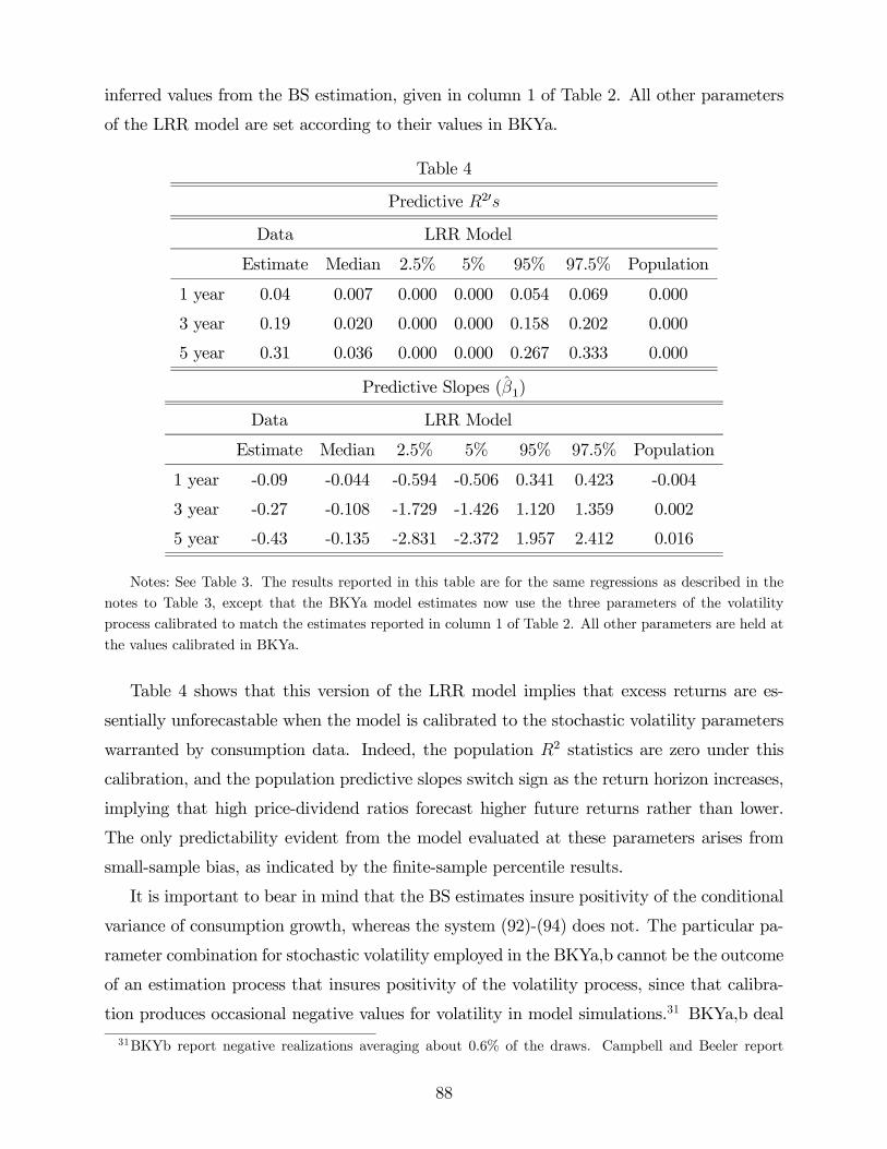
inferred values from the BS estimation, given in column 1 of Table 2. All other parameters

of the LRR model are set according to their values in BKYa.

Table 4

Predictive 20

Data LRR Model

Estimate Median 2.5% 5% 95% 97.5% Population

1 year 0.04 0.007 0.000 0.000 0.054 0.069 0.000

3 year 0.19 0.020 0.000 0.000 0.158 0.202 0.000

5 year 0.31 0.036 0.000 0.000 0.267 0.333 0.000

Predictive Slopes (1)

Data LRR Model

Estimate Median 2.5% 5% 95% 97.5% Population

1 year -0.09 -0.044 -0.594 -0.506 0.341 0.423 -0.004

3 year -0.27 -0.108 -1.729 -1.426 1.120 1.359 0.002

5 year -0.43 -0.135 -2.831 -2.372 1.957 2.412 0.016

Notes: See Table 3. The results reported in this table are for the same regressions as described in the

notes to Table 3, except that the BKYa model estimates now use the three parameters of the volatility

process calibrated to match the estimates reported in column 1 of Table 2. All other parameters are held at

the values calibrated in BKYa.

Table 4 shows that this version of the LRR model implies that excess returns are es-

sentially unforecastable when the model is calibrated to the stochastic volatility parameters

warranted by consumption data. Indeed, the population 2 statistics are zero under this

calibration, and the population predictive slopes switch sign as the return horizon increases,

implying that high price-dividend ratios forecast higher future returns rather than lower.

The only predictability evident from the model evaluated at these parameters arises from

small-sample bias, as indicated by the finite-sample percentile results.

It is important to bear in mind that the BS estimates insure positivity of the conditional

variance of consumption growth, whereas the system (92)-(94) does not. The particular pa-

rameter combination for stochastic volatility employed in the BKYa,b cannot be the outcome

of an estimation process that insures positivity of the volatility process, since that calibra-

tion produces occasional negative values for volatility in model simulations.31 BKYa,b deal

31BKYb report negative realizations averaging about 0.6% of the draws. Campbell and Beeler report

88

with this by discarding negative realizations and replacing them with small positive num-

bers. But when we instead infer the volatility parameters from the BS estimates rather than

calibrating them, we find that the persistence of the (inferred) monthly volatility process

in (92)-(94) can only be so high, for a given mean and volatility of the volatility process,

as a result of the requirement that volatility always be positive. Specifically, if we look at

the different percentiles of the posterior distribution for the parameters (89)-(91) reported

by BS (not shown), none of the estimated parameter combinations at any percentile deliver

the combination of and assumed in the BKYa,b calibration. Since those parameters

imply negative realizations and since the estimated values rule out negative realizations, this

is not possible.

Before concluding this section, it is worth making two further observations about the

evidence for changing volatility in consumption growth. First, there appears to be evidence

for large but highly infrequent shifts in the volatility of consumption growth, a phenomenon

that can have significant implications for the unconditional equity premium (Lettau, Lud-

vigson, and Wachter (2008)). Econometric models of changing volatility such as stochastic

volatility and GARCH-related processes are useful for describing higher frequency, station-

ary fluctuations in variance, but may be less appropriate for describing very infrequent,

prolonged shifts to a period of moderated volatility like that observed at the end of the last

century (the so-called Great Moderation). For example, GARCH models do not generate

the observed magnitude of volatility decline during the Great Moderation. Intuitively, these

models do a reasonable job of modelling changes in volatility within regimes, once those have

been identified by other procedures, but may not adequately capture infrequent movements

in volatility across regimes.

Second, the estimates of stochastic volatility obtained by Bidder and Smith were con-

ducted on post-war data, whereas most of the calibrations in the LRR literature are designed

to match data that include the pre-war period. The data sampling period is likely to play a

role in volatility estimates because pre-war consumption data are more volatile than post-war

data. While some of this difference may be attributable to a genuine difference in the volatil-

ity of fundamentals across the two periods, we also know that pre-war data are measured

with substantially more error than are post-war data, a fact that adds to the standard devia-

tion of measured consumption growth in samples that include pre-war data. Data collection

finding negative realizations 1.3% of the time using the same calibration, implying that when simulating 77

year paths for volatility using the BKYa,b calibration, over half go negative at some point.

89

methodologies changed discretely at the beginning of the post-war period, and Romer (1989)

finds that prewar GDP estimates significantly exaggerate the size of cyclical fluctuations in

the pre-war era. These considerations suggest that it may be prudent to restrict estimates

of consumption volatility to data from the post-war period, as Bidder and Smith do. On the

other hand, it is worth noting that the inferred parameter value governing the volatility of

volatility from the Bidder-Smith estimation (, in the first column of Table 2) is roughly

the same and if anything slightly larger than the calibrated value for this parameter in BKYa

and BKYb. This may be because the Bidder-Smith data include the recession of 2008-2010,

a time of unusually high consumption growth volatility in the post-war period.

In summary, the results in this section suggest that although there is evidence for a sizable

degree of stochastic volatility in aggregate consumption data, the magnitude of stochastic

volatility appears to be too small to be consistent with a non-negligible degree of time-

variation in the equity risk premium of currently calibrated LRR models. To the extent that

we seek to explain this aspect of the data, more work is needed to assess how the model can

be modified to generate an equity risk premium that is not only high on average, but also

significantly time-varying.

8 Asset Pricing with Habits

A prominent competing explanation for aggregate stock market behavior implies that assets

are priced as if there were a representative investor whose utility is a power function of the

difference between aggregate consumption and a habit level.32 In all of these theories, the

habit function is central part to the definition of risk, but there is substantial divergence

across models in how the habit stock is specified to vary with aggregate consumption. Some

work specifies the habit stock as a linear function of past consumption (e.g., Sundaresan

(1989); Constantinides (1990); Heaton (1995); Jermann (1998); Boldrin, Christiano, and

Fisher (2001)). More recent theoretical work often takes as a starting point the particular

nonlinear habit specification that includes current consumption developed in Campbell and

Cochrane (1999) (e.g., Campbell and Cochrane (2000); Li (2001); Wachter (2006); and Men-

32See Sundaresan (1989), Constantinides (1990), Ferson and Harvey (1992), Heaton (1995), Jermann

(1998), Campbell and Cochrane (1999), Campbell and Cochrane (2000); Boldrin, Christiano, and Fisher

(2001), Li (2001), Shore and White (2002); Dai (2003); Menzly, Santos, and Veronesi (2004); Wachter

(2006). Habit formation has also become an important feature of many dynamic macroeconomic models

as in An and Schorfheide (2007), Del Negro, Schorfheide, Smets, and Wouters (2007), Fernández-Villaverde

and Rubio-Ramírez (2007).

90

zly, Santos, and Veronesi (2004)). Moreover, there is no theoretical reason why other forms

of nonlinearities could not be entertained. Disagreement over the appropriate functional

form for the habit complicates estimation and testing of habit-based asset pricing models

because it implies that the functional form of the habit should be treated, not as known, but

rather as part and parcel of the estimation procedure.

There are at least three possible approaches to estimating and testing these models econo-

metrically, akin to those discussed above for estimating models with recursive preferences.

One is to estimate an explicit parametric model of the habit function, while leaving the

law of motion for consumption and other variables unspecified. Important early applica-

tions of this approach include Ferson and Constantinides (1991) and Heaton (1995) who use

distribution-free estimation procedures such as GMM to estimate habit- and durability-based

asset pricing models, where the habit is restricted to have a linear functional form. A second

approach is to estimate an entire parametric asset pricing model that embeds habit-formation

preferences. This parametric model includes not only a specification for the habit function,

but also a law of motion for the driving variables such as consumption and dividends. This

is done in BGT who use the same simulated method of moments approach discussed above

to estimate the Campbell and Cochrane (1999) habit model. A third approach is to evaluate

a general class of habit-based asset pricing models, placing as few restrictions as possible on

the specification of the habit function and no parametric restrictions on the law of motion

for consumption. This approach is taken in Chen and Ludvigson (2009), who treat the func-

tional form of the habit as unknown, and to estimate it nonparametrically along with the

rest of the model’s finite dimensional parameters.

An important distinction in this literature concerns the difference between “internal”

and “external” habit formation. About half of the theoretical studies cited at the beginning

of this section investigate models of internal habit formation, in which the habit is a func-

tion of the agent’s own past consumption. The other studies investigate models of external

habit formation, in which the habit depends on the consumption of some exterior reference

group, typically per capita aggregate consumption. Abel (1990) calls external habit forma-

tion “catching up with the Joneses.” Determining which form of habit formation is more

empirically plausible is important because the two specifications can have dramatically dif-

ferent implications for optimal tax policy and welfare analysis (Ljungqvist and Uhlig (2000)),

and for whether habit models can explain long-standing asset-allocation puzzles in the in-

ternational finance literature (Shore and White (2002)). Empirical tests allow us to assess

91

which variant of habit-formation is more likely to explain the data. I now describe how such

models may be estimated.

Consider a model of investor behavior in which utility is a power function of the difference

between aggregate consumption and the habit. Here I do not consider models in which utility

is a power function of the ratio of consumption to the habit stock, as in Abel (1990) and

Abel (1999). Ratio models of external habit formation imply that relative risk-aversion is

constant, hence they have difficulty accounting for the predictability of excess stock returns

documented in the empirical asset pricing literature. By contrast, difference models can

generate time-variation in the equilibrium risk-premium because relative risk aversion varies

countercyclically in these specifications.

Most approaches assume that identical agents maximize a utility function taking the

form

=

∞X=0

( −)

1− − 11−

(100)

Here is the level of the habit, and is the subjective time discount factor. is assumed

to be a function (known to the agent but unknown to the econometrician) of current and

past consumption

= ( −1 −)

such that ≥ 0 The function is quite general: the maximum lag length could

be infinity. This specification allows the habit to potentially depend on contemporaneous as

well as past consumption, a modeling choice that is a feature of several habit models in the

recent theoretical literature (e.g., Campbell and Cochrane (1999)).

When the habit is internal, the agent takes into account the impact of today’s con-

sumption decisions on future habit levels. In this case the intertemporal marginal rate of

substitution in consumption is given by

+1 = +1

(101)

where

=

= ( −)− −

"X=0

(+ −+)− +

# (102)

When the habit is external, agents maximize (100) but ignore the impact of today’s

consumption on tomorrow’s habits. In this case, the habit merely plays the role of an

92

externality and only the first term on the right-hand-side of (102) is part of marginal utility:

=

= ( −)−

In equilibrium, identical individuals choose the same consumption, so that regardless of

whether the habit is external or internal, individual consumption, , is equal to aggregate

per capita consumption, , which is simply denoted from now on.

8.1 Structural Estimation of Campbell-Cochrane Habit

BGT estimate the Campbell and Cochrane (1999) (CC) habit model, using the same simu-

lation approach discussed above to estimate the LRR model. An important aspect of their

approach is that the same moments and same observation equation that were used to evaluate

the LRR model are used to evaluate the Campbell-Cochrane model. BGT follow Campbell

and Cochrane’s model exactly except that they impose cointegration between consumption

and dividends. This changes the estimation only in so far as it changes the specification

of the model for the pricing kernel and for cash-flow dynamics. In particular, the CC

specification for cash-flows is assumed to be

∆+1 = + +1 (103)

∆+1 = + + +1 (104)

= ( − ) + − (105)

+1 +1 ∼ (0 1) (106)

Notice that the specification contains no long-run risk component in consumption growth,

or stochastic consumption volatility.

The external habit preferences imply a stochastic discount factor taking the form

+1 =

µ+1

+1

¶− ≡ −

where is referred to as the “surplus consumption ratio”. BGT follow CC and specify a

93

process for ln = as heteroskedastic and persistent:

+1 = (1− )+ + () +1

where and are primitive parameters and where

() =

½ 1

q1− 2 ¡ −

¢ ≤ max

0 max

The remaining parameters are defined by the Campbell-Cochrane model as

≡

r

1−

max ≡ +1

2

h1− ¡¢2i

Campbell and Cochrane (1999) provide a detailed explanation of the motivation behind

this specification. In particular, it delivers a slow moving habit that drives risk-premia and

long-horizon predictability of excess stock returns while maintaining a constant risk-free rate.

With this specification for+1 and cash-flow dynamics, the BGT procedure can be applied

in the same manner as described above for the LRR model. Notice that the procedure is

again fully structural in that it imposes a specific functional form for the habit function, as

well as a specification of the law of motion for the driving variables (103)-(106). I discuss

results below.

8.2 Flexible Estimation of Habit Preferences with Unrestricted

Dynamics

Another approach to estimating more general classes of habit models is to employ procedures

that place as few restrictions as possible on the specification of the habit function and no

parametric restrictions on the law of motion for consumption. This is reasonable if we want

to evaluate the idea that habits may be important, even if the specific functional forms

assumed in particular models are incorrect.

This section discusses Chen and Ludvigson (2009) who take this type of approach by

letting the data dictate the functional form of the habit function while employing an esti-

mation procedure that leaves the law of motion for the data unspecified. The objective is to

94

evaluates a general class of habit-based asset pricing models, placing as few restrictions as

possible on the specification of the habit and no parametric restrictions on the law of motion

for consumption. As in the application of EZW utility discussed above (Chen, Favilukis, and

Ludvigson (2007)), estimation and testing are conducted by applying the Sieve Minimum

Distance procedure to a set of Euler equations corresponding to the habit-based framework.

In this case the sieve part of the SMD procedure requires that the unknown function em-

bedded in the Euler equations (here the habit function) be approximated by a sequence of

flexible parametric functions.

Using stationary quarterly data on consumption growth, assets returns and instruments,

Chen and Ludvigson (CL) apply the SMD procedure to estimate all the unknown para-

meters of interest in the Euler equations underlying the optimal consumption choice of an

investor with access to asset payoffs. In addition to being robust to misspecification of

the functional form of the habit and the law of motion for the underlying fundamentals, the

SMD procedure estimates the unknown habit function consistently at some nonparametric

rate. The procedure also provides estimates of the finite dimensional parameters, here the

curvature of the power utility function and the subjective time-discount factor; these esti-

mates converge at rate√ (where is the sample size) and are asymptotically normally

distributed.

The asset pricing model estimated by CL comes from the first-order conditions for optimal

consumption choice for an investor with access to asset returns:

∙+1

+1

¸= 1 = 1 (107)

Referring back to (102), we see that the resulting equations yield a set of conditional

moment restrictions containing a vector of unknown parameters, ( )0, and a single unknown

habit function = ( −1 −).

Since consumption is trending over time, it is necessary to transform the model to use

stationary observations on consumption growth. CL address this problem by assuming that

the unknown habit function = ( −1 −) can be written as

=

µ−1

−

¶ (108)

where : R → R is an unknown function of the gross growth rates of consumption, with

domain space reduced by one dimension relative to . Note that now replaces as the

95

unknown function to be estimated along with ( ) using the Euler equations (107) and

the SMD procedure. As shown below, this assumption allows one to express the stochas-

tic discount factor, +1, as a function of gross growth rates in consumption, which are

plausibly stationary. One way to motivate (108) is to presume that the original function

= ( −1 −) is homogeneous of degree one, which allows the function to be

re-written as

=

µ1−1

−

¶ (109)

and redefined as in (108). The homogeneous of degree one assumption is consistent with

the habit models studied in the asset pricing literature cited above, including the nonlinear

habit specification investigated in Campbell and Cochrane (1999).

When the habit stock is a homogeneous of degree one function of current and past

consumption, marginal utility, , takes the form

= −

µ1−

µ−1

−

¶¶−(110)

−−

"X=0

µ+

¶− µ1−

µ+−1+

+−+

¶¶−+

#

where,

+

=

⎧⎪⎪⎪⎨⎪⎪⎪⎩

³+−1+

+−+

´∀ 6= 0

³−1

−

´−P

=1

³−1

−

´−

= 0

(111)

In the expression directly above, denotes the derivative of with respect to its −thargument.

To obtain an estimable expression for the unknown parameters of interest α = ( )0,

the Euler equations (107) must be rearranged so that the conditional expectation (·) ap-pears only on the outside of the conditional moment restrictions. Their are several equivalent

expressions of this form; here I present one. Denote the true values of the parameters with

an “” subscript: α = ( )0. Combining (110) and (107), and rearranging terms, we

find a set of conditional moment conditions:

(Ã

µ+1

¶−z+1+1 − 1

!Φ+1

)= 0 = 1 (112)

96

where

z+1 ≡

⎛⎜⎝³1−

³+1

+1−+1

´´−−∙P

=0

³+1++1

´− ³1−

³++1+

++1−+1+

´´− +1+

+1

¸ ⎞⎟⎠ Φ+1

Φ+1 ≡

⎛⎜⎝³1−

³−1

−

´´−−∙P

=0

³+

´− ³1−

³+−1+

+−+

´´− +

¸ ⎞⎟⎠

We may write (112) more compactly as

{(z+1 )|w∗ } = 0 = 1 (113)

where z+1 is a vector containing all observations used to estimate the conditional moment

(112) at time , is defined as

(z+1 ) ≡Ã

µ+1

¶−z+1+1 − 1

!Φ+1

and the conditional expectation in (57) is taken with respect to agents’ information set at

time , denoted w∗ .

Let w be a × 1 observable subset of w∗ that does not contain a constant. Equation(57) implies

{(z+1 )|w} = 0 = 1 (114)

Given the theoretical restrictions implied by (114), the rest of the procedure is similar

to that described above for the EZW estimation in CFL. The econometric model is again

semiparametric, in the sense that it contains both finite and infinite dimensional parameters

to be estimated.

8.3 Econometric Findings

BGT apply the simulated method of moments procedure to estimate and test the CC model

using the same observation equation and moments (defined by score functions) used to

evaluate the LRRmodel. An advantage of this approach is that the Chi-Squared specification

tests are comparable across models. BGT find that the Campbell-Cochrane specification is

not rejected, according to this 2 criterion. The persistence of the log surplus consumption

97

ratio, is close to unity, as in the Campbell and Cochrane (1999) calibration, and the

curvature parameter is precisely estimated and close to 0.84, somewhat lower than the

value of = 2 in their calibration. BGT conduct a number of other tests in order to

contrast their estimated versions of the LRR model and the CC habit model.

For most of these tests, BGT find that the estimated CC habit model and the estimated

LRR model have very similar implications. They both imply about the same fraction of

variability in the price-dividend ratio that is attributable to expected returns versus expected

dividend growth rates. They find about the same degree of forecastability of consumption

growth and dividend growth by the consumption-wealth ratios of each estimated model.

And they find about the same degree of forecastability of the long-horizon stock return by

the log dividend-price ratio. On one dimension they find clearer differences: estimates of a

consumption beta (formed from regressions of returns on consumption growth) model are

high in the habit model, about 4.19, whereas they are much lower, equal to 0.52, in the

LRR model. These values are computed from simulations of each model at the estimated

parameter values. The same consumption beta parameter estimated from the data is 0.79.

Turning to the semiparametric approach, CL estimate all the unknown parameters of

the flexible habit asset pricing model, and conduct statistical tests of hypotheses regarding

the functional form of the unknown habit as well as statistical tests for whether an internal

habit versus external habit specification better describes the data. The empirical results

suggest that the habit is a substantial fraction of current consumption—about 97 percent on

average—echoing the specification of Campbell and Cochrane (1999) in which the steady-state

habit-consumption ratio exceeds 94 percent.

CL find that the SMD estimated habit function is concave and generates positive in-

tertemporal marginal rate of substitution in consumption. The SMD estimated subjective

time-discount factor about 0.99. The estimated power utility curvature parameter is esti-

mated to be about 0.80 for three different combinations of instruments and asset returns, a

value that is remarkably similar to that found by BGT in the estimation of the Campbell-

Cochrane model. CL also develop a statistical test of the hypothesis of linearity and find

that the functional form of the habit is better described as nonlinear rather than linear. To

address the issue of external versus internal habit, CL derive a conditional moment restric-

tion that nests the internal and external nonlinear habit function, under the assumption that

both functions are specified over current and lagged consumption with the same finite lag

length. The empirical results indicate that the data are better described by internal habit

98

formation than external habit formation.

Finally, CL compare the estimated habit model’s ability to fit a cross-section of equity

returns with that of other asset pricing models, both quantitatively and in formal statis-

tical terms using the White reality check method discussed above. CL evaluate the SMD-

estimated habit model and several competing asset pricing models by employing the model

comparison distance metrics recommended in Hansen and Jagannathan (1997) (the so-called

HJ distance and the HJ+ distance), where all the models are treated as SDF proxies to the

unknown truth. In particular, the SMD-estimated internal habit model is compared to (i)

the SMD-estimated external habit model, (ii) the three-factor asset pricing model of Fama

and French (1993), (iii) the “scaled” consumption Capital Asset Pricing Model (CAPM) of

Lettau and Ludvigson (2001b), (iv) the classic CAPM of Sharpe (1964) and Lintner (1965),

and (v) the classic consumption CAPM of Breeden (1979) and Breeden and Litzenberger

(1978). Doing so, they find that a SMD-estimated internal habit model can better explain

a cross-section of size and book-market sorted equity returns, both economically and in a

statistically significant way, than the other five competing models.

8.4 Debate

BGT and BKYb provide evidence directly challenging the Campbell Cochrane habit model.

As noted above, BGT estimate consumption betas for both the CC habit model and the

LRR model and find that the beta of the latter is much closer to the beta in the data. The

reason for this difference is that the compensation for short-term consumption risk is small in

the LRR model, because most of the risk premium is generated by the long-run component

. This leads to a small consumption beta, more in line with the data.

BKYb further argue that the data provide little evidence of forecastability of price-

dividend ratios by contemporaneous consumption growth, consistent with the LRR model.

This is because the LRR model’s state variables are expectations of future consumption

growth and volatility. They emphasize that the Campbell-Cochrane habit model generates a

backward looking state variable for asset prices that implies strong forecastability of future

price-dividend ratios by current consumption growth rates. BGT report a similar finding:

in the estimated Campbell-Cochrane habit model the log price-dividend ratio is related to

both current and lagged consumption growth, whereas there is little such relation in the data.

These results suggest that the Campbell-Cochrane habit model implies too much correlation

between asset prices and past consumption values.

99

Brunnermeier and Nagel (2008) question habit formation from a different perspective.

They note that those habit formation models that generate time-varying risk aversion imply

that, as liquid wealth increases, agents become less risk averse and therefore should invest

proportionally more in risky assets such as stocks. Using data from the Panel Study of In-

come Dynamics, they study how households’ portfolio allocation decisions change with liquid

wealth. They find little relation between the two for households who already participate in

the stock market. This evidence is important because it is directed at the key channel for

generating time-varying risk-premia in habit models: fluctuations in risk-aversion, which in

turn generate fluctuations in the demand for risky securities. The household data studied

by Brunnermeier and Nagel (2008) apparently provides little support for this mechanism.

9 Asset Pricing With Heterogeneous Consumers and

Limited Stock Market Participation

So far we have been studying theories in which the pricing kernel is specified as a function

of the consumption of a representative agent for some group, typically all households in

the economy. In these models agents are either identical or any heterogeneous risks are

perfectly insurable, so that assets can be priced as if there were a representative investor

who consumed the per capita aggregate expenditure level.

A separate strand of the literature has argued that asset prices are determined by the be-

havior of heterogeneous agents, and that this heterogeneity plays a role in the pricing kernel.

Constantinides and Duffie (1996) demonstrate a set of theoretical propositions showing that,

when markets are incomplete (so that heterogeneous shocks are not perfectly insurable), any

observed joint process of aggregate consumption and returns can be an equilibrium outcome

if the second moments of the cross-sectional distribution of consumption growth and asset

returns covary in the right way. In particular, the model can explain a higher equity premium

and Sharpe ratio with lower risk aversion than the complete markets (representative agent)

counterpart if the cross-sectional variance of consumption is countercyclical and negatively

related to aggregate consumption growth.33 Others have emphasized that not everyone owns

stocks, and that stock prices are determined by stockholders. Researchers have explored the

role of limited stock market participation in explaining stock return data (Mankiw and Zeldes

(1991), Vissing-Jorgensen (2002), Guvenen (2003)).

33Mankiw (1986) makes the same point in a simpler theoretical model.

100

Because the estimation and testing of incomplete markets and/or limited participation

models requires disaggregated, household-level data that often has a short time-series di-

mension and is subject to significant measurement error, the literature has progressed slowly

in evaluating these models empirically relative to the representative agent formulations dis-

cussed above. I discuss the findings of a few studies here, and note the importance of future

research as more and better data are amassed.

Using household level income data, Storesletten, Telmer, and Yaron (2004) found strong

evidence of countercyclical variation in idiosyncratic income risk. Because households’ can

save, this is not the same as countercyclical variation in individual consumption risk, some-

thing required by heterogeneous-agent models if they are to improve upon the asset pricing

implications of their representative agent counterparts. For example, in the heterogeneous

agent model of (Constantinides and Duffie (1996)), in order to explain the equity premium

with lower risk aversion than its representative agent counterpart, the conditional variance

of idiosyncratic consumption risk must vary inversely with the aggregate stock market, so

that equities are an unattractive form of precautionary wealth.

To investigate the importance of heterogeneity in driving asset prices, several studies have

estimated models on household-level consumption data using the Consumer Expenditure

Survey (CEX). Because this survey has a limited panel element, researchers have instead

focused on the cross-sectional implications of the model.

Brav, Constantinides, and Geczy (2002), Cogley (2002) and Vissing-Jorgensen (2002)

derive representations of the model that rely only on cross-sectional moments of consumption

growth. To see how this may be accomplished, consider households indexed by . Let

denote the log growth rate in household ’s consumption, :

≡ log (−1)

Denote also the intertemporal marginal rate of substitution (MRS) in consumption as

= ()

With power utility, the MRS is

() = exp (−)

101

>From the first-order condition for optimal consumption choice, the Euler equation holds

for each household

[ (+1) (+1)] = 1 = 1 ; = 1 (115)

This implies that the MRS of any household is a valid stochastic discount factor. Since

any household’s MRS is a valid stochastic discount factor, so is the average MRS across

households. Thus, we may take cross-sectional average of (115), to derive no-arbitrage

restrictions for the th traded asset return taking the form

"Ã1

X=1

(+1)

!+1

#= 1 (116)

Using the law of iterated expectations, (116) holds unconditionally

"Ã1

X=1

(+1)

!(1 ++1)

#= 1 (117)

The formulations in (116) or (117) are useful because they allow for the use of repeated

cross-sections when empirically evaluating the model. This is important if the household

level data have, as they do, a limited panel dimension with a short time-series element.

Brav, Constantinides, and Geczy (2002) point out that (116) and (117) are still subject

to measurement error because, under power utility, each term in the sum 1

P

=1 (+1)

is (+1)−

These terms are raised to a large power if the coefficient is high,

implying that a small amount of measurement error in can lead to a large amount of

specification error in the econometric asset pricing model. It is therefore useful to consider

a Taylor series expansion of the pricing kernel in (116). Brav, Constantinides, and Geczy

(2002), and Cogley (2002) approximate () with a third-order polynomial in . Let

denote the cross-sectional mean consumption growth at time

≡1

X=1

Expanding around delivers

() ≈ ()+0 () ( − )+(12)

00 () ( − )2+(16) 000 () ( − )

3

102

Taking the cross-sectional average of this expanded pricing kernel at each date leads to

1

X=1

(+1) ≈ () + (12)00 ()2 + (16)

000 ()3

where 2 and 3 denote the second and third cross-sectional moments of consumption

growth, respectively:

2 =1

X=1

( − )2

3 =1

X=1

( − )3

Under complete markets, agents equate their intertemporal marginal rates of substitution

in consumption state-by-state, so that higher order cross-sectional moments other than the

first do not enter the pricing kernel and do not matter for asset prices.

Brav, Constantinides, and Geczy (2002), Cogley (2002) and Vissing-Jorgensen (2002)

focus on specifications with power utility,

() = exp (−)

implying

1

X=1

() ≈ exp (−)£1 +

¡22

¢2 −

¡36

¢3¤ (118)

Denote the third-order expanded pricing kernel based on (118) as f:

f+1 ≡ exp (−)£1 +

¡22

¢2 −

¡36

¢3¤ (119)

Risk-premia in this model depend on cov(e+1 +1) which equals

cov (e+1 +1) = cov¡log¡ exp

¡−+1¢ £1 + ¡22¢2+1 − ¡36¢3+1¤¢ +1¢ (120)

An asset is risky when cov (e+1 +1) 0 and it provides insurance when cov (e+1 +1)

0. Equation (120) implies assets that covary positively with cross-sectional consumption

variance (across groups) and/or negatively with cross-sectional skewness will have lower

risk-premia than assets that covary negatively (or less positively) with cross-sectional con-

103

sumption variance and/or positively (or less negatively) with skewness. Intuitively, returns

that covary negatively with cross-sectional consumption inequality are risky because they

unattractive as a store of precautionary balances: they pay off poorly when idiosyncratic

consumption risk is high.

Brav, Constantinides, and Geczy (2002), Cogley (2002) estimate nonlinear Euler equa-

tions [+1+1] = 1 using estimates of (119) from the CEX along with data on aggregate

equity returns. Their objective is to assess whether the models are able to account for the

observed equity premium, at lower levels of risk aversion, than the complete markets coun-

terpart where the higher-order cross-sectional moments play no role in the pricing kernel.

Vissing-Jorgensen (2002) estimates a log-linearized version of the conditional Euler equation,

conditional on time information. She focuses on estimating the parameter .

Vissing-Jorgensen (2002) reports findings for −1, which she interprets as an estimate only

of the EIS, rather than the inverse of risk-aversion. She points out that if preferences are

not of the power utility form but are instead of the EZW form, estimation of the conditional

log-linearized Euler equation, which involves a regression of consumption growth onto log

asset returns, provides an estimate of the EIS but is not informative about risk-aversion. She

notes that the Euler equation should hold for a given household only if that household holds a

nonzero position in the asset so that including the consumption of non-asset holders in Euler

equation estimates will lead to inconsistent estimates of the EIS, which will be downward

biased when the consumption growth of nonasset holders does not covary with predictable

return movements at all. Distinguishing between assetholders and non-assetholders using the

CEX, she finds estimates of the EIS that are larger than those obtained in some estimates

using aggregate data, equal to 0.3-0.4 for stockholders and 0.08-1.0 for bondholders. But she

also finds that her results are largely unchanged using a pricing kernel comprised of per-capita

average consumption of stockholders, suggesting that what matters most for her findings is

the stockholder status distinction, rather than the higher-order cross-sectional moments of

consumption that are a feature of the pricing kernel when markets are incomplete.

Brav, Constantinides, and Geczy (2002), and Cogley (2002) investigate the same data

but reach different conclusions. Brav, Constantinides, and Geczy (2002) find that both the

average MRS across households, as appears in (116), as well as a third-order expansion of this

average, as appears in (119), are valid pricing kernels (the Euler equation restrictions are not

rejected using these kernels), and both kernels are able to explain all of the observed equity

premium with a coefficient of relative risk aversion of three or four. By contrast, Cogley

104

(2002) finds that the pricing kernel based on the third-order expansion can only explain about

a third of the observed equity premium when the coefficient of relative risk aversion is less

than 5. In a separate result, Brav, Constantinides, and Geczy (2002) explore representative

stockholder versions of the pricing kernel, where the SDF is expressed in terms of the per

capita average growth rate for stockholders who report a certain threshold of assets owned.

This is different from the approach described above because the pricing kernel here depends

on the growth in mean consumption for anyone classified as an assetholder, rather than mean

of consumption growth across all households. They find that, for threshold-wealth values

between $20,000 and $40,000, the representative stockholder version of the model explains

the equity premium for values of RRA between 10 and 15.

It is unclear what the reasons are for the difference in results reported in Brav, Constan-

tinides, and Geczy (2002), and Cogley (2002), but there are at least two possibilities. First,

the two studies use different samples. Brav, Constantinides, and Geczy (2002) use a sample

that covers the period from the first quarter of 1982 to the first quarter of 1996. Cogley

(2002) uses a sample that runs from the second quarter of 1980 through the fourth quarter of

1994. Second, the papers employ different ways of dealing with measurement error. In par-

ticular, Brav, Constantinides, and Geczy (2002) assume multiplicative measurement error in

the level of consumption and trim the sample of outliers in household consumption growth.

Cogley (2002) assumes additive measurement error in the growth of consumption and makes

an analytical adjustment to the equity premium estimates to account for this error, but does

not trim the sample. Brav, Constantinides, and Geczy (2002) attempt to mitigate mea-

surement error by deleting a household’s consumption growth if the increase in this growth

from one quarter to the next is greater than a certain threshold (if −1 12 and

+1 2), and they delete any consumption growth if it is greater than five. Both

studies delete households for which there is no information in consecutive quarters about

consumption. These considerations suggest that results may be sensitive to the treatment

of measurement error.

To mitigate measurement error, a number of recent papers have sought different ap-

proaches to aggregating the Euler equations of individual households. For example, instead

of taking cross-sectional averages of (115), which results in a pricing kernel that is the equally

105

weighted average of household marginal rates of substitution

+1 =1

X=1

µ+1

¶− (121)

one could take cross-sectional averages of both sides of

()− =

£

−+1+1

¤

resulting in

1 =

"

1

P

=1−+1

1

P

=1−

+1

#and implying a pricing kernel taking the form

=1 =

1

P

=1−+1

1

P

=1−

(122)

The kernel above is the ratio of average marginal utilities rather than the average of the

ratio of marginal utilities. Balduzzi and Yao (2007), Kocherlakota and Pistaferri (2009), and

Semenov (2010) use pricing kernels of this form.

Kocherlakota and Pistaferri (2009) argue that (122) is less subject to measurement error

than (121) because, if there is stationary multiplicative measurement error in the level of

consumption, so that measured consumption ∗ = exp () then (121) is equal to the

true average MRS discount factor multiplied times a constant, whereas (122) is unaffected

by this form of measurement error as long as is stationary and exp (−) ∞.34 Noticehowever, that measurement error of this form cannot explain the conflicting results in Brav,

Constantinides, and Geczy (2002) and (Cogley (2002)), because the kernel (121) used in

these papers differs from the true average only by a constant. It is therefore still a valid

pricing kernel for return differentials like the equity premium even if it is invalid for the level

of returns.

Balduzzi and Yao (2007) use the CEX and find that a pricing kernel of the form (122)

can reduce the (annualized) unexplained equity premium to zero when = 10 whereas a

representative agent pricing kernel (equal to the MRS of per capita, aggregate CEX con-

34Kocherlakota and Pistaferri (2009) show that the measured version of (122) is the same as its theoretical

counterpart multiplied by the ratio (exp (−+1)) (exp (−)) Given stationarity of , this ratio isa finite constant as long as (exp (−)) is finite.

106

sumption) implies an unexplained premium of between 8% and 10% for the same level of

risk aversion. An RRA coefficient of 10 is higher than the values of 3 or 4 that Brav, Con-

stantinides, and Geczy (2002) found was required to explain the equity premium using the

third-order approximation to (121) as a pricing kernel. By contrast, Kocherlakota and Pista-

ferri (2009) find that a representative agent pricing kernel can explain all of the observed

equity premium if is around 58, but not if it is smaller, while there is no value of (positive

or negative) for which the pricing kernel (122) using CEX data is capable of explaining the

equity premium. It is again not clear why these results seem to differ so much, except to

note the different CEX samples used: Balduzzi and Yao (2007) study the period 1982-1995,

while Kocherlakota and Pistaferri (2009) study the period 1980-2004.

Kocherlakota and Pistaferri (2009) also study a different pricing kernel based on the idea

that the incomplete markets pricing kernel (122) may be too restrictive if in fact agents

have access to forms of insurance (such as government or informal social networks) against

idiosyncratic productivity shocks. They develop a pricing kernel that is valid in models

where agents have private information about their labor effort but a government provides

Pareto optimal allocations. This kernel differs from both the representative agent and the

incomplete markets kernel (122) and equals times the th moment of the cross-sectional

distribution of consumption at time to that at time + 1. They find that, for = 5, this

pricing kernel (estimated on CEX data) is able to explain all of the equity premium.

Finally, Semenov (2010) uses the CEX data to study a pricing kernel based on (122).

Instead of employing (122) directly, he takes a -th order Taylor expansion of the numerator

and denominator around average consumption. He uses the ratio of these linear expansions

as a pricing kernel and motivates its use by giving an empirical example under which the

resulting kernel is less subject to measurement error than is (122). He finds that this alter-

native kernel can explain the observed equity premium with a value for of three or lower,

especially as he restricts attention to households with higher wealth thresholds.

One aspect of these data that is not typically addressed is that the different sub-groups of

households, which differ according to whether a household is classified as a stockholder or not,

or by different wealth-threshold levels, contain different numbers of observations. They are

therefore subject to different degrees of measurement error. For example, there are far more

nonstockholders, according to any of the several methods for identifying stockholder status

typically employed, than there are stockholders in the CEX sample. This implies that the

consumption of stockholders (once aggregated) will be more subject to measurement error

107

than will be the consumption of nonstockholders and especially more subject to measurement

error than the per capita consumption of all households. For that reason alone, stockholder

consumption will be more volatile than nonstockholder consumption. It follows that, without

some adjustment for the heterogeneity in measurement error caused by different sample sizes,

the cross-sectional moments of consumption are not comparable across sub-groups.

To the best of my knowledge this has been addressed in only one paper, namely the

working paper version of Malloy, Moskowitz, and Vissing-Jorgensen (2009). These authors

provide a procedure for adjusting the consumption moments of different sub-groups for dif-

ferences in the size of the cross-section of each group. The adjustments matter substantially.

For example, without adjustments, the standard deviation of quarterly consumption growth

of stockholders is 0.034, or 4.9 times as volatile as quarterly aggregate consumption growth.

With adjustments, the standard deviation of quarterly stockholder consumption growth is

0.018, or 2.6 times as volatile as aggregate consumption. Future empirical work should

explicitly account for the differences in the size of the cross-section of each group when

comparing asset pricing results for different pricing kernels defined over the consumption of

different groups.

It is difficult to draw general conclusions from the results in this section. The mixed

results seem to depend sensitively on a number of factors, including the sample, the em-

pirical design, on the method for handling and modeling measurement error, the form of

cross-sectional aggregation of Euler equations across heterogeneous agents, and the imple-

mentation, if any, of linear approximation of the pricing kernel. A tedious but productive

task for future work will be to carefully control for all of these factors in a single empirical

study, so that researchers may better assess whether the household consumption hetero-

geneity we can measure in the data has the characteristics needed to explain asset return

data.

10 Conclusion

We have learned much from the progress made over the last 15 years in consumption-based

asset pricing. In contrast to the standard consumption-based model derived from a repre-

sentative agent with power utility preferences, we now have several reasonable frameworks

for understanding the high and time-varying equity market risk premium, the excess volatil-

ity of stock markets, and for better understanding the cross-sectional dispersion in average

108

returns. These findings and others have reinvigorated interest in consumption-based asset

pricing, spawning a new generation of leading consumption-based asset pricing theories.

As the large and growing body of empirical work summarized here indicates, none of

the models in this newer generation are likely to explain all features of the data. Tests of

scaled multifactor consumption-based models suggest that a pricing kernel that is an approx-

imately linear but state-dependent function of consumption growth performs substantially

better than a state-independent counterpart, but other results suggest that some theoretical

restrictions implied by these models may not be satisfied. Models with habits show promise

in explaining the dynamics of the equity premium and, in some studies, the cross-section

of average returns, but they also seem to imply too much correlation between stock market

valuation ratios and current and past consumption. Models with recursive preferences, when

combined with long-run consumption risk, do a better job of matching asset return data than

a counterpart without long-run risk and/or with power utility, but they also have difficulty

generating significant time-variation in the equity risk-premium, especially when parameters

of the stochastic consumption volatility process are calibrated to estimates warranted from

consumption data. Heterogeneity in stock market participation and in idiosyncratic risk

produces a far richer array of asset pricing implications than does the standard model, but

direct empirical tests of these models often lead to conflicting results. Finally, despite the

important progress these models represent, leading consumption-based theories (including

those based on habits, long-run risk, and/or limited stock market participation), often fail

to explain the mispricing of the standard model. This result implies that these models are

still missing an important feature of the data involving the joint dynamics of consumption

and asset returns.

For the most part, empirical analysis of these models has adhered to the long-standing

convention of employing statistical tests of the null of correct specification against the alter-

native of incorrect specification. I have argued here that asking whether a model is perfectly

specified is the wrong question, or at least not the only relevant question. All models are

abstractions of reality and the data we use to test them are measured with error. Misspec-

ified models may still offer central insights that help us interpret important aspects of the

data even if they don’t explain all aspects. How shall we judge models when we are prepared

to accept the premise that none are perfectly specified? One approach to this problem is to

focus on quantifying specification error and comparing this error across competing specifi-

cations, rather than focusing exclusively or primarily on testing whether individual models

109

are free of any specification error. This chapter discussed one such test that can be applied

across a range of asset pricing applications. More work is needed to develop procedures for

uncovering superior specifications that potentially combine elements from several models.

This chapter did not have space to cover the burgeoning literature on rare consumption

disasters as an explanation of stock market behavior. The formal empirical analysis of this

paradigm is in its infancy, if for no other reason that it is hard to make precise statistical

inferences from the very few (if any) data points in our sample that by definition represent

rare disasters. As a consequence, most recent work in this area is purely theoretical, in which

the probability of a disaster is calibrated to match certain features of asset return data, with-

out being informed by evidence on disasters in consumption data.35 An exception is Barro

(2006), who argues that it is possible to explain the equity premium in the standard model

with low risk aversion, once the probability of a disaster is calibrated to match international

data on large economic declines. Subsequent empirical studies have questioned the role of

rare events in explaining the equity premium, especially if agents are restricted to have low

risk-aversion.36

In the future researchers will almost certainly find increasingly creative ways to economet-

rically test the validity and performance of models with rare disasters as a primary feature.

However this empirical evidence turns out, the allowance for disasters in standard models of

risk provides an example of how superior specifications may potentially be obtained by com-

bining elements of several consumption-based models. An example of this approach can be

found in the work of Wachter (2010), who combines recursive preferences with a time-varying

probability of disaster. Time-varying disaster probabilities produce time-varying discount

rates, and therefore generate empirically plausible forecastability of the equity premium and

excess volatility of the stock market. The time-varying disaster probability thereby enhances

the ability of models with recursive preferences to explain these features of the data rela-

tive to the specifications discussed above. An important unresolved question is whether the

time-varying disaster probabilities we can measure empirically from consumption data have

35See for example Longstaff and Piazzesi (2004), Gourio (2008), Martin (2008), Gabaix (2009) and Wachter

(2010).36Backus, Chernov, and Martin (2010) use a macro-finance model to impute the distribution of consump-

tion growth from the observed behavior of options prices, which contain information about how market

participants view extreme events. They find smaller probabilities of extreme outcomes than what is es-

timated from the Barro international data. Julliard and Ghosh (2010) estimate the consumption Euler

equations of the standard model allowing explicitly for the probabilities attached to different states to differ

from their sample frequencies. They find the model is still rejected and requires a high level of risk aversion

to explain the equity premium.

110

the characteristics needed to explain these features of asset markets, and more.

111

References

Abel, A. B. (1990): “Asset Prices Under Habit Formation and Catching Up With the

Jones,” American Economic Review, 80, 38—42.

(1999): “Risk Premia and Term Premia in General Equilibrium,” Journal of Mon-

etary Economics, 43, 3—33.

Ai, C., and X. Chen (2007): “Estimation of Possibly Misspecified Semiparametric Con-

ditional Moment Restriction Models with Different Conditioning Variables,” Journal of

Econometrics, 141, 5—43.

Ai, H., M. M. Croce, and K. Li (2010): “Toward a Quantitative General Equilibrium

Asset Pricing Model with Intangible Capital,” Unpublished paper, UNC Kenan-Flagler

Business School.

Altonji, J. G., and L. M. Segal (1996): “Small-Sample Bias in GMM Estimation of

Covariance Structures,” Journal of Business and Economic Statistics, 14, 353—66.

An, S., and F. Schorfheide (2007): “Bayesian Analysis of DSGE Models,” Econometric

Reviews, 26(2-4), 113—172.

Andrieu, C., A. Doucet, and R. Holenstein (2010): “Particle Markov Chain Monet

Carlo with Discussion,” Journal of Royal Statistical Society Series B, 72, 269—342.

Ang, A., and G. Bekaert (2007): “Stock Return Predictability: Is it There?,” Review of

Financial Studies, 20(3), 651—707.

Anthony Smith, J. (1993): “Estimating Nonlinear Time-Series Models Using Simulated

Vector Autoregressions,” Journal of Applied Econometrics, 8, S63—S84.

Attanasio, O., and G. Weber (1989): “Intertemporal Substitution, Risk Aversion and

the Euler Equation for Consumption,” The Economic Journal, 99, 59—73.

Backus, D., M. Chernov, and I. Martin (2010): “Disasters Implied By Equity Index

Options,” Unpublished paper, New York University.

112

Balduzzi, P., and T. Yao (2007): “Testing Heterogeneous-agent Models: An Alternative

Aggregation Approach,” Journal of Monetary Economics, 54, 369—412.

Bansal, R., R. F. Dittmar, and D. Kiku (2009): “Cointegration and Consumption Risk

in Equity Returns,” Review of Financial Studies, 22, 1343—1375.

Bansal, R., R. F. Dittmar, and C. T. Lundblad (2005): “Consumption, Dividends,

and the Cross-Section of Equity Returns,” Journal of Finance, 60(4), 1639—1672.

Bansal, R., A. R. Gallant, and G. Tauchen (2007): “Rational Pessimism, Rational

Exuberance, and Asset Pricing Models,” Review of Economic Studies, 74, 1005—1033.

Bansal, R., D. Kiku, and A. Yaron (2007a): “A Note on the Economics and Statistics

of Predictability,” Unpublished paper, Fuqua School, Duke University.

(2007b): “Risks for the Long-Run: Estimation and Inference,” Unpublished paper,

Fuqua School, Duke University.

(2009): “Empirical Evaluation of the Long-Run Risks Model for Asset Prices,”

Unpublished paper, Fuqua School, Duke University.

Bansal, R., and A. Yaron (2004): “Risks for the Long-Run: A Potential Resolution of

Asset Pricing Puzzles,” Journal of Finance, 59(4), 1481—1509.

Barro, R. (2006): “Rare Disasters and Asset Markets in the Twentieth Century,” The

Quarterly Journal of Economics, pp. 823—866.

Beaudry, P., and E. van Wincoop (1996): “The Intertemporal Elasticity of Sustitution:

An Exploration Using a U.S. Panel of States,” Economica, 63(251), 495—512.

Bidder, R., and M. E. Smith (2010): “Doubts and Variability,” Unpublished working

paper, New York University.

Boldrin, M., L. J. Christiano, and J. D. M. Fisher (2001): “Habit Persistence, Asset

Returns and the Business Cycle,” American Economic Review, 91(1), 149—166.

Brav, A., G. M. Constantinides, and C. C. Geczy (2002): “Asset Pricing with Hetero-

geneous Consumers and Limited Participation: Empirical Evidence,” Journal of Political

Economy, 110(4), 793—824.

113

Breeden, D. (1979): “An Intertemporal Asset Pricing Model with Stochastic Consumption

and Investment Opportunities,” Journal of Financial Economics, 7, 265—296.

Breeden, D., M. Gibbons, and R. Litzenberger (1989): “Empirical Tests of the

Consumption-Oriented CAPM,” Journal of Finance, 44, 231—262.

Breeden, D., and R. Litzenberger (1978): “Prices of State-Contingent Claims Implicit

in Option Prices,” Journal of Business, 51, 621—651.

Brunnermeier, M., and S. Nagel (2008): “Do Wealth Fluctuations Generate Time-

Varying Risk Aversion? Micro-Evidence on Individuals’ Asset Allocation,” American

Economic Review, 98(3), 713—736.

Bui, M. P. (2007): “Long-run Risks and Long-run Predictability: A Comment,” Unpub-

lished paper, Harvard University.

Campbell, J. Y. (1993): “Intertemporal Asset Pricing Without Consumption Data,”

American Economic Review, 83, 487—512.

(1996): “Understanding Risk and Return,” Journal of Political Economy, 104(2),

298—345.

(2003): “Consumption-Based Asset Pricing,” in Handbook of the Economics of

Finance Vol. I-B, ed. by G. Constantinides, M. Harris, and R. Stulz, pp. 803—887. Elsevier

Science B.V., North Holland, Amsterdam.

Campbell, J. Y., and J. Beeler (2009): “The Long-Run Risks Model and Aggregate

Asset Prices: An Empirical Assessment,” Unpublished paper, Harvard University.

Campbell, J. Y., and J. H. Cochrane (1999): “By Force of Habit: A Consumption-

Based Explanation of Aggregate Stock Market Behavior,” Journal of Political Economy,

107, 205—251.

(2000): “Explaining the Poor Performance of Consumption-Based Asset Pricing

Models,” Journal of Finance, 55(6), 2863—2878.

Campbell, J. Y., A. W. Lo, and C. MacKinlay (1997): The Econometrics of Financial

Markets. Princeton University Press, Princeton, NJ.

114

Campbell, J. Y., and G. Mankiw (1989): “Consumption, Income, and Interest Rates:

Reinterpreting the Time Series Evidence,” in NBER Macroeconomics Annual: 1989, ed.

by O. Blanchard, and S. Fischer, pp. 185—216. MIT Press, Cambridge, MA.

Campbell, J. Y., C. Polk, and T. Voulteenaho (2005): “Growth or Glamour? Fun-

damentals and Systematic Risk in Stock Returns,” NBER Working Paper No. 11389.

Campbell, J. Y., and S. Thompson (2005): “Predicting the Equity Premium Out of

Sample: Can Anything Beat the Historical Average?,” NBER working paper No. 11468.

Campbell, J. Y., and L. Viceira (2001): Strategic Asset Allocation: Portfolio Choice for

Long-Term Investors. Oxford Univeristy Press, London, UK.

Chamberlain, G., and M. Rothschild (1983): “Arbitrage, Factor Structure, and Mean-

Variance Analysis on Large Asset Markets,” Econometrica, 51, 1281—1304.

Chen, X., J. Favilukis, and S. C. Ludvigson (2007): “An Estimation of Economic

Models with Recursive Preferences,” Unpublished paper, New York University.

Chen, X., and S. C. Ludvigson (2009): “Land of Addicts? An Empirical Investigation of

Habit-Based Asset Pricing Models,” Journal of Applied Econometrics, 24(7), 1057—1093.

Clark, T. (2009): “Is the Great Moderation Over? An Empirical Investigation,” Economic

Review, Federal Reserve Bank of Kansas City, pp. 5—42.

Cochrane, J. H. (1996): “A Cross-Sectional Test of an Investment-Base Asset Pricing

Model,” Journal of Political Economy, 104, 572—621.

(2005): Asset Pricing, Revised Edition. Princeton University Press, Princeton, NJ.

(2008): “The Dog That Did Not Bark: A Defense of Return Predictability,” Review

of Financial Studies, 21(4), 1533—1575.

Cogley, T. (2002): “Idiosyncratic Risk And The Equity Premium: Evidence From The

Consumer Expenditure Survey,” Journal of Monetary Economics, 49, 309—334.

Colacito, R., and M. M. Croce (2004): “Risks for the Long Run and the Real Exchange

Rate,” Unpublished paper, New York University.

115

Constantinides, G. M. (1990): “Habit-formation: A Resolution of the Equity Premium

Puzzle,” Journal of Political Economy, 98, 519—543.

Constantinides, G. M., and D. Duffie (1996): “Asset Pricing With Heterogeneous

Consumers,” Journal of Political Economy, 104, 219—40.

Constantinides, G. M., and A. Ghosh (2009): “The Cross-Section of Returns with

Regime Shifts in Consumption and Dividend Growth,” Unpublished paepr, University of

Chicago.

(2010a): “Asset Pricing Tests with Long-Run Risks in Consumption Growth,”

Unpublished paepr, University of Chicago.

(2010b): “The Predictability of Returns with Regime Shifts in Consumption and

Dividend Growth,” Unpublished paepr, University of Chicago.

Cornell, B. (1999): “Risk, Duration, and Capital Budgeting: New Evidence on Some Old

Questions,” The Journal of Business, 72, 183—200.

(2000): “Equity Duration, Growth Options and Asset Pricing,” The Journal of

Portfolio Management, 26, 105—111.

Creal, D. (2009): “A Survey of Sequential Monte Carlo Methods for Economics and Fi-

nance,” Unpublished paper, Booth School, University of Chicago.

Croce, M. M., M. Lettau, and S. C. Ludvigson (2010): “Investor Information, Long-

Run Risk and the Duration of Risky Cash Flows,” Unpublished paper, New York Univer-

sity.

Da, Z. (2005): “Cash Flow, Consumption Risk, and the Cross-Section of Stock Returns,”

Unpublished paper, Norwestern University.

Dai, Q. (2003): “Term Structure Dynamics in a Model with Stochastic Internal Habit,”

Unpublished paper, Stern School of Business, New York University.

Dechow, P. M., R. G. Sloan, and M. T. Soliman (2004): “Implied Equity Duration:

A New Measure of Equity Risk,” Review of Accounting Studies, 9, 197—228.

Del Negro, M., F. Schorfheide, F. Smets, and R. Wouters (2007): “On the Fit of

New Keynesian Models,” Journal of Business and Economic Statistics, 25(2), 123—162.

116

Duffee, G. R. (2005): “Time Variation in the Covariances Between Stock Returns and

Consumption Growth,” Journal of Finance, 60(4), 1673—1712.

Epstein, L., and S. Zin (1989): “Substitution Risk Aversion and the Temporal Behavior of

Consumption and Asset Returns: A Theoretical Framework,” Econometrica, 57, 937—968.

(1991): “Substitution, Risk Aversion, and the Temporal Behavior of Consumption

and Asset Returns: An Empirical Investigation,” Journal of Political Economy, 99, 555—

576.

Fama, E. F., and K. R. French (1992): “The Cross-Section of Expected Returns,”

Journal of Finance, 47, 427—465.

(1993): “Common Risk Factors in the Returns on Stocks and Bonds,” Journal of

Financial Economics, 33, 3—56.

Fama, E. F., and J. MacBeth (1973): “Risk, Return and Equilibrium: Empirical Tests,”

Journal of Political Economy, 81, 607—636.

Fernández-Villaverde, J., and J. F. Rubio-Ramírez (2007): “How Structural Are

Structural Parameters?,” in NBER Macroeconomics Annual: 2007, ed. by D. Acemoglu,

K. Rogoff, and M. Woodford, vol. 22. MIT Press, Cambridge, MA.

Ferson, W. E., and G. M. Constantinides (1991): “Habit Persistence and Durability

in Aggregate Consumption,” Journal of Financial Economics, 29, 199—240.

Ferson, W. E., and C. R. Harvey (1992): “Seasonality and Consumption-Based Asset

Pricing,” Journal of Finance, 47, 511—552.

Gabaix, X. (2009): “A Simple, Unified, Exactly Solved Framework For Ten Puzzles in

Macro-finance,” Unpublished paper, New York University.

Gallant, A. R., and G. Tauchen (1989): “Seminonparametric Estimation of Condition-

ally Constrained Heterogeneous Processes: Asset Pricing Applications,” Econometrica,

57(5), 1091—1120.

Gallant, R. A., D. Hsieh, and G. Tauchen (1997): “Estimation of Stochastic Volatility

Models with Diagnostics,” Journal of Econometrics, 81, 159—182.

117

Gallant, R. A., and G. Tauchen (1996): “Which Moments to Match?,” Econometric

Theory, 12, 657—681.

Garcia, R., N. Meddahi, and R. Tedongap (2008): “an Analytical Framework for

Assessing Asset Pricing Models and Predictability,” Unpublished paper, Edhec Business

School, Imperial College London.

Gibbons, M. R., S. A. Ross, and J. Shanken (1989): “A test of the Efficiency of a

Given Portfolio,” Econometrica, 57(5), 1121—1152.

Gourio, F. (2008): “Time-Series Predictability in a Disaster Model,” Unpublished paper,

Boston University.

Goyal, A., and I. Welch (2003): “Predicting the Equity Premium with Dividend Ratios,”

Management Science, 49(5), 639—654.

Grenander, U. (1981): Abstract Inference. Wiley Series, New York, NY.

Grossman, S. J., and R. J. Shiller (1981): “The Determinants of the Variability of

Stock Market Prices,” American Economic Review, 71, 222—227.

Guvenen, M. F. (2003): “A Parsimonious Macroeconomic Model for Asset Pricing: Habit

Formation or Cross-sectional Heterogeneity?,” Rochester Center for Economic Research

Working Paper No. 499.

Hall, R. E. (1988): “Intertemporal Substitution in Consumption,” Journal of Political

Economy, 96, 221—273.

Hansen, L. P. (1982): “Large Sample Properties of Generalized Methods of Moments

Estimators,” Econometrica, 50, 1029—54.

Hansen, L. P., J. Heaton, and N. Li (2008): “Consumption Strikes Back?: Measuring

Long-run Risk,” Journal of Political Economy, 116(2), 260—302.

Hansen, L. P., J. Heaton, and E. G. Luttmer (1995): “Econometric Evaluation of

Asset Pricing Models,” The Review of Financial Studies, 8(2), 238—274.

Hansen, L. P., J. Heaton, N. Roussanov, and J. Lee (2007): “Intertemporal Substitu-

tion and Risk Aversion,” in Handbook of Econometrics, ed. by J. Heckman, and E. Leamer,

vol. 6B. North Holland, Amsterdam, The Netherlands.

118

Hansen, L. P., and R. Jagannathan (1991): “Restrictions on Intertemporal Marginal

Rates of Substitution Implied by Asset Returns,” Journal of Political Economy, 99, 225—

262.

(1997): “Assessing Specification Errors in Stochastic Discount Factor Models,”

Journal of Finance, 52, 557—590.

Hansen, L. P., and S. F. Richard (1987): “The Role of Condioning Information in

Deducing Testable Restrictions Implied by Dynamic Asset Pricing Models,” Econometrica,

55, 587—614.

Hansen, L. P., and T. J. Sargent (2006): “Fragile Beliefs and the Price of Model

Uncertainty,” Unpublished Paper, New York University.

Hansen, L. P., and K. Singleton (1982): “Generalized Instrumental Variables Estima-

tion of Nonlinear Rational Expectations Models,” Econometrica, 50(5), 1269—86.

(1983): “Stochastic Consumption, Risk Aversion, and the Temporal Behavior of

Asset Returns,” Journal of Political Economy, 91, 249—65.

Harvey, C. R. (2001): “The Specification of Conditional Expectations,” Journal of Em-

pirical Finance, 8(5), 573—638.

Heaton, J. (1995): “An Empirical Investigation of Asset Pricing with Temporally Depen-

dent Preference Specifications,” Econometrica, 63, 681—717.

Hodrick, R., D. Ng, and P. Sengmueller (1998): “An International Dynamic Asset

Pricing Model,” Unpublished paper, Columbia University.

Jagannathan, R., and Z. Wang (1996): “The Conditional CAPM and the Cross-Section

of Expected Returns,” Journal of Finance, 51, 3—54.

Jermann, U. (1998): “Asset Pricing in Production Economies,” Journal of Monetary Eco-

nomics, 41(2), 257—275.

Julliard, C., and A. Ghosh (2010): “Can Rare Events Explain the Equity Premium

Puzzle?,” Unpublished paper, London School of Economics.

Kan, R., and C. Robotti (2008): “Model Comparison Using the Hansen-Jagannathan

Distance,” Review of Financial Studies, forthcoming.

119

Kiku, D. (2005): “Is the Value Premium a Puzzle?,” Unpublished paper, Duke University.

Kim, J. (2010): “Evaluating Time-Series Restrictions for Cross-Sections of Expected Re-

turns: Multifactor CCAPMs,” KAIST Business School Working Paper Series No. 2010-

006. Available at SSRN: http://ssrn.com/abstract=1635652.

Kocherlakota, N. R. (1990): “Disentangling the Coefficient of Relative Risk Aversion

from the Elasticity of Intertemporal Substitution: An Irrelevance Result,” Journal of

Finance, 45(1), 175—190.

(1996): “The Equity Premium: It’s Still A Puzzle,” Journal of Economic Literature,

34, 42—68.

Kocherlakota, N. R., and L. Pistaferri (2009): “Asset Pricing Implications of Pareto

Optimality with Private Information,” Journal of Political Economy, 117(3), 555—590.

Kogan, L., and R. Uppal (2000): “Risk Aversion and Optimal Portfolio Policies in Partial

and General Equilibrium Economies,” Unpublished Paper, Sloan School of Management,

MIT.

Koijen, R. S. J., H. Lustig, and S. Van Nieuwerburgh (2010): “The Cross-Section

and Time-Series of Stock and Bond Returns,” Unpublished paper, New York Univeristy.

Koijen, R. S. J., and S. Van Nieuwerburgh (2010): “Predictability of Returns and

Cash Flows,” Unpublished paper, New York Univeristy.

Lettau, M., and S. C. Ludvigson (2001a): “Consumption, Aggregate Wealth and Ex-

pected Stock Returns,” Journal of Finance, 56(3), 815—849.

(2001b): “Resurrecting the (C)CAPM: A Cross-Sectional Test When Risk Premia

are Time-Varying,” Journal of Political Economy, 109(6), 1238—1287.

(2005): “Expected Returns and Expected Dividend Growth,” Journal of Financial

Economics, 76, 583—626.

(2009): “Euler Equation Errors,” The Review of Economic Dynamics, 12(2), 255—

283.

120

(2010): “Measuring and Modeling Variation in the Risk-Return Tradeoff,” in Hand-

book of Financial Econometrics, ed. by Y. Ait-Sahalia, and L. P. Hansen, vol. 1, pp.

617—690. Elsevier Science B.V., North Holland, Amsterdam.

Lettau, M., S. C. Ludvigson, and J. A. Wachter (2008): “The Declining Equity

Premium: What Role Does Macroeconomic Risk Play?,” Review of Financial Studies,

21(4), 1653—1687.

Lettau, M., and S. Van Nieuwerburgh (2008): “Reconciling the Return Predictabil-

ity Evidence: In-Sample Forecasts, Out-of-Sample Forecasts, and Parameter Instability,”

Review of Financial Studies, 21(4), 1607—1652.

Lettau, M., and J. A. Wachter (2007): “Why is Long-Horizon Equity Less Risky? A

Duration Based Explanation of the Value Premium,” Journal of Finance, LXII(1), 55—92.

Lewellen, J. W., and S. Nagel (2006): “The Conditional CAPM Does Not Explain

Asset Pricing Anomalies,” Journal of Financial Economics, 82(2), 289—314.

Lewellen, J. W., S. Nagel, and J. Shanken (2010): “A Skeptical Appraisal of Asset

Pricing Tests,” Journal of Financial Economics, 96(2), 175—194.

Li, Y. (2001): “Expected Returns and Habit Persistence,” Review of Financial Studies,

14(3), 861—899.

Lintner, J. (1965): “Security Prices, Risk and Maximal Gains from Diversification,” Jour-

nal of Finance, 20, 587—615.

Ljungqvist, L., and H. Uhlig (2000): “Tax Policy and Aggregate Demand Management

Under Catching Up With the Jonses,” American Economic Review, 90(3), 356—366.

Longstaff, F. A., and M. Piazzesi (2004): “Corporate Earnings and the Equity Pre-

mium,” Journal of Financial Economics forthcoming.

Lucas, R. (1978): “Asset Prices in an Exchange Economy,” Econometrica, 46, 1429—1446.

Ludvigson, S. C., and S. Ng (2007): “The Empirical Risk-Return Relation: A Factor

Analysis Approach,” Journal of Financial Economics, 83, 171—222.

(2009): “Macro Factors in Bond Risk Premia,” The Review of Financial Studies,

22(12), 5027—5067.

121

Lustig, H., and S. Van Nieuwerburgh (2005): “Housing Collateral, Consumption Insur-

ance and Risk Premia: an Empirical Perspective,” Journal of Finance, 60(3), 1167—1219.

(2008): “The Returns on Human Capital: Good News on Wall Street is Bad News

on Main Street,” Review of Financial Studies, 21, 2097—2137.

Lustig, H., S. Van Nieuwerburgh, and A. Verdelhan (2007): “The Consumption-

Wealth Ratio: A Litmus Test for Consumption-based Asset Pricing Models,” Unpublished

paper, NYU Stern School.

Lynch, A. (2003): “Portfolio Choice With Many Risky Assets, Market Clearing, and Cash

Flow Predictability,” Unpublished manuscript, New York University, Stern School of Busi-

ness.

Malloy, C. J., T. J. Moskowitz, and A. Vissing-Jorgensen (2009): “Long-run

Stockholder Consumption Risk and Asset Returns,” Journal of Finance, 64, 2427—2479.

Mankiw, N. G. (1986): “The Equity Premium and the Concentration of Aggregate Shocks,”

Journal of Financial Economics, 17, 97—112.

Mankiw, N. G., and M. Shapiro (1986): “Risk and Return: Consumption Beta versus

Market Beta,” Review of Economics and Statistics, 68, 452—59.

Mankiw, N. G., and S. P. Zeldes (1991): “The Consumption of Stockholders and Non-

stockholders,” Journal of Financial Economics, 29(1), 97—112.

Martin, I. (2008): “Consumption-Based Asset Pricing With Higher-Order Cumulants,”

Unpublished paper, Stanford University.

Mehra, R., and E. C. Prescott (1985): “The Equity Premium Puzzle,” Journal of

Monetary Economics, 15, 145—161.

Menzly, L., T. Santos, and P. Veronesi (2004): “Understanding Predictability,” Jour-

nal of Political Economy, 112(1), 1—47.

Nagel, S., and K. J. Singleton (2010): “Estimation and Evaluation of Conditional Asset

Pricing Models,” Journal of Finance forthcoming.

Nelson, C. C., and M. J. Kim (1993): “Predictable Stock Returns: The Role of Small

Sample Bias,” Journal of Finance, 43, 641—661.

122

Parker, J. (2001): “The Consumption Risk of the Stock Market,” Brookings Papers on

Economic Activity, 2, 279—348.

Parker, J., and C. Julliard (2004): “Consumption Risk and the Cross-Section of Ex-

pected Returns,” Journal of Political Economy, 113(1), 185—222.

Piazzesi, M., M. Schneider, and S. Tuzel (2007): “Housing, Consumption, and Asset

Pricing,” Journal of Financial Economics, 83, 531—569.

Restoy, F., and P. Weil (1998): “Approximate Equilibrium Asset Prices,” NBER Work-

ing paper No. 6611.

Romer, C. D. (1989): “The Pre-War Business Cycle Reconsidered: New Estimates of Gross

National Product 1869-1908,” Journal of Political Economy, 97(1), 1—37.

Roussanov, N. (2010): “Composition of Wealth, Conditioning Information, and the Cross-

Section of Stock Returns,” Unpublished paper, Department of Finance, Wharton School,

University of Pennsylvania.

Rubinstein, M. (1976): “The Valuation of Uncertain Income Streams and the Pricing of

Options,” Bell Journal of Economics, 7, 407—25.

Santos, J., and P. Veronesi (2004): “Conditional Betas,” Unpublished paper, University

of Chicago.

(2006): “Labor Income and Predictable Stock Returns,” Review of Financial Studes,

19(1), 1—44.

(2010): “Habit Formation, the Cross-Section of Stock Returns, and the Cash Flow

Risk Puzzle,” Journal of Financial Economics, forthcoming.

Semenov, A. (2010): “Higher-Order Consumption Moments and Asset Pricing,” Unpub-

lished paper, York University.

Sharpe, W. (1964): “Capital Asset Prices: A Theory of Market Equilibrium under Condi-

tions of Risk,” Journal of Finance, 19, 425—444.

Shore, S. H., and J. S. White (2002): “External Habit Formation and the Home Bias

Puzzle,” Unpublished paper, Harvard University.

123

Stambaugh, R. F. (1999): “Predictive Regressions,” Journal of Financial Economics, 54,

375—421.

Stock, J. H., and M. W. Watson (2002): “Forecasting Using Principal Components

From a Large Number of Predictors,” Journal of the American Statistical Association,

97(460), 1167—1179.

Storesletten, K., C. I. Telmer, and A. Yaron (2004): “Cyclical Dynamics in Idio-

syncratic Labor-Market Risk,” Journal of Political Economy, 112(3), 695—717.

Sundaresan, S. (1989): “Intertemporally Dependent Preferences and the Volatility of

Consumption and Wealth,” The Review of Financial Studies, 2, 73—89.

Tauchen, G. (1997): “New Minimum Chi-Square Methods in Empirical Finance, in Ad-

vances in Economics and Econometrics: Theory and Applications,” in Econometric Society

Monographs, ed. by K. F. Wallis, and D. M. Kreps, pp. 279—317. Cambridge University

Press, Cambridge, United Kingdom.

Valkanov, R. (2003): “Long-Horizon Regressions: Theoretical Results and Applications,”

Journal of Financial Economics, 68, 201—232.

van Binsbergen, J. H., M. W. Brandt, and R. S. J. Koijen (2010): “On the Timing

of Pricing of Dividends,” Unpublished paper, Booth School, University of Chicago.

Vissing-Jorgensen, A. (2002): “Limited Asset Market Participation and Intertemporal

Substitution,” Journal of Political Economy, 110(4), 825—853.

Vissing-Jorgensen, A., and O. P. Attanasio (2003): “Stock Market Participation,

Intetemporal Substitution and Risk-Aversion,” American Economic Review, AEA Papers

and Proceedings, 93(2), 383—391.

Vuong, Q. H. (1989): “Likelihood Ratio Tests for Model Selection and Non-Nested Hy-

potheses,” Ecoometrica, 57, 307—333.

Wachter, J. (2006): “A Consumption Based Model of the Term Structure of Interest

Rates,” Journal of Financial Economics, 79, 365—399.

(2010): “Can Time-Varying Risk of Rare Disasters Explain Aggregate Stock Market

Activity?,” Unpublished paper, The Wharton School.

124

Wang, Z., and X. Zhang (2003): “The Role of Artibtrage in the Empirical Evaluation of

Asset Pricing Models,” Unpublished paper, Cornell University.

Weil, P. (1989): “The Equity Premium Puzzle and the Risk-Free Rate Puzzle,” Journal of

Monetary Economics, 24(3), 401—421.

White, H. (2000): “A Reality Check for Data Snooping,” Econometrica, 68(5), 1097—1126.

125