advanced solution methods for microkinetic models of catalytic reactions: a methanol synthesis case...

Advanced Solution Methods for Microkinetic Models ofCatalytic Reactions: A Methanol Synthesis Case Study

Patricia Rubert-Nason, Manos Mavrikakis, and Christos T. MaraveliasDept. of Chemical and Biological Engineering, University of Wisconsin–Madison, Madison, WI 53706

Lars C. GrabowDept. of Chemical and Biomolecular Engineering, University of Houston, Houston, TX 77204

Lorenz T. BieglerDept. of Chemical Engineering, Carnegie Mellon University, Pittsburgh, PA 15213

DOI 10.1002/aic.14322Published online December 31, 2013 in Wiley Online Library (wileyonlinelibrary.com)

Microkinetic models, combined with experimentally measured reaction rates and orders, play a key role in elucidatingdetailed reaction mechanisms in heterogeneous catalysis and have typically been solved as systems of ordinary differen-tial equations. In this work, we demonstrate a new approach to fitting those models to experimental data. For the spe-cific example treated here, by reformulating a typical microkinetic model for a continuous stirred tank reactor to asystem of nonlinear equations, we achieved a 1000-fold increase in solution speed. The reduced computational costallows a more systematic search of the parameter space, leading to better fits to the available experimental data. Weapplied this approach to the problem of methanol synthesis by CO/CO2 hydrogenation over a supported-Cu catalyst, animportant catalytic reaction with a large industrial interest and potential for large-scale CO2 chemical fixation. VC 2013

American Institute of Chemical Engineers AIChE J, 60: 1336–1346, 2014

Keywords: density functional theory, nonlinear programming, parameter estimation, parallel computing

Introduction

Catalysts play a vital role in chemical industry. Over 90%of industrial chemical processes are catalyzed, and catalystsallow chemicals to be produced under less stringent condi-tions, thus reducing energy consumption, an essential goal intoday’s environmentally conscious and highly regulated envi-ronment.1 However, for many reactions, the catalyzed reac-tion mechanism is still poorly understood, hindering theability to develop improved catalysts.

Density functional theory (DFT) provides an importantcomputational methodology for understanding catalytic reac-tions and for the design of new catalysts. DFT uses the prin-ciples of quantum mechanics to predict properties ofmaterials at the atomic and molecular scale.2 Specifically, anapproximation of the Schr€odinger equation is solved and canbe used to predict the binding sites and binding energies ofatoms and molecules on catalytically active surfaces and theactivation energy barriers to various potential elementaryreaction steps on the surface. DFT has provided us withunprecedented insights into the detailed reaction mechanismof various catalytic processes.2

To use the information derived from DFT most effec-tively, we need to translate our new understanding of theelementary steps into predictions of macroscopic outcomes

such as the rate of production of products and byproducts.This can be accomplished using a microkinetic model.3,4

Microkinetic models provide a bridge between the elemen-tary steps that occur at the molecular scale and productionrates at the macroscopic scale. They depend on the assump-tion that adsorbates are evenly distributed across the surface,that is, the mean field approximation.4–6 Microkinetic model-ing predicts reaction rates and surface coverages at reactionconditions based on a set of elementary steps and their rateconstants.6 This can lead us to a better understanding ofwhat is happening on the surface of the catalyst. A prioriassumptions about surface coverages, rate limiting steps, orquasi-equilibration are avoided within the framework ofthese models. This allows the model to be very general andpredictive across a wide range of reaction conditions.6

Although DFT provides a good starting point for parame-ter values for microkinetic modeling,6,7 production rates canbe very sensitive to the binding and activation energies (BEand Ea) of the surface species and elementary steps, respec-tively.8 The DFT values are subject to computational errorson the order of 0.1–0.2 eV and may also contain inaccura-cies due to the effects of surface coverage or surface recon-struction under the reaction conditions or the selection of aspecific surface to model, which may not be a good repre-sentation of the active site.9 In practice, often times one per-forms detailed DFT calculations on a certain type of activesite, which gives binding energies and activation energy bar-riers that predict, via the microkinetic model, reaction ratesorders of magnitude different from the experimentally

Correspondence concerning this article should be addressed to C. T. Maraveliasat [email protected]. or M. Mavrikakis at [email protected].

VC 2013 American Institute of Chemical Engineers

1336 AIChE JournalApril 2014 Vol. 60, No. 4

measured ones. This situation points to the likely fact thatthe model used for the active site to derive the DFT parame-ters was incorrect. In those cases, having a set of optimizedparameters, corresponding to minimizing the error from theexperimentally measured quantities might be critical to guid-ing thinking toward revealing the correct nature of the activesite. It is in that sense that improving on the standard manualapproach to solving microkinetic models could have signifi-cant impact in the understanding of the fundamental mecha-nism. Therefore, parameter estimation is a necessarycomponent of successful microkinetic modeling.

The parameter estimation problem is shown in Eqs. a–c. Itis a nonlinear program (NLP), where we minimize a scalarobjective function, f ðxÞ, (Eq. a) subject to a set of constraints(Eqs. b and c).10 Equality constraints are captured in the vec-tor function gðxÞ, Eq. b, and inequality constraints in thevector function hðxÞ, Eq. c

min f ðxÞ (a)

s:t:gðxÞ50 (b)

hðxÞ � 0 (c)

The constraints can be satisfied by more than one set ofvalues for the variables. Through the solution of the NLP,we attempt to find variable values which satisfy the con-straints and result in the lowest value of the objective func-tion. When the objective function (Eq. a) or the feasibleregion is nonconvex, there may be more than one local mini-mum. NLP algorithms may converge to local minima whichmay be significantly poorer than the global minimum.11

For parameter estimation on microkinetic models, ourobjective is to minimize the difference between our modelpredictions and experimental data. The primary variables areBE, Ea, surface coverages, and partial pressures in the gasphase.* Additional variables, such as rate constants andreaction rates, are functions of the primary variables andparameters such as pressure, temperature, and feedcomposition.

In this work, we demonstrate a new approach to parameterestimation for microkinetic models that addresses the chal-lenges of severe nonlinearity and ill-conditioning of the opti-mization model. We propose a number of techniques,including scaling, a simulation-based initialization, a nontri-vial algorithm that allows us to consider multiple parameterswhile maintaining the robustness of the method, and apenalty-based relaxation from steady state. To our knowl-edge, this is the first time that the simultaneous method isadopted, along with the auxiliary techniques, for this type ofproblem.

We select methanol synthesis as a model reaction networkto develop and demonstrate our approach. Worldwide,approximately 30 Mt of methanol are produced annually, pri-marily by steam reforming of natural gas.12 Although themajority is used as feedstock for chemical production, it hassignificant potential as a liquid transportation fuel13,14 and isa promising candidate for production from CO2, potentiallyreducing greenhouse gas emissions.15,16 However, efficientproduction from CO2 in the absence of CO has not beenestablished.17 Microkinetic modeling has the potential to

help us identify new catalysts and improved reaction condi-tions to produce methanol from effluent streams of CO2.

For the sake of simplicity, and in order to demonstrate ournew approach to solving microkinetic models, we consider amethanol synthesis reaction network (Figure 1) with 16 ele-mentary steps and 18 distinct species (three in the gasphase). It includes two main pathways; the synthesis ofmethanol from CO hydrogenation and the synthesis of meth-anol and water from CO2 hydrogenation. It also includes thewater gas shift reaction (CO 1 H2O ! CO2 1 H2) whichconnects the two pathways. This reaction network representsa subset of a more extensive model investigated by Grabowand Mavrikakis18 using the standard microkinetic modelingapproach.

Methods

Basic continuous stirred tank reactor microkineticmodel

Our basic microkinetic model is developed for a steady-state stirred tank reactor. The model includes the set I ofreactions (indexed over i), the set J of species (indexed overj), and the set C of experimental conditions (indexed over c).Set J includes the subsets G (gas-phase species) and S (sur-face species), with free sites (*) included in the set S. For

Figure 1. The reaction network for methanol synthesis,the example problem we have used todevelop and demonstrate our approach.

Free sites are omitted for clarity. The labels R# refer to

the reaction numbers provided in Table 3 and indicate

the relevant steps to convert one intermediate to

another. All reactions are reversible, but are shown in

the active direction for clarity. H2(g) adsorbs dissocia-

tively onto the surface (not shown).

*In general, parameters are fixed numbers within a model, whereas variables areallowed to change. BE and Ea are the parameters of the microkinetic model which areestimated in the parameter estimation problem. In the optimization model which esti-mates them, they are variables; that is, they are free to vary such that the error betweenthe microkinetic model predictions and the experimental data is minimized. Thus,depending on context, we will refer to BE and Ea as both parameters and variables.

AIChE Journal April 2014 Vol. 60, No. 4 Published on behalf of the AIChE DOI 10.1002/aic 1337

each reaction, i, there exist subsets of J which correspond toreactants (Ri) and products (Pi).

As shown in Eq. 1, for each species (j) and condition (c),

the rate of changedyjc

dt

� �is equal to the difference between

the flow rates into the system (Finjc ) and out of the system

(Foutjc ) plus the net generation (Rnet

jc ) for that species, where

yjc is the fractional coverage for surface species and partial

pressure for gas-phase species. Because we are modeling acontinuous stirred tank reactor, which is operated at steadystate, the rate of change should be equal to zero

Finjc 2Fout

jc 1Rnetjc 5

dyjc

dt50;8j; c (1)

The net generation and consumption of each species (j) isa function of rates of the reactions (ric) and the stoichiomet-ric coefficients (vij) of the species (j) in each reaction (i)

Rnetjc 5

Xi

vijric;8j; c (2)

There is no flow in or out of the system for surface spe-cies (Eq. c)

Finjc 5Fout

jc 50;8c; j 2 S (3)

For gas-phase species, Finjc (the flow rate in) is a constant

specific to each experimental condition. The flow rate out(Fout

jc ) is proportional to the partial pressure of the species inthe gas phase (yjc; j 2 G) divided by the total pressure (Pc),as shown in Eq. 4. Fout

jc is equivalent to the turnover fre-quency (TOF) for species j in condition c (with units of s21)

Foutjc 5

yjc

Pc

Xj02G

ðFinj0c1Rnet

j0c Þ; 8c; j 2 G (4)

All surface sites must be either occupied or free, so thesurface coverages (yjc; j 2 S) must sum to one (Eq. 5)X

j2S

yjc51;8c (5)

The reaction rates (ric) are calculated using the forward(kfic) and reverse (kric) rate constant, the concentrations (yjc),and stoichiometric coefficients (vij) of the species involvedin the reaction (Eq. 6)

ric5kfic

Yj2Ri

yjvijjjc 2kric

Yj2Pi

yjvijjjc ;8i; c (6)

where Ri � J and Pi � J are the sets of reactants and prod-ucts for reaction i, respectively.

Equations 7–9 calculate the rate constants for all reactions.The forward rate constant (kfic) is calculated using the Arrhe-nius expression as a function of the pre-exponential factor (Ai)and activation energy (Eai) of the reaction (Eq. 7). The equilib-rium rate constant (Keqic) is a function of the enthalpy (DHic)and entropy (DSic) of the reaction (Eq. 8). The reverse rate con-stant (kric) is thermodynamically consistently calculated as theratio of kfic and Keqic (Eq. 9). The rate constants are all depend-ent on temperature (Tc) and include the gas constant (R)

kfic5Aiexp 2Eai

RTc

� �; 8i; c (7)

Keqic5exp 2DHic

RTc1

DSic

R

� �; 8i; c (8)

kric5kfic

Keqic

;8i; c (9)

The enthalpy change of the reaction (DHic) is a functionof the heats of formation (DHfj) of the species in the gasphase and their binding energies (BEj)

DHic5X

j

vijðDHfj1BEjÞ; 8i; c (10)

The enthalpy may also include a correction for the tem-perature. To be thermodynamically consistent, the activationenergy for each reaction must be greater than the enthalpychange of that reaction (Eq. 11). In absence of this con-straint, it would be possible for an endothermic reaction tobe represented as nonactivated, a scenario which is notphysically possible

Eai � DHic; 8i; c (11)

Likewise, all activation energies must be greater than zeroand all binding energies less than zero

Eai � 0;8i (12)

BEj � 0; j 2 S (13)

The parameters that we are fitting to the experimental dataare BEj and Eai. This gives a total of 26 fitted parameters inthis work. Other parameters (e.g., Ai, DSic) could also be fitif desired.

Ordinary differential equation formulation

Because microkinetic models are nonlinear and poorlyconditioned they can be quite difficult to solve. Typically,they have been formulated as systems of ordinary differentialequations (ODEs).3,4,19–25 An initial guess is made for thesurface coverage which is consistent with Eq. 5 and Eq. 5 isremoved from the system, since as long as the initial pointsatisfies Eq. 5, so will every future time point. The initialguess will not conform to the constraint that Eq. 1 be equalto zero. The system of ODEs is integrated from the initialguess to a steady state solution, which then satisfies Eq. 1.

This approach is simple to set up and can be run in read-ily available software such as Matlab. However, the ODEversion of the model is computationally intensive to solve.Furthermore, the ODE-solver operates as a black box (withrespect to the optimization algorithm), making the gradientof the objective function with respect to the parameters diffi-cult to obtain. A common solution is to use the finite differ-ence approximation to calculate the gradient. For nparameters this requires n 1 1 solutions of the system ofODEs, a significant computational expense. Furthermore, theerror in the solution to the system of ODEs compounds withthe finite difference error and makes it very difficult to accu-rately calculate the gradient.26 This significantly impairs theability of most optimization algorithms to solve the problemeffectively and results in the need for iterative adjustment ofthe parameter values by the user. Consequently, it requiresconsiderable physical insight to obtain good fits to the exper-imental data.

There are more sophisticated approaches to approximatingthe gradient of a system of ODEs, such as adjoint equa-tions27–30 or direct sensitivity equations,27,30 which givemore accurate results. However, these still require multiplesolutions of the system of ODEs at each iteration of the

1338 DOI 10.1002/aic Published on behalf of the AIChE April 2014 Vol. 60, No. 4 AIChE Journal

optimization and they are more difficult to implement. Over-all, parameter estimation with the ODE model is expensivein both computational and user time. However, we are pri-marily interested in the steady state solution rather than thetransient behavior. Therefore, we can set the rate of changefor all species to zero and solve the NLP instead (see Eq. 1).

NLP formulation

There are several advantages to solving the model (Eqs.1–13) as a system of nonlinear equations. First, solving asystem of nonlinear equations is generally more computa-tionally efficient than solving an equivalent system of ODEs.Second, when the problem is solved as a system of nonlinearequations, the gradient is directly available to the optimizer.This allows the gradients to be calculated very accurately atgreatly reduced computational time, improving the perform-ance of the optimization algorithm. Third, whereas in theODE formulation solving the model and performing parame-ter estimation are separate steps, in the NLP formulation, weare able to simultaneously solve and optimize the model.Finally, having removed the necessity of having a high-quality ODE solver available, we are able to move the prob-lem to a platform with more powerful optimizationalgorithms.

Despite the advantages, formulating the problem as a sys-tem of nonlinear equations is not as straightforward as theODE formulation. Microkinetic models are naturally ill-conditioned (where the magnitudes of the variables are verydifferent), a major cause of difficulties in optimization.31–33

Therefore, solving the problem as a system of nonlinearequations requires significant reformulation, but results indramatically decreased computational time. Such models areoften overparametrized, so that parameter reduction isneeded to yield well-conditioned systems. For this task,global sensitivity provides a rigorous way to determinewhich parameters are insensitive and can be fixed in themodel. Moreover, there is a broad literature that showsglobal sensitivity to be very effective in determining a set ofobservable parameters from experimental data. In this study,we also considered a global sensitivity approach but foundthat severe nonlinearities induced by changing kinetic mech-anisms showed sensitivities that vary greatly from (local)solution to solution. In particular, we found parameters thatdid not appear to affect the fit at a local minimum, have animportant effect at different points in the parameter space.Therefore, we retained all parameters in our analysis so thattheir influence would not be ignored. As shown in this sec-tion, our overall solution strategy considers well-definedoptimization subproblems with reduced parameter setsinstead, so we were able to obtain the same advantages aswith global sensitivity.

Conditioning and scaling

Both surface coverages and rate constants naturally spanmany orders of magnitude. For instance, the rate constantstake on values ranging from approximately 10220 to 1020, 40orders of magnitude. This results in poor conditioning, wherethe gradient of the objective function is much steeper withrespect to one variable than another, leading to poor optimi-zation performance. To address this, we replace our originalvariable (oldÞ with a new variable (newÞ times a scaling con-stant (old 5new � scaleÞ, where the constant, scale , isselected so that our new variable is on the order of 1. This

rescaling is applied to variables kfic, Keqic, kric, and yjc andimproves the conditioning of the problem. The scaled varia-bles are substituted into Eqs. 1–13 to obtain a rescaledmodel, which no longer includes the original variables.

Another key challenge is the presence of exponential func-tions in the calculation of the rate constants. The gradient ofthe exponential function increases dramatically as the argu-ment of the exponential increases. Consequently, for effec-tive optimization, it is essential that the argument of theexponential remains small (approximately less than 5). How-ever, when calculating the equilibrium constant, the heat ofreaction can naturally take on a range of values that wouldviolate this restriction. This issue cannot be addressed byusing typical scaling approaches, with a multiplicative scal-ing factor, as the scaling factor would remain within theargument of the exponential. Instead, the equation is split intwo. We replace Eq. 8 with two new Eqs. 14 and 15. Equa-tion 14 calculates Keqic as function of a new variable, argic,and a new constant, argscaleic. These are related to oneanother and to the enthalpy of the reaction in Eq. 15. Thevalue of the constant, argscaleic, is selected such that thevalue of argic is approximately zero at the initial point

Keqic5exp ðargicÞ � exp ðargscaleicÞ;8i; c (14)

argic52DHic

RTc1

DSic

R2argscaleic; 8i; c (15)

The heat of reaction is then bounded so that argic remainsin the acceptable range. This improves the conditioning ofthe equation resulting in improved optimization performance.The bound is reset at the beginning of each optimizationrun. This approach is not required for kfic as the argument ofthe exponential is always negative.

Due to the nonlinearity (and large gradient) of the expo-nential terms for calculating the rate constants, modestchanges in BEj and Eai result in large changes in the rateconstants, requiring frequent rescaling. To address this, werecondition the problem automatically during optimization(see solution algorithm).

Objective function

Our goal is to fit the parameters, BEj and Eai, of themicrokinetic model to the experimental data. We fitted ourmodel to a comprehensive kinetic dataset published by Graafet al.34 The data was collected in a spinning basket reactorat 483 to 547 K and 15 to 50 atm over a Cu/ZnO/Al2O3 cat-alyst with various H2/CO2/CO feed compositions. Afterremoving points with relative exit mole fraction error greaterthan 40% (indicating that they were not obtained at steadystate) and those obtained above 518 K where diffusion limi-tations were observed (as discussed in previous work18) wewere left with 75 experimental data points.

A well-fitted model allows us to make accurate predictionsabout reaction rates, surface coverages, and so forth underdifferent experimental conditions (pressure, temperature,feed composition, etc.). It also provides insight into thenature of the active site and the reaction mechanism. Theselection of an appropriate objective function is very impor-tant, balancing the relative error for low-producing experi-mental conditions against the absolute error for high-producing experimental conditions. Equation 16 is a normal-ized sum of the squared errors (nSSR) objective function. Itmeasures the percentage difference between the model pre-dictions (Fout

jc ) and the experimental data (Eoutjc ). This


objective ensures that the relative error in low-producingexperimental points is not too large

error 5X

c

Xj2G

Foutjc

Eoutjc

21

!2

(16)

In contrast, the standard sum of the squared errors (SSR),shown in Eq. 17, measures the absolute difference betweenthe model predictions and experimental data. This leads tobetter fitting of high-producing experimental points, but mayeffectively disregard low-producing experimental points

error 5X

c

Xj2G

Foutjc 2Eout

jc

� �2

(17)

It is also possible to use heteroscedastic error functionswhich include aspects of both of these to better capture thestructure of the experimental error.24

Penalty functions

To further improve optimization performance, we relaxthe constraint that Eq. 1 must be equal to zero, that is

Finjc 2Fout

jc 1Rnetjc 5zjc;8j; c (18)

and introduce Eq. 19

d5X

j

Xc

jzjcj (19)

The sum of the deviations from steady state, d, is addedto the objective function (see Eq. 21 below) as a penaltywith a large leading coefficient (a5104), to insure that thesolution remains very near steady state. The combinationprovides good control of even small deviations from steadystate. The overall value of d in most solutions is102621024; this is a small error especially when spreadover 75 conditions and 18 species. Moreover, the deviationfrom steady state at the individual points is generally muchsmaller than that obtained by solving the system of ODEs to“steady state.”

With 26 parameters to fit 75 experimental points, there areregions of the parameter space where the response surface ofthe objective function is flat with respect to one or moreparameters. In this case, we would like the values of theparameters to stay as close to the DFT values as possiblewithout compromising the fit to experimental data. To thatend, we have introduced a quadratic bias function, p, in Eq.20, which acts like a prior probability in Bayesianformulation35

p5X

jðBEj2BEDFT

j Þ21X

iðEai2EaDFT

i Þ2 (20)

The quadratic form penalizes large deviations from theDFT values more strongly than small deviations, in accord-ance with what we expect about the experimental error. Weadd p to the objective function (Eq. 21), with a small leadingcoefficient (b50:08) to allow the parameters to move awayfrom their DFT values when it improves the fit to the experi-mental data, but keep them near DFT when the improvementis minimal.

Our final, overall objective function, obj , is shown below,in Eq. 21

min obj 5error 1ad1bp (21)

Solution of NLP

To solve the parameter estimation problem, we use theNLP-solver CONOPT, which is based on a generalizedreduced gradient algorithm.36 CONOPT is designed forlarge, sparse (where most variables are involved in only afew equations) systems and is particularly effective when thenumber of equations and number of variables is similar, as isthe case here.37 The optimization model is formulated andsolved within the general algebraic modeling system(GAMS), an optimization modeling environment specificallydesigned to solve a wide range of optimization problemswith a special emphasis on large systems of equations.38

GAMS includes a modeling language which readily repre-sents systems of equations, a compiler, automatic differentia-tion capabilities, and links to powerful optimization solvers.

Solution algorithm

We have developed a solution algorithm to get the bestpossible fits to the experimental data for our reformulatedmodel (Figure 2). The algorithm is initialized by a singlesolution of the ODE version of the model and then the refor-mulated model is optimized with different subsets of param-eters free (often only one) until we can obtain no furtherimprovement. A formal statement of the algorithm isincluded at the end of this section.

Given a set of material parameters BEj and Eai and valuesfor yjc (coverages and partial pressures) for all species andconditions, all the remaining values can be calculated. How-ever, this means that an initial guess must be specified forthe values of yjc. Furthermore, due to the nonlinearity of theproblem, the guess must be reasonably accurate to obtainfeasible solutions. During initialization, the problem issolved once as a system of ODEs for each initial set of BEj

and Eai (Step 1) to obtain good initial guesses for the cover-ages and partial pressures of all species. The results fromthis solution are imported into GAMS where the problem isinitially solved with BEj and Eai fixed to ensure that theoptimization is initialized with a minimal deviation fromsteady state (Steps 2–4).

To minimize the size of the problem, the optimizationmay be performed over subsets of the parameters. The modelis optimized with a subset of the parameters free, while theremaining parameters are fixed resulting in a subset of theequations becoming fixed as well (Steps 5 and 9). Theseequations are removed from the system of equations. Wehave found that the best solutions are obtained by initiallyoptimizing the model with one free parameter at a time. Inthe main loop, the parameters are freed in a predeterminedorder and the model is optimized with each parameter freeuntil no further improvement is obtained. The specific orderin which the parameters are freed may affect the final result;however, we try to minimize this effect with our algorithm’sinner loop. The extent of improvement for each parameter isrecorded and the problem is rescaled prior to each round ofoptimization. Each subsequent optimization is initialized atthe final point of the prior optimization, unless the solutionof the prior optimization is infeasible or the objective func-tion (fit) has deteriorated (Step 6). In that case, the next opti-mization is initialized from the current best solution (whichwas stored in Step 7). When the model has been optimizedwith each of the parameters free (Step 8) we stop if there


has been no improvement in the objective function. Other-wise, we move on to the inner loop.

In the inner loop, the model is initially optimized with allof the parameters in set M (parameters which improved in themain loop) free simultaneously (steps 11–13). The model isthen optimized with each of the parameters in set M freed oneat a time, in the order corresponding to the degree of improve-ment in the objective function in the main loop (Steps 14–16).When the fit no longer improves with a particular parameterfree, that parameter is removed from set M (step 17) and themodel is optimized with all of the parameters in the reducedset M free (Steps 11–13). When set M is empty (Step 18), wereturn to main loop at Step 5 and the process repeats. Optimi-zation stops when the model has been optimized with each ofthe parameters freed sequentially (main loop) without furtherimprovement in the objective function (Step 10). This givesus the best local minimum for the objective function. There-fore, we will find different solutions from different initialpoints.

Formal statement of parameter estimation algorithm

Initialization—Define A as the set of all parameters andestablish good initial guesses for yjc.

1. Solve the ODE model and store BEj, Eai, and yjc.2. Fix all parameters in set A.3. Initialize and scale all variables and solve NLP model

(Eqs. 1–21).4. Store BEj, Eai, and yjc. Set best 5obj .Main Loop—Optimize all parameters individually until

they show no further improvement.5. Free first parameter in A and fix all others.6. Initialize and scale all variables and solve NLP model

(Eqs. 1–21). If obj>best , the current best value, goto 8.7. Store BEj, Eai, and yjc. Set best 5obj . Add the current

parameter to set M of improved parameters. Goto 6.8. If current parameter is the last in the set of all parame-

ters, A, goto 10.

9. Fix the current parameter and free the next parameterin A. Goto 6.

10. If the set M is empty, end.Inner Loop—Further optimize the parameters that showed

improvement in main loop (set M).11. Free all parameters in set M.12. Initialize and scale all variables and solve NLP model

(Eqs. 1–21).13. If obj<best , store BEj, Eai, and yjc, set best 5obj .14. Fix current parameter(s) and free the next parameter in

set M.15. Initialize and scale all variables and solve NLP model

(Eqs. 1–21).16. If obj<best , goto 13.17. Remove the current parameter from set M.18. If the set M is empty, goto 5. Otherwise, goto 11.

Performance evaluation

The above algorithm and the reformulation of the modelresulted in a dramatic decrease in the computational timerequired for parameter estimation. For the reaction networkin Figure 1, on average, a single simulation of the model asa system of ODEs takes approximately 5 CPU min on a 3-GHz Intel Core Duo CPU. To optimize the system of ODEs,over 2 h would be required just for one gradient approxima-tion; a significant computational load which must be com-pleted at every iteration of the optimization algorithm. In all,it would take approximately 2 weeks to complete an optimi-zation of the ODE model with 150 optimization iterations.In contrast, solving the system with CONOPT requires anaverage of just 15 CPU min for the full optimization, a1000-fold increase in speed. The increase in speed isdependent on the number of parameters optimized, the sizeof the reaction network and the number of experimentalpoints to be fitted. Broadly, the speed-up increases as thesize of the problem increases. However, as the problembecomes very large additional improvements in the model

Figure 2. Flowchart of solution algorithm.

The problem is initialized by a single solution of the ODE formulation to obtain good initial guesses for the surface coverages and

gas-phase concentrations. In the main loop, the parameters are optimized one at a time, in a fixed sequence. In the inner loop, the

parameters which improved the objective in the main loop (set M) are optimized as a set and then individually. Parameters which

do not improve the objective are removed from set M and when set M becomes empty we return to the main loop. The algorithm

terminates when the objective does not improve in the main loop.


and/or algorithm may be required to solve the problem as aNLP.

Multistart approach

As microkinetic models are nonconvex and have multiplelocal minima, the final solution of any local optimization

depends on the initial guess provided for the parameter val-ues. Because the reformulation of the model dramaticallyreduces solution times, we can implement a multistartapproach to efficiently and systematically search the parame-ter space for parameter values which provide a good fit tothe experimental data. However, the number of pointsrequired to sample the space on a grid grows as np, where pis the number of parameters and n is the number of differentvalues for each parameter we want to test. It follows thatwith 26 parameters, and intervals around the DFT values ofapproximately 1 eV (1/20.5 eV), if we want to sample thespace at 0.1-eV intervals it would require approximately1026 points. If we increased our interval to 0.2 eV, we wouldstill require approximately 1018 points. Therefore, our initial(Stage 1) sample is necessarily low-resolution. To obtain bet-ter solutions, we introduce a second sampling stage (Figure3). After solving the model from the initial points in Stage1, we identify the best solutions. Two or more of these solu-tions (preferably relatively close together in the parameterspace) are used to define a subspace, which includes parame-ter values intermediate between the Stage 1 solutions. Wesample the subspace (Stage 2) and use the new points to ini-tialize the model. Additional sampling phases are includedas needed based on the quality of the fits obtained and theStage 2 sample resolution.

Other groups have also combined multistart approacheswith NLP solvers to obtain greater reliability and improvedsolutions to nonlinear optimization problems. A notableexample is OQNLP39,40 a multistart NLP solver available inGAMS.

Results and Discussion

The hierarchical multistart approach was used to provideinitial points for optimization. For our methanol synthesisexample, our Stage 1 sample was a 10,000 point latin hyper-cube sample (LHS)41 of the parameter space with bounds0.65 eV on either side of the DFT values, or as constrainedby the thermodynamics of the problem. (The activation ener-gies must be positive and satisfy Eq. 11. The binding ener-gies must be negative.) In Stage 2, we sampled one

Figure 3. Hierarchical multistart approach.

An initial (Stage 1) sample of the parameter space is

taken and the model is optimized. The best solutions in

Stage 1 are used to define one or more parameter sub-

spaces for Stage 2. The subspaces are sampled and the

model is optimized from these points giving a higher-

resolution sampling of promising parts of the parameter

space. [Color figure can be viewed in the online issue,

which is available at wileyonlinelibrary.com.]

Figure 4. Two of the better solutions generated from the Stage 1 sampling; Solutions A and B have objective func-tion values of 37 and 50, respectively.

These points are used to define the parameter subspace for Stage 2 sampling. Model-predicted TOF is plotted against experimen-

tally measured TOF. Blue triangles represent methanol production rates; red circles, water production rates. [Color figure can be

viewed in the online issue, which is available at wileyonlinelibrary.com.]


http://wileyonlinelibrary.com


parameter subspace defined by two of the best points fromStage 1 with a smaller LHS (100 points). Each of the initialpoints generated was optimized using our solution algorithmto obtain our final results.

With two data points (methanol and water production) ateach of 75 experimental conditions, the error using nSSR atsteady state is 150 when the model predicts an inactive cata-lyst (no production). A perfect fit to the data would havezero (nSSR) error. In our prior work18 using the ODE formu-lation of the same problem, we found a parameter set withan error (nSSR) of 13. Using the best initial points from theStage 1 LHS, the algorithm yielded Solutions A and B, withobjective function (nSSR) values of 37 and 50, respectively,which are shown in Figure 4. Although these fits are a dra-matic improvement over the unfitted DFT parameter values(which predict no production), the fit remains poor. SolutionB systematically underpredicts the production of both metha-nol and water. Solution A does a better job of predictingmethanol production, but remains a poor predictor for waterproduction and fails to predict any production at all for asignificant number of points.

We used Solutions A and B to define a parameter sub-space for Stage 2 sampling. Of the hundred Stage 2 solu-tions, 15 fit the data (based on nSSR) better than ourprevious work.18 This shows that a hierarchical multistartapproach can be an effective way to investigate large param-eter spaces, which will become more important for largermodels with greater numbers of parameters. The best solu-

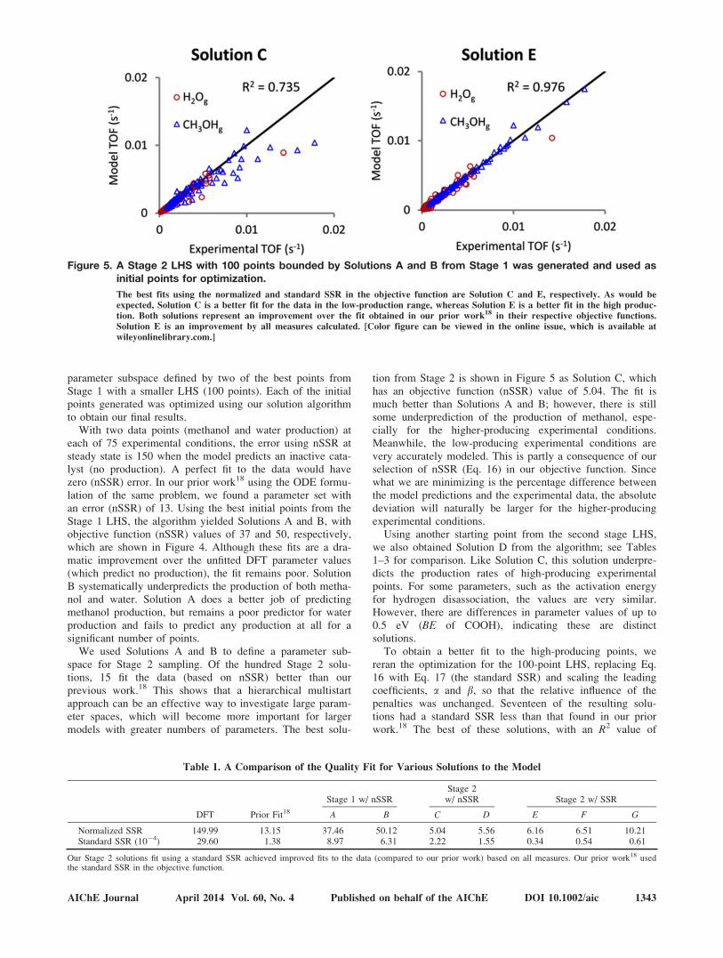
tion from Stage 2 is shown in Figure 5 as Solution C, whichhas an objective function (nSSR) value of 5.04. The fit ismuch better than Solutions A and B; however, there is stillsome underprediction of the production of methanol, espe-cially for the higher-producing experimental conditions.Meanwhile, the low-producing experimental conditions arevery accurately modeled. This is partly a consequence of ourselection of nSSR (Eq. 16) in our objective function. Sincewhat we are minimizing is the percentage difference betweenthe model predictions and the experimental data, the absolutedeviation will naturally be larger for the higher-producingexperimental conditions.

Using another starting point from the second stage LHS,we also obtained Solution D from the algorithm; see Tables1–3 for comparison. Like Solution C, this solution underpre-dicts the production rates of high-producing experimentalpoints. For some parameters, such as the activation energyfor hydrogen disassociation, the values are very similar.However, there are differences in parameter values of up to0.5 eV (BE of COOH), indicating these are distinctsolutions.

To obtain a better fit to the high-producing points, wereran the optimization for the 100-point LHS, replacing Eq.16 with Eq. 17 (the standard SSR) and scaling the leadingcoefficients, a and b, so that the relative influence of thepenalties was unchanged. Seventeen of the resulting solu-tions had a standard SSR less than that found in our priorwork.18 The best of these solutions, with an R2 value of

Figure 5. A Stage 2 LHS with 100 points bounded by Solutions A and B from Stage 1 was generated and used asinitial points for optimization.

The best fits using the normalized and standard SSR in the objective function are Solution C and E, respectively. As would be

expected, Solution C is a better fit for the data in the low-production range, whereas Solution E is a better fit in the high produc-

tion. Both solutions represent an improvement over the fit obtained in our prior work18 in their respective objective functions.

Solution E is an improvement by all measures calculated. [Color figure can be viewed in the online issue, which is available at

wileyonlinelibrary.com.]

Table 1. A Comparison of the Quality Fit for Various Solutions to the Model

DFT Prior Fit18

Stage 1 w/ nSSRStage 2

w/ nSSR Stage 2 w/ SSR

A B C D E F G

Normalized SSR 149.99 13.15 37.46 50.12 5.04 5.56 6.16 6.51 10.21Standard SSR (1024) 29.60 1.38 8.97 6.31 2.22 1.55 0.34 0.54 0.61

Our Stage 2 solutions fit using a standard SSR achieved improved fits to the data (compared to our prior work) based on all measures. Our prior work18 usedthe standard SSR in the objective function.



0.98, (SSR 5 3.4e-5) is shown in Figure 5 as Solution E. (Incomparison, our prior work18 had an R2 value of 0.88 and anSSR of 1.4e-4.) The fit is very good, with nearly all of thedata points lying on or very near the parity line. We alsoinclude Solutions F and G from this set of solutions inTables 1–3, to allow comparisons between their parametervalues.

Table 1 includes the normalized and standard sum ofsquared errors for each solution, allowing us to compare andcontrast the different solutions. Overall our Stage 2 samplingusing the standard SSR provided the best solutions. Theyhave the highest R2 values and the lowest values for SSR.Their nSSR values are lower than those from our priorwork.18 The Stage 2 sampling optimized with nSSR in theobjective function had lower values of nSSR, but the fit ispoor for high-producing experimental points (Figure 5).

Tables 2 and 3 contain the BE and Ea values for selectedfits, respectively. The fits are distinct in their parameter val-ues. Certain parameters are fairly consistent across all solu-tions (such as Ea for HCOOH* 1 H* ! CH3O2* 1 * andBE of CO). Other parameters vary widely from solution tosolution (such as the BE HCO and Ea HCO* 1 H * !

CH2O* 1 *). Because we have identified several solutions ofsimilar quality, with different parameter sets, it is necessaryto consider additional factors to identify the best fit to thedata. These may include considering more than one measureof fit (such as standard and normalized SSR and R2 value),privileging solutions whose parameters most resemble DFT,and examining subsets of the data and evaluating the mod-el’s ability to accurately predict trends in production basedon temperature, pressure, feed composition, reaction orderswith respect to reactants and products, and so forth. Themodel may also be validated by comparing the predictionsof the fitted model to a dataset not used in the fitting. Wewill further investigate these directions in future work.

Conclusions

Reformulating microkinetic models as systems of nonlin-ear equations requires careful scaling and bounding to pro-duce meaningful results. However, it pays off in dramaticimprovements in computational speed. This allows morecomprehensive searches of the parameter space than werepreviously feasible. In the past, the initial values of the

Table 2. BE Values (eV) for DFT, Best Fit from Our Prior Work, and Selected Fits from this Work

DFT Prior Fit18

104-point LHSw/ nSSR

100-point LHSw/ nSSR

100-point LHSw/ SSR

A B C D E F G

CO 20.9 20.8 20.9 21.1 21.0 21.0 21.0 21.3 21.0H2O 20.2 20.2 20.3 20.3 20.2 20.4 20.3 20.5 20.4H 22.4 22.5 22.5 22.4 22.4 22.5 22.5 22.5 22.4CO2 20.1 20.1 20.1 20.3 20.2 20.4 20.3 20.1 20.2OH 22.8 23.2 23.1 23.3 23.1 23.2 23.3 23.0 23.2COOH 21.5 21.8 21.5 21.5 21.5 22.0 21.5 21.5 21.5HCOOH 20.2 20.7 20.9 20.8 20.8 21.2 20.9 21.3 21.1HCO 21.2 21.7 21.7 22.2 22.0 22.0 22.3 21.9 22.1HCO2 22.7 23.3 23.1 23.0 23.1 23.2 23.2 23.3 23.2CH3O2 22.0 22.6 23.1 22.5 23.0 22.9 22.8 23.2 22.9CH2O 20.0 20.5 20.8 20.1 20.6 20.3 20.3 20.8 20.4CH3O 22.5 23.1 23.1 22.5 22.9 22.5 22.8 22.7 22.7CH3OH 20.3 20.5 20.5 20.5 20.5 20.3 20.3 20.4 20.3

There are differences of more than 1 eV between BE values in our present work and DFT predictions (e.g., HCO). There are also differences of more than 0.5eV between solutions from our current work (e.g., CH2O). There are other species for which all solutions have very similar BE values (e.g., H, H2O, andCH3OH). Solutions from Figures 4 and 5 in bold.

Table 3. Ea Values (eV) for DFT, Best Fit from Our Prior Work, and Selected Fits from this Work

DFT Prior Fit18

104-pointLHS w/ nSSR

100-pointLHS w/ nSSR 100-point LHS w/ SSR

A B C D E F G

R1 H2 1 2* ! 2 H* 0.5 0.4 0.5 0.5 0.5 0.5 0.5 0.5 0.5R2 H2O* 1 * ! H* 1 OH* 1.1 0.7 1.0 0.6 0.9 1.1 0.9 1.0 1.0R3 CO* 1 OH* ! COOH* 1 * 0.5 0.5 1.0 0.9 1.0 1.0 0.9 1.0 0.9R4 COOH* 1 * ! CO2* 1 H* 1.0 1.2 1.0 1.0 1.0 0.5 1.0 1.0 1.0R5 CO* 1 H* ! HCO* 1 * 0.9 0.5 1.1 1.1 1.1 1.1 1.1 1.4 1.1R6 CO2* 1 H* ! HCO2* 0.8 0.4 0.6 0.6 0.6 1.1 0.6 0.8 0.7R7 HCO2* 1 H* ! HCOOH* 1 * 0.8 0.9 1.3 0.8 1.0 1.0 1.2 1.1 1.1R8 HCOOH* 1 H* ! CH3O2* 1 * 1.0 1.0 0.9 0.8 1.0 1.1 1.0 1.0 1.0R9 HCO* 1 H* ! CH2O* 1 * 0.4 0.5 0.5 0.6 0.5 0.6 1.0 0.6 0.6R10 CH2O* 1 H* ! CH3O* 1 * 0.2 0.2 0.4 0.1 0.4 0.2 0.3 0.6 0.4R11 CH3O2* 1 * ! CH2O* 1 OH* 0.6 0.4 0.9 0.6 0.8 0.8 0.6 1.0 0.8R12 CH3O* 1 H* ! CH3OH* 1 * 1.1 1.4 1.2 0.6 1.1 0.8 1.1 1.1 0.7

There are differences of more than 0.5 eV between Ea values in our present work and DFT predictions (e.g., R3, R4, R5, and R9). There are also differences ofmore than 0.4 eV between solutions from our current work (e.g., R9, R11, and R12). There are other reactions for which all solutions in our current work havevery similar Ea values (e.g., R1, R2, and R3). Solutions from Figures 4 and 5 in bold.


parameters were adjusted manually based on intuition,knowledge of the system and the gradient at the currentpoint. This approach was very time-consuming and yieldedresults that were heavily dependent upon the skill andknowledge of the user. Moreover, as the process was guidedby prior assumptions about the system, the results were lesslikely to provide novel insights. Our improved approachallowed us to identify multiple fits to the data which are sig-nificantly better than those previously identified. Thisapproach can be extended to reaction networks includingmultiple reaction pathways to identify which are feasible andmost probable. We can further improve our approach byusing more refined, statistically based, objective functions.Greater insight into the reaction on industrially relevant cata-lysts can help us develop better catalysts and better condi-tions for operating existing catalysts. Moreover, thetechniques described herein can be directly extended to theproblem of designing better catalysts, by allowing us tomodel new catalysts in silico much more efficiently than waspreviously possible.

Acknowledgments

This contribution is dedicated to the 90th birthday celebra-tion of R. B. Bird. His legacy of excellence and scientificrigor has inspired generations of Chemical Engineers, includ-ing MM, CTM, LTB, and LCG. The authors acknowledgeDOE-Basic Energy Sciences and 3M for partial financialsupport. LTB acknowledges the Hougen Visiting Professor-ship Fund. The computational work was performed in partusing supercomputing resources from the following institu-tions: EMSL, a National scientific user facility at PacificNorthwest National Laboratory (PNNL); the Center forNanoscale Materials at Argonne National Laboratory (ANL);and the National Energy Research Scientific Computing Cen-ter (NERSC). EMSL is sponsored by the Department ofEnergy’s Office of Biological and Environmental Researchlocated at PNNL. CNM and NERSC are supported by theU.S. Department of Energy, Office of Science, under con-tracts DE-AC02-06CH11357, and DE-AC02-05CH11231,respectively.

Literature Cited

1. Bartholomew CH, Farrauto RJ. Fundamentals of Industrial CatalyticProcesses, 2nd ed. Hoboken, NJ: Wiley, 2006.

2. Greeley J, Norskov JK, Mavrikakis M. Electronic structureand catalysis on metal surfaces. Annu Rev Phys Chem. 2002;53:319–348.

3. Donazzi A, Maestri M, Michael BC, Beretta A, Forzatti P, GroppiG, Tronconi E, Schmidt LD, Vlachos DG. Microkinetic modeling ofspatially resolved autothermal CH4 catalytic partial oxidation experi-ments over Rh-coated foams. J Catal. 2010;275(2):270–279.

4. Dumesic JA. The Microkinetics of Heterogeneous Catalysis. Wash-ington, D.C.: American Chemical Society, 1993.

5. Cortwright R, Dumesic J. Kinetics of heterogeneous catalytic reac-tions: analysis of reaction schemes. Adv Catal. 46;2001:161–264.

6. Gokhale AA, Kandoi S, Greeley JP, Mavrikakis M, Dumesic JA.Molecular-level descriptions of surface chemistry in kinetic modelsusing density functional theory. Chem Eng Sci. 2004;59(22–23):4679–4691.

7. Mhadeshwar AB, Wang H, Vlachos DG. Thermodynamic consis-tency in microkinetic development of surface reaction mechanisms.J Phys Chem B. 2003;107(46):12721–12733.

8. Lynggaard H, Andreasen A, Stegelmann C, Stoltze P. Analysis ofsimple kinetic models in heterogeneous catalysis. Prog Surf Sci.2004;77(3–4):71–137.

9. Ovesen CV, Clausen BS, Schiotz J, Stoltze P, Topsoe H, NorskovJK. Kinetic implications of dynamical changes in catalyst morphol-

ogy during methanol synthesis over Cu/ZnO catalysts. J Catal. 1997;168(2):133–142.

10. Biegler LT. Nonlinear Programming: Concepts, Algorithms, andApplications to Chemical Processes. Philadelphia, PA: Society forIndustrial and Applied Mathematics, 2010.

11. Grossmann IE, Biegler LT. Part II. Future perspective on optimiza-tion. Comput Chem Eng. 2004;28(8):1193–1218.

12. Herder PM, Stikkelman RM. Methanol-based industrial clusterdesign: a study of design options and the design process. Ind EngChem Res. 2004;43(14):3879–3885.

13. Fang K, Li D, Lin M, Xiang M, Wei W, Sun Y. A short review ofheterogeneous catalytic process for mixed alcohols synthesis via syn-gas. Catal Today. 2009;147(2):133–138.

14. Specht M, Staiss F, Bandi A, Weimer T. Comparison of the renew-able transportation fuels, liquid hydrogen and methanol, withgasoline-energetic and economic aspects. Int J Hydrogen Energy.1998;23(5):387–396.

15. Ma J, Sun NN, Zhang XL, Zhao N, Xiao F, Wei W, Sun Y. A shortreview of catalysis for CO2 conversion. Catal Today. 2009;148(3–4):221–231.

16. Olah GA, Goeppert A, Prakash GKS. Chemical recycling off carbondioxide to methanol and dimethyl ether: from greenhouse gas torenewable, environmentally carbon neutral fuels and synthetic hydro-carbons. J Org Chem. 2009;74(2):487–498.

17. Lim HW, Park MJ, Kang SH, Chae HJ, Bae JW, Jun KW. Modelingof the kinetics for methanol synthesis using Cu/ZnO/Al2O3/ZrO2catalyst: influence of carbon dioxide during hydrogenation. Ind EngChem Res. 2009;48(23):10448–10455.

18. Grabow L, Mavrikakis M. On the mechanism of methanol synthesison Cu through CO and CO2 hydrogenation. ACS Catal. 2011;1:365–384.

19. Rostamikia G, Mendoza AJ, Hickner MA, Janik MJ. First-principlesbased microkinetic modeling of borohydride oxidation on a Au(111)electrode. J Power Sources. 2011;196(22):9228–9237.

20. Cao XM, Burch R, Hardacre C, Hu P. Reaction mechanisms ofcrotonaldehyde hydrogenation on Pt(111): density functionaltheory and microkinetic modeling. J Phys Chem C. 2011;115(40):19819–19827.

21. Madon RJ, Braden D, Kandoi S, Nagel P, Mavrikakis M, DumesicJA. Microkinetic analysis and mechanism of the water gas shift reac-tion over copper catalysts. J Catal. 2011;281(1):1–11.

22. Thybaut JW, Sun JJ, Olivier L, Van Veen AC, Mirodatos C, MarinGB. Catalyst design based on microkinetic models: oxidative cou-pling of methane. Catal Today. 2011;159(1):29–36.

23. Liu K, Wang A, Zhang W, Wang J, Huang Y, Wang X, Shen J,Zhang T. Microkinetic study of CO oxidation and PROX on Ir-FeCatalyst. Ind Eng Chem Res. 2011;50(2):758–766.

24. Bligaard T, Norskov JK, Dahl S, Matthiesen J, Christensen CH,Sehested J. The Bronsted-Evans-Polanyi relation and the volcanocurve in heterogeneous catalysis. J Catal. 2004;224(1):206–217.

25. Hansgen DA, Vlachos DG, Chen JGG. Using first principles to pre-dict bimetallic catalysts for the ammonia decomposition reaction.Nat Chem. 2010;2(6):484–489.

26. Nocedal J, Wright SJ. Numerical Optimization, 2nd ed. New York:Springer; 2006.

27. Alexe M, Sandu A. Forward and adjoint sensitivity analysis withcontinuous explicit Runge-Kutta schemes. Appl Math Comput. 2009;208(2):328–346.

28. Cao Y, Li ST, Petzold L. Adjoint sensitivity analysis for differential-algebraic equations: algorithms and software. 15th Toyota Confer-ence on Scientific and Engineering Computations for the 21st Cen-tury. Mikkabi, Japan, October 28–31, 2001.

29. Cao Y, Li ST, Petzold L, Serban R. Adjoint sensitivity analysis ofdifferential-algebraic equations: the adjoint DAE system and itsnumerical solution. SIAM J Sci Comput. 2002;24(3):1076–1089.

30. Sandu A, Daescu DN, Carmichael GR. Direct and adjoint sensitivityanalysis of chemical kinetic systems with KPP: part I - theory andsoftware tools. Atmos Environ. 2003;37(36):5083–5096.

31. Tanartkit P, Biegler LT. Reformulating ill-conditioned differential-algebraic equation optimization problems. Ind Eng Chem Res. 1996;35(6):1853–1865.

32. Vassiliadis VS, Floudas CA. The modified barrier function approachfor large-scale optimization. Comput Chem Eng. 1997;21(8):855–874.

33. Wright MH. Ill-conditioning and computational error in interiormethods for nonlinear programming. SIAM J Optim. 1998;9(1):84–111.


34. Graaf GH, Stamhuis EJ, Beenackers A. Kinetics of low-pressuremethanol synthesis. Chem Eng Sci. 1988;43(12):3185–3195.

35. Rubin DB, Gelman A, Carlin JB, Stern H. Bayesian Data Analysis,2nd ed. Boca Raton: Chapman & Hall/CRC, 2003.

36. Drud A. Conopt - a grg code for large sparse dynamic nonlinearoptimization problems. Math Program. 1985;31(2):153–191.

37. Drud A, CONOPT. ARKI Consulting and Development A/S, Bags-vaerd, Denmark, GAMS Solver Manual. http://www.gams.com/solv-ers/index.htm (Last accessed: Dec 2013).

38. Brooke A, Kendrick D, Meeraus A. (1988). GAMS: A User’s Guide.The Scientific Press, San Francisco, CA.

39. Ugray Z, Lasdon L, Plummer J, Glover F, Kelly J, Marti R. Scattersearch and local NLP solvers: a multistart framework for global opti-mization. Inform J Comput. 2007;19(3):328–340.

40. Ugray Z, Lasdon L, Plummer JC, Bussieck M. Dynamic filters andrandomized drivers for the multi-start global optimization algorithmMSNLP. Optim Methods Softw. 2009;24(4–5):635–656.

41. Stein M. Large sample properties of simulations using latin hyper-cube sampling. Technometrics. 1987;29(2):143–151.

Manuscript received Sept. 18, 2013, and revision received Nov. 18, 2013.


http://www.gams.com/solvers/index.htm

http://www.gams.com/solvers/index.htm

advanced solution methods for microkinetic models of catalytic reactions: a methanol synthesis case...

Documents