advanced reactors-intermediate heat exchanger (ihx ... reports/fy 2012/12-3363 neup... · advanced...
TRANSCRIPT

Advanced Reactors-Intermediate Heat Exchanger (IHX) Coupling:
Theoretical Modeling and Experimental Validation
Reactor Concepts Research Development and Demonstration (RDRD&D)
Vivek Utgikar University of Idaho
In collabora2on with:
The Ohio State University
Carl Sink, Federal POC Michael McKellar, Technical POC
Project No. 12-3363

Final Report
Project Title: Advanced Reactors-Intermediate Heat Exchanger (IHX) Coupling:
Theoretical Modeling and Experimental Validation
Date of Report: December 29, 2016
Milestone Level: 2
Recipient: University of Idaho
Office of Sponsored Programs
P.O. Box 443020
Moscow ID 83844
Award Number: 128504
Project Number: 12-3363
Project Period: September 10, 2012 – September 30, 2016
Principal: Utgikar, Vivek
Investigator 208-885-6970
Collaborators: Sun, Xiaodong (The Ohio State University)
614-247-7646
Christensen, Richard N. (The Ohio State University/University of Idaho)
208-533-8102
Sabharwall, Piyush (Idaho National Laboratory)
208-526-6494
TPOC Michael McKellar
Federal Manager Carl Sink
Workscope NGNP-2
i
Executive Summary
Goals, Objectives, and Approach
The overall goal of the research project was to model the behavior of the advanced reactor-
intermediate heat exchange system and to develop advanced control techniques for off-normal conditions.
The specific objectives defined for the project were:
1. To develop the steady-state thermal hydraulic design of the intermediate heat exchanger (IHX);
2. To develop mathematical models to describe the advanced nuclear reactor-IHX-chemical
process/power generation coupling during normal and off-normal operations, and to simulate models
using multiphysics software;
3. To develop control strategies using genetic algorithm or neural network techniques and couple these
techniques with the multiphysics software;
4. To validate the models experimentally
The project objectives were accomplished by defining and executing four different tasks
corresponding to these specific objectives. The first task involved selection of IHX candidates and
developing steady state designs for those. The second task involved modeling of the transient and off-
normal operation of the reactor-IHX system. The subsequent task dealt with the development of control
strategies and involved algorithm development and simulation. The last task involved experimental
validation of the thermal hydraulic performances of the two prototype heat exchangers designed and
fabricated for the project at steady state and transient conditions to simulate the coupling of the reactor-
IHX-process plant system. The experimental work utilized the two test facilities at The Ohio State
University (OSU) including one existing High-Temperature Helium Test Facility (HTHF) and the newly
developed high-temperature molten salt facility.
Accomplishments and Outcomes
The summary of these activities conducted and the resulting outcomes is as follows:
Steady state designs for four different candidate compact heat exchanger designs – Wavy-
Channel Printed Circuit Heat Exchanger (PCHE), Offset Strip-Fin Heat Exchanger (OSFHE),
Helical Coil Heat Exchanger (HCHE), and Twisted Tube Heat Exchanger (TTHE) – were
completed for various combinations of primary and secondary heat transfer media that included
helium and fluoride salts.
ii
Mathematical models for describing the transient behavior of the advanced reactor-IHX-process
application system were developed. Model simulations were conducted through development of
MATLAB programs, as well as by using commercially available process simulation programs
PRO/II and Dynsim.
The system was analyzed with respect to possible disturbances and their impacts on the system.
Three control blocks – Reactor, Intermediate Heat Exchanger (IHX), and Secondary Heat
Exchanger (SHX) – were defined. Controlled variables, manipulated variables and load variables
(disturbances) were identified for each block. Transfer functions relating the controlled variables
to the manipulated and load variables were developed for the SHX and IHX blocks. Stability
analysis and estimation of controller parameters was conducted on the basis of the transfer
functions.
Dynamics and control of the system were simulated for various scenarios using user developed
MATLAB codes. It was found that the disturbances in the primary loop had an overall greater
impact on the system than the disturbances in other loops. It may be best to have a control
strategy in which the manipulated variables depend on where the disturbance occurs. In addition,
switching of the manipulated variable after a certain pre-set limit (+20% change in the
manipulated variable) was reached for that variable was investigated. This limit is reached for
large temperature disturbances in the system, which triggered a switching of the manipulated
variables. Using this approach, the system was able to control the variables at their set points.
The behavior of the system under a comprehensive control scheme, where the nuclear reactor
operation is also controlled, was also simulated. The reactor model included the point kinetic
equations with 3 groups of delayed neutrons, which achieved the best balance between the
computational load and accuracy. Various control options were investigated that included
manipulating flow rates, or reactor power or a combination thereof. Each option was successful in
resetting the controlled variables to their set points.
A comprehensive model was developed to obtain the dynamics of the helium Brayton Cycle PCS
in response to any system disturbances. Temperature transients of various streams in response to
different disturbance stimuli were obtained indicating the utility of this approach.
Prototype wavy-channel (zigzag) printed circuit heat exchanger (PCHE) and helically-coiled
twisted tube heat exchangers were designed and fabricated for experimental testing. Experiments
were also conducted with an available straight channel PCHE.
The PCHE testing was conducted in the HTHF. Experimental data were obtained by introducing
disturbances in the laboratory and monitoring the response. Transient numerical models
iii
developed for the PCHE were run and validated by comparison with the dynamic test data. The
data indicate that the transient model can accurately predict the behavior of the system.
Thermal-hydraulic performance testing of the helically-coiled fluted tube heat exchanger was
conducted under water to water conditions. Experimental data were analyzed for the pressure
drop, thermal duty, heat loss, and heat exchanger effectiveness aspects. The heat exchanger
effectiveness values obtained from the experiments compared well with those obtained from
theoretical calculations.
Refereed Journal Publications
A) Published
1. Bartel N, Chen M, Utgikar VP, Sun X, Kim I-H, Christensen R, Sabharwall P. 2015. Comparison
of compact heat exchangers for application as the intermediate heat exchanger for advanced
nuclear reactors. Annals of Nuclear Energy, 81: 143-149.
2. Chen M, Kim I, Sun X, Christensen RN, Utgikar V, Sabharwall P. 2015. Transient analysis of an
FHR coupled to a helium Brayton cycle. Progress in Nuclear Energy, 83: 283-293.
3. Skavdahl I, Utgikar V, Sabharwall P, Chen M, Sun X, Christensen R. 2016. Modeling and
Simulation of Control System Response to Temperature Disturbances in a Coupled Heat
Exchangers-AHTR System. Nuclear Engineering and Design, 300: 161-172, DOI
10.1016/j.nucengdes.1016.01.010.
4. Skavdahl I, Utgikar V, Christensen R, Chen M, Sun X, Sabharwall P. 2016. Control of Advanced
Reactor-Coupled Heat Exchangers System: Incorporation of Reactor Dynamics in System
Response to Load Disturbances. Nuclear Engineering and Technology, 48: 1349-1359, DOI:
10.1016/j.net.2016.05.001.
5. Chen M, Sun X, Christensen R, Shi S, Skavdahl I, Utgikar V, Sabharwall P. 2016. Experimental
and Numerical Study of a Printed Circuit Heat Exchanger. Annals of Nuclear Energy, 97: 221-
231, DOI 10.1016/j.anucene.2016.07.010.
6. Chen M, Sun X, Christensen R, Skavdahl I, Utgikar V, Sabharwall P. 2016. Pressure Drop and
Heat Transfer Characteristics of a High-temperature Printed Circuit Heat Exchanger. Applied
Thermal Engineering, 108: 1409-1417, DOI 10.1016/j.applthermaleng.2016.07.149.
B) In Progress
1. Chen M, Sun X, Christensen RN, Skavdahl I, Utgikar V, and Sabharwall P. “Transient Analysis
of a High-Temperature Printed Circuit Heat Exchanger: Numerical Modeling and Experimental
Investigation,” submission to Nuclear Engineering and Design. (In revision)
iv
2. Skavdahl I, Utgikar V, Torres C, Chen M, Sun X, Christensen R, Sabharwall P. “Determination
of the Dynamic Behavior of the Advanced Reactor-Heat Exchanger System using Process
Simulation Softwares,” submission to Journal of Thermal Science and Engineering Applications
(In review).
Conference Papers and Presentations
1. “Thermal-Hydraulic Design of Wavy-Channel Printed Circuit Heat Exchangers,” N Bartel, V
Utgikar, M Chen, X Sun, I-H Kim, R Christensen, P Sabharwall, 2013 ANS Annual Meeting,
June 2013, Atlanta, Georgia.
2. “Design of Printed Circuit Heat Exchangers for Very High Temperature Reactors,” M Chen, X
Sun, I-H Kim, R Christensen, N Bartel, V Utgikar, P Sabharwall, 2013 ANS Annual Meeting,
June 2013, Atlanta, Georgia.
3. “Dynamic Response Analysis of a Scaled-Down Offset Strip-Fin Intermediate Heat Exchanger,”
M Chen, I-H Kim, X Sun, RN Christensen, N Bartel, V Utgikar, and P. Sabharwall, 2013 ANS
Winter Meeting, November 2013, Washington, DC.
4. “Transient Model of Wavy-Channel Printed Circuit Heat Exchangers,” N Bartel, V Utgikar, P
Sabharwall, M Chen, X Sun, I-H Kim, RN Christensen, 2013 ANS Winter Meeting, November
2013, Washington, DC.
5. “Transient Analysis of Advanced High Temperature Reactors Using Process Simulation
Software,” I Skavdahl, V Utgikar, P Sabharwall, M Chen, X Sun, I-H Kim, RN Christensen, 2014
ANS Winter Meeting, November 2014, Anaheim, California.
6. “Preliminary Design of a Helical Coil Heat Exchanger for a Fluoride Salt-Cooled High-
Temperature Test Reactor,” M Chen, I Kim, X Sun, RN Christensen, I Skavdahl, V Utgikar, and
P Sabharwall, 2014 ANS Winter Meeting, November 2014, Anaheim, California.
7. “Control Strategy Development of Advanced High Temperature Reactor System,” I Skavdahl, V
Utgikar, P Sabharwall, M Chen, X Sun, R Christensen, 2015 Annual Meeting of the ANS, June
2015, San Antonio, Texas.
8. “Simulation of Advanced High Temperature Reactor Control System using MATLAB,” I
Skavdahl, V Utgikar, P Sabharwall, M Chen, X Sun, R Christensen, 2015 Winter meeting of the
American Nuclear Society (ANS), November 2015, Washington, DC.
9. “Development of a Thermal-Hydraulic Analysis Code for an FHR,” M Chen, X Sun, RN
Christensen, S Shi, I Skavdahl, V Utgikar, P Sabharwall, 11th International Topical Meeting on
Nuclear Reactor Thermal Hydraulics, Operation and Safety (NUTHOS-11), October 2016,
Gyeongju, South Korea.
v
10. “Experimental and Numerical Study of Heat Transfer and Pressure Drop in a High-Temperature
Printed Circuit Heat Exchanger,” M Chen, S Shi, X Sun, RN Christensen, I Skavdahl, V Utgikar,
P Sabharwall, 8th International Topical Meeting on High Temperature Reactor Technology 2016
(HTR2016), November 2016, Las Vegas, NV.
11. “Helium Brayton Cycle Design for Advanced High Temperature Reactor System,” I Skavdahl, V
Utgikar, R Christensen, P Sabharwall, M Chen, X Sun, 2016 ANS Winter Meeting, November
2016, Las Vegas, NV.
Mentoring of Students
1. Isaac Skavdahl, M.S. (Major: Chemical Engineering), University of Idaho, Spring 2016.
Thesis: Analysis of transients and control of advanced high temperature reactor-coupled heat
exchangers system.
2. Minghui Chen, M.S. (Major: Nuclear Engineering), The Ohio State University, Summer 2015.
Thesis: Design, fabrication, testing, and modeling of a high-temperature printed circuit heat
exchanger.
3. Minghui Chen, Ph.D. (Major: Nuclear Engineering), The Ohio State University, In Progess.
Dissertation: Performance testing and Dynamic modeling of high-temperature heat exchangers
for an FHR.
4. Cesar Torres, B.S. (Major: Chemical Engineering), University of Idaho, Fall 2015.
Undergraduate research assistant.
5. Michael Cron, B.S. (Major: Chemical Engineering), Spring 2014.
Undergraduate research assistant.
6. Nathan Bartel, M.S. (Major: Nuclear Engineering), University of Idaho.
vi
Table of Contents
Executive Summary ....................................................................................................................................... i
1. Introduction ........................................................................................................................................... 1
1.1 Goals and Objectives ...................................................................................................................... 2
1.2 Research Approach and Methods ................................................................................................... 2
2. Steady State Thermal Hydraulic Design of Heat Exchangers............................................................... 3
2.1 Printed Circuit Heat Exchanger (PCHE) ........................................................................................ 4
2.2 Offset Strip-Fin PCHE .................................................................................................................. 11
2.3 Helical Coil Heat Exchanger ........................................................................................................ 17
2.4 Twisted Tube Heat Exchanger (TTHE) ........................................................................................ 23
2.5 Summary ....................................................................................................................................... 27
3. Modeling of Advanced Reactor-IHX System Transients ................................................................... 27
3.1 System Analysis with Simulation Software .................................................................................. 28
3.1.1 PRO/II Model ...................................................................................................................... 28
3.1.2 Dynsim Flowsheet and Modeling........................................................................................ 31
3.1.3 Simulation of System Behavior for Flow Rate Disturbances .............................................. 33
3.1.4 Incorporation of Nuclear Reactor in Dynsim ...................................................................... 42
3.1.5 Transients after Temperature Disturbances ......................................................................... 45
3.1.6 Process Simulation Results Summary ................................................................................. 48
3.2. Mathematical Modeling using User-Developed Programs .......................................................... 48
3.2.1 Steady-state simulations ...................................................................................................... 49
3.2.2 Transient simulations for Straight-Channel PCHE ............................................................. 50
3.2.3 Transient simulations for Zig-Zag Channel PCHE ............................................................. 54
3.3 Verification ................................................................................................................................... 59
3.4 Summary ....................................................................................................................................... 59
4. Control System Design and Response .................................................................................................... 60
4.1 Advanced Reactor-Heat Exchanger System ................................................................................. 60
4.2 Helium Brayton Cycle Power Conversion System (PCS) ............................................................ 61
4.3 Control System Architecture ........................................................................................................ 61
4.3.1 Control Methodology .......................................................................................................... 62
4.3.2 Block Diagrams ................................................................................................................... 63
4.3.3 Controller Development ...................................................................................................... 65
4.3.4 System Disturbances ........................................................................................................... 66
vii
4.4 System Models and Simulation Technique................................................................................... 67
4.4.1 Governing Equations for Heat Exchangers ......................................................................... 67
4.4.2 Governing Equations for Reactor ........................................................................................ 68
4.4.3 Numerical Solution Technique ............................................................................................ 69
4.5 Results and Discussion ................................................................................................................. 70
4.5.1 Controlled response of coupled heat exchangers system .................................................... 70
4.5.2 Controlled response of coupled heat exchangers-reactor system ........................................ 81
4.5.3 Modeling and simulation of helium Brayton Cycle PCS .................................................... 94
4.6 Summary ..................................................................................................................................... 104
5. Experimental Validation ................................................................................................................... 106
5.1 Description of Facilities .............................................................................................................. 106
5.1.1 High-Temperature Helium Facility (HTHF) ..................................................................... 106
5.1.2 High-Temperature Molten Salt Facility ............................................................................ 107
5.2 Design and Fabrication of Heat Exchangers ............................................................................... 108
5.2.1 Wavy Channel PCHE ........................................................................................................ 108
5.2.2 Helically Coiled Twisted Tube Heat Exchanger ........................................................... 112
5.2.3 Straight-Channel PCHE .................................................................................................... 117
5.3 Experimental Results .................................................................................................................. 118
5.3.1 Wavy-Channel PCHE ....................................................................................................... 118
5.3.2 Straight Channel PCHE ..................................................................................................... 123
5.3.3 Helically-Coiled Heat Exchanger ...................................................................................... 125
5.4 Summary ..................................................................................................................................... 129
6. Conclusions ....................................................................................................................................... 130
References ................................................................................................................................................. 131
Quad Chart ................................................................................................................................................ 134
1
REPORT NARRATIVE
1. Introduction
Advanced reactors (such as the high temperature gas-cooled reactor – HTGR, or advanced high
temperature reactor – AHTR) from the Gen IV program are required to deliver electricity and process
heat with high efficiency. The electric power production may be through a high-pressure steam generator
(Rankine cycle) or a direct- or indirect-cycle gas turbine (Brayton cycle). The process heat applications
may include co-generation, coal-to-liquids conversion, and synthesis of chemical feedstocks. The process
heat applications of these advanced reactors are critically dependent upon an effective intermediate heat
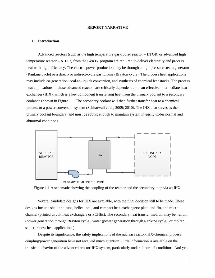
exchanger (IHX), which is a key component transferring heat from the primary coolant to a secondary
coolant as shown in Figure 1.1. The secondary coolant will then further transfer heat to a chemical
process or a power conversion system (Sabharwall et al., 2009; 2010). The IHX also serves as the
primary coolant boundary, and must be robust enough to maintain system integrity under normal and
abnormal conditions.
PRIMARY PUMP/ CIRCULATOR
Figure 1.1 A schematic showing the coupling of the reactor and the secondary loop via an IHX.
Several candidate designs for IHX are available, with the final decision still to be made. These
designs include shell-and-tube, helical coil, and compact heat exchangers: plate-and-fin, and micro-
channel (printed circuit heat exchangers or PCHEs). The secondary heat transfer medium may be helium
(power generation through Brayton cycle), water (power generation through Rankine cycle), or molten
salts (process heat applications).
Despite its significance, the safety implications of the nuclear reactor-IHX-chemical process
coupling/power generation have not received much attention. Little information is available on the
transient behavior of the advanced reactor-IHX system, particularly under abnormal conditions. And yet,
2
this information is critical for the overall safety assessment of the reactor system and therefore for
regulatory design certification review. The normal and off-normal behavior of these reactors differs from
those of conventional light water reactors. The complexity of the system requires the development of
advanced techniques to ensure proper control of the system. This research was conducted to fulfill this
need through the development and application of these advanced techniques to the advanced reactor-IHX
system. The theoretical results were validated through experiments at The Ohio State University.
1.1 Goals and Objectives
The overall goal of the proposed research was to model the behavior of the Advanced Reactor-
IHX-Chemical Process/Power Generation system and develop advanced control techniques for off-normal
conditions. The specific objectives defined for the project were:
1. To develop the steady-state thermal hydraulic design of the intermediate heat exchanger (IHX);
2. To develop mathematical models to describe the advanced nuclear reactor-IHX-chemical
process/power generation coupling during normal and off-normal operations, and to simulate
models using multiphysics software;
3. To develop control strategies using genetic algorithm or neural network techniques and couple
these techniques with the multiphysics software;
4. To validate the models experimentally.
1.2 Research Approach and Methods
The above objectives were accomplished through the execution of the tasks described below:
Task 1: Steady-State Thermal Hydraulic Design of IHX
Candidate heat exchangers types were identified for the IHX application for different combinations of
Primary and secondary coolants and the thermal hydraulic designs developed for the IHXs operating
under various steady-state conditions. Heat exchangers were specified with respect to the design
requirements of output power, inlet and outlet temperatures and mass flow rates of the streams.
Task 2: Modeling of the IHX under Transient and Off-Normal Conditions
The second task involved modeling the behavior of the reactor-IHX system under transient and off-
normal conditions. The transient conditions involved changes in the reactor power output as well as
demand changes from the secondary side (power generation and process applications) due to variations in
flow rates and fluid temperatures.
Task 3: Devising Control Strategy
The complexity of the system requires advanced control techniques to ensure operational safety. Detailed
analysis of the system was conducted to identify the system disturbances (load variables), controlled

3
variables, and manipulated variables. Mathematical models were developed to describe the relationships
(transfer functions) between the various variables, and controllers specified for the system. The control
system response was simulated for various flow and temperature disturbances.
Task 4: Experimental Validation
Prototype IHXs were designed and fabricated for the experimental validation of the system models.
Experiments were conducted using the two test facilities – the high-temperature helium test facility
(HTHF) and the high-temperature molten salt facility at The Ohio State University – to examine the
thermal performance of these IHXs at steady state and transient conditions and to simulate the coupling of
the reactor-IHX-process system.
The activities conducted and results obtained through the research are described in the following
sections, with each section presenting details corresponding to each of the four tasks.
2. Steady State Thermal Hydraulic Design of Heat Exchangers
A literature search of the candidate IHXs was the first step to understanding their applicability to the
nuclear reactor-IHX-chemical process/power generation plant. The literature search helped identify the
printed circuit heat exchanger (PCHE) and offset strip-fin PCHE as the primary candidates. Helical coil
heat exchanger and the twisted tube heat exchanger were the other two candidates identified as of interest.
Operational Parameters
The operational parameters for the heat exchanger designs were modified from the NGNP reference
VHTR system from the Gen-IV Program (Oh and Kim, 2008). The Reactor Outlet Temperature (ROT)
has been decreased from 900 °C to 800 °C due to material concerns and the mass flow rate [kg/s] was
balanced. These operating conditions are shown in Table 2.1 for the Helium/Helium primary and
secondary loop fluid combination.
4
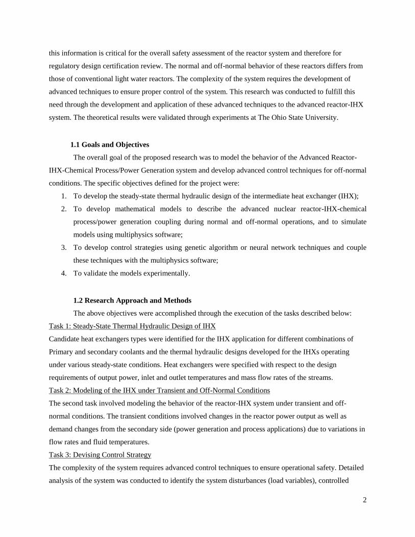
Table 2.1. Operating Conditions for the 600 MWth Design
Parameters
Hot Channel
In Out
Cold Channel
In Out
Fluid Helium Helium T [°C] 800 543 520 776
P [MPa] 7 6.95 7.97 7.92
�̇� [kg/s] 450 450 450 450
𝜌 [kg/m3] 3.117 4.059 4.78 3.603
𝑐𝑝 [kJ/kg-K] 5.19 5.19 5.19 5.19
𝑘 [W/m-K] 0.3822 0.3164 0.3106 0.3767
𝜇 [kg/m-s] 4.859e-05 4.008e-05 3.929e-05 4.783e-05
Prandtl Number 0.66 0.66 0.66 0.66
The different heat exchangers and their thermal hydraulic designs are described below:
2.1 Printed Circuit Heat Exchanger (PCHE)
A PCHE is a type of compact heat exchanger where the coolant flow channels are photo-chemically
etched on one side of thin plates. The fluid passages are approximately semicircular in cross-section.
These plates are then formed into a heat exchanger core through a diffusion bonding process that includes
a thermal soaking period to allow grain growth. This diffusion bonding process enables an interface-free
join between the plates and gives the base material strength and a very high pressure containment
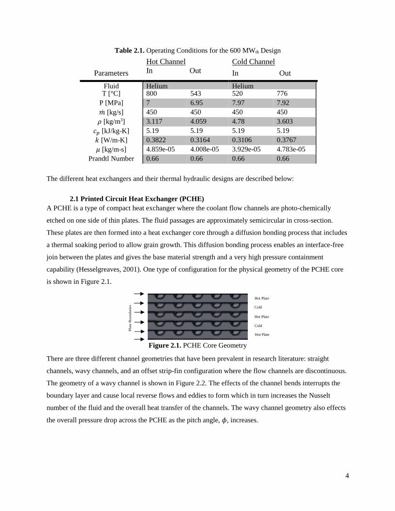
capability (Hesselgreaves, 2001). One type of configuration for the physical geometry of the PCHE core
is shown in Figure 2.1.
Figure 2.1. PCHE Core Geometry
There are three different channel geometries that have been prevalent in research literature: straight
channels, wavy channels, and an offset strip-fin configuration where the flow channels are discontinuous.
The geometry of a wavy channel is shown in Figure 2.2. The effects of the channel bends interrupts the
boundary layer and cause local reverse flows and eddies to form which in turn increases the Nusselt
number of the fluid and the overall heat transfer of the channels. The wavy channel geometry also effects
the overall pressure drop across the PCHE as the pitch angle, 𝜙, increases.
Pla
te B
oundar
ies
Hot Plate
Cold
Plate
Hot Plate
Cold
Plate Hot Plate

5
Figure 2.2. Wavy Channel Geometry (Kim and No, 2012)
The full-scale thermal hydraulic design of the helium/helium wavy channel and offset strip-fin PCHE is
described below. The following assumptions were made for the design: the heat exchanger operates at
steady state, flow distribution in each channel is uniform, the hot and cold plates have equivalent
geometry, the flow passages are approximately semicircular, and heat loss from the PCHE surface is
neglected.
Wavy Channel PCHE:
The flow regime for a semicircular duct can be defined as follows: the laminar region Re 2300 , the
transitional region 2300 Re 10, 000 , and the turbulent region Re 10, 000 .
Laminar Region – Wavy Channel PCHE
The laminar region of semicircular channels in PCHEs has been characterized by Hesselgreaves as
occurring below a Reynolds number of 2300. According to research done by Mylavarapu (2011) the
transition regime occurs at a value much lower than 2300, approximately 1700. The wavy channels
provide constant boundary layer interruption; this makes it very hard to identify where the flow regime
becomes transitional because it is believed that boundary layer effect is much greater than the transitional
flow effect. For the sake of brevity, we will assume that the corresponding critical Reynolds number
identified by Mylavarapu is acceptable for design calculations.
Laminar Flow - Overall Pressure Drop Characteristics:
The Fanning friction factor is used to find the overall pressure drop across the PCHE. The straight
channel Fanning friction factor correlation suggested by Hesselgreaves (2001) for the laminar region is
given by,
Re 15.78 Re 2300f (2.1)
Kim and No (2012) proposed a new correlation modifying Equation 2.1 by using fitting constants for
wavy channel geometries. The fitting constants are dependent on channel pitch angle, ϕ, and single pitch
length. The modified correlation is,
6
Re 15.78 Re Re 2300bf a (2.2)
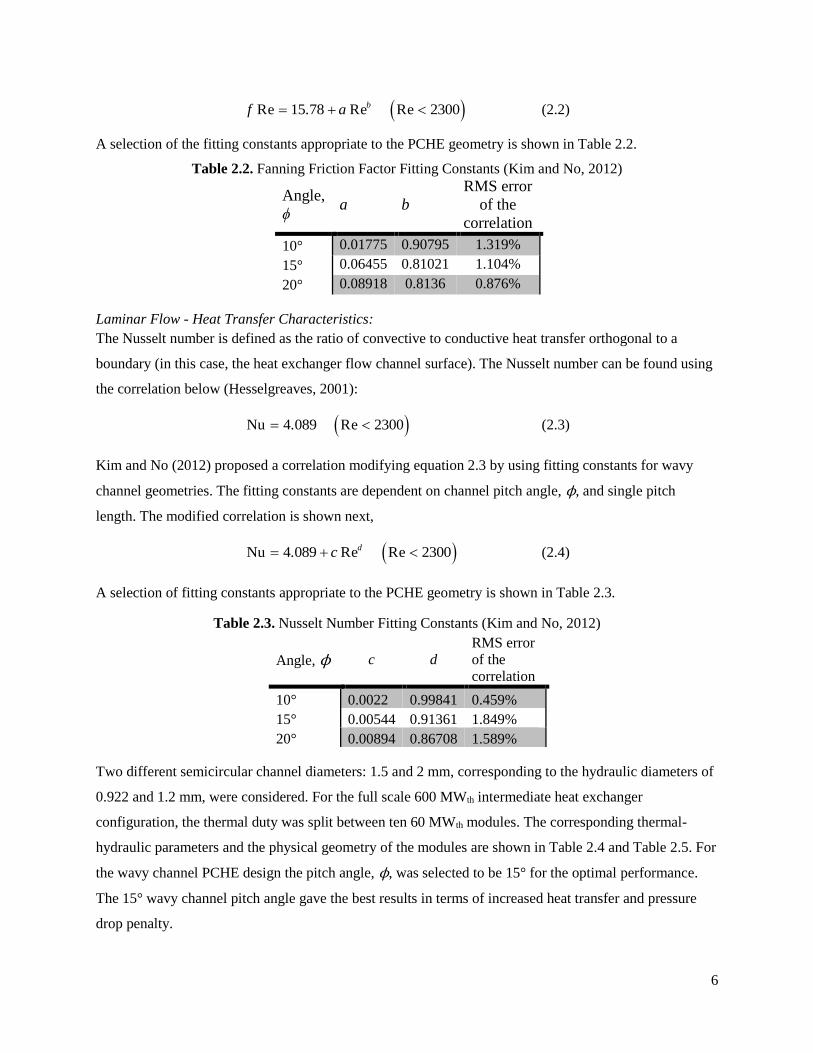
A selection of the fitting constants appropriate to the PCHE geometry is shown in Table 2.2.
Table 2.2. Fanning Friction Factor Fitting Constants (Kim and No, 2012)
Angle,
ϕ a b
RMS error
of the
correlation
10° 0.01775 0.90795 1.319%
15° 0.06455 0.81021 1.104%
20° 0.08918 0.8136 0.876%
Laminar Flow - Heat Transfer Characteristics:
The Nusselt number is defined as the ratio of convective to conductive heat transfer orthogonal to a
boundary (in this case, the heat exchanger flow channel surface). The Nusselt number can be found using
the correlation below (Hesselgreaves, 2001):
Nu 4.089 Re 2300 (2.3)
Kim and No (2012) proposed a correlation modifying equation 2.3 by using fitting constants for wavy
channel geometries. The fitting constants are dependent on channel pitch angle, ϕ, and single pitch
length. The modified correlation is shown next,
Nu 4.089 Re Re 2300dc (2.4)
A selection of fitting constants appropriate to the PCHE geometry is shown in Table 2.3.
Table 2.3. Nusselt Number Fitting Constants (Kim and No, 2012)
Angle, ϕ c d
RMS error
of the
correlation
10° 0.0022 0.99841 0.459%
15° 0.00544 0.91361 1.849%
20° 0.00894 0.86708 1.589%
Two different semicircular channel diameters: 1.5 and 2 mm, corresponding to the hydraulic diameters of
0.922 and 1.2 mm, were considered. For the full scale 600 MWth intermediate heat exchanger
configuration, the thermal duty was split between ten 60 MWth modules. The corresponding thermal-
hydraulic parameters and the physical geometry of the modules are shown in Table 2.4 and Table 2.5. For
the wavy channel PCHE design the pitch angle, ϕ, was selected to be 15° for the optimal performance.
The 15° wavy channel pitch angle gave the best results in terms of increased heat transfer and pressure
drop penalty.
7
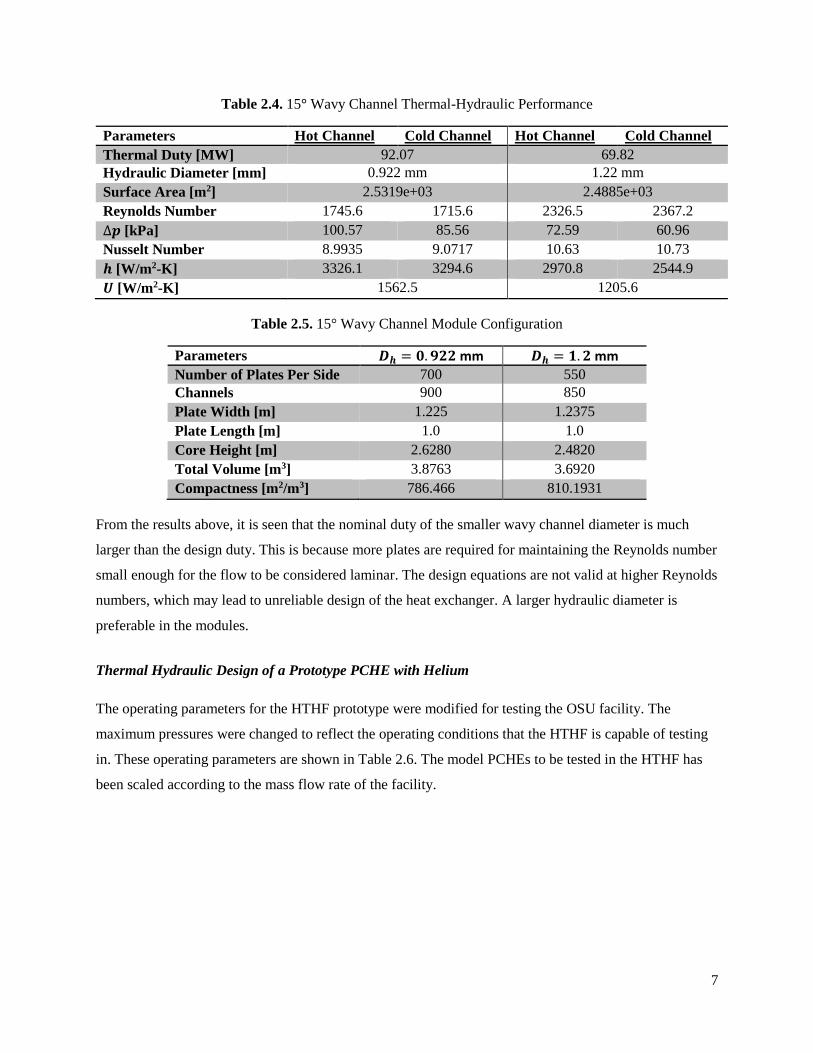
Table 2.4. 15° Wavy Channel Thermal-Hydraulic Performance
Parameters Hot Channel Cold Channel Hot Channel Cold Channel
Thermal Duty [MW] 92.07 69.82
Hydraulic Diameter [mm] 0.922 mm 1.22 mm
Surface Area [m2] 2.5319e+03 2.4885e+03
Reynolds Number 1745.6 1715.6 2326.5 2367.2
∆𝒑 [kPa] 100.57 85.56 72.59 60.96
Nusselt Number 8.9935 9.0717 10.63 10.73
𝒉 [W/m2-K] 3326.1 3294.6 2970.8 2544.9
𝑼 [W/m2-K] 1562.5 1205.6
Table 2.5. 15° Wavy Channel Module Configuration
Parameters 𝑫𝒉 = 𝟎. 𝟗𝟐𝟐 mm 𝑫𝒉 = 𝟏. 𝟐 mm
Number of Plates Per Side 700 550
Channels 900 850
Plate Width [m] 1.225 1.2375
Plate Length [m] 1.0 1.0
Core Height [m] 2.6280 2.4820
Total Volume [m3] 3.8763 3.6920
Compactness [m2/m3] 786.466 810.1931
From the results above, it is seen that the nominal duty of the smaller wavy channel diameter is much
larger than the design duty. This is because more plates are required for maintaining the Reynolds number
small enough for the flow to be considered laminar. The design equations are not valid at higher Reynolds
numbers, which may lead to unreliable design of the heat exchanger. A larger hydraulic diameter is
preferable in the modules.
Thermal Hydraulic Design of a Prototype PCHE with Helium
The operating parameters for the HTHF prototype were modified for testing the OSU facility. The
maximum pressures were changed to reflect the operating conditions that the HTHF is capable of testing
in. These operating parameters are shown in Table 2.6. The model PCHEs to be tested in the HTHF has
been scaled according to the mass flow rate of the facility.
8
Table 2.6. Operating Conditions for the 16 kW Design
Parameters
Hot Channel
In Out
Cold Channel
In Out
Fluid Helium Helium T [°C] 800 543 520 776
P [MPa] 3 2.95 2 1.95
�̇� [kg/s] 0-49 0-49
𝜌 [kg/m3] 3.117 4.059 4.78 3.603
𝑐𝑝 [kJ/kg-K] 5.19 5.19 5.19 5.19
𝑘 [W/m-K] 0.3822 0.3164 0.3106 0.3767
𝜇 [kg/m-s] 4.859e-05 4.008e-05 3.929e-05 4.783e-05
Prandtl Number 0.66 0.66 0.66 0.66
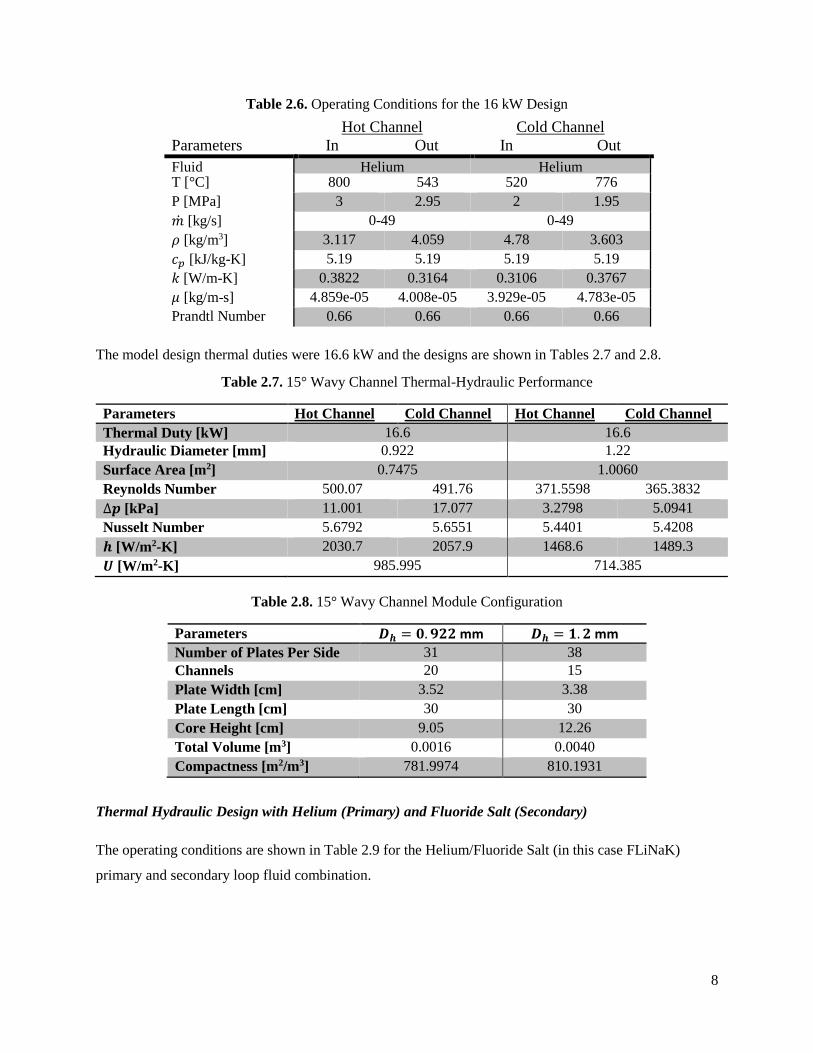
The model design thermal duties were 16.6 kW and the designs are shown in Tables 2.7 and 2.8.
Table 2.7. 15° Wavy Channel Thermal-Hydraulic Performance
Parameters Hot Channel Cold Channel Hot Channel Cold Channel
Thermal Duty [kW] 16.6 16.6
Hydraulic Diameter [mm] 0.922 1.22
Surface Area [m2] 0.7475 1.0060
Reynolds Number 500.07 491.76 371.5598 365.3832
∆𝒑 [kPa] 11.001 17.077 3.2798 5.0941
Nusselt Number 5.6792 5.6551 5.4401 5.4208
𝒉 [W/m2-K] 2030.7 2057.9 1468.6 1489.3
𝑼 [W/m2-K] 985.995 714.385
Table 2.8. 15° Wavy Channel Module Configuration
Parameters 𝑫𝒉 = 𝟎. 𝟗𝟐𝟐 mm 𝑫𝒉 = 𝟏. 𝟐 mm
Number of Plates Per Side 31 38
Channels 20 15
Plate Width [cm] 3.52 3.38
Plate Length [cm] 30 30
Core Height [cm] 9.05 12.26
Total Volume [m3] 0.0016 0.0040
Compactness [m2/m3] 781.9974 810.1931
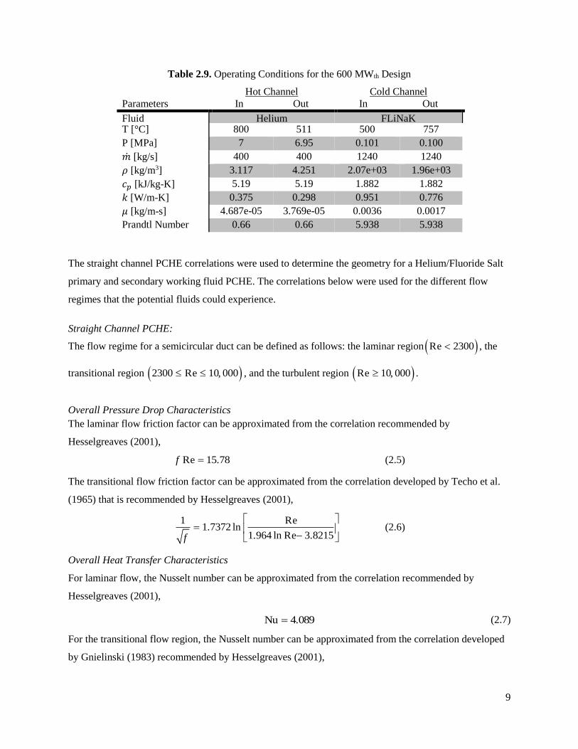
Thermal Hydraulic Design with Helium (Primary) and Fluoride Salt (Secondary)
The operating conditions are shown in Table 2.9 for the Helium/Fluoride Salt (in this case FLiNaK)
primary and secondary loop fluid combination.
9
Table 2.9. Operating Conditions for the 600 MWth Design
Parameters
Hot Channel
In Out
Cold Channel
In Out
Fluid Helium FLiNaK T [°C] 800 511 500 757
P [MPa] 7 6.95 0.101 0.100
�̇� [kg/s] 400 400 1240 1240
𝜌 [kg/m3] 3.117 4.251 2.07e+03 1.96e+03
𝑐𝑝 [kJ/kg-K] 5.19 5.19 1.882 1.882
𝑘 [W/m-K] 0.375 0.298 0.951 0.776
𝜇 [kg/m-s] 4.687e-05 3.769e-05 0.0036 0.0017
Prandtl Number 0.66 0.66 5.938 5.938
The straight channel PCHE correlations were used to determine the geometry for a Helium/Fluoride Salt
primary and secondary working fluid PCHE. The correlations below were used for the different flow
regimes that the potential fluids could experience.
Straight Channel PCHE:
The flow regime for a semicircular duct can be defined as follows: the laminar region Re 2300 , the
transitional region 2300 Re 10, 000 , and the turbulent region Re 10, 000 .
Overall Pressure Drop Characteristics
The laminar flow friction factor can be approximated from the correlation recommended by
Hesselgreaves (2001),
Re 15.78f (2.5)
The transitional flow friction factor can be approximated from the correlation developed by Techo et al.
(1965) that is recommended by Hesselgreaves (2001),
1 Re1.7372 ln
1.964 ln Re 3.8215f
(2.6)
Overall Heat Transfer Characteristics
For laminar flow, the Nusselt number can be approximated from the correlation recommended by
Hesselgreaves (2001),
Nu 4.089 (2.7)
For the transitional flow region, the Nusselt number can be approximated from the correlation developed
by Gnielinski (1983) recommended by Hesselgreaves (2001),
10
2
3
20.5
3
2 Re 1000 P rNu 1
1 12.7 2 P r 1
hf d
Lf
(2.8)
This correlation is valid from 42300 Re 5 10 and 0.5 Pr 2000 .
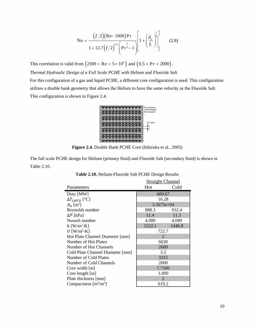
Thermal Hydraulic Design of a Full Scale PCHE with Helium and Fluoride Salt
For this configuration of a gas and liquid PCHE, a different core configuration is used. This configuration
utilizes a double bank geometry that allows the Helium to have the same velocity as the Fluoride Salt.
This configuration is shown in Figure 2.4.
Figure 2.4. Double Bank PCHE Core (Ishizuka et al., 2005)
The full scale PCHE design for Helium (primary fluid) and Fluoride Salt (secondary fluid) is shown in
Table 2.10.
Table 2.10. Helium-Fluoride Salt PCHE Design Results
Parameters
Straight Channel
Hot Cold
Duty [MW] 600.67
∆𝑇𝐿𝑀𝑇𝐷 [°C] 16.28
𝐴ℎ [m2] 3.5675e+04
Reynolds number 888.3 932.4
∆𝑃 [kPa] 11.4 11.3
Nusselt number 4.089 4.089
ℎ [W/m2-K] 1522.1 1446.8
𝑈 [W/m2-K] 722.7
Hot Plate Channel Diameter [mm] 2
Number of Hot Plates 6630
Number of Hot Channels 2600
Cold Plate Channel Diameter [mm] 3.5
Number of Cold Plates 3315
Number of Cold Channels 2000
Core width [m] 7.7500
Core length [m] 1.000
Plate thickness [mm] 2
Compactness [m2/m3] 619.2
11
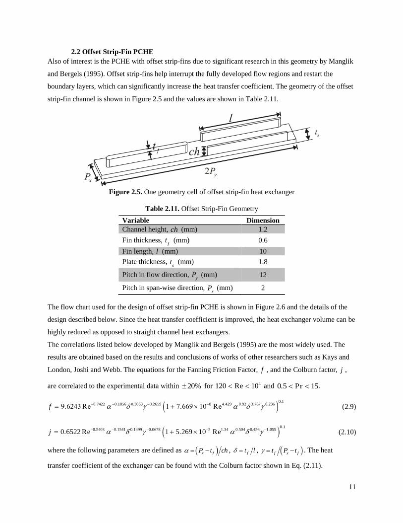
2.2 Offset Strip-Fin PCHE
Also of interest is the PCHE with offset strip-fins due to significant research in this geometry by Manglik
and Bergels (1995). Offset strip-fins help interrupt the fully developed flow regions and restart the
boundary layers, which can significantly increase the heat transfer coefficient. The geometry of the offset
strip-fin channel is shown in Figure 2.5 and the values are shown in Table 2.11.
Figure 2.5. One geometry cell of offset strip-fin heat exchanger
Table 2.11. Offset Strip-Fin Geometry
Variable Dimension
Channel height, ch (mm) 1.2
Fin thickness, f
t (mm) 0.6
Fin length, l (mm) 10
Plate thickness, s
t (mm) 1.8
Pitch in flow direction, y
P (mm) 12
Pitch in span-wise direction, x
P (mm) 2
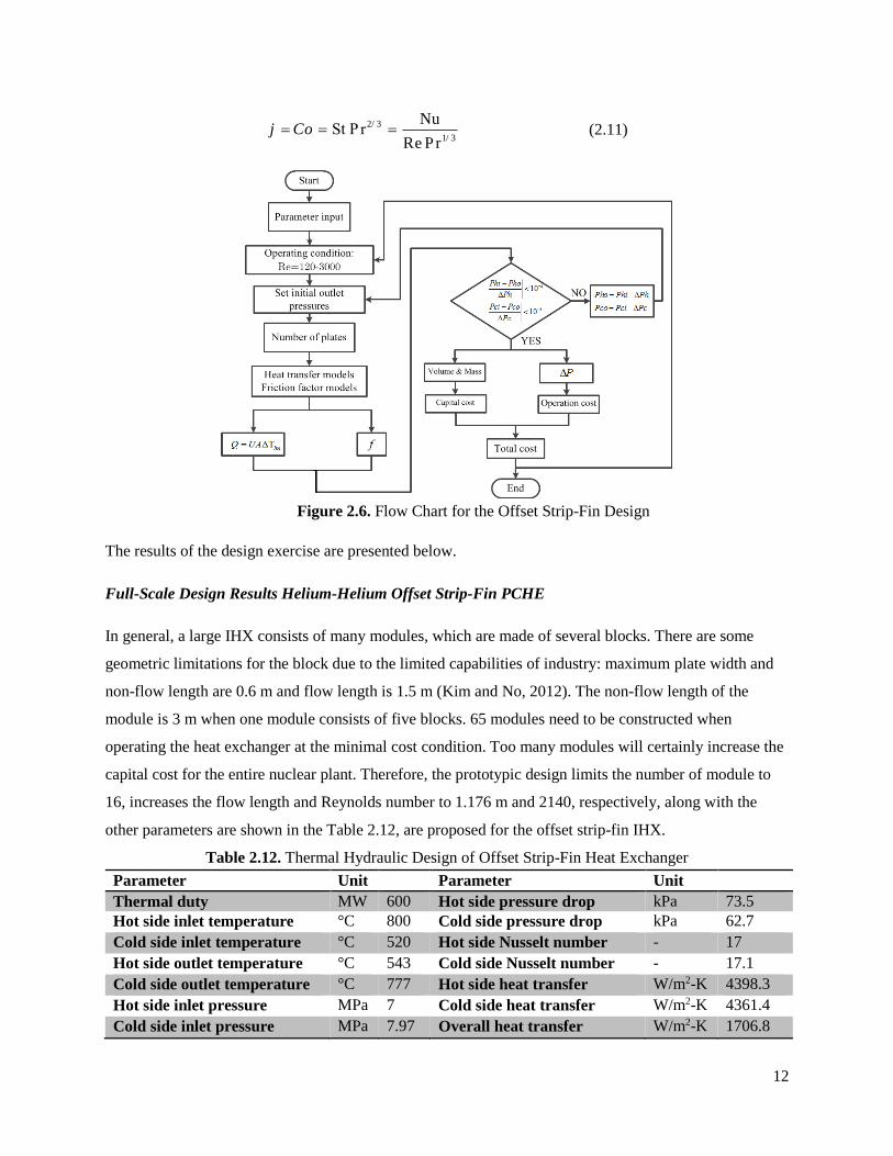
The flow chart used for the design of offset strip-fin PCHE is shown in Figure 2.6 and the details of the
design described below. Since the heat transfer coefficient is improved, the heat exchanger volume can be
highly reduced as opposed to straight channel heat exchangers.
The correlations listed below developed by Manglik and Bergels (1995) are the most widely used. The
results are obtained based on the results and conclusions of works of other researchers such as Kays and
London, Joshi and Webb. The equations for the Fanning Friction Factor, f , and the Colburn factor, j ,
are correlated to the experimental data within 20% for 4120 Re 10 and 0.5 Pr 15 .
0.1
0.7422 0.1856 0.3053 0.2659 8 4.429 0.92 3.767 0.2369.6243Re 1 7.669 10 Re f (2.9)
0.1
0.5403 0.1541 0.1499 0.0678 5 1.34 0.504 0.456 1.0550.6522 Re 1 5.269 10 Rej (2.10)
where the following parameters are defined as x fP t ch , ft l , f x ft P t . The heat
transfer coefficient of the exchanger can be found with the Colburn factor shown in Eq. (2.11).
12
2/ 3
1/ 3
NuSt Pr
Re Prj Co (2.11)
Figure 2.6. Flow Chart for the Offset Strip-Fin Design
The results of the design exercise are presented below.
Full-Scale Design Results Helium-Helium Offset Strip-Fin PCHE
In general, a large IHX consists of many modules, which are made of several blocks. There are some
geometric limitations for the block due to the limited capabilities of industry: maximum plate width and
non-flow length are 0.6 m and flow length is 1.5 m (Kim and No, 2012). The non-flow length of the
module is 3 m when one module consists of five blocks. 65 modules need to be constructed when
operating the heat exchanger at the minimal cost condition. Too many modules will certainly increase the
capital cost for the entire nuclear plant. Therefore, the prototypic design limits the number of module to
16, increases the flow length and Reynolds number to 1.176 m and 2140, respectively, along with the
other parameters are shown in the Table 2.12, are proposed for the offset strip-fin IHX.
Table 2.12. Thermal Hydraulic Design of Offset Strip-Fin Heat Exchanger
Parameter Unit Parameter Unit
Thermal duty MW 600 Hot side pressure drop kPa 73.5
Hot side inlet temperature °C 800 Cold side pressure drop kPa 62.7
Cold side inlet temperature °C 520 Hot side Nusselt number - 17
Hot side outlet temperature °C 543 Cold side Nusselt number - 17.1
Cold side outlet temperature °C 777 Hot side heat transfer
coefficient
W/m2-K 4398.3
Hot side inlet pressure MPa 7 Cold side heat transfer
coefficient
W/m2-K 4361.4
Cold side inlet pressure MPa 7.97 Overall heat transfer
coefficient
W/m2-K 1706.8

13
Hot side Reynolds number - 2140 LMTD °C 23
Cold side Reynolds number - 2174 Total plate number - 26669
Hot side mean velocity m/s 17.8 Surface area density m2 /m3 892
Cold side mean velocity m/s 15.3 Flow length m 1.176
Hot side hydraulic diameter mm 1.3 Total module number - 16
Cold side hydraulic diameter mm 1.3 Volume m3 33.9
Prototype Design Results Helium-Helium Offset Strip-Fin PCHE
The volume of prototypic offset strip-fin IHX is more than 30 m3 for a 600 MWth-Reactor. It is important
to know the IHX thermal-hydraulics performance from the test experiment. However, doing experiment
with prototype is very expensive and time consuming. In order to get the IHX’s thermal-hydraulics
performance and verify its abilities for NGNP, a scaling-down approach, which is the method that can
reduce the volume of the test heat exchanger with the similar performance as prototype, was adopted in
this design.
For this study, the main purpose of scaling down the IHX was to ensure the flow and heat transfer
mechanisms of the IHX test model were same as that of prototypical IHX, which means to keep the
Reynolds number of the IHX test model similar to that of prototype. The Reynolds number can be
obtained from the energy balance equations.
pmc T Q (2.12)
lmUA T Q (2.13)
From Eq. (2.12) and (2.13), the Reynolds number ratio of the test model to prototypic IHX can be
expressed as Eq. (2.14).
Re lm
RR R
L Tvd
T
(2.14)
In order to keep the mechanisms of test model are same as the prototypical IHX, the Reynolds number
ratio should be approximately equal to one. From Eq. (2.14), only by adjusting lm
T and T can the
Reynolds numbers for both test model and prototype is kept the same, since the flow length of the test
model is much smaller than the length of prototype. It is important to note that densities of fluid for
prototypical and test model are very different due to fact that pressure in the exiting experimental facility
cannot exceed 3 MPa.
The main purpose of this project is to determine the performance of IHX at high temperature condition, so
the hot side inlet temperature was maintained at 800°C for the scaled-down IHX. The flow length was
chosen to be about 0.3 m due to the limitation of facility and flexibility for installation. In all, one
14
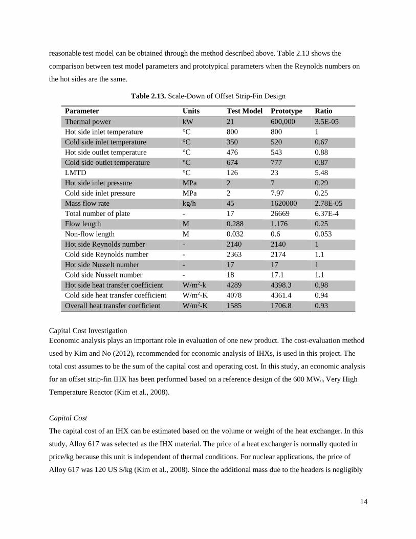
reasonable test model can be obtained through the method described above. Table 2.13 shows the
comparison between test model parameters and prototypical parameters when the Reynolds numbers on
the hot sides are the same.
Table 2.13. Scale-Down of Offset Strip-Fin Design
Parameter Units Test Model Prototype Ratio
Thermal power kW 21 600,000 3.5E-05
Hot side inlet temperature °C 800 800 1
Cold side inlet temperature °C 350 520 0.67
Hot side outlet temperature °C 476 543 0.88
Cold side outlet temperature °C 674 777 0.87
LMTD °C 126 23 5.48
Hot side inlet pressure MPa 2 7 0.29
Cold side inlet pressure MPa 2 7.97 0.25
Mass flow rate kg/h 45 1620000 2.78E-05
Total number of plate - 17 26669 6.37E-4
Flow length M 0.288 1.176 0.25
Non-flow length M 0.032 0.6 0.053
Hot side Reynolds number - 2140 2140 1
Cold side Reynolds number - 2363 2174 1.1
Hot side Nusselt number - 17 17 1
Cold side Nusselt number - 18 17.1 1.1
Hot side heat transfer coefficient W/m2-k 4289 4398.3 0.98
Cold side heat transfer coefficient W/m2-K 4078 4361.4 0.94
Overall heat transfer coefficient W/m2-K 1585 1706.8 0.93
Capital Cost Investigation
Economic analysis plays an important role in evaluation of one new product. The cost-evaluation method
used by Kim and No (2012), recommended for economic analysis of IHXs, is used in this project. The
total cost assumes to be the sum of the capital cost and operating cost. In this study, an economic analysis
for an offset strip-fin IHX has been performed based on a reference design of the 600 MWth Very High
Temperature Reactor (Kim et al., 2008).
Capital Cost
The capital cost of an IHX can be estimated based on the volume or weight of the heat exchanger. In this
study, Alloy 617 was selected as the IHX material. The price of a heat exchanger is normally quoted in
price/kg because this unit is independent of thermal conditions. For nuclear applications, the price of
Alloy 617 was 120 US $/kg (Kim et al., 2008). Since the additional mass due to the headers is negligibly
15
small and was neglected, the capital cost can be obtained by multiplying the material cost m
C and the IHX
core volume V by the metal density as:
c mC C V (2.15)
Capital cost is a one-time expense incurred on the purchase of equipment. Since the unit of the capital
cost ($) is different from that of the operating cost ($/y), it is necessary to convert the unit of capital cost
($) to that of operating cost ($/y) by taking into account bank interest rate and IHX lifetime. If a loan from
a bank with interest r and after n years, the total payment ct
C is:
(1 )n
ct cC C r (2.16)
Assume a constant payback is made to the bank then the payment cp
C for every year can be calculated as:
1
1
(1 ) (1 ) 1i n
cpi n
ct cpi
CC C r r
r
(2.17)
Operating Cost
Operating cost for IHXs is proportional to the pumping power, which can be determined by the pressure
drop across the IHX:
pump
m pP
(2.18)
where 𝜂 is the pump efficiency, in general, 𝜂 = 0.80 − 0.85, m is the mass flow rate. The electricity cost
eC can be obtained from the U.S. Energy Information Administration for the industrial sector. So the
operating cost o
C can be assessed as:
pumpo eC C P (2.19)
Total Cost
As described above, the total cost of IHX is the summation of the capital cost and operating cost. The
reference-operating period for IHXs is assumed to be 20 years, and the interest rate of a bank is assumed
to be 5% (Kim and No, 2012). Then the total cost can be obtained from:
t cp oC C C (2.20)
Effects of Geometric Parameters of Offset Strip-Fin PCHEs
To get reasonable geometric parameters of offset strip-fin IHXs, geometric parameters evaluations were
performed based on the economic analysis described above. Five geometry parameters were evaluated,
16
namely, pitch in span-wise direction, pitch in flow direction, fin height, fin length, and fin thickness. In
the first calculation, five geometric parameters were selected from Losier et al. (2007), which were
evaluated by the CFD calculations. Table 2.13 lists the geometric parameters for both prototypic design
and test model design which were obtained by iterating the cost-evaluation process with only one
parameter changing per iteration.
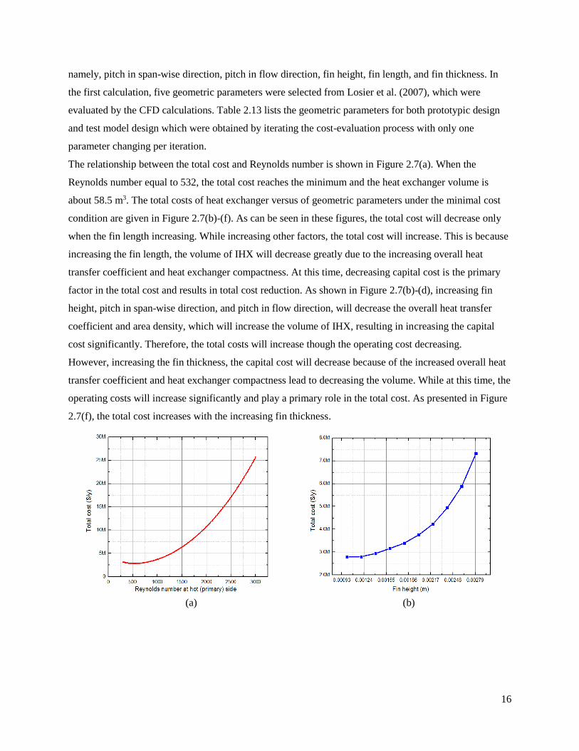
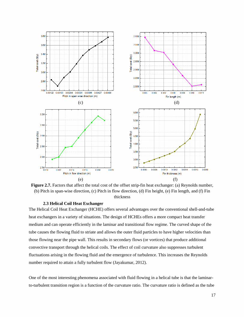
The relationship between the total cost and Reynolds number is shown in Figure 2.7(a). When the
Reynolds number equal to 532, the total cost reaches the minimum and the heat exchanger volume is
about 58.5 m3. The total costs of heat exchanger versus of geometric parameters under the minimal cost
condition are given in Figure 2.7(b)-(f). As can be seen in these figures, the total cost will decrease only
when the fin length increasing. While increasing other factors, the total cost will increase. This is because
increasing the fin length, the volume of IHX will decrease greatly due to the increasing overall heat
transfer coefficient and heat exchanger compactness. At this time, decreasing capital cost is the primary
factor in the total cost and results in total cost reduction. As shown in Figure 2.7(b)-(d), increasing fin
height, pitch in span-wise direction, and pitch in flow direction, will decrease the overall heat transfer
coefficient and area density, which will increase the volume of IHX, resulting in increasing the capital
cost significantly. Therefore, the total costs will increase though the operating cost decreasing.
However, increasing the fin thickness, the capital cost will decrease because of the increased overall heat
transfer coefficient and heat exchanger compactness lead to decreasing the volume. While at this time, the
operating costs will increase significantly and play a primary role in the total cost. As presented in Figure
2.7(f), the total cost increases with the increasing fin thickness.
(a) (b)
17
(c) (d)
(e) (f)
Figure 2.7. Factors that affect the total cost of the offset strip-fin heat exchanger: (a) Reynolds number,
(b) Pitch in span-wise direction, (c) Pitch in flow direction, (d) Fin height, (e) Fin length, and (f) Fin
thickness
2.3 Helical Coil Heat Exchanger
The Helical Coil Heat Exchanger (HCHE) offers several advantages over the conventional shell-and-tube
heat exchangers in a variety of situations. The design of HCHEs offers a more compact heat transfer
medium and can operate efficiently in the laminar and transitional flow regime. The curved shape of the
tube causes the flowing fluid to striate and allows the outer fluid particles to have higher velocities than
those flowing near the pipe wall. This results in secondary flows (or vortices) that produce additional
convective transport through the helical coils. The effect of coil curvature also suppresses turbulent
fluctuations arising in the flowing fluid and the emergence of turbulence. This increases the Reynolds
number required to attain a fully turbulent flow (Jayakumar, 2012).
One of the most interesting phenomena associated with fluid flowing in a helical tube is that the laminar-
to-turbulent transition region is a function of the curvature ratio. The curvature ratio is defined as the tube

18
radius divided by the radius curvature and influences the critical Reynolds number at which point the
laminar flow regime begins its transitions to the turbulent flow regime. Figure 2.8 shows the influence of
curvature ratio on the critical Reynolds number for HCHEs.
Figure 2.8. Critical Reynolds number as a function of Curvature Ratio (Jayakumar, 2012)
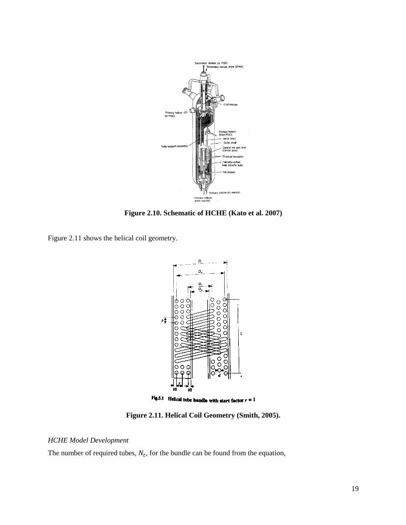
Figure 2.9 shows one such HCHE design for an IHX for the very high/high temperature reactor. Figure
2.10 shows an interior view of the HCHE and tube bundle orientation. The inner annulus of the exchanger
allows the primary fluid to flow and gives a better temperature control for transient situations.
Figure 2.9. Diagram of HCHE bundle (Kato et al. 2007)
19
Figure 2.10. Schematic of HCHE (Kato et al. 2007)
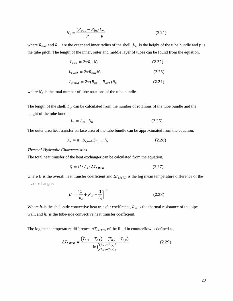
Figure 2.11 shows the helical coil geometry.
Figure 2.11. Helical Coil Geometry (Smith, 2005).
HCHE Model Development
The number of required tubes, 𝑁𝑡, for the bundle can be found from the equation,
20
𝑁𝑡 =(𝑅𝑜𝑢𝑡 − 𝑅𝑖𝑛)
𝑝
𝐿𝑚
𝑝 (2.21)
where 𝑅𝑜𝑢𝑡 and 𝑅𝑖𝑛 are the outer and inner radius of the shell, 𝐿𝑚 is the height of the tube bundle and 𝑝 is
the tube pitch. The length of the inner, outer and middle layer of tubes can be found from the equation,
𝐿𝑡,𝑖𝑛 = 2𝜋𝑅𝑖𝑛𝑁𝑏 (2.22)
𝐿𝑡,𝑜𝑢𝑡 = 2𝜋𝑅𝑜𝑢𝑡𝑁𝑏 (2.23)
𝐿𝑡,𝑚𝑖𝑑 = 2𝜋(𝑅𝑖𝑛 + 𝑅𝑜𝑢𝑡)𝑁𝑏 (2.24)
where 𝑁𝑏 is the total number of tube rotations of the tube bundle.
The length of the shell, 𝐿𝑠, can be calculated from the number of rotations of the tube bundle and the
height of the tube bundle.
𝐿𝑠 = 𝐿𝑚 ∙ 𝑁𝑏 (2.25)
The outer area heat transfer surface area of the tube bundle can be approximated from the equation,
𝐴𝑠 = 𝜋 ∙ 𝐷𝑡,𝑜𝑢𝑡∙𝐿𝑡,𝑚𝑖𝑑∙𝑁𝑡 (2.26)
Thermal-Hydraulic Characteristics
The total heat transfer of the heat exchanger can be calculated from the equation,
𝑄 = 𝑈 ∙ 𝐴𝑠 ∙ ∆𝑇𝐿𝑀𝑇𝐷 (2.27)
where 𝑈 is the overall heat transfer coefficient and ∆𝑇𝐿𝑀𝑇𝐷 is the log mean temperature difference of the
heat exchanger.
𝑈 = [1
ℎ𝑠+ 𝑅𝑤 +
1
ℎ𝑡]
−1
(2.28)
Where ℎ𝑠is the shell-side convective heat transfer coefficient, 𝑅𝑤 is the thermal resistance of the pipe
wall, and ℎ𝑡 is the tube-side convective heat transfer coefficient.
The log mean temperature difference, ∆𝑇𝐿𝑀𝑇𝐷, of the fluid in counterflow is defined as,
∆𝑇𝐿𝑀𝑇𝐷 =(𝑇ℎ,1 − 𝑇𝑐,1) − (𝑇ℎ,2 − 𝑇𝑐,2)
ln ((𝑇ℎ,1−𝑇𝑐,1)
(𝑇ℎ,2−𝑇𝑐,2))
(2.29)
21
The counterflow fluid orientation for the HCHE is chosen because it utilizes a larger temperature
difference and results in a closer temperature approach and higher temperature effectiveness than heat
exchangers in concurrent flow.
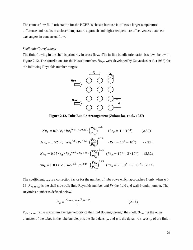
Shell-side Correlations:
The fluid flowing in the shell is primarily in cross flow. The in-line bundle orientation is shown below in
Figure 2.12. The correlations for the Nusselt number, 𝑁𝑢𝑏, were developed by Zukauskas et al. (1987) for
the following Reynolds number ranges:
Figure 2.12. Tube Bundle Arrangement (Zukauskas et al., 1987)
𝑁𝑢𝑏 = 0.9 ∙ 𝑐𝑛 ∙ 𝑅𝑒𝑏0.4 ∙ 𝑃𝑟0.36 ∙ (
𝑃𝑟𝑏
𝑃𝑟𝑤)
0.25
(𝑅𝑒𝑏 = 1 − 102) (2.30)
𝑁𝑢𝑏 = 0.52 ∙ 𝑐𝑛 ∙ 𝑅𝑒𝑏0.4 ∙ 𝑃𝑟0.36 ∙ (
𝑃𝑟𝑏
𝑃𝑟𝑤)
0.25
(𝑅𝑒𝑏 = 102 − 103) (2.31)
𝑁𝑢𝑏 = 0.27 ∙ 𝑐𝑛 ∙ 𝑅𝑒𝑏0.62 ∙ 𝑃𝑟0.36 ∙ (
𝑃𝑟𝑏
𝑃𝑟𝑤)
0.25
(𝑅𝑒𝑏 = 103 − 2 ∙ 105) (2.32)
𝑁𝑢𝑏 = 0.033 ∙ 𝑐𝑛 ∙ 𝑅𝑒𝑏0.8 ∙ 𝑃𝑟0.36 ∙ (
𝑃𝑟𝑏
𝑃𝑟𝑤)
0.25
(𝑅𝑒𝑏 = 2 ∙ 105 − 2 ∙ 106) 2.33)
The coefficient, 𝑐𝑛, is a correction factor for the number of tube rows which approaches 1 only when 𝑛 >
16. 𝑅𝑒𝑠ℎ𝑒𝑙𝑙,𝑏 is the shell-side bulk fluid Reynolds number and 𝑃𝑟 the fluid and wall Prandtl number. The
Reynolds number is defined below.
𝑅𝑒𝑏 =𝑉𝑠ℎ𝑒𝑙𝑙,𝑚𝑎𝑥𝐷𝑡,𝑜𝑢𝑡𝜌
𝜇 (2.34)
𝑉𝑠ℎ𝑒𝑙𝑙,𝑚𝑎𝑥 is the maximum average velocity of the fluid flowing through the shell, 𝐷𝑡,𝑜𝑢𝑡 is the outer
diameter of the tubes in the tube bundle, 𝜌 is the fluid density, and 𝜇 is the dynamic viscosity of the fluid.
22
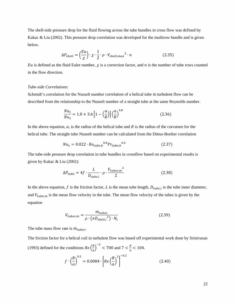
The shell-side pressure drop for the fluid flowing across the tube bundles in cross flow was defined by
Kakac & Liu (2002). This pressure drop correlation was developed for the multirow bundle and is given
below.
∆𝑃𝑠ℎ𝑒𝑙𝑙 = (𝐸𝑢
𝜒) ∙ 𝜒 ∙
1
2∙ 𝜌 ∙ 𝑉𝑠ℎ𝑒𝑙𝑙,𝑚𝑎𝑥
2 ∙ 𝑛 (2.35)
𝐸𝑢 is defined as the fluid Euler number, 𝜒 is a correction factor, and 𝑛 is the number of tube rows counted
in the flow direction.
Tube-side Correlations:
Schmidt’s correlation for the Nusselt number correlation of a helical tube in turbulent flow can be
described from the relationship to the Nusselt number of a straight tube at the same Reynolds number.
𝑁𝑢𝑡
𝑁𝑢𝑠= 1.0 + 3.6 [1 − (
𝑎
𝑅)] (
𝑎
𝑅)
0.8
(2.36)
In the above equation, 𝑎, is the radius of the helical tube and 𝑅 is the radius of the curvature for the
helical tube. The straight tube Nusselt number can be calculated from the Dittus-Boelter correlation
𝑁𝑢𝑠 = 0.022 ∙ 𝑅𝑒𝑡𝑢𝑏𝑒,𝑏0.8𝑃𝑟𝑡𝑢𝑏𝑒,𝑏
0.5 (2.37)
The tube-side pressure drop correlation in tube bundles in crossflow based on experimental results is
given by Kakac & Liu (2002):
∆𝑃𝑡𝑢𝑏𝑒 = 4𝑓 ∙𝐿
𝐷𝑡𝑢𝑏𝑒,𝑖∙ 𝜌 ∙
𝑉𝑡𝑢𝑏𝑒𝑠,𝑚2
2 (2.38)
In the above equation, 𝑓 is the friction factor, 𝐿 is the mean tube length, 𝐷𝑡𝑢𝑏𝑒,𝑖 is the tube inner diameter,
and 𝑉𝑡𝑢𝑏𝑒,𝑚 is the mean flow velocity in the tube. The mean flow velocity of the tubes is given by the
equation
𝑉𝑡𝑢𝑏𝑒𝑠,𝑚 =�̇�𝑡𝑢𝑏𝑒𝑠
𝜌 ∙ (𝜋𝐷𝑠ℎ𝑒𝑙𝑙,𝑖2) ∙ 𝑁𝑡
(2.39)
The tube mass flow rate is �̇�𝑡𝑢𝑏𝑒𝑠.
The friction factor for a helical coil in turbulent flow was based off experimental work done by Srinivasan
(1993) defined for the conditions 𝑅𝑒 (𝑅
𝑎)
−2< 700 and 7 <
𝑅
𝑎< 104.
𝑓 ∙ (𝑅
𝑎)
0.5
= 0.0084 ∙ [𝑅𝑒 (𝑅
𝑎)
2
]
−0.2
(2.40)
23
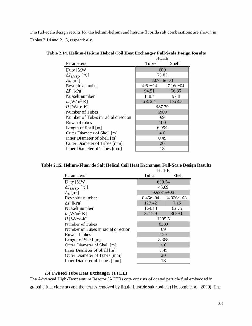
The full-scale design results for the helium-helium and helium-fluoride salt combinations are shown in
Tables 2.14 and 2.15, respectively.
Table 2.14. Helium-Helium Helical Coil Heat Exchanger Full-Scale Design Results
Parameters
HCHE
Tubes Shell
Duty [MW] 600
∆𝑇𝐿𝑀𝑇𝐷 [°C] 75.85
𝐴ℎ [m2] 8.0734e+03
Reynolds number 4.6e+04 7.16e+04
∆𝑃 [kPa] 94.51 66.86
Nusselt number 148.4 97.8
ℎ [W/m2-K] 2813.4 1728.7
𝑈 [W/m2-K] 987.79
Number of Tubes 6900
Number of Tubes in radial direction 69
Rows of tubes 100
Length of Shell [m] 6.990
Outer Diameter of Shell [m] 4.6
Inner Diameter of Shell [m] 0.49
Outer Diameter of Tubes [mm] 20
Inner Diameter of Tubes [mm] 18
Table 2.15. Helium-Fluoride Salt Helical Coil Heat Exchanger Full-Scale Design Results
Parameters
HCHE
Tubes Shell
Duty [MW] 609.54
∆𝑇𝐿𝑀𝑇𝐷 [°C] 45.09
𝐴ℎ [m2] 9.6881e+03
Reynolds number 8.46e+04 4.036e+03
∆𝑃 [kPa] 127.42 7.15
Nusselt number 169.48 62.75
ℎ [W/m2-K] 3212.9 3059.0
𝑈 [W/m2-K] 1395.5
Number of Tubes 8280
Number of Tubes in radial direction 69
Rows of tubes 120
Length of Shell [m] 8.388
Outer Diameter of Shell [m] 4.6
Inner Diameter of Shell [m] 0.49
Outer Diameter of Tubes [mm] 20
Inner Diameter of Tubes [mm] 18
2.4 Twisted Tube Heat Exchanger (TTHE)
The Advanced High-Temperature Reactor (AHTR) core consists of coated particle fuel embedded in
graphite fuel elements and the heat is removed by liquid fluoride salt coolant (Holcomb et al., 2009). The
24
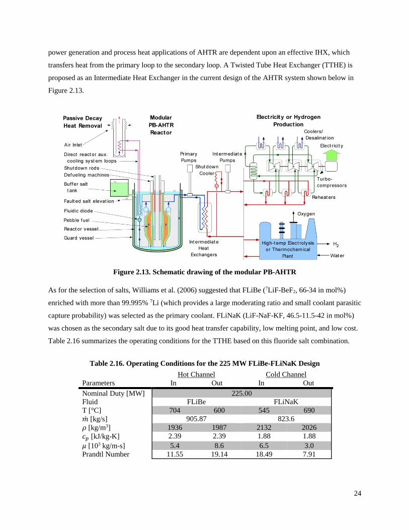
power generation and process heat applications of AHTR are dependent upon an effective IHX, which
transfers heat from the primary loop to the secondary loop. A Twisted Tube Heat Exchanger (TTHE) is
proposed as an Intermediate Heat Exchanger in the current design of the AHTR system shown below in
Figure 2.13.
Figure 2.13. Schematic drawing of the modular PB-AHTR
As for the selection of salts, Williams et al. (2006) suggested that FLiBe (7LiF-BeF2, 66-34 in mol%)
enriched with more than 99.995% 7Li (which provides a large moderating ratio and small coolant parasitic
capture probability) was selected as the primary coolant. FLiNaK (LiF-NaF-KF, 46.5-11.5-42 in mol%)
was chosen as the secondary salt due to its good heat transfer capability, low melting point, and low cost.
Table 2.16 summarizes the operating conditions for the TTHE based on this fluoride salt combination.
Table 2.16. Operating Conditions for the 225 MW FLiBe-FLiNaK Design
Parameters
Hot Channel
In Out
Cold Channel
In Out
Nominal Duty [MW] 225.00
Fluid FLiBe FLiNaK
T [°C] 704 600 545 690
�̇� [kg/s] 905.87 823.6
𝜌 [kg/m3] 1936 1987 2132 2026
𝑐𝑝 [kJ/kg-K] 2.39 2.39 1.88 1.88
𝜇 [103 kg/m-s] 5.4 8.6 6.5 3.0
Prandtl Number 11.55 19.14 18.49 7.91
25
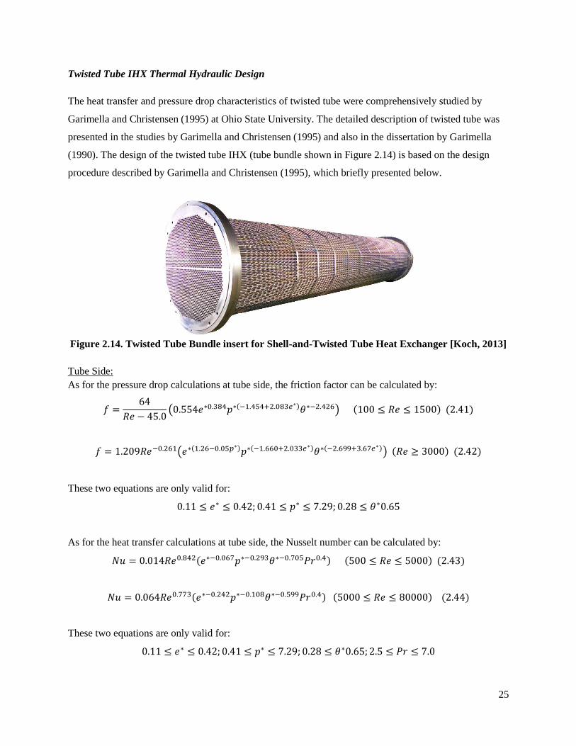
Twisted Tube IHX Thermal Hydraulic Design
The heat transfer and pressure drop characteristics of twisted tube were comprehensively studied by
Garimella and Christensen (1995) at Ohio State University. The detailed description of twisted tube was
presented in the studies by Garimella and Christensen (1995) and also in the dissertation by Garimella
(1990). The design of the twisted tube IHX (tube bundle shown in Figure 2.14) is based on the design
procedure described by Garimella and Christensen (1995), which briefly presented below.
Figure 2.14. Twisted Tube Bundle insert for Shell-and-Twisted Tube Heat Exchanger [Koch, 2013]
Tube Side:
As for the pressure drop calculations at tube side, the friction factor can be calculated by:
𝑓 =64
𝑅𝑒 − 45.0(0.554𝑒∗0.384𝑝∗(−1.454+2.083𝑒∗)𝜃∗−2.426) (100 ≤ 𝑅𝑒 ≤ 1500) (2.41)
𝑓 = 1.209𝑅𝑒−0.261(𝑒∗(1.26−0.05𝑝∗)𝑝∗(−1.660+2.033𝑒∗)𝜃∗(−2.699+3.67𝑒∗)) (𝑅𝑒 ≥ 3000) (2.42)
These two equations are only valid for:
0.11 ≤ 𝑒∗ ≤ 0.42; 0.41 ≤ 𝑝∗ ≤ 7.29; 0.28 ≤ 𝜃∗0.65
As for the heat transfer calculations at tube side, the Nusselt number can be calculated by:
𝑁𝑢 = 0.014𝑅𝑒0.842(𝑒∗−0.067𝑝∗−0.293𝜃∗−0.705𝑃𝑟0.4) (500 ≤ 𝑅𝑒 ≤ 5000) (2.43)
𝑁𝑢 = 0.064𝑅𝑒0.773(𝑒∗−0.242𝑝∗−0.108𝜃∗−0.599𝑃𝑟0.4) (5000 ≤ 𝑅𝑒 ≤ 80000) (2.44)
These two equations are only valid for:
0.11 ≤ 𝑒∗ ≤ 0.42; 0.41 ≤ 𝑝∗ ≤ 7.29; 0.28 ≤ 𝜃∗0.65; 2.5 ≤ 𝑃𝑟 ≤ 7.0
26
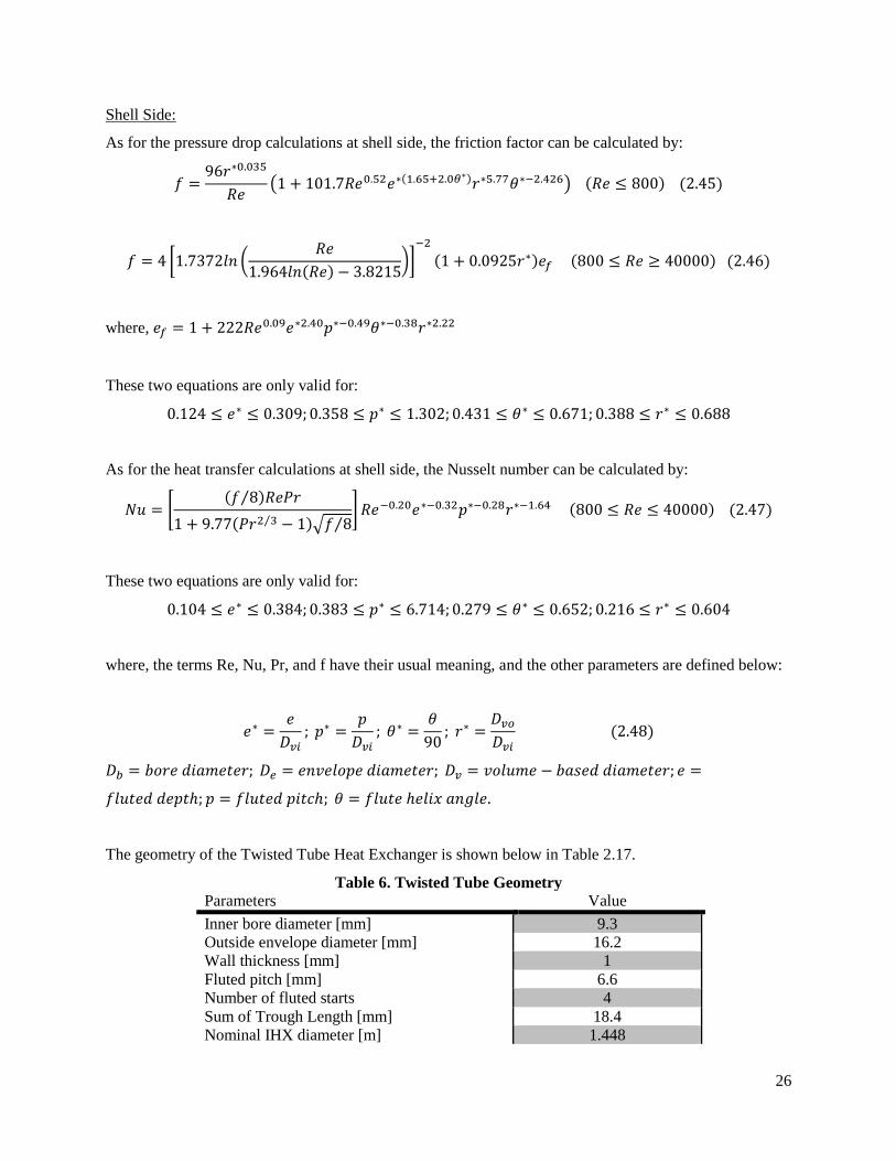
Shell Side:
As for the pressure drop calculations at shell side, the friction factor can be calculated by:
𝑓 =96𝑟∗0.035
𝑅𝑒(1 + 101.7𝑅𝑒0.52𝑒∗(1.65+2.0𝜃∗)𝑟∗5.77𝜃∗−2.426) (𝑅𝑒 ≤ 800) (2.45)
𝑓 = 4 [1.7372𝑙𝑛 (𝑅𝑒
1.964𝑙𝑛(𝑅𝑒) − 3.8215)]
−2
(1 + 0.0925𝑟∗)𝑒𝑓 (800 ≤ 𝑅𝑒 ≥ 40000) (2.46)
where, 𝑒𝑓 = 1 + 222𝑅𝑒0.09𝑒∗2.40𝑝∗−0.49𝜃∗−0.38𝑟∗2.22
These two equations are only valid for:
0.124 ≤ 𝑒∗ ≤ 0.309; 0.358 ≤ 𝑝∗ ≤ 1.302; 0.431 ≤ 𝜃∗ ≤ 0.671; 0.388 ≤ 𝑟∗ ≤ 0.688
As for the heat transfer calculations at shell side, the Nusselt number can be calculated by:
𝑁𝑢 = [(𝑓 8⁄ )𝑅𝑒𝑃𝑟
1 + 9.77(𝑃𝑟2 3⁄ − 1)√𝑓 8⁄] 𝑅𝑒−0.20𝑒∗−0.32𝑝∗−0.28𝑟∗−1.64 (800 ≤ 𝑅𝑒 ≤ 40000) (2.47)
These two equations are only valid for:
0.104 ≤ 𝑒∗ ≤ 0.384; 0.383 ≤ 𝑝∗ ≤ 6.714; 0.279 ≤ 𝜃∗ ≤ 0.652; 0.216 ≤ 𝑟∗ ≤ 0.604
where, the terms Re, Nu, Pr, and f have their usual meaning, and the other parameters are defined below:
𝑒∗ =𝑒
𝐷𝑣𝑖; 𝑝∗ =
𝑝
𝐷𝑣𝑖; 𝜃∗ =
𝜃
90; 𝑟∗ =
𝐷𝑣𝑜
𝐷𝑣𝑖 (2.48)
𝐷𝑏 = 𝑏𝑜𝑟𝑒 𝑑𝑖𝑎𝑚𝑒𝑡𝑒𝑟; 𝐷𝑒 = 𝑒𝑛𝑣𝑒𝑙𝑜𝑝𝑒 𝑑𝑖𝑎𝑚𝑒𝑡𝑒𝑟; 𝐷𝑣 = 𝑣𝑜𝑙𝑢𝑚𝑒 − 𝑏𝑎𝑠𝑒𝑑 𝑑𝑖𝑎𝑚𝑒𝑡𝑒𝑟; 𝑒 =
𝑓𝑙𝑢𝑡𝑒𝑑 𝑑𝑒𝑝𝑡ℎ; 𝑝 = 𝑓𝑙𝑢𝑡𝑒𝑑 𝑝𝑖𝑡𝑐ℎ; 𝜃 = 𝑓𝑙𝑢𝑡𝑒 ℎ𝑒𝑙𝑖𝑥 𝑎𝑛𝑔𝑙𝑒.
The geometry of the Twisted Tube Heat Exchanger is shown below in Table 2.17.
Table 6. Twisted Tube Geometry
Parameters Value
Inner bore diameter [mm] 9.3
Outside envelope diameter [mm] 16.2
Wall thickness [mm] 1
Fluted pitch [mm] 6.6
Number of fluted starts 4
Sum of Trough Length [mm] 18.4
Nominal IHX diameter [m] 1.448
27
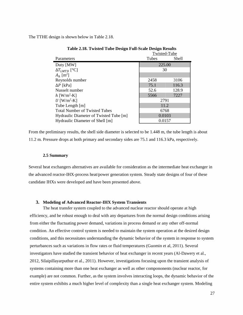
The TTHE design is shown below in Table 2.18.
Table 2.18. Twisted Tube Design Full-Scale Design Results
Parameters
Twisted-Tube
Tubes Shell
Duty [MW] 225.00
∆𝑇𝐿𝑀𝑇𝐷 [°C] 30
𝐴ℎ [m2]
Reynolds number 2458 3106
∆𝑃 [kPa] 75.1 116.3
Nusselt number 52.6 128.9
ℎ [W/m2-K] 5566 7227
𝑈 [W/m2-K] 2791
Tube Length [m] 11.2
Total Number of Twisted Tubes 6768
Hydraulic Diameter of Twisted Tube [m] 0.0103
Hydraulic Diameter of Shell [m] 0.0157
From the preliminary results, the shell side diameter is selected to be 1.448 m, the tube length is about
11.2 m. Pressure drops at both primary and secondary sides are 75.1 and 116.3 kPa, respectively.
2.5 Summary
Several heat exchangers alternatives are available for consideration as the intermediate heat exchanger in
the advanced reactor-IHX-process heat/power generation system. Steady state designs of four of these
candidate IHXs were developed and have been presented above.
3. Modeling of Advanced Reactor-IHX System Transients
The heat transfer system coupled to the advanced nuclear reactor should operate at high
efficiency, and be robust enough to deal with any departures from the normal design conditions arising
from either the fluctuating power demand, variations in process demand or any other off-normal
condition. An effective control system is needed to maintain the system operation at the desired design
conditions, and this necessitates understanding the dynamic behavior of the system in response to system
perturbances such as variations in flow rates or fluid temperatures (Guomin et al, 2011). Several
investigators have studied the transient behavior of heat exchanger in recent years (Al-Dawery et al.,
2012, Silaipillayarputhur et al., 2011). However, investigations focusing upon the transient analysis of
systems containing more than one heat exchanger as well as other compononents (nuclear reactor, for
example) are not common. Further, as the system involves interacting loops, the dynamic behavior of the
entire system exhibits a much higher level of complexity than a single heat exchanger system. Modeling
28
and simulation of the dynamic behavior of such a system becomes a challenging task. User-developed
computer codes can reach a high level of complexity, and the computational effort can increase
significantly. At the same time, several commercial process simulation software packages are available
for steady state and dynamic simulation of highly complex processes, and are routinely used in the
chemical industry. These softwares have the potential to decrease significantly the modeling/simulation
effort and times for the complex interacting systems. Results from the use of one such software are
described in this report. One of the limitations of such softwares is the non-availability of a nuclear
reactor as a process unit. The report desribes an innovative technique to simulate a nuclear reactor using
a chemical reactor. A user-developed code using any of the programming languages does not
suffer from such limitation (inability to simulate a nuclear reactor completely, including reactor
neutronics), and hence the transient behavior was also simulated using user developed codes.
Section 3.1 describes the application of process simulation softwares to the system and the system
response to temperature and flow disturbances. A novel technique for simulating the thermal response of
a nuclear reactor is also presented. Section 3.2 describes the development of user-developed MATLAB
codes for simulating the steady state and transient behaviors of straight-channel and zig-zag channel
PCHEs. The results obtained using the user-developed code were verified by comparison with those
obtained using the process simulation software.
3.1 System Analysis with Simulation Software.
Transient behavior of the reactor-intermediate heat exchanger-process application system was
simulated using commercially available process simulation softwares PRO/II and Dynsim (Schneider
Electric, Invensys Software, Lake Forest, CA). The basic technique involves developing a steady state
system model using PRO/II, and exporting the steady state model to Dynsim, for the analysis of the
dynamic behavior of the system.
3.1.1 PRO/II Model
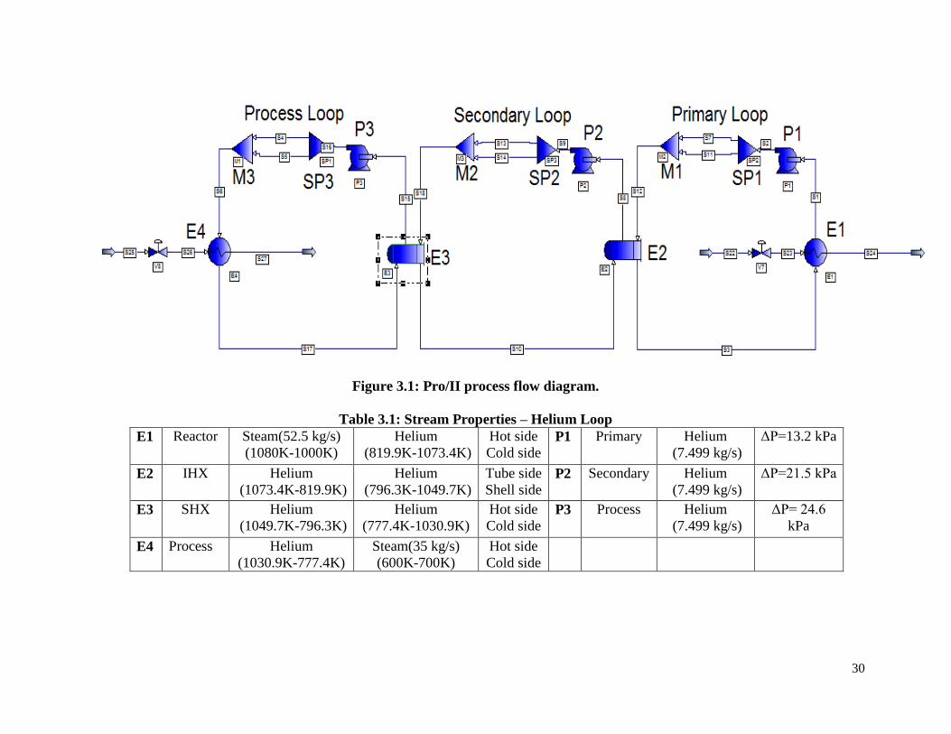
A Steady-State Model of the system was created in PRO/II 9.2. Figure 3.1 shows the process flow
diagram consisting of a primary loop carrying the heat from the reactor, the secondary loop which
receives the thermal energy from the primary loop in the intermediate heat exchanger, and the process
loop that receives the thermal energy from the secondary loop via the secondary heat exchanger. The
significant components in the system are as follows:
E1- This heat exchanger is used to model the effects of the nuclear reactor. All heat exchangers were
modeled for a 10MW design. This heat exchanger had a constant duty of 10MW.
29
E2: This is the IHX. Tube dimensions were taken from previous data for fluted tube. A heat transfer
area of 601.9 m2. The overall heat transfer coefficient used was 775 W/(m2*K).
E3: This is the SHX for the system. The heat transfer properties for an offset strip-fin heat exchanger
was used. The heat transfer area used was 212.6 m2. The overall heat transfer coefficient used was
2181 W/(m2*K).
E4: This heat exchanger was used to cool down helium to original inlet temperature in process loop.
A constant overall duty of 10MW was also used for the heat exchanger.
P(1-3): These are the pumps for each loop. They have a pressure rise across them equal to all of the
pressure drops across the heat exchangers in any given loop.
SP(1-3) and M(1-3): The SP and M units are splitter and mixers, respectively. These have no
functionality in PRO/II but are essential for the simulations by Dynsim.
Initially, helium was used as the heat transfer medium in all three loops to obtain dynamic
behavior for various disturbances in different loops. Similar simulations were subsequently also
conducted with both FLiNaK and FLiBe. The values of temperatures and flow rates for various
streams are shown in Table 3.1 for a system having a nominal duty of 10 MW.
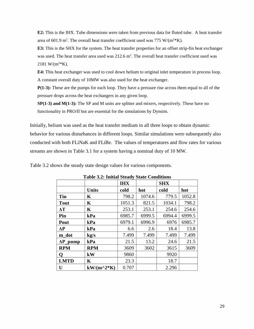
Table 3.2 shows the steady state design values for various components.
Table 3.2: Initial Steady State Conditions
IHX SHX
Units cold hot cold hot
Tin K 798.2 1074.6 779.5 1052.8
Tout K 1051.3 821.5 1034.1 798.2
ΔT K 253.1 253.1 254.6 254.6
Pin kPa 6985.7 6999.5 6994.4 6999.5
Pout kPa 6979.1 6996.9 6976 6985.7
ΔP kPa 6.6 2.6 18.4 13.8
m_dot kg/s 7.499 7.499 7.499 7.499
ΔP_pump kPa 21.5 13.2 24.6 21.5
RPM RPM 3609 3602 3615 3609
Q kW 9860 9920
LMTD K 23.3 18.7
U kW/(m^2*K) 0.707 2.296
30
Figure 3.1: Pro/II process flow diagram.
Table 3.1: Stream Properties – Helium Loop
E1 Reactor
Steam(52.5 kg/s)
(1080K-1000K)
Helium
(819.9K-1073.4K)
Hot side
Cold side P1 Primary Helium
(7.499 kg/s)
ΔP=13.2 kPa
E2 IHX
Helium
(1073.4K-819.9K)
Helium
(796.3K-1049.7K)
Tube side
Shell side P2 Secondary Helium
(7.499 kg/s)
ΔP=21.5 kPa
E3 SHX Helium
(1049.7K-796.3K)
Helium
(777.4K-1030.9K)
Hot side
Cold side P3 Process Helium
(7.499 kg/s)
ΔP= 24.6
kPa
E4 Process Helium
(1030.9K-777.4K)
Steam(35 kg/s)
(600K-700K)
Hot side
Cold side
31
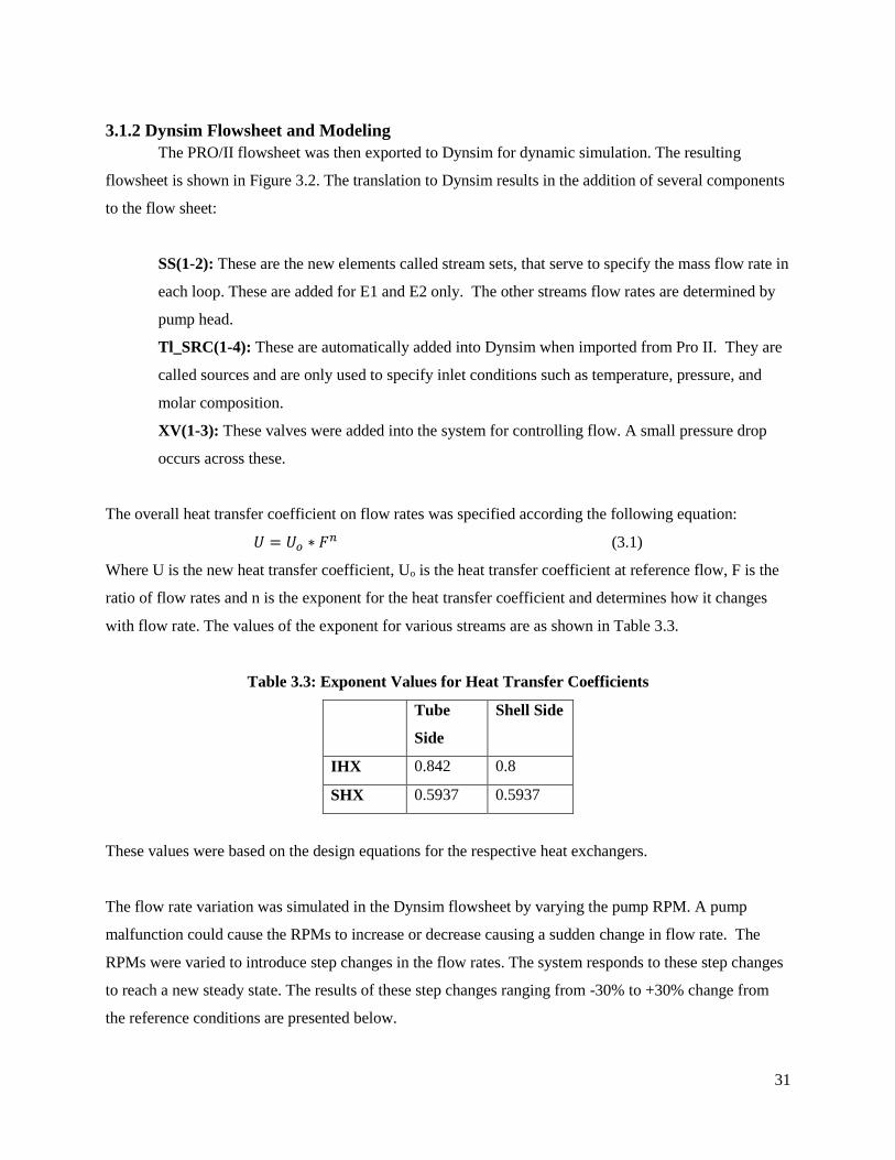
3.1.2 Dynsim Flowsheet and Modeling
The PRO/II flowsheet was then exported to Dynsim for dynamic simulation. The resulting
flowsheet is shown in Figure 3.2. The translation to Dynsim results in the addition of several components
to the flow sheet:
SS(1-2): These are the new elements called stream sets, that serve to specify the mass flow rate in
each loop. These are added for E1 and E2 only. The other streams flow rates are determined by
pump head.
Tl_SRC(1-4): These are automatically added into Dynsim when imported from Pro II. They are
called sources and are only used to specify inlet conditions such as temperature, pressure, and
molar composition.
XV(1-3): These valves were added into the system for controlling flow. A small pressure drop
occurs across these.
The overall heat transfer coefficient on flow rates was specified according the following equation:
𝑈 = 𝑈𝑜 ∗ 𝐹𝑛 (3.1)
Where U is the new heat transfer coefficient, Uo is the heat transfer coefficient at reference flow, F is the
ratio of flow rates and n is the exponent for the heat transfer coefficient and determines how it changes
with flow rate. The values of the exponent for various streams are as shown in Table 3.3.
Table 3.3: Exponent Values for Heat Transfer Coefficients
Tube
Side
Shell Side
IHX 0.842 0.8
SHX 0.5937 0.5937
These values were based on the design equations for the respective heat exchangers.
The flow rate variation was simulated in the Dynsim flowsheet by varying the pump RPM. A pump
malfunction could cause the RPMs to increase or decrease causing a sudden change in flow rate. The
RPMs were varied to introduce step changes in the flow rates. The system responds to these step changes
to reach a new steady state. The results of these step changes ranging from -30% to +30% change from
the reference conditions are presented below.
32
Figure 3.2: Process flow diagram of all helium process in Dynsim.
33
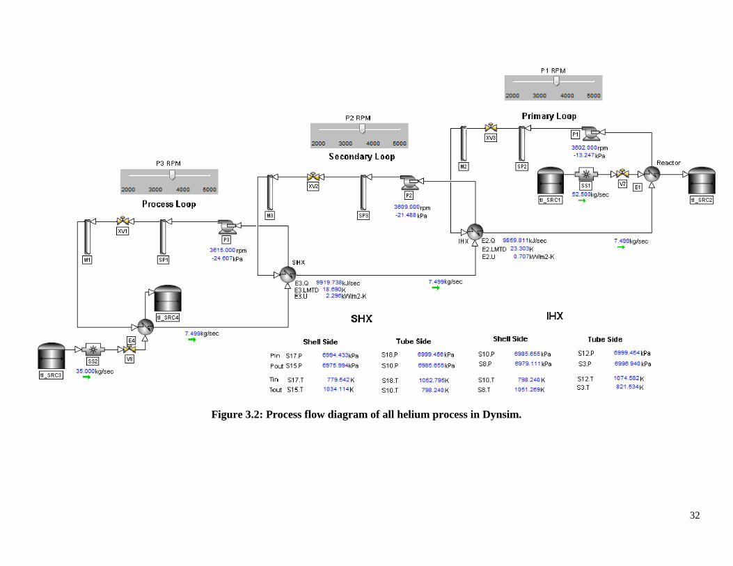
3.1.3 Simulation of System Behavior for Flow Rate Disturbances
Several different attributes were looked at after each step change. These include overall heat
transfer coefficient, log mean temperature difference, heat duty, temperature change, and the pressure
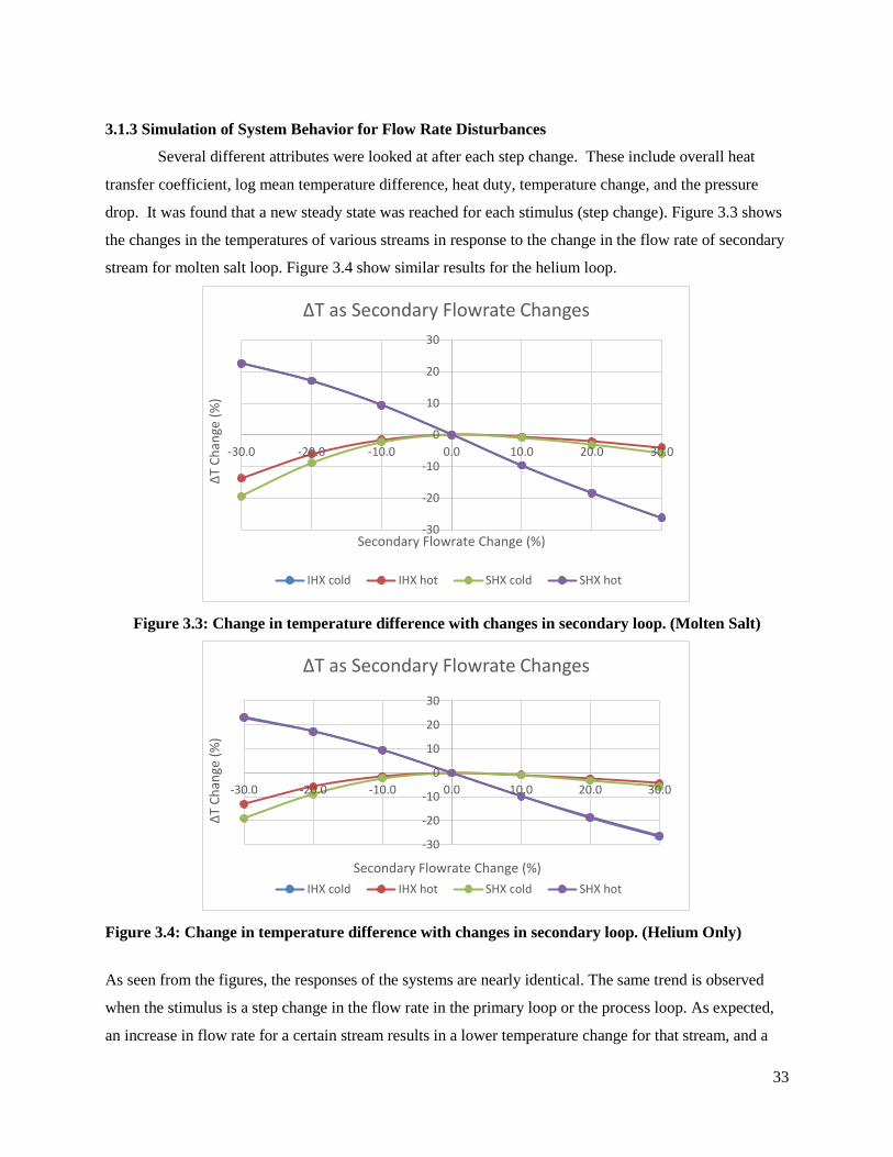
drop. It was found that a new steady state was reached for each stimulus (step change). Figure 3.3 shows
the changes in the temperatures of various streams in response to the change in the flow rate of secondary
stream for molten salt loop. Figure 3.4 show similar results for the helium loop.
Figure 3.3: Change in temperature difference with changes in secondary loop. (Molten Salt)
Figure 3.4: Change in temperature difference with changes in secondary loop. (Helium Only)
As seen from the figures, the responses of the systems are nearly identical. The same trend is observed
when the stimulus is a step change in the flow rate in the primary loop or the process loop. As expected,
an increase in flow rate for a certain stream results in a lower temperature change for that stream, and a
-30
-20
-10
0
10
20
30
-30.0 -20.0 -10.0 0.0 10.0 20.0 30.0
ΔT
Ch
ange
(%
)
Secondary Flowrate Change (%)
ΔT as Secondary Flowrate Changes
IHX cold IHX hot SHX cold SHX hot
-30
-20
-10
0
10
20
30
-30.0 -20.0 -10.0 0.0 10.0 20.0 30.0
ΔT
Ch
ange
(%
)
Secondary Flowrate Change (%)
ΔT as Secondary Flowrate Changes
IHX cold IHX hot SHX cold SHX hot
34
decrease in the flow rate will result in a higher temperature change. In most cases, the net heat transferred
(heat duty of the heat exchanger described later) decreases, and most streams a decrease in temperature is
observed as seen from the figures.
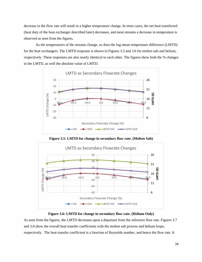
As the temperatures of the streams change, so does the log-mean temperature difference (LMTD)
for the heat exchangers. The LMTD response is shown in Figures 3.5 and 3.6 for molten salt and helium,
respectively. These responses are also nearly identical to each other. The figures show both the % changes
in the LMTD, as well the absolute value of LMTD.
Figure 3.5: LMTD for change in secondary flow rate. (Molten Salt)
Figure 3.6: LMTD for change in secondary flow rate. (Helium Only)
As seen from the figures, the LMTD decreases upon a departure from the reference flow rate. Figures 3.7
and 3.8 show the overall heat transfer coefficients with the molten salt process and helium loops,
respectively. The heat transfer coefficient is a function of Reynolds number, and hence the flow rate. It
6
11
16
21
26
-30
-20
-10
0
10
20
30
-30.0 -20.0 -10.0 0.0 10.0 20.0 30.0 LMTD
(K
)
LMTD
Ch
ange
(%
)
Secondary Flowrate Change (%)
LMTD as Secondary Flowrate Changes
IHX SHX LMTD IHX LMTD SHX
6
11
16
21
26
-30
-20
-10
0
10
20
30
-30.0 -20.0 -10.0 0.0 10.0 20.0 30.0 LMTD
(K
)
LMTD
Ch
ange
(%
)
Secondary Flowrate Change (%)
LMTD as Secondary Flowrate Changes
IHX SHX LMTD IHX LMTD SHX
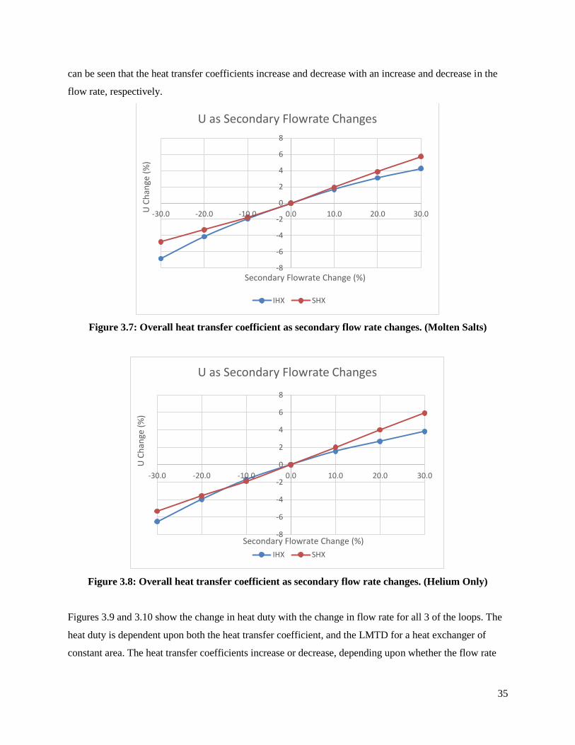
35
can be seen that the heat transfer coefficients increase and decrease with an increase and decrease in the
flow rate, respectively.
Figure 3.7: Overall heat transfer coefficient as secondary flow rate changes. (Molten Salts)
Figure 3.8: Overall heat transfer coefficient as secondary flow rate changes. (Helium Only)
Figures 3.9 and 3.10 show the change in heat duty with the change in flow rate for all 3 of the loops. The
heat duty is dependent upon both the heat transfer coefficient, and the LMTD for a heat exchanger of
constant area. The heat transfer coefficients increase or decrease, depending upon whether the flow rate
-8
-6
-4
-2
0
2
4
6
8
-30.0 -20.0 -10.0 0.0 10.0 20.0 30.0U C
han
ge (
%)
Secondary Flowrate Change (%)
U as Secondary Flowrate Changes
IHX SHX
-8
-6
-4
-2
0
2
4
6
8
-30.0 -20.0 -10.0 0.0 10.0 20.0 30.0
U C
han
ge (
%)
Secondary Flowrate Change (%)
U as Secondary Flowrate Changes
IHX SHX

36
has increased or decreased. In combination with the LMTD variation, this leads to a net decrease in the
heat duty in all cases, except for the case of increase in the primary flow rate.
Figure 3.9: Changes in duty with changes in the flow rate of each loop. (Molten Salt)
Figure 3.10: Changes in duty with changes in the flow rate of each loop. (Helium only)
It is also found that the flow rate change of a stream causes a change in flow rates of other streams. For
example, a change in the flow rate of the secondary loop causes a change in the flow rates in the process
and primary loops. This is due to the fact that the resultant temperature changes affect the stream
properties. The effect is complex and a quantitative description is not yet developed. The flow rate
changes are more pronounced for helium streams than the molten salt streams, as can be seen from figures
3.11 and 3.12.
-20
-15
-10
-5
0
5
-30.0 -20.0 -10.0 0.0 10.0 20.0 30.0
Du
ty C
han
ge (
%)
Flowrate Change (%)
Duty Change with Flowrate Change
Change in Process Flowrate Change in Secondary Flowrate
Change in Primary Flowrate
-20
-15
-10
-5
0
5
-30.0 -20.0 -10.0 0.0 10.0 20.0 30.0
Du
ty C
han
ge (
%)
Flowrate Change (%)
Change in Process Flowrate Change in Secondary Flowrate
Change in Primary Flowrate
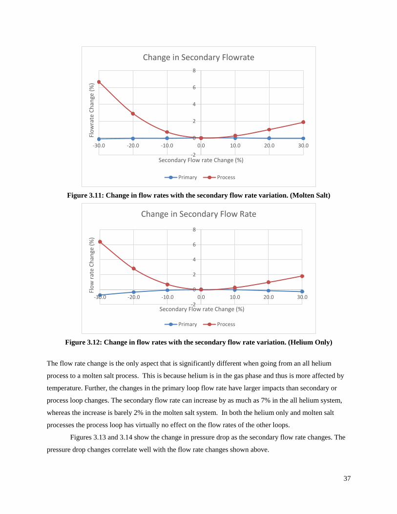
37
Figure 3.11: Change in flow rates with the secondary flow rate variation. (Molten Salt)
Figure 3.12: Change in flow rates with the secondary flow rate variation. (Helium Only)
The flow rate change is the only aspect that is significantly different when going from an all helium
process to a molten salt process. This is because helium is in the gas phase and thus is more affected by
temperature. Further, the changes in the primary loop flow rate have larger impacts than secondary or
process loop changes. The secondary flow rate can increase by as much as 7% in the all helium system,
whereas the increase is barely 2% in the molten salt system. In both the helium only and molten salt
processes the process loop has virtually no effect on the flow rates of the other loops.
Figures 3.13 and 3.14 show the change in pressure drop as the secondary flow rate changes. The
pressure drop changes correlate well with the flow rate changes shown above.
-2
0
2
4
6
8
-30.0 -20.0 -10.0 0.0 10.0 20.0 30.0
Flo
wra
te C
han
ge (
%)
Secondary Flow rate Change (%)
Change in Secondary Flowrate
Primary Process
-2
0
2
4
6
8
-30.0 -20.0 -10.0 0.0 10.0 20.0 30.0
Flo
w r
ate
Ch
ange
(%
)
Secondary Flow rate Change (%)
Change in Secondary Flow Rate
Primary Process
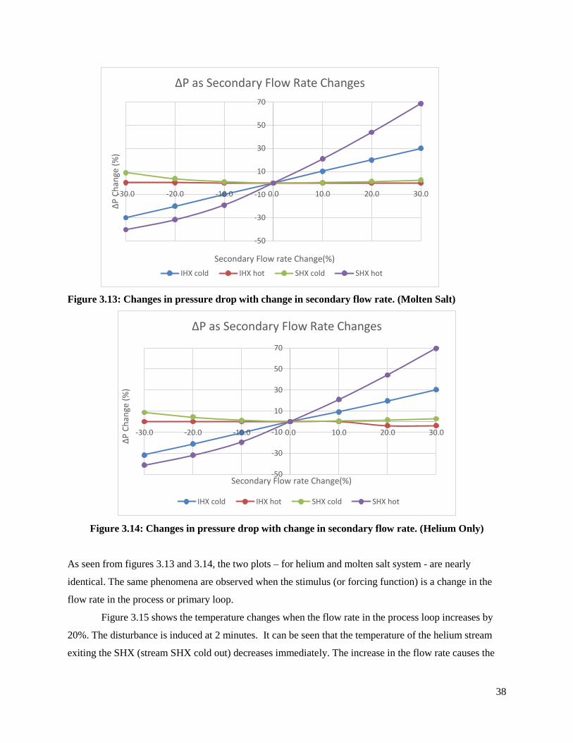
38
Figure 3.13: Changes in pressure drop with change in secondary flow rate. (Molten Salt)
Figure 3.14: Changes in pressure drop with change in secondary flow rate. (Helium Only)
As seen from figures 3.13 and 3.14, the two plots – for helium and molten salt system - are nearly
identical. The same phenomena are observed when the stimulus (or forcing function) is a change in the
flow rate in the process or primary loop.
Figure 3.15 shows the temperature changes when the flow rate in the process loop increases by
20%. The disturbance is induced at 2 minutes. It can be seen that the temperature of the helium stream
exiting the SHX (stream SHX cold out) decreases immediately. The increase in the flow rate causes the
-50
-30
-10
10
30
50
70
-30.0 -20.0 -10.0 0.0 10.0 20.0 30.0
ΔP
Ch
ange
(%
)
Secondary Flow rate Change(%)
ΔP as Secondary Flow Rate Changes
IHX cold IHX hot SHX cold SHX hot
-50
-30
-10
10
30
50
70
-30.0 -20.0 -10.0 0.0 10.0 20.0 30.0
ΔP
Ch
ange
(%
)
Secondary Flow rate Change(%)
ΔP as Secondary Flow Rate Changes
IHX cold IHX hot SHX cold SHX hot
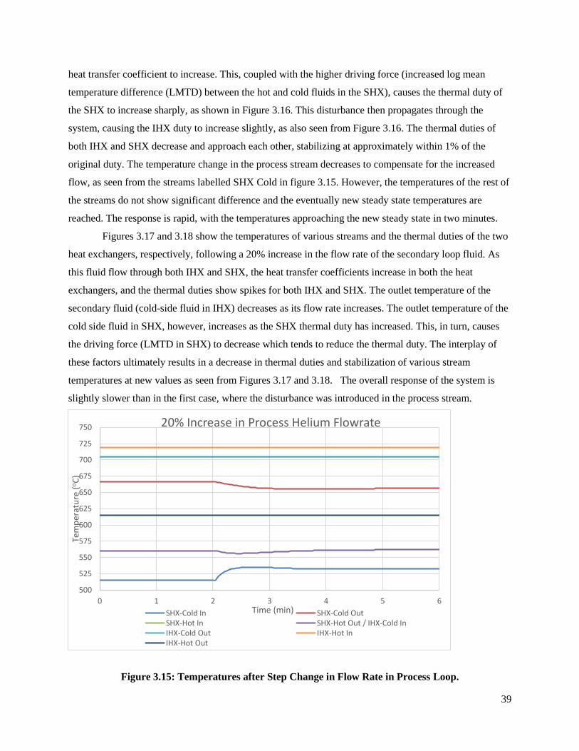
39
heat transfer coefficient to increase. This, coupled with the higher driving force (increased log mean
temperature difference (LMTD) between the hot and cold fluids in the SHX), causes the thermal duty of
the SHX to increase sharply, as shown in Figure 3.16. This disturbance then propagates through the
system, causing the IHX duty to increase slightly, as also seen from Figure 3.16. The thermal duties of
both IHX and SHX decrease and approach each other, stabilizing at approximately within 1% of the
original duty. The temperature change in the process stream decreases to compensate for the increased
flow, as seen from the streams labelled SHX Cold in figure 3.15. However, the temperatures of the rest of
the streams do not show significant difference and the eventually new steady state temperatures are
reached. The response is rapid, with the temperatures approaching the new steady state in two minutes.
Figures 3.17 and 3.18 show the temperatures of various streams and the thermal duties of the two
heat exchangers, respectively, following a 20% increase in the flow rate of the secondary loop fluid. As
this fluid flow through both IHX and SHX, the heat transfer coefficients increase in both the heat
exchangers, and the thermal duties show spikes for both IHX and SHX. The outlet temperature of the
secondary fluid (cold-side fluid in IHX) decreases as its flow rate increases. The outlet temperature of the
cold side fluid in SHX, however, increases as the SHX thermal duty has increased. This, in turn, causes
the driving force (LMTD in SHX) to decrease which tends to reduce the thermal duty. The interplay of
these factors ultimately results in a decrease in thermal duties and stabilization of various stream
temperatures at new values as seen from Figures 3.17 and 3.18. The overall response of the system is
slightly slower than in the first case, where the disturbance was introduced in the process stream.
Figure 3.15: Temperatures after Step Change in Flow Rate in Process Loop.
500
525
550
575
600
625
650
675
700
725
750
0 1 2 3 4 5 6
Tem
per
atu
re (
oC
)
Time (min)
20% Increase in Process Helium Flowrate
SHX-Cold In SHX-Cold OutSHX-Hot In SHX-Hot Out / IHX-Cold InIHX-Cold Out IHX-Hot InIHX-Hot Out
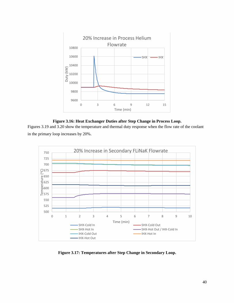
40
Figure 3.16: Heat Exchanger Duties after Step Change in Process Loop.
Figures 3.19 and 3.20 show the temperature and thermal duty response when the flow rate of the coolant
in the primary loop increases by 20%.
Figure 3.17: Temperatures after Step Change in Secondary Loop.
9600
9800
10000
10200
10400
10600
10800
0 3 6 9 12 15
Du
ty (
kW)
Time (min)
20% Increase in Process Helium Flowrate
SHX IHX
500
525
550
575
600
625
650
675
700
725
750
0 1 2 3 4 5 6 7 8 9 10
Tem
per
atu
re (
oC
)
Time (min)
20% Increase in Secondary FLiNaK Flowrate
SHX-Cold In SHX-Cold Out
SHX-Hot In SHX-Hot Out / IHX-Cold In
IHX-Cold Out IHX-Hot In
IHX-Hot Out
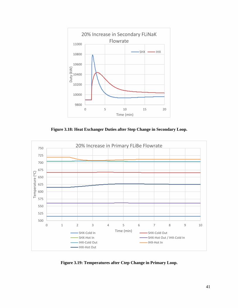
41
Figure 3.18: Heat Exchanger Duties after Step Change in Secondary Loop.
Figure 3.19: Temperatures after Ctep Change in Primary Loop.
9800
10000
10200
10400
10600
10800
11000
0 5 10 15 20
Du
ty (
kW)
Time (min)
20% Increase in Secondary FLiNaK Flowrate
SHX IHX
500
525
550
575
600
625
650
675
700
725
750
0 1 2 3 4 5 6 7 8 9 10
Tem
per
atu
re (
oC
)
Time (min)
20% Increase in Primary FLiBe Flowrate
SHX-Cold In SHX-Cold Out
SHX-Hot In SHX-Hot Out / IHX-Cold In
IHX-Cold Out IHX-Hot In
IHX-Hot Out
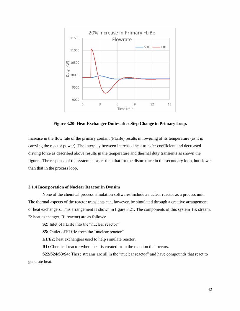
42
Figure 3.20: Heat Exchanger Duties after Step Change in Primary Loop.
Increase in the flow rate of the primary coolant (FLiBe) results in lowering of its temperature (as it is
carrying the reactor power). The interplay between increased heat transfer coefficient and decreased
driving force as described above results in the temperature and thermal duty transients as shown the
figures. The response of the system is faster than that for the disturbance in the secondary loop, but slower
than that in the process loop.
3.1.4 Incorporation of Nuclear Reactor in Dynsim
None of the chemical process simulation softwares include a nuclear reactor as a process unit.
The thermal aspects of the reactor transients can, however, be simulated through a creative arrangement
of heat exchangers. This arrangement is shown in figure 3.21. The components of this system (S: stream,
E: heat exchanger, R: reactor) are as follows:
S2: Inlet of FLiBe into the “nuclear reactor”
S5: Outlet of FLiBe from the “nuclear reactor”
E1/E2: heat exchangers used to help simulate reactor.
R1: Chemical reactor where heat is created from the reaction that occurs.
S22/S24/S3/S4: These streams are all in the “nuclear reactor” and have compounds that react to
generate heat.
9000
9500
10000
10500
11000
11500
0 3 6 9 12 15
Du
ty (
kW)
Time (min)
20% Increase in Primary FLiBe Flowrate
SHX IHX
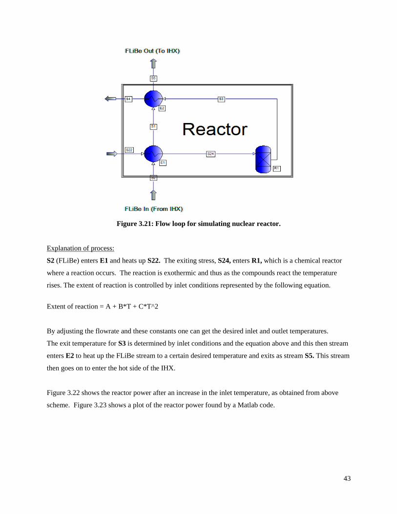
43
Figure 3.21: Flow loop for simulating nuclear reactor.
Explanation of process:
S2 (FLiBe) enters E1 and heats up S22. The exiting stress, S24, enters R1, which is a chemical reactor
where a reaction occurs. The reaction is exothermic and thus as the compounds react the temperature
rises. The extent of reaction is controlled by inlet conditions represented by the following equation.
Extent of reaction = A + B*T + C*T^2
By adjusting the flowrate and these constants one can get the desired inlet and outlet temperatures.
The exit temperature for S3 is determined by inlet conditions and the equation above and this then stream
enters E2 to heat up the FLiBe stream to a certain desired temperature and exits as stream S5. This stream
then goes on to enter the hot side of the IHX.
Figure 3.22 shows the reactor power after an increase in the inlet temperature, as obtained from above
scheme. Figure 3.23 shows a plot of the reactor power found by a Matlab code.
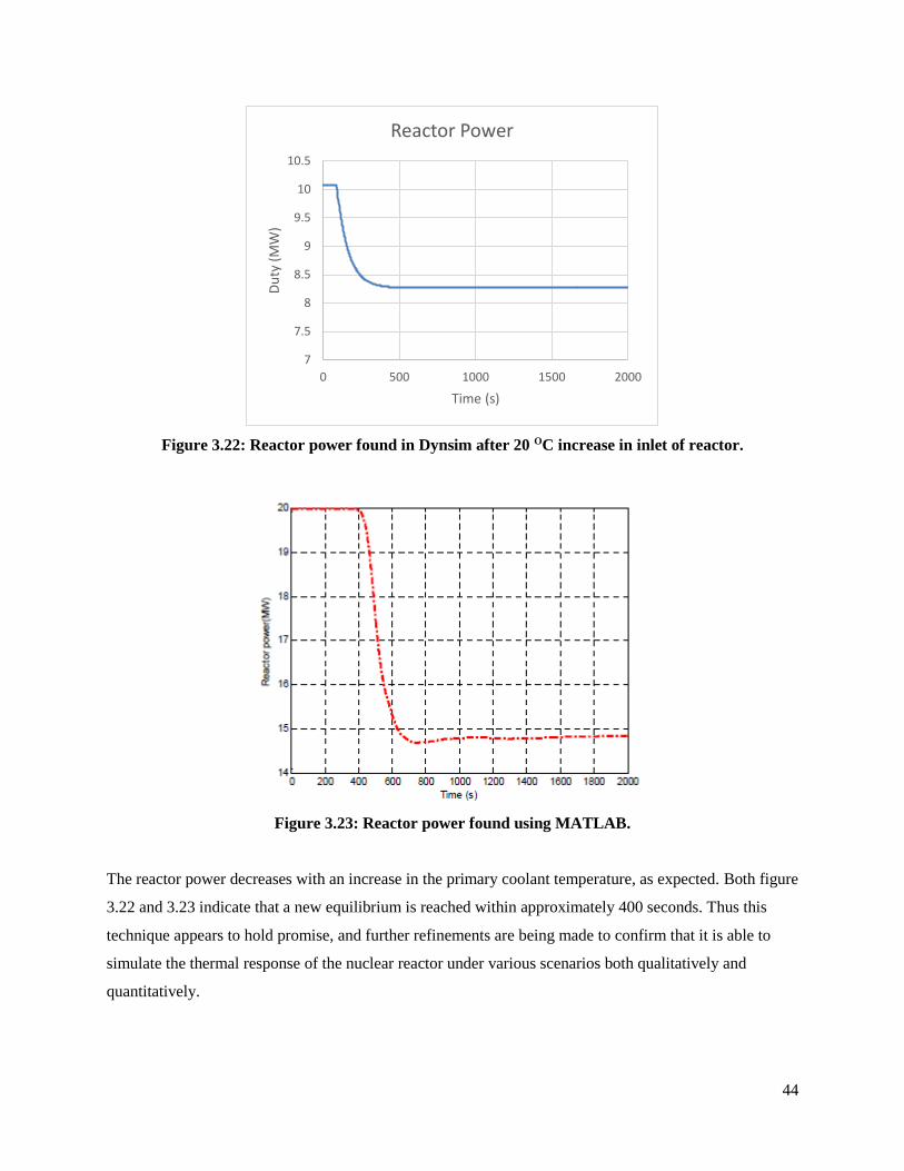
44
Figure 3.22: Reactor power found in Dynsim after 20 OC increase in inlet of reactor.
Figure 3.23: Reactor power found using MATLAB.
The reactor power decreases with an increase in the primary coolant temperature, as expected. Both figure
3.22 and 3.23 indicate that a new equilibrium is reached within approximately 400 seconds. Thus this
technique appears to hold promise, and further refinements are being made to confirm that it is able to
simulate the thermal response of the nuclear reactor under various scenarios both qualitatively and
quantitatively.
7
7.5
8
8.5
9
9.5
10
10.5
0 500 1000 1500 2000
Du
ty (
MW
)
Time (s)
Reactor Power
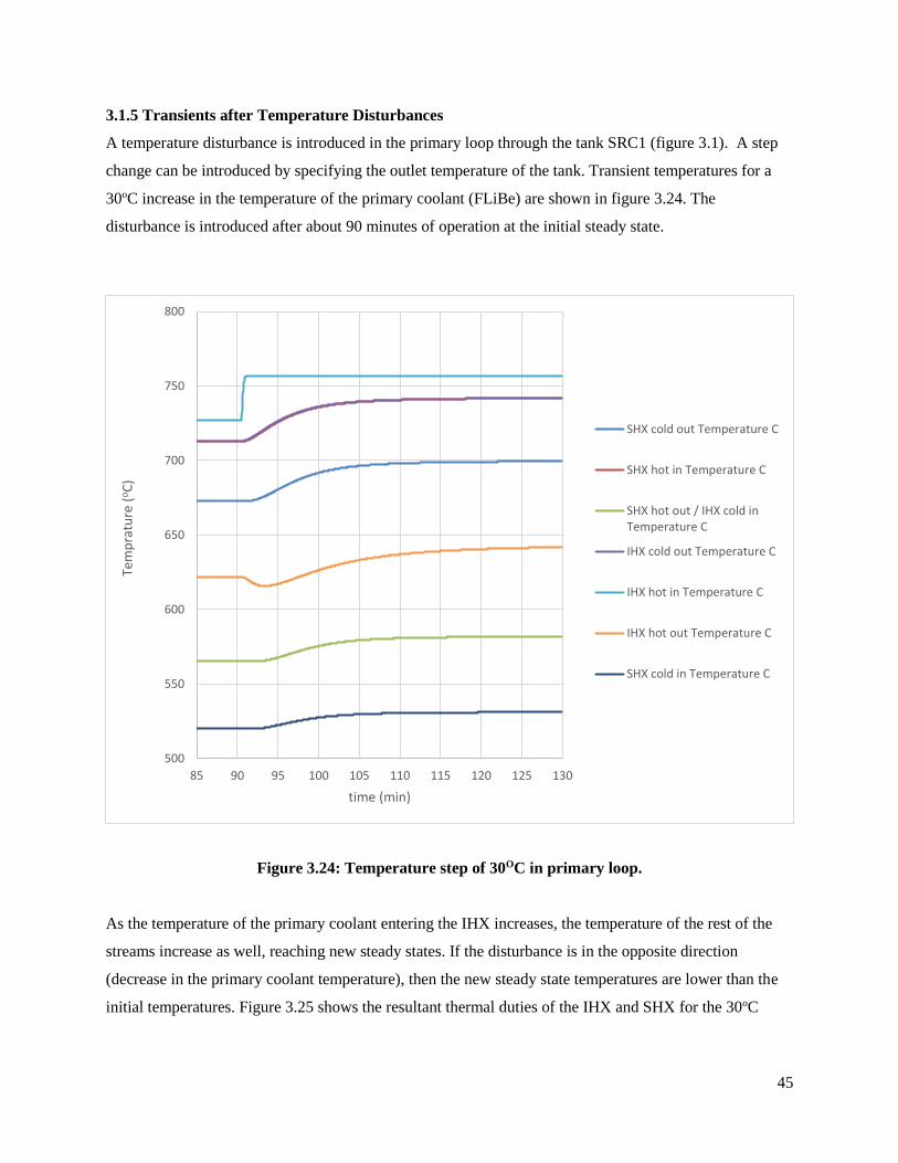
45
3.1.5 Transients after Temperature Disturbances
A temperature disturbance is introduced in the primary loop through the tank SRC1 (figure 3.1). A step
change can be introduced by specifying the outlet temperature of the tank. Transient temperatures for a
30oC increase in the temperature of the primary coolant (FLiBe) are shown in figure 3.24. The
disturbance is introduced after about 90 minutes of operation at the initial steady state.
Figure 3.24: Temperature step of 30OC in primary loop.
As the temperature of the primary coolant entering the IHX increases, the temperature of the rest of the
streams increase as well, reaching new steady states. If the disturbance is in the opposite direction
(decrease in the primary coolant temperature), then the new steady state temperatures are lower than the
initial temperatures. Figure 3.25 shows the resultant thermal duties of the IHX and SHX for the 30oC
500
550
600
650
700
750
800
85 90 95 100 105 110 115 120 125 130
Tem
pra
ture
(oC
)
time (min)
SHX cold out Temperature C
SHX hot in Temperature C
SHX hot out / IHX cold inTemperature C
IHX cold out Temperature C
IHX hot in Temperature C
IHX hot out Temperature C
SHX cold in Temperature C
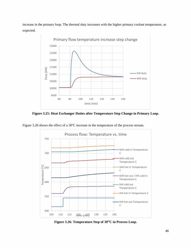
46
increase in the primary loop. The thermal duty increases with the higher primary coolant temperature, as
expected.
Figure 3.25: Heat Exchanger Duties after Temperature Step Change in Primary Loop.
Figure 3.26 shows the effect of a 30oC increase in the temperature of the process stream.
Figure 3.26: Temperature Step of 30OC in Process Loop.
9500
10000
10500
11000
11500
12000
12500
13000
80 90 100 110 120 130 140
Du
ty (
kW)
time (min)
Primary flow temperature increase step change
IHX duty
SHX duty
500
550
600
650
700
750
105 110 115 120 125 130 135 140
Tem
pra
ture
(oC
)
time (min)
Process flow: Temperature vs. time
SHX cold in TemperatureC
SHX cold outTemperature C
SHX hot in TemperatureC
SHX hot out / IHX cold inTemperature C
IHX cold outTemperature C
IHX hot in Temperature C
IHX hot out TemperatureC
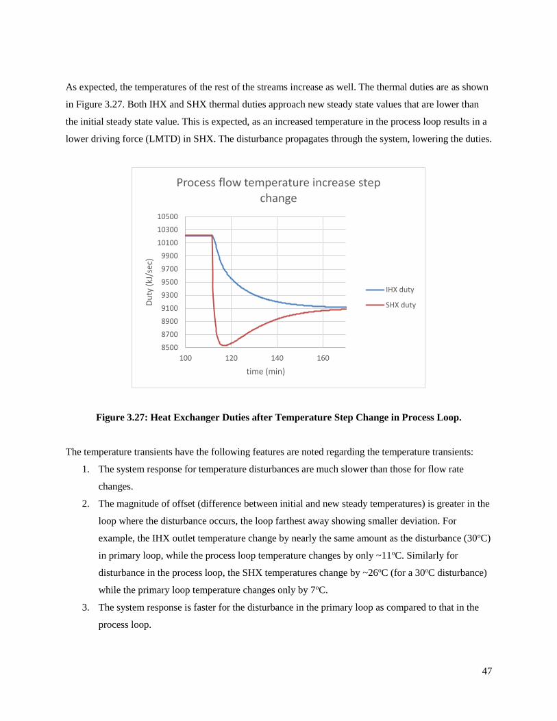
47
As expected, the temperatures of the rest of the streams increase as well. The thermal duties are as shown
in Figure 3.27. Both IHX and SHX thermal duties approach new steady state values that are lower than
the initial steady state value. This is expected, as an increased temperature in the process loop results in a
lower driving force (LMTD) in SHX. The disturbance propagates through the system, lowering the duties.
Figure 3.27: Heat Exchanger Duties after Temperature Step Change in Process Loop.
The temperature transients have the following features are noted regarding the temperature transients:
1. The system response for temperature disturbances are much slower than those for flow rate
changes.
2. The magnitude of offset (difference between initial and new steady temperatures) is greater in the
loop where the disturbance occurs, the loop farthest away showing smaller deviation. For
example, the IHX outlet temperature change by nearly the same amount as the disturbance (30oC)
in primary loop, while the process loop temperature changes by only ~11oC. Similarly for
disturbance in the process loop, the SHX temperatures change by ~26oC (for a 30oC disturbance)
while the primary loop temperature changes only by 7oC.
3. The system response is faster for the disturbance in the primary loop as compared to that in the
process loop.
8500
8700
8900
9100
9300
9500
9700
9900
10100
10300
10500
100 120 140 160
Du
ty (
kJ/s
ec)
time (min)
Process flow temperature increase step change
IHX duty
SHX duty
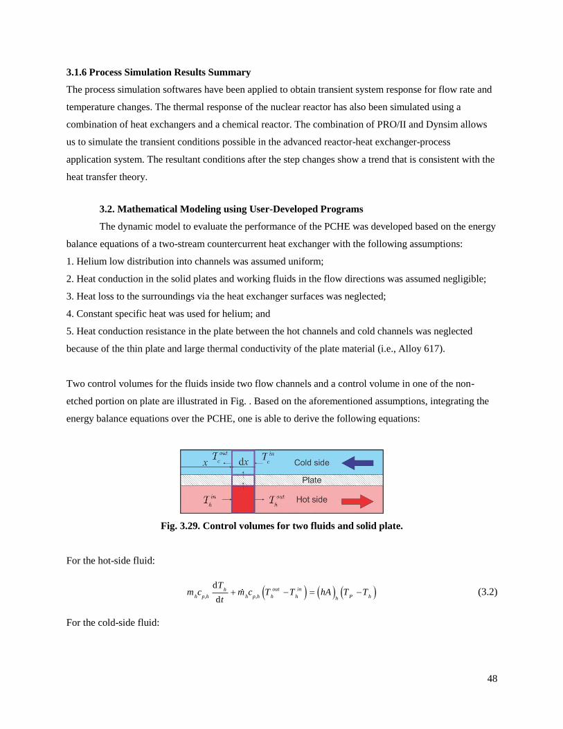
48
3.1.6 Process Simulation Results Summary
The process simulation softwares have been applied to obtain transient system response for flow rate and
temperature changes. The thermal response of the nuclear reactor has also been simulated using a
combination of heat exchangers and a chemical reactor. The combination of PRO/II and Dynsim allows
us to simulate the transient conditions possible in the advanced reactor-heat exchanger-process
application system. The resultant conditions after the step changes show a trend that is consistent with the
heat transfer theory.
3.2. Mathematical Modeling using User-Developed Programs
The dynamic model to evaluate the performance of the PCHE was developed based on the energy
balance equations of a two-stream countercurrent heat exchanger with the following assumptions:
1. Helium low distribution into channels was assumed uniform;
2. Heat conduction in the solid plates and working fluids in the flow directions was assumed negligible;
3. Heat loss to the surroundings via the heat exchanger surfaces was neglected;
4. Constant specific heat was used for helium; and
5. Heat conduction resistance in the plate between the hot channels and cold channels was neglected
because of the thin plate and large thermal conductivity of the plate material (i.e., Alloy 617).
Two control volumes for the fluids inside two flow channels and a control volume in one of the non-
etched portion on plate are illustrated in Fig. . Based on the aforementioned assumptions, integrating the
energy balance equations over the PCHE, one is able to derive the following equations:
Fig. 3.29. Control volumes for two fluids and solid plate.
For the hot-side fluid:
, ,
d
d
out inh
h p h h p h h h P hh
Tm c m c T T hA T T
t (3.2)
For the cold-side fluid:
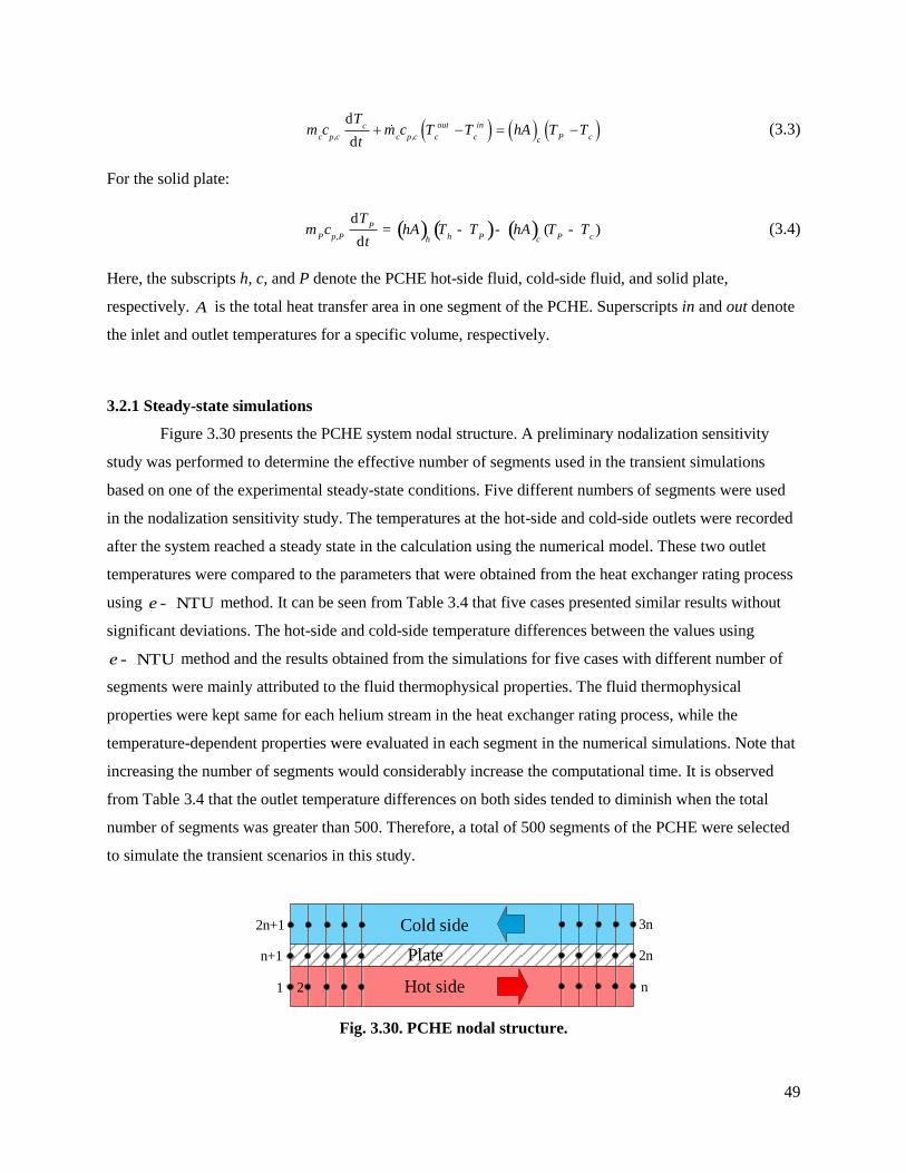
49
, ,
d
d
out inc
c p c c p c c c P cc
Tm c m c T T hA T T
t (3.3)
For the solid plate:
( ) ( ) ( ),
d( )
d
P
P p P h P P ch c
Tm c hA T T hA T T
t= - - - (3.4)
Here, the subscripts h, c, and P denote the PCHE hot-side fluid, cold-side fluid, and solid plate,
respectively. A is the total heat transfer area in one segment of the PCHE. Superscripts in and out denote
the inlet and outlet temperatures for a specific volume, respectively.
3.2.1 Steady-state simulations
Figure 3.30 presents the PCHE system nodal structure. A preliminary nodalization sensitivity
study was performed to determine the effective number of segments used in the transient simulations
based on one of the experimental steady-state conditions. Five different numbers of segments were used
in the nodalization sensitivity study. The temperatures at the hot-side and cold-side outlets were recorded
after the system reached a steady state in the calculation using the numerical model. These two outlet
temperatures were compared to the parameters that were obtained from the heat exchanger rating process
using NTUe - method. It can be seen from Table 3.4 that five cases presented similar results without
significant deviations. The hot-side and cold-side temperature differences between the values using
NTUe - method and the results obtained from the simulations for five cases with different number of
segments were mainly attributed to the fluid thermophysical properties. The fluid thermophysical
properties were kept same for each helium stream in the heat exchanger rating process, while the
temperature-dependent properties were evaluated in each segment in the numerical simulations. Note that
increasing the number of segments would considerably increase the computational time. It is observed
from Table 3.4 that the outlet temperature differences on both sides tended to diminish when the total
number of segments was greater than 500. Therefore, a total of 500 segments of the PCHE were selected
to simulate the transient scenarios in this study.
Fig. 3.30. PCHE nodal structure.
Cold side
Plate
Hot side1 2 n
3n
n+1
2n+1
2n
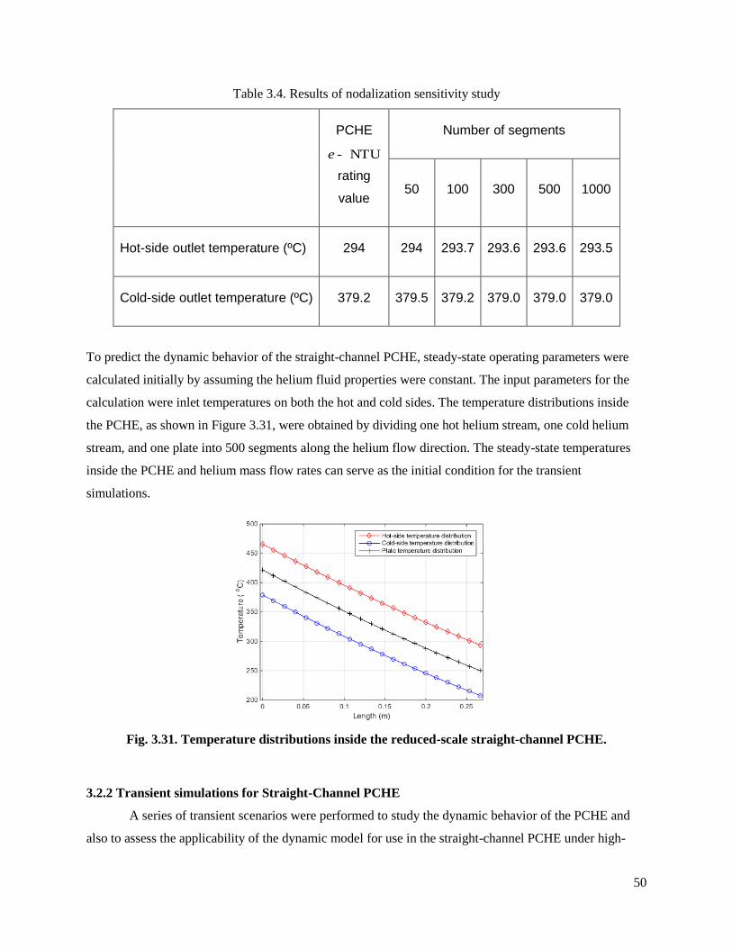
50
Table 3.4. Results of nodalization sensitivity study
PCHE
NTUe -
rating
value
Number of segments
50 100 300 500 1000
Hot-side outlet temperature (ºC) 294 294 293.7 293.6 293.6 293.5
Cold-side outlet temperature (ºC) 379.2 379.5 379.2 379.0 379.0 379.0
To predict the dynamic behavior of the straight-channel PCHE, steady-state operating parameters were
calculated initially by assuming the helium fluid properties were constant. The input parameters for the
calculation were inlet temperatures on both the hot and cold sides. The temperature distributions inside
the PCHE, as shown in Figure 3.31, were obtained by dividing one hot helium stream, one cold helium
stream, and one plate into 500 segments along the helium flow direction. The steady-state temperatures
inside the PCHE and helium mass flow rates can serve as the initial condition for the transient
simulations.
Fig. 3.31. Temperature distributions inside the reduced-scale straight-channel PCHE.
3.2.2 Transient simulations for Straight-Channel PCHE
A series of transient scenarios were performed to study the dynamic behavior of the PCHE and
also to assess the applicability of the dynamic model for use in the straight-channel PCHE under high-
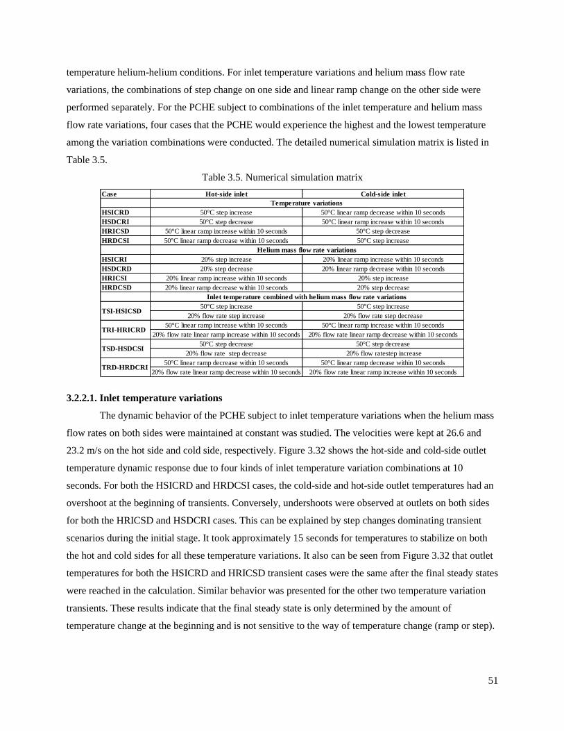
51
temperature helium-helium conditions. For inlet temperature variations and helium mass flow rate
variations, the combinations of step change on one side and linear ramp change on the other side were
performed separately. For the PCHE subject to combinations of the inlet temperature and helium mass
flow rate variations, four cases that the PCHE would experience the highest and the lowest temperature
among the variation combinations were conducted. The detailed numerical simulation matrix is listed in
Table 3.5.
Table 3.5. Numerical simulation matrix
3.2.2.1. Inlet temperature variations
The dynamic behavior of the PCHE subject to inlet temperature variations when the helium mass
flow rates on both sides were maintained at constant was studied. The velocities were kept at 26.6 and
23.2 m/s on the hot side and cold side, respectively. Figure 3.32 shows the hot-side and cold-side outlet
temperature dynamic response due to four kinds of inlet temperature variation combinations at 10
seconds. For both the HSICRD and HRDCSI cases, the cold-side and hot-side outlet temperatures had an
overshoot at the beginning of transients. Conversely, undershoots were observed at outlets on both sides
for both the HRICSD and HSDCRI cases. This can be explained by step changes dominating transient
scenarios during the initial stage. It took approximately 15 seconds for temperatures to stabilize on both
the hot and cold sides for all these temperature variations. It also can be seen from Figure 3.32 that outlet
temperatures for both the HSICRD and HRICSD transient cases were the same after the final steady states
were reached in the calculation. Similar behavior was presented for the other two temperature variation
transients. These results indicate that the final steady state is only determined by the amount of
temperature change at the beginning and is not sensitive to the way of temperature change (ramp or step).
Case Hot-side inlet Cold-side inlet
HSICRD 50°C step increase 50°C linear ramp decrease within 10 seconds
HSDCRI 50°C step decrease 50°C linear ramp increase within 10 seconds
HRICSD 50°C linear ramp increase within 10 seconds 50°C step decrease
HRDCSI 50°C linear ramp decrease within 10 seconds 50°C step increase
HSICRI 20% step increase 20% linear ramp increase within 10 seconds
HSDCRD 20% step decrease 20% linear ramp decrease within 10 seconds
HRICSI 20% linear ramp increase within 10 seconds 20% step increase
HRDCSD 20% linear ramp decrease within 10 seconds 20% step decrease
50°C step increase 50°C step increase
20% flow rate step increase 20% flow rate step decrease
50°C linear ramp increase within 10 seconds 50°C linear ramp increase within 10 seconds
20% flow rate linear ramp increase within 10 seconds 20% flow rate linear ramp decrease within 10 seconds
50°C step decrease 50°C step decrease
20% flow rate step decrease 20% flow ratestep increase
50°C linear ramp decrease within 10 seconds 50°C linear ramp decrease within 10 seconds
20% flow rate linear ramp decrease within 10 seconds 20% flow rate linear ramp increase within 10 secondsTRD-HRDCRI
Helium mass flow rate variations
Inlet temperature combined with helium mass flow rate variations
TSI-HSICSD
TRI-HRICRD
TSD-HSDCSI
Temperature variations
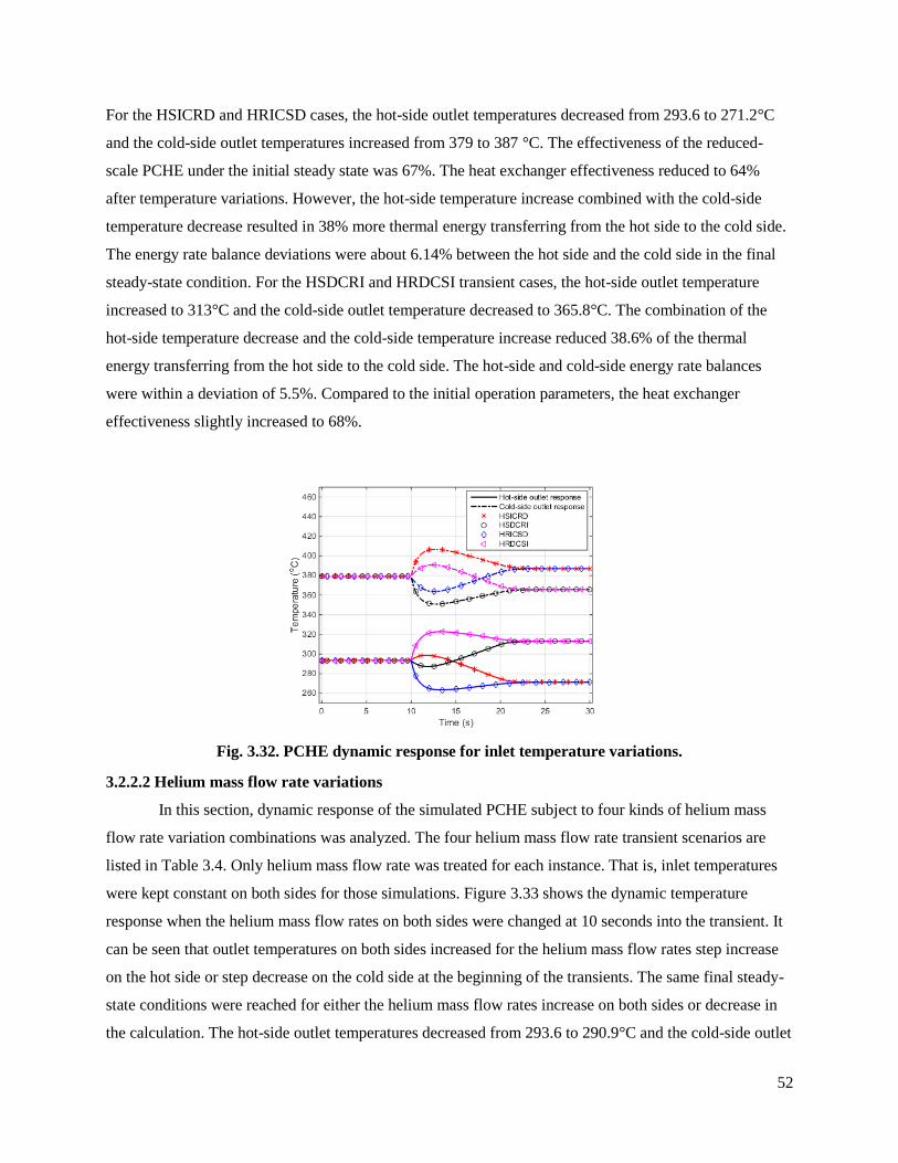
52
For the HSICRD and HRICSD cases, the hot-side outlet temperatures decreased from 293.6 to 271.2°C
and the cold-side outlet temperatures increased from 379 to 387 °C. The effectiveness of the reduced-
scale PCHE under the initial steady state was 67%. The heat exchanger effectiveness reduced to 64%
after temperature variations. However, the hot-side temperature increase combined with the cold-side
temperature decrease resulted in 38% more thermal energy transferring from the hot side to the cold side.
The energy rate balance deviations were about 6.14% between the hot side and the cold side in the final
steady-state condition. For the HSDCRI and HRDCSI transient cases, the hot-side outlet temperature
increased to 313°C and the cold-side outlet temperature decreased to 365.8°C. The combination of the
hot-side temperature decrease and the cold-side temperature increase reduced 38.6% of the thermal
energy transferring from the hot side to the cold side. The hot-side and cold-side energy rate balances
were within a deviation of 5.5%. Compared to the initial operation parameters, the heat exchanger
effectiveness slightly increased to 68%.
Fig. 3.32. PCHE dynamic response for inlet temperature variations.
3.2.2.2 Helium mass flow rate variations
In this section, dynamic response of the simulated PCHE subject to four kinds of helium mass
flow rate variation combinations was analyzed. The four helium mass flow rate transient scenarios are
listed in Table 3.4. Only helium mass flow rate was treated for each instance. That is, inlet temperatures
were kept constant on both sides for those simulations. Figure 3.33 shows the dynamic temperature
response when the helium mass flow rates on both sides were changed at 10 seconds into the transient. It
can be seen that outlet temperatures on both sides increased for the helium mass flow rates step increase
on the hot side or step decrease on the cold side at the beginning of the transients. The same final steady-
state conditions were reached for either the helium mass flow rates increase on both sides or decrease in
the calculation. The hot-side outlet temperatures decreased from 293.6 to 290.9°C and the cold-side outlet
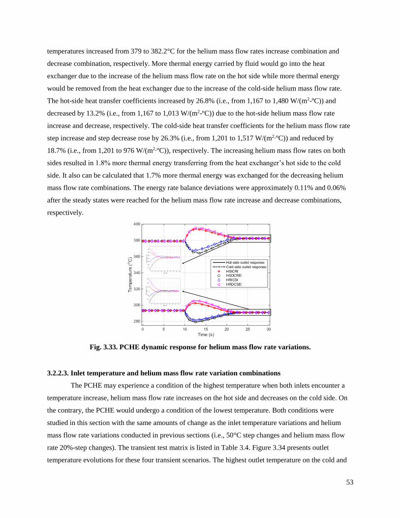
53
temperatures increased from 379 to 382.2°C for the helium mass flow rates increase combination and
decrease combination, respectively. More thermal energy carried by fluid would go into the heat
exchanger due to the increase of the helium mass flow rate on the hot side while more thermal energy
would be removed from the heat exchanger due to the increase of the cold-side helium mass flow rate.
The hot-side heat transfer coefficients increased by 26.8% (i.e., from 1,167 to 1,480 W/(m2-ºC)) and
decreased by 13.2% (i.e., from 1,167 to 1,013 W/(m2-ºC)) due to the hot-side helium mass flow rate
increase and decrease, respectively. The cold-side heat transfer coefficients for the helium mass flow rate
step increase and step decrease rose by 26.3% (i.e., from 1,201 to 1,517 W/(m2∙ºC)) and reduced by
18.7% (i.e., from 1,201 to 976 W/(m2∙ºC)), respectively. The increasing helium mass flow rates on both
sides resulted in 1.8% more thermal energy transferring from the heat exchanger’s hot side to the cold
side. It also can be calculated that 1.7% more thermal energy was exchanged for the decreasing helium
mass flow rate combinations. The energy rate balance deviations were approximately 0.11% and 0.06%
after the steady states were reached for the helium mass flow rate increase and decrease combinations,
respectively.
Fig. 3.33. PCHE dynamic response for helium mass flow rate variations.
3.2.2.3. Inlet temperature and helium mass flow rate variation combinations
The PCHE may experience a condition of the highest temperature when both inlets encounter a
temperature increase, helium mass flow rate increases on the hot side and decreases on the cold side. On
the contrary, the PCHE would undergo a condition of the lowest temperature. Both conditions were
studied in this section with the same amounts of change as the inlet temperature variations and helium
mass flow rate variations conducted in previous sections (i.e., 50°C step changes and helium mass flow
rate 20%-step changes). The transient test matrix is listed in Table 3.4. Figure 3.34 presents outlet
temperature evolutions for these four transient scenarios. The highest outlet temperature on the cold and
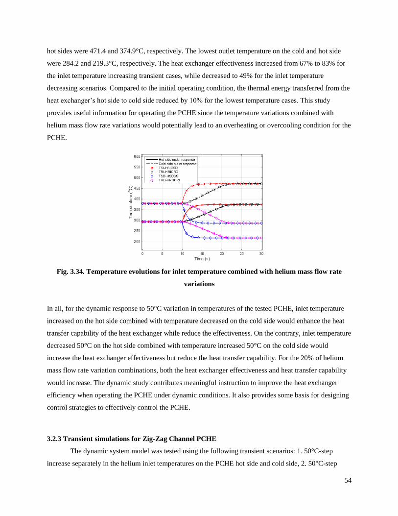
54
hot sides were 471.4 and 374.9°C, respectively. The lowest outlet temperature on the cold and hot side
were 284.2 and 219.3°C, respectively. The heat exchanger effectiveness increased from 67% to 83% for
the inlet temperature increasing transient cases, while decreased to 49% for the inlet temperature
decreasing scenarios. Compared to the initial operating condition, the thermal energy transferred from the
heat exchanger’s hot side to cold side reduced by 10% for the lowest temperature cases. This study
provides useful information for operating the PCHE since the temperature variations combined with
helium mass flow rate variations would potentially lead to an overheating or overcooling condition for the
PCHE.
Fig. 3.34. Temperature evolutions for inlet temperature combined with helium mass flow rate
variations
In all, for the dynamic response to 50°C variation in temperatures of the tested PCHE, inlet temperature
increased on the hot side combined with temperature decreased on the cold side would enhance the heat
transfer capability of the heat exchanger while reduce the effectiveness. On the contrary, inlet temperature
decreased 50°C on the hot side combined with temperature increased 50°C on the cold side would
increase the heat exchanger effectiveness but reduce the heat transfer capability. For the 20% of helium
mass flow rate variation combinations, both the heat exchanger effectiveness and heat transfer capability
would increase. The dynamic study contributes meaningful instruction to improve the heat exchanger
efficiency when operating the PCHE under dynamic conditions. It also provides some basis for designing
control strategies to effectively control the PCHE.
3.2.3 Transient simulations for Zig-Zag Channel PCHE
The dynamic system model was tested using the following transient scenarios: 1. 50°C-step
increase separately in the helium inlet temperatures on the PCHE hot side and cold side, 2. 50°C-step
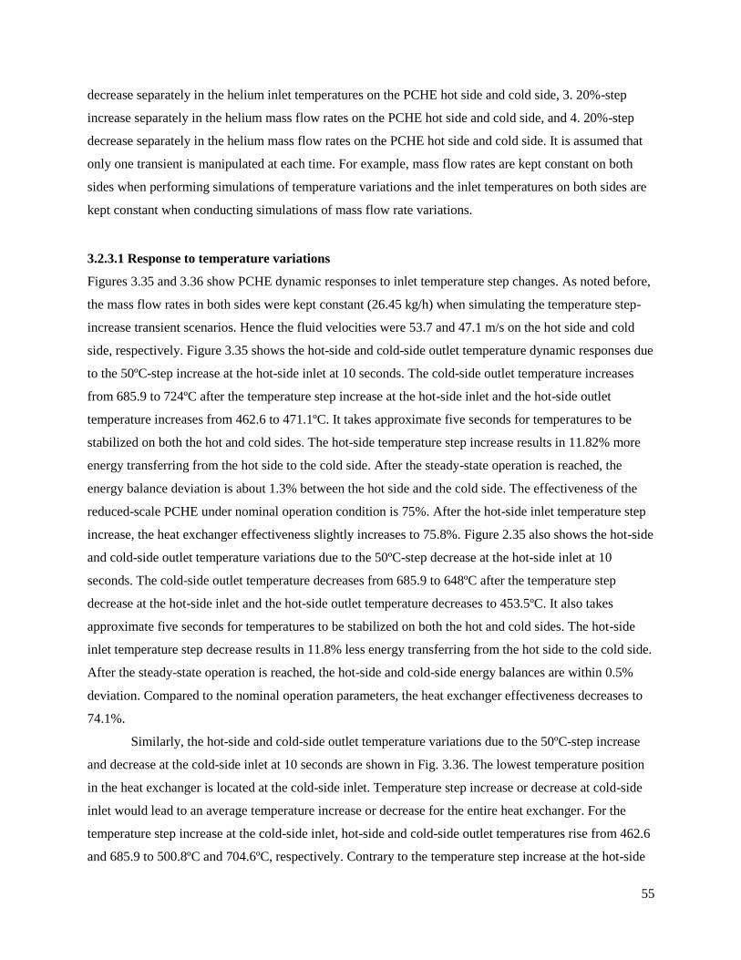
55
decrease separately in the helium inlet temperatures on the PCHE hot side and cold side, 3. 20%-step
increase separately in the helium mass flow rates on the PCHE hot side and cold side, and 4. 20%-step
decrease separately in the helium mass flow rates on the PCHE hot side and cold side. It is assumed that
only one transient is manipulated at each time. For example, mass flow rates are kept constant on both
sides when performing simulations of temperature variations and the inlet temperatures on both sides are
kept constant when conducting simulations of mass flow rate variations.
3.2.3.1 Response to temperature variations
Figures 3.35 and 3.36 show PCHE dynamic responses to inlet temperature step changes. As noted before,
the mass flow rates in both sides were kept constant (26.45 kg/h) when simulating the temperature step-
increase transient scenarios. Hence the fluid velocities were 53.7 and 47.1 m/s on the hot side and cold
side, respectively. Figure 3.35 shows the hot-side and cold-side outlet temperature dynamic responses due
to the 50ºC-step increase at the hot-side inlet at 10 seconds. The cold-side outlet temperature increases
from 685.9 to 724ºC after the temperature step increase at the hot-side inlet and the hot-side outlet
temperature increases from 462.6 to 471.1ºC. It takes approximate five seconds for temperatures to be
stabilized on both the hot and cold sides. The hot-side temperature step increase results in 11.82% more
energy transferring from the hot side to the cold side. After the steady-state operation is reached, the
energy balance deviation is about 1.3% between the hot side and the cold side. The effectiveness of the
reduced-scale PCHE under nominal operation condition is 75%. After the hot-side inlet temperature step
increase, the heat exchanger effectiveness slightly increases to 75.8%. Figure 2.35 also shows the hot-side
and cold-side outlet temperature variations due to the 50ºC-step decrease at the hot-side inlet at 10
seconds. The cold-side outlet temperature decreases from 685.9 to 648ºC after the temperature step
decrease at the hot-side inlet and the hot-side outlet temperature decreases to 453.5ºC. It also takes
approximate five seconds for temperatures to be stabilized on both the hot and cold sides. The hot-side
inlet temperature step decrease results in 11.8% less energy transferring from the hot side to the cold side.
After the steady-state operation is reached, the hot-side and cold-side energy balances are within 0.5%
deviation. Compared to the nominal operation parameters, the heat exchanger effectiveness decreases to
74.1%.
Similarly, the hot-side and cold-side outlet temperature variations due to the 50ºC-step increase
and decrease at the cold-side inlet at 10 seconds are shown in Fig. 3.36. The lowest temperature position
in the heat exchanger is located at the cold-side inlet. Temperature step increase or decrease at cold-side
inlet would lead to an average temperature increase or decrease for the entire heat exchanger. For the
temperature step increase at the cold-side inlet, hot-side and cold-side outlet temperatures rise from 462.6
and 685.9 to 500.8ºC and 704.6ºC, respectively. Contrary to the temperature step increase at the hot-side
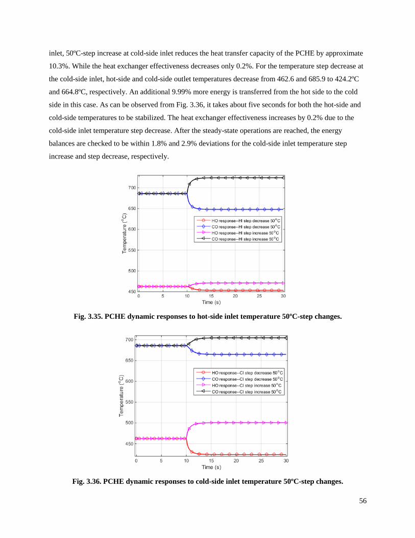
56
inlet, 50ºC-step increase at cold-side inlet reduces the heat transfer capacity of the PCHE by approximate
10.3%. While the heat exchanger effectiveness decreases only 0.2%. For the temperature step decrease at
the cold-side inlet, hot-side and cold-side outlet temperatures decrease from 462.6 and 685.9 to 424.2ºC
and 664.8ºC, respectively. An additional 9.99% more energy is transferred from the hot side to the cold
side in this case. As can be observed from Fig. 3.36, it takes about five seconds for both the hot-side and
cold-side temperatures to be stabilized. The heat exchanger effectiveness increases by 0.2% due to the
cold-side inlet temperature step decrease. After the steady-state operations are reached, the energy
balances are checked to be within 1.8% and 2.9% deviations for the cold-side inlet temperature step
increase and step decrease, respectively.
Fig. 3.35. PCHE dynamic responses to hot-side inlet temperature 50ºC-step changes.
Fig. 3.36. PCHE dynamic responses to cold-side inlet temperature 50ºC-step changes.
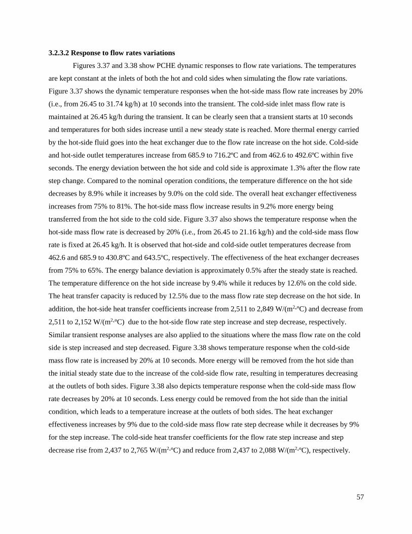
57
3.2.3.2 Response to flow rates variations
Figures 3.37 and 3.38 show PCHE dynamic responses to flow rate variations. The temperatures
are kept constant at the inlets of both the hot and cold sides when simulating the flow rate variations.
Figure 3.37 shows the dynamic temperature responses when the hot-side mass flow rate increases by 20%
(i.e., from 26.45 to 31.74 kg/h) at 10 seconds into the transient. The cold-side inlet mass flow rate is
maintained at 26.45 kg/h during the transient. It can be clearly seen that a transient starts at 10 seconds
and temperatures for both sides increase until a new steady state is reached. More thermal energy carried
by the hot-side fluid goes into the heat exchanger due to the flow rate increase on the hot side. Cold-side
and hot-side outlet temperatures increase from 685.9 to 716.2ºC and from 462.6 to 492.6ºC within five
seconds. The energy deviation between the hot side and cold side is approximate 1.3% after the flow rate
step change. Compared to the nominal operation conditions, the temperature difference on the hot side
decreases by 8.9% while it increases by 9.0% on the cold side. The overall heat exchanger effectiveness
increases from 75% to 81%. The hot-side mass flow increase results in 9.2% more energy being
transferred from the hot side to the cold side. Figure 3.37 also shows the temperature response when the
hot-side mass flow rate is decreased by 20% (i.e., from 26.45 to 21.16 kg/h) and the cold-side mass flow
rate is fixed at 26.45 kg/h. It is observed that hot-side and cold-side outlet temperatures decrease from
462.6 and 685.9 to 430.8ºC and 643.5ºC, respectively. The effectiveness of the heat exchanger decreases
from 75% to 65%. The energy balance deviation is approximately 0.5% after the steady state is reached.
The temperature difference on the hot side increase by 9.4% while it reduces by 12.6% on the cold side.
The heat transfer capacity is reduced by 12.5% due to the mass flow rate step decrease on the hot side. In
addition, the hot-side heat transfer coefficients increase from 2,511 to 2,849 W/(m2∙ºC) and decrease from
2,511 to 2,152 W/(m2∙ºC) due to the hot-side flow rate step increase and step decrease, respectively.
Similar transient response analyses are also applied to the situations where the mass flow rate on the cold
side is step increased and step decreased. Figure 3.38 shows temperature response when the cold-side
mass flow rate is increased by 20% at 10 seconds. More energy will be removed from the hot side than
the initial steady state due to the increase of the cold-side flow rate, resulting in temperatures decreasing
at the outlets of both sides. Figure 3.38 also depicts temperature response when the cold-side mass flow
rate decreases by 20% at 10 seconds. Less energy could be removed from the hot side than the initial
condition, which leads to a temperature increase at the outlets of both sides. The heat exchanger
effectiveness increases by 9% due to the cold-side mass flow rate step decrease while it decreases by 9%
for the step increase. The cold-side heat transfer coefficients for the flow rate step increase and step
decrease rise from 2,437 to 2,765 W/(m2∙ºC) and reduce from 2,437 to 2,088 W/(m2∙ºC), respectively.
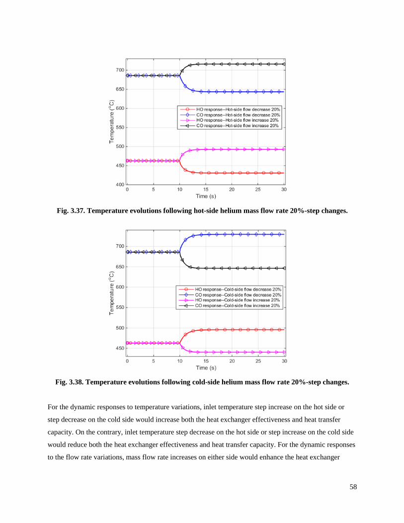
58
Fig. 3.37. Temperature evolutions following hot-side helium mass flow rate 20%-step changes.
Fig. 3.38. Temperature evolutions following cold-side helium mass flow rate 20%-step changes.
For the dynamic responses to temperature variations, inlet temperature step increase on the hot side or
step decrease on the cold side would increase both the heat exchanger effectiveness and heat transfer
capacity. On the contrary, inlet temperature step decrease on the hot side or step increase on the cold side
would reduce both the heat exchanger effectiveness and heat transfer capacity. For the dynamic responses
to the flow rate variations, mass flow rate increases on either side would enhance the heat exchanger
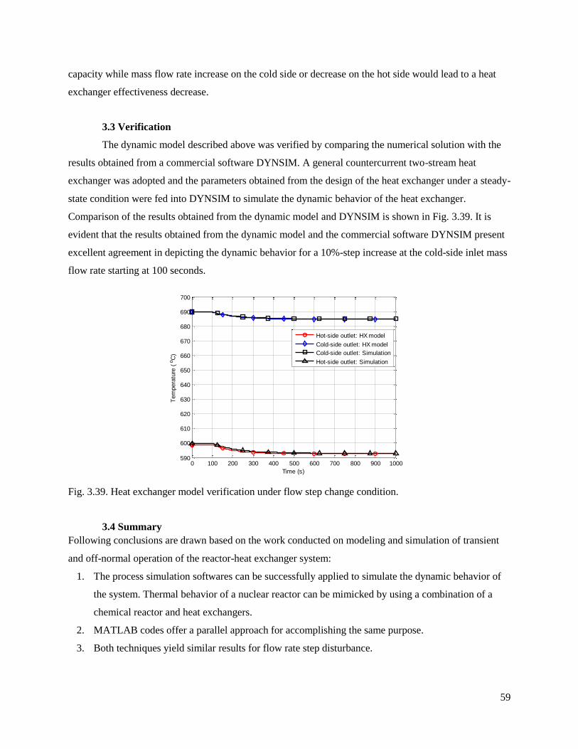
59
capacity while mass flow rate increase on the cold side or decrease on the hot side would lead to a heat
exchanger effectiveness decrease.
3.3 Verification
The dynamic model described above was verified by comparing the numerical solution with the
results obtained from a commercial software DYNSIM. A general countercurrent two-stream heat
exchanger was adopted and the parameters obtained from the design of the heat exchanger under a steady-
state condition were fed into DYNSIM to simulate the dynamic behavior of the heat exchanger.
Comparison of the results obtained from the dynamic model and DYNSIM is shown in Fig. 3.39. It is
evident that the results obtained from the dynamic model and the commercial software DYNSIM present
excellent agreement in depicting the dynamic behavior for a 10%-step increase at the cold-side inlet mass
flow rate starting at 100 seconds.
Fig. 3.39. Heat exchanger model verification under flow step change condition.
3.4 Summary
Following conclusions are drawn based on the work conducted on modeling and simulation of transient
and off-normal operation of the reactor-heat exchanger system:
1. The process simulation softwares can be successfully applied to simulate the dynamic behavior of
the system. Thermal behavior of a nuclear reactor can be mimicked by using a combination of a
chemical reactor and heat exchangers.
2. MATLAB codes offer a parallel approach for accomplishing the same purpose.
3. Both techniques yield similar results for flow rate step disturbance.
0 100 200 300 400 500 600 700 800 900 1000590
600
610
620
630
640
650
660
670
680
690
700
Time (s)
Tem
pera
ture
( o
C)
Hot-side outlet: HX model
Cold-side outlet: HX model
Cold-side outlet: Simulation
Hot-side outlet: Simulation
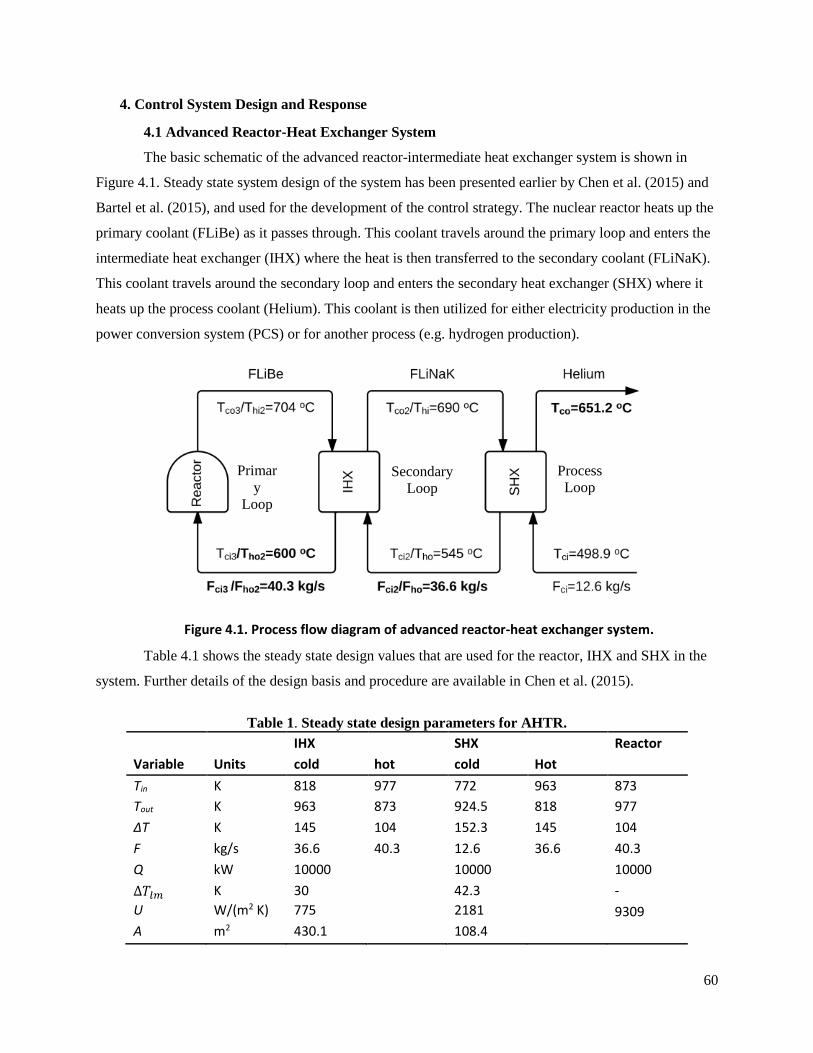
60
4. Control System Design and Response
4.1 Advanced Reactor-Heat Exchanger System
The basic schematic of the advanced reactor-intermediate heat exchanger system is shown in
Figure 4.1. Steady state system design of the system has been presented earlier by Chen et al. (2015) and
Bartel et al. (2015), and used for the development of the control strategy. The nuclear reactor heats up the
primary coolant (FLiBe) as it passes through. This coolant travels around the primary loop and enters the
intermediate heat exchanger (IHX) where the heat is then transferred to the secondary coolant (FLiNaK).
This coolant travels around the secondary loop and enters the secondary heat exchanger (SHX) where it
heats up the process coolant (Helium). This coolant is then utilized for either electricity production in the
power conversion system (PCS) or for another process (e.g. hydrogen production).
Figure 4.1. Process flow diagram of advanced reactor-heat exchanger system.
Table 4.1 shows the steady state design values that are used for the reactor, IHX and SHX in the
system. Further details of the design basis and procedure are available in Chen et al. (2015).
Table 1. Steady state design parameters for AHTR. IHX SHX Reactor
Variable Units cold hot cold Hot
Tin K 818 977 772 963 873
Tout K 963 873 924.5 818 977
ΔT K 145 104 152.3 145 104
F kg/s 36.6 40.3 12.6 36.6 40.3
Q kW 10000 10000 10000
∆𝑇𝑙𝑚 K 30 42.3 -
U W/(m2 K) 775 2181 9309
A m2 430.1 108.4
Primar
y
Loop
Secondary
Loop
Process
Loop

61
4.2 Helium Brayton Cycle Power Conversion System (PCS)
The generalized schematic shown above assumes that the heat transferred out of the SHX into the process
loop can be utilized for either direct application in a process or converted to electricity via a power
generation cycle. It is assumed that, for the advanced reactor-heat exchanger system described above, the
power conversion system (PCS) involves a helium Brayton cycle shown below in Figure 4.2.
Figure 4.2. Helium Brayton cycle schematic.
The coolant, helium, exits the SHX at a high temperature and enters the turbine. The energy from the
turbine spins a generator in which electricity is produced. The pressure drops as the coolant travels
through the turbine. The helium enters a recuperator in which the cold side stream exiting the compressor
is heated up. Helium then travels through a precooler where water is used to cool down the helium before
entering the compressor. Helium enters the compressor where the temperature and pressure of the coolant
increase. Compressed helium travels through the recuperator heating up to the desired temperature before
entering the SHX again. Control of the helium temperature exiting the SHX is of upmost importance
because it has an effect on the overall efficiency of the Brayton cycle.
4.3 Control System Architecture
Creating a control strategy to maintain high system efficiencies requires developing and
designing a control system architecture for the system. Figure 4.3 shows a possible control system
architecture for the system.

62
Figure 4.3. Possible design for control of AHTR system.
4.3.1 Control Methodology
The first step in the design of a control system is the identification and selection of the controlled
variables (variables maintained at desired set-point values) and manipulated variables (variables changed
in order to maintain the controlled variables at their set points). For the SHX, the controlled variable was
chosen to be the cold side outlet temperature (Tco) of the process coolant. The process coolant travels
through the process loop and is used either to generate electricity or provide thermal energy to drive a
chemical process. Processes are designed to operate at specified temperatures, and the temperature
difference between the process coolant and design temperature provides the necessary driving force for its
operation. Controlling the process coolant temperature (Tco) will maintain the necessary driving force at
the desired value, enabling the process to operate at the optimum efficiency. This control is accomplished
by using the hot side flow rate (Fhi) or the cold side flow rate (Fci) as the manipulated variable. Other
variables, called load variables, represent disturbances that will have an effect on the controlled variable.
For the SHX, the load variables include the hot and cold inlet temperatures (Thi, Tci) and the flow rate that
is not the manipulated variable (Fci or Fhi).
The controlled variable for IHX was the hot side outlet temperature (Tho2). This is the temperature
of the primary coolant entering the nuclear reactor. Fluctuations in this temperature will have an effect on
the reactivity and thus the power of the reactor, which is undesirable. The hot side flow rate (Fhi2) or the
cold side flow rate (Fci2) is used as the manipulated variable. The load variables include the hot and cold
inlet temperatures (Thi2, Tci2) and the flow rate that is not the manipulated variable (Fci2 or Fhi2). It is
important to note that if Fci2 is the manipulated variable of the IHX, Fci must be the manipulated variable
for the SHX because Fci2 and Fhi are the same flow rate.
The controlled variable for the reactor was the neutron density (n) which is proportional to reactor
power. The neutron density is controlled by manipulating the reactivity with control rod movement (ρrod).
The load variable of the reactor are the coolant mass flow rate (Fc), the reactor inlet temperature (Ti), the

63
reactor outlet temperature (Te), and the fuel temperature (Tf). Table 4.2 shows the controlled,
manipulated, and load variables for each of the units in the system.
Table 4.2. Summary of controlled, manipulated and load variables.
Process
Unit
Controlled
Variable
Manipulated
Variable
Load
Variables
SHX Tco Fhi or Fci Fci or Fhi, Tci, Thi
IHX Tho2 Fhi2 or Fci2 Fci2 or Fhi2, Tci2, Thi2
Reactor n ρrod Fc, Ti, Te, Tf
4.3.2 Block Diagrams
Control block diagrams were created to represent the control strategy for each heat exchanger.
Figures 4.4 and 4.5 show the block diagrams for the SHX and IHX, respectively. Each block in these
figures represents a transfer function which relates the variables entering and leaving the block. Each
variable within the block is expressed as the deviation from the steady state values of that particular
parameter. For example, the topmost block in Figure 4.4 relates the deviation in the cold stream outlet
temperature (Tco) from its steady state value to the deviation in the temperature of the hot inlet stream
(Thi) from its steady state value. These two deviations are related by the transfer function GS4. The
asterisk on a variable (for example, Tco*) indicates a set-point value which is 0. Both the block diagrams
are structured identically, differing only in the controlled and manipulated variables, and the transfer
functions. For each diagram Gc is the controller transfer function, Gv is the valve or pump transfer
function and GS/GI are the process transfer functions for the SHX and IHX, respectively.
The process transfer functions (GS/GI) represent the mathematical relationships between the
controlled variables and the manipulated variable or load variables. Referring to Figure 4.4, the transfer
functions GS2, GS3 and GS4 represent the transfer functions which effectively convert the deviations (or
disturbances) in the load variables Fci, Tci and Thi, respectively, to the deviation in the controlled variable
Tco. GS1 is the transfer function between the controlled (Tco) and the manipulated variable (Fhi). All the
deviations are summed up at the summation point at the right end of the figure, and total deviation is
compared to the set-point at the summation junction at the left end of the figure. The error signal (E1)
generated is sent to the controller (GcS). Depending on the error and the controller algorithm, the
controller sends an output signal (P1) to the valve transfer function block. The manipulated variable Fhi is
changed based on the valve transfer function (GvS), to keep the controlled variable at its desired value.
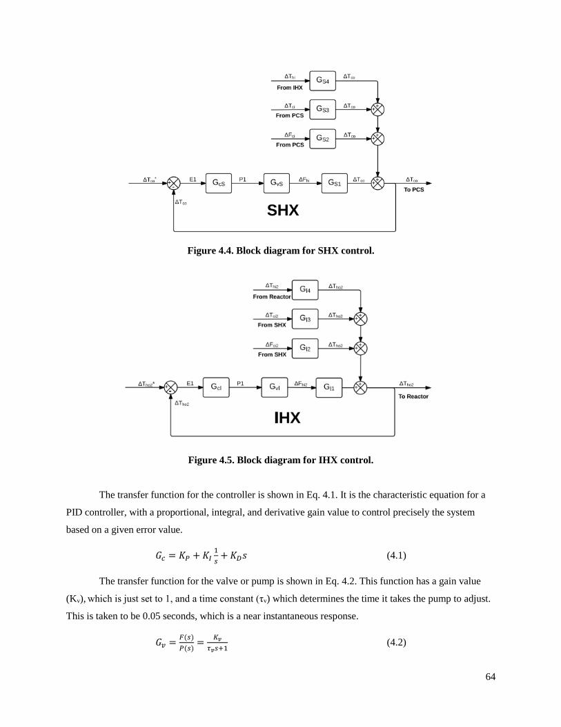
64
Figure 4.4. Block diagram for SHX control.
Figure 4.5. Block diagram for IHX control.
The transfer function for the controller is shown in Eq. 4.1. It is the characteristic equation for a
PID controller, with a proportional, integral, and derivative gain value to control precisely the system
based on a given error value.
𝐺𝑐 = 𝐾𝑃 + 𝐾𝐼1
𝑠+ 𝐾𝐷𝑠 (4.1)
The transfer function for the valve or pump is shown in Eq. 4.2. This function has a gain value
(Kv), which is just set to 1, and a time constant (τv) which determines the time it takes the pump to adjust.
This is taken to be 0.05 seconds, which is a near instantaneous response.
𝐺𝑣 =𝐹(𝑠)
𝑃(𝑠)=
𝐾𝑣
𝜏𝑣𝑠+1 (4.2)
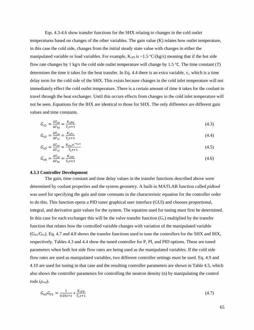
65
Eqs. 4.3-4.6 show transfer functions for the SHX relating to changes in the cold outlet
temperatures based on changes of the other variables. The gain value (K) relates how outlet temperature,
in this case the cold side, changes from the initial steady state value with changes in either the
manipulated variable or load variables. For example, KcFh is ~1.5 oC/(kg/s) meaning that if the hot side
flow rate changes by 1 kg/s the cold side outlet temperature will change by 1.5 oC. The time constant (T)
determines the time it takes for the heat transfer. In Eq. 4.4 there is an extra variable, τc, which is a time
delay term for the cold side of the SHX. This exists because changes in the cold inlet temperature will not
immediately effect the cold outlet temperature. There is a certain amount of time it takes for the coolant to
travel through the heat exchanger. Until this occurs effects from changes in the cold inlet temperature will
not be seen. Equations for the IHX are identical to those for SHX. The only difference are different gain
values and time constants.
𝐺𝑠1 =∆𝑇𝑐𝑜
∆𝐹ℎ𝑖=
𝐾𝑐𝐹ℎ
𝑇𝑐𝑠+1 (4.3)
𝐺𝑠2 =∆𝑇𝑐𝑜
∆𝐹𝑐𝑖=
𝐾𝑐𝐹𝑐
𝑇𝑐𝑠+1 (4.4)
𝐺𝑠3 =∆𝑇𝑐𝑜
∆𝑇𝑐𝑖=
𝐾𝑐𝑡𝑐𝑒−𝜏𝑐𝑠
𝑇𝑐𝑠+1 (4.5)
𝐺𝑠4 =∆𝑇𝑐𝑜
∆𝑇ℎ𝑖=
𝐾𝑐𝑡ℎ
𝑇𝑐𝑠+1 (4.6)
4.3.3 Controller Development
The gain, time constant and time delay values in the transfer functions described above were
determined by coolant properties and the system geometry. A built-in MATLAB function called pidtool
was used for specifying the gain and time constants in the characteristic equation for the controller order
to do this. This function opens a PID tuner graphical user interface (GUI) and chooses proportional,
integral, and derivative gain values for the system. The equation used for tuning must first be determined.
In this case for each exchanger this will be the valve transfer function (Gv) multiplied by the transfer
function that relates how the controlled variable changes with variation of the manipulated variable
(GS1/GI1). Eq. 4.7 and 4.8 shows the transfer functions used to tune the controllers for the SHX and IHX,
respectively. Tables 4.3 and 4.4 show the tuned controller for P, PI, and PID options. These are tuned
parameters when both hot side flow rates are being used as the manipulated variables. If the cold side
flow rates are used as manipulated variables, two different controller settings must be used. Eq. 4.9 and
4.10 are used for tuning in that case and the resulting controller parameters are shown in Table 4.5, which
also shows the controller parameters for controlling the neutron density (n) by manipulating the control
rods (ρrod).
𝐺𝑣𝑆𝐺𝑆1 =1
0.05𝑠+1∗
𝐾𝑐𝐹ℎ
𝑇𝑐𝑠+1 (4.7)
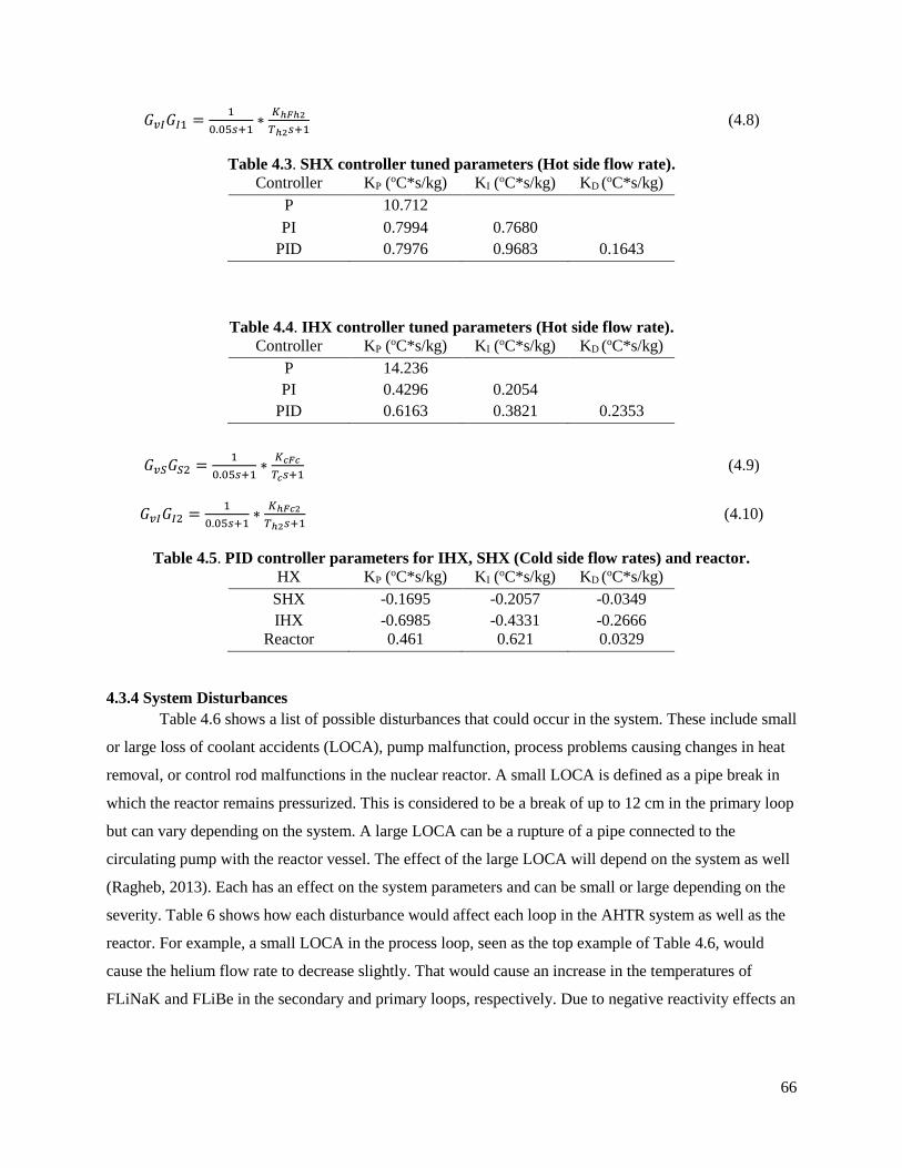
66
𝐺𝑣𝐼𝐺𝐼1 =1
0.05𝑠+1∗
𝐾ℎ𝐹ℎ2
𝑇ℎ2𝑠+1 (4.8)
Table 4.3. SHX controller tuned parameters (Hot side flow rate).
Controller KP (oC*s/kg) KI (oC*s/kg) KD (oC*s/kg)
P 10.712
PI 0.7994 0.7680
PID 0.7976 0.9683 0.1643
Table 4.4. IHX controller tuned parameters (Hot side flow rate).
Controller KP (oC*s/kg) KI (oC*s/kg) KD (oC*s/kg)
P 14.236
PI 0.4296 0.2054
PID 0.6163 0.3821 0.2353
𝐺𝑣𝑆𝐺𝑆2 =1
0.05𝑠+1∗
𝐾𝑐𝐹𝑐
𝑇𝑐𝑠+1 (4.9)
𝐺𝑣𝐼𝐺𝐼2 =1
0.05𝑠+1∗
𝐾ℎ𝐹𝑐2
𝑇ℎ2𝑠+1 (4.10)
Table 4.5. PID controller parameters for IHX, SHX (Cold side flow rates) and reactor.
HX KP (oC*s/kg) KI (oC*s/kg) KD (oC*s/kg)
SHX -0.1695 -0.2057 -0.0349
IHX -0.6985 -0.4331 -0.2666
Reactor 0.461 0.621 0.0329
4.3.4 System Disturbances
Table 4.6 shows a list of possible disturbances that could occur in the system. These include small
or large loss of coolant accidents (LOCA), pump malfunction, process problems causing changes in heat
removal, or control rod malfunctions in the nuclear reactor. A small LOCA is defined as a pipe break in
which the reactor remains pressurized. This is considered to be a break of up to 12 cm in the primary loop
but can vary depending on the system. A large LOCA can be a rupture of a pipe connected to the
circulating pump with the reactor vessel. The effect of the large LOCA will depend on the system as well
(Ragheb, 2013). Each has an effect on the system parameters and can be small or large depending on the
severity. Table 6 shows how each disturbance would affect each loop in the AHTR system as well as the
reactor. For example, a small LOCA in the process loop, seen as the top example of Table 4.6, would
cause the helium flow rate to decrease slightly. That would cause an increase in the temperatures of
FLiNaK and FLiBe in the secondary and primary loops, respectively. Due to negative reactivity effects an

67
increase in FLiBe temperature entering the reactor would cause a decrease in the power output of the
reactor.
Table 4.6. Possible disturbances and their effects on the system.
Disturbance Process Effect Secondary Effect Primary Effect Reactor Effect
1. Small LOCA in process loop
Lower helium flowrate (T ↑)
Higher FLiNaK temperature
Higher FLiBe temperature
Lower reactor duty
2. Large LOCA in process loop
Much Lower helium flowrate (T ↑)
Much Higher FLiNaK temperature
Much Higher FLiBe temperature
Much Lower reactor duty
3. Small LOCA in secondary loop
Lower helium temperature
Lower secondary flowrate
Higher FLiBe temperature
Lower reactor duty
4. Large LOCA in secondary loop
Much Lower helium temperature
Much Lower secondary flowrate
Much Higher FLiBe temperature
Much Lower reactor duty
5. Small LOCA in primary loop
Lower helium temperature
Lower FLiNaK temperature
Lower primary flowrate
Lower/higher reactor duty
6. Large LOCA in primary loop
Much Lower helium temperature
Much Lower FLiNaK temperature
Much Lower primary flowrate
Much Lower reactor duty
7. Process pump malfunction(2)
Higher helium flowrate (T ↓)
Lower FLiNaK temperature
Lower FLiBe temperature
Higher reactor duty
8. Secondary pump malfunction(2)
Higher helium temperature
Higher secondary flowrate
Lower FLiBe temperature
Higher reactor duty
9. Primary pump malfunction(2)
Higher helium temperature
Higher FLiNaK temperature
Higher primary flowrate
Lower/higher reactor duty
10. Lower process heat removal
Higher helium temperature
Higher FLiNaK temperature
Higher FLiBe temperature
Lower reactor duty
11. Higher process heat removal
Lower helium temperature
Lower FLiNaK temperature
Lower FLiBe temperature
Lower reactor duty
12. Control rod malfunction(ρrod ↑)
Higher helium temperature
Higher FLiNaK temperature
Higher FLiBe temperature
Initial higher reactor duty.
13. Control rod malfunction(ρrod ↓)
Lower helium temperature
Lower FLiNaK temperature
Lower FLiBe temperature
Initial lower reactor duty
4.4 System Models and Simulation Technique
4.4.1 Governing Equations for Heat Exchangers
The representative governing equations for a heat exchanger were obtained by the energy balance
and are shown Eqs. 4.11-4.13. Eq. 4.11 is the energy balance for the hot stream, Eq. 4.12 is the energy
balance for the cold stream, and Eq. 4.13 represents the energy balance for the wall separating the two
streams, written for a differential element of the heat exchanger.
𝑚ℎ𝐶𝑝ℎ𝑑𝑇ℎ
𝑑𝑡+ 𝐹ℎ𝐶𝑝ℎ(𝑇ℎ𝑜 − 𝑇ℎ𝑖) = (ℎ𝐴)ℎ(𝑇𝑤 − 𝑇ℎ) (4.11)
𝑚𝑐𝐶𝑝𝑐𝑑𝑇𝑐
𝑑𝑡+ 𝐹𝑐𝐶𝑝𝑐(𝑇𝑐𝑜 − 𝑇𝑐𝑖) = (ℎ𝐴)𝑐(𝑇𝑤 − 𝑇𝑐) (4.12)
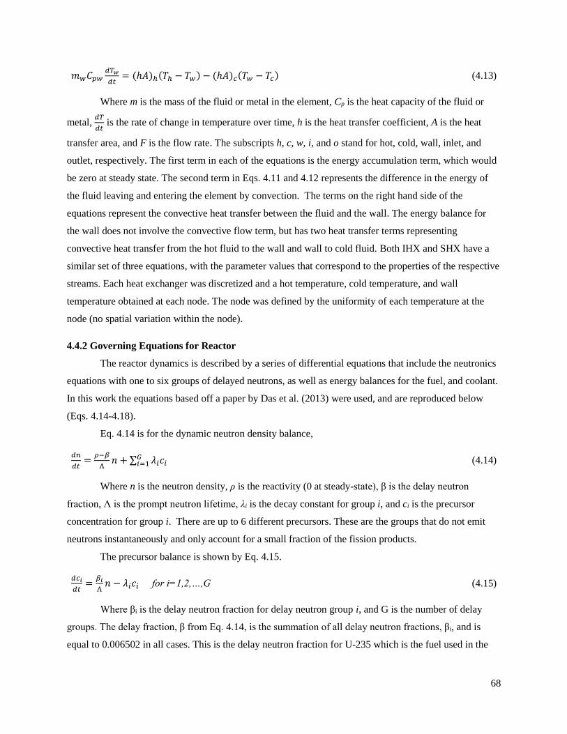
68
𝑚𝑤𝐶𝑝𝑤𝑑𝑇𝑤
𝑑𝑡= (ℎ𝐴)ℎ(𝑇ℎ − 𝑇𝑤) − (ℎ𝐴)𝑐(𝑇𝑤 − 𝑇𝑐) (4.13)
Where m is the mass of the fluid or metal in the element, Cp is the heat capacity of the fluid or
metal, 𝑑𝑇
𝑑𝑡 is the rate of change in temperature over time, h is the heat transfer coefficient, A is the heat
transfer area, and F is the flow rate. The subscripts h, c, w, i, and o stand for hot, cold, wall, inlet, and
outlet, respectively. The first term in each of the equations is the energy accumulation term, which would
be zero at steady state. The second term in Eqs. 4.11 and 4.12 represents the difference in the energy of
the fluid leaving and entering the element by convection. The terms on the right hand side of the
equations represent the convective heat transfer between the fluid and the wall. The energy balance for
the wall does not involve the convective flow term, but has two heat transfer terms representing
convective heat transfer from the hot fluid to the wall and wall to cold fluid. Both IHX and SHX have a
similar set of three equations, with the parameter values that correspond to the properties of the respective
streams. Each heat exchanger was discretized and a hot temperature, cold temperature, and wall
temperature obtained at each node. The node was defined by the uniformity of each temperature at the
node (no spatial variation within the node).
4.4.2 Governing Equations for Reactor
The reactor dynamics is described by a series of differential equations that include the neutronics
equations with one to six groups of delayed neutrons, as well as energy balances for the fuel, and coolant.
In this work the equations based off a paper by Das et al. (2013) were used, and are reproduced below
(Eqs. 4.14-4.18).
Eq. 4.14 is for the dynamic neutron density balance,
𝑑𝑛
𝑑𝑡=
𝜌−𝛽
Λ𝑛 + ∑ 𝜆𝑖𝑐𝑖
𝐺𝑖=1 (4.14)
Where n is the neutron density, ρ is the reactivity (0 at steady-state), β is the delay neutron
fraction, Λ is the prompt neutron lifetime, λi is the decay constant for group i, and ci is the precursor
concentration for group i. There are up to 6 different precursors. These are the groups that do not emit
neutrons instantaneously and only account for a small fraction of the fission products.
The precursor balance is shown by Eq. 4.15.
𝑑𝑐𝑖
𝑑𝑡=
𝛽𝑖
Λ𝑛 − 𝜆𝑖𝑐𝑖 for i=1,2,…,G (4.15)
Where βi is the delay neutron fraction for delay neutron group i, and G is the number of delay
groups. The delay fraction, β from Eq. 4.14, is the summation of all delay neutron fractions, βi, and is
equal to 0.006502 in all cases. This is the delay neutron fraction for U-235 which is the fuel used in the
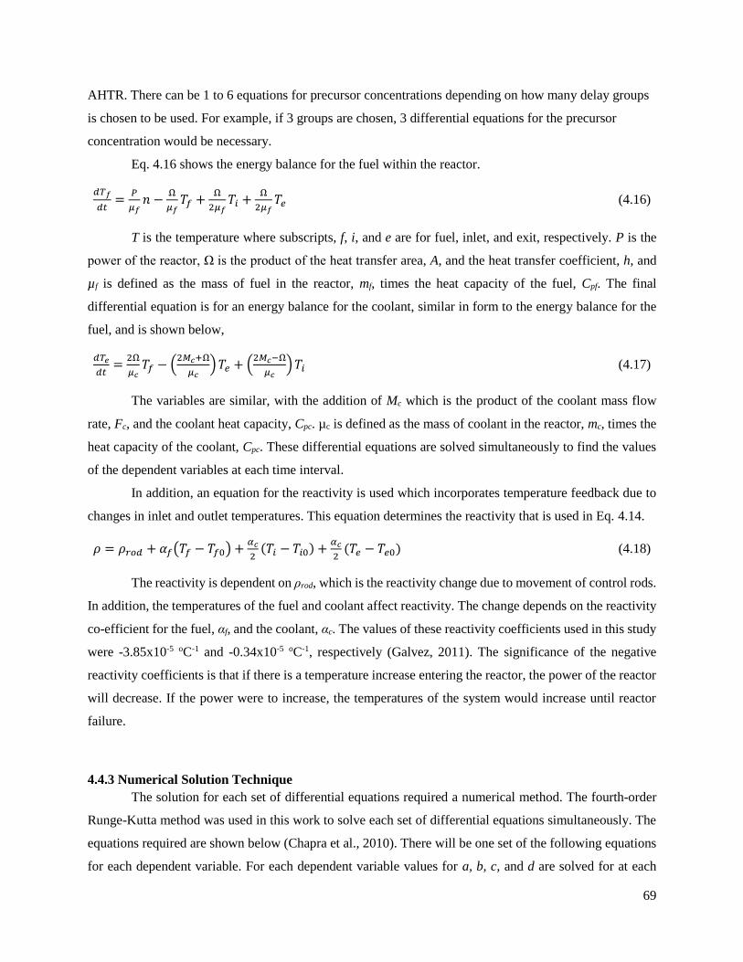
69
AHTR. There can be 1 to 6 equations for precursor concentrations depending on how many delay groups
is chosen to be used. For example, if 3 groups are chosen, 3 differential equations for the precursor
concentration would be necessary.
Eq. 4.16 shows the energy balance for the fuel within the reactor.
𝑑𝑇𝑓
𝑑𝑡=
𝑃
𝜇𝑓𝑛 −
Ω
𝜇𝑓𝑇𝑓 +
Ω
2𝜇𝑓𝑇𝑖 +
Ω
2𝜇𝑓𝑇𝑒 (4.16)
T is the temperature where subscripts, f, i, and e are for fuel, inlet, and exit, respectively. P is the
power of the reactor, Ω is the product of the heat transfer area, A, and the heat transfer coefficient, h, and
µf is defined as the mass of fuel in the reactor, mf, times the heat capacity of the fuel, Cpf. The final
differential equation is for an energy balance for the coolant, similar in form to the energy balance for the
fuel, and is shown below,
𝑑𝑇𝑒
𝑑𝑡=
2Ω
𝜇𝑐𝑇𝑓 − (
2𝑀𝑐+Ω
𝜇𝑐) 𝑇𝑒 + (
2𝑀𝑐−Ω
𝜇𝑐) 𝑇𝑖 (4.17)
The variables are similar, with the addition of Mc which is the product of the coolant mass flow
rate, Fc, and the coolant heat capacity, Cpc. µc is defined as the mass of coolant in the reactor, mc, times the
heat capacity of the coolant, Cpc. These differential equations are solved simultaneously to find the values
of the dependent variables at each time interval.
In addition, an equation for the reactivity is used which incorporates temperature feedback due to
changes in inlet and outlet temperatures. This equation determines the reactivity that is used in Eq. 4.14.
𝜌 = 𝜌𝑟𝑜𝑑 + 𝛼𝑓(𝑇𝑓 − 𝑇𝑓0) +𝛼𝑐
2(𝑇𝑖 − 𝑇𝑖0) +
𝛼𝑐
2(𝑇𝑒 − 𝑇𝑒0) (4.18)
The reactivity is dependent on ρrod, which is the reactivity change due to movement of control rods.
In addition, the temperatures of the fuel and coolant affect reactivity. The change depends on the reactivity
co-efficient for the fuel, αf, and the coolant, αc. The values of these reactivity coefficients used in this study
were -3.85x10⁻⁵ oC-1 and -0.34x10⁻⁵ oC-1, respectively (Galvez, 2011). The significance of the negative
reactivity coefficients is that if there is a temperature increase entering the reactor, the power of the reactor
will decrease. If the power were to increase, the temperatures of the system would increase until reactor
failure.
4.4.3 Numerical Solution Technique
The solution for each set of differential equations required a numerical method. The fourth-order
Runge-Kutta method was used in this work to solve each set of differential equations simultaneously. The
equations required are shown below (Chapra et al., 2010). There will be one set of the following equations
for each dependent variable. For each dependent variable values for a, b, c, and d are solved for at each
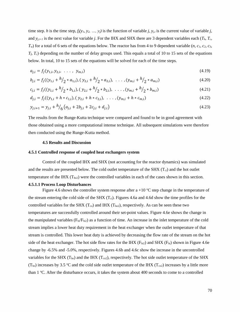
70
time step. h is the time step, fj(y1, y2, …, yj) is the function of variable j, yj,i is the current value of variable j,
and yj,i+1 is the next value for variable j. For the IHX and SHX there are 3 dependent variables each (Th, Tc,
Tw) for a total of 6 sets of the equations below. The reactor has from 4 to 9 dependent variable (n, c1, c2, c3,
Tf, Tc) depending on the number of delay groups used. This equals a total of 10 to 15 sets of the equations
below. In total, 10 to 15 sets of the equations will be solved for each of the time steps.
𝑎𝑗,𝑖 = 𝑓𝑗(𝑦1,𝑖, 𝑦2,𝑖, . . . , 𝑦𝑚,𝑖) (4.19)
𝑏𝑗,𝑖 = 𝑓𝑗((𝑦1,𝑖 + ℎ2⁄ ∗ 𝑎1,𝑖), ( 𝑦2,𝑖 + ℎ
2⁄ ∗ 𝑎2,𝑖), . . . , (𝑦𝑚,𝑖 + ℎ2⁄ ∗ 𝑎𝑚,𝑖) (4.20)
𝑐𝑗,𝑖 = 𝑓𝑗((𝑦1,𝑖 + ℎ2⁄ ∗ 𝑏1,𝑖), ( 𝑦2,𝑖 + ℎ
2⁄ ∗ 𝑏2,𝑖), . . . , (𝑦𝑚,𝑖 + ℎ2⁄ ∗ 𝑏𝑚,𝑖) (4.21)
𝑑𝑗,𝑖 = 𝑓𝑗((𝑦1,𝑖 + ℎ ∗ 𝑐1,𝑖), ( 𝑦2,𝑖 + ℎ ∗ 𝑐2,𝑖), . . . , (𝑦𝑚,𝑖 + ℎ ∗ 𝑐𝑚,𝑖) (4.22)
𝑦𝑗,𝑖+1 = 𝑦𝑗,𝑖 + ℎ6⁄ (𝑎𝑗,𝑖 + 2𝑏𝑗,𝑖 + 2𝑐𝑗,𝑖 + 𝑑𝑗,𝑖) (4.23)
The results from the Runge-Kutta technique were compared and found to be in good agreement with
those obtained using a more computational intense technique. All subsequent simulations were therefore
then conducted using the Runge-Kutta method.
4.5 Results and Discussion
4.5.1 Controlled response of coupled heat exchangers system
Control of the coupled IHX and SHX (not accounting for the reactor dynamics) was simulated
and the results are presented below. The cold outlet temperature of the SHX (Tci) and the hot outlet
temperature of the IHX (Tho2) were the controlled variables in each of the cases shown in this section.
4.5.1.1 Process Loop Disturbances
Figure 4.6 shows the controller system response after a +10 oC step change in the temperature of
the stream entering the cold side of the SHX (Tci). Figures 4.6a and 4.6d show the time profiles for the
controlled variables for the SHX (Tco) and IHX (Tho2), respectively. As can be seen these two
temperatures are successfully controlled around their set-point values. Figure 4.6e shows the change in
the manipulated variables (Fhi/Fhi2) as a function of time. An increase in the inlet temperature of the cold
stream implies a lower heat duty requirement in the heat exchanger when the outlet temperature of that
stream is controlled. This lower heat duty is achieved by decreasing the flow rate of the stream on the hot
side of the heat exchanger. The hot side flow rates for the IHX (Fhi2) and SHX (Fhi) shown in Figure 4.6e
change by -6.5% and -5.0%, respectively. Figures 4.6b and 4.6c show the increase in the uncontrolled
variables for the SHX (Tho) and the IHX (Tco2), respectively. The hot side outlet temperature of the SHX
(Tho) increases by 3.5 oC and the cold side outlet temperature of the IHX (Tco2) increases by a little more
than 1 oC. After the disturbance occurs, it takes the system about 400 seconds to come to a controlled
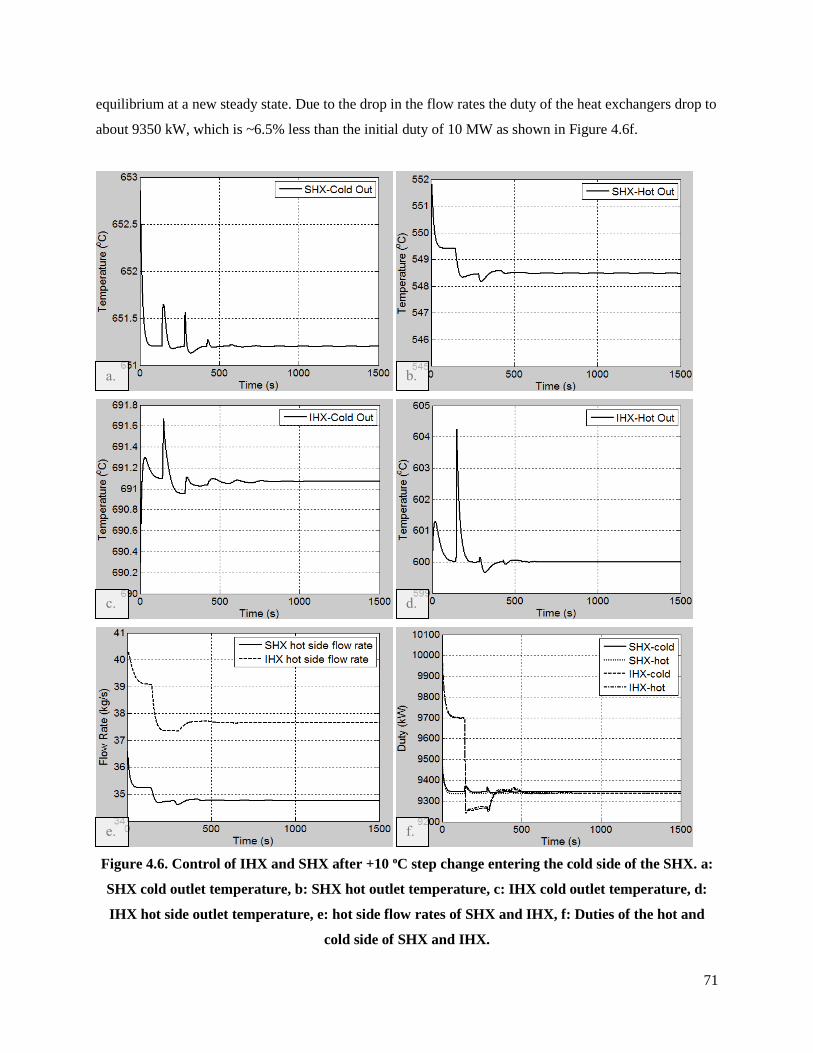
71
equilibrium at a new steady state. Due to the drop in the flow rates the duty of the heat exchangers drop to
about 9350 kW, which is ~6.5% less than the initial duty of 10 MW as shown in Figure 4.6f.
Figure 4.6. Control of IHX and SHX after +10 oC step change entering the cold side of the SHX. a:
SHX cold outlet temperature, b: SHX hot outlet temperature, c: IHX cold outlet temperature, d:
IHX hot side outlet temperature, e: hot side flow rates of SHX and IHX, f: Duties of the hot and
cold side of SHX and IHX.
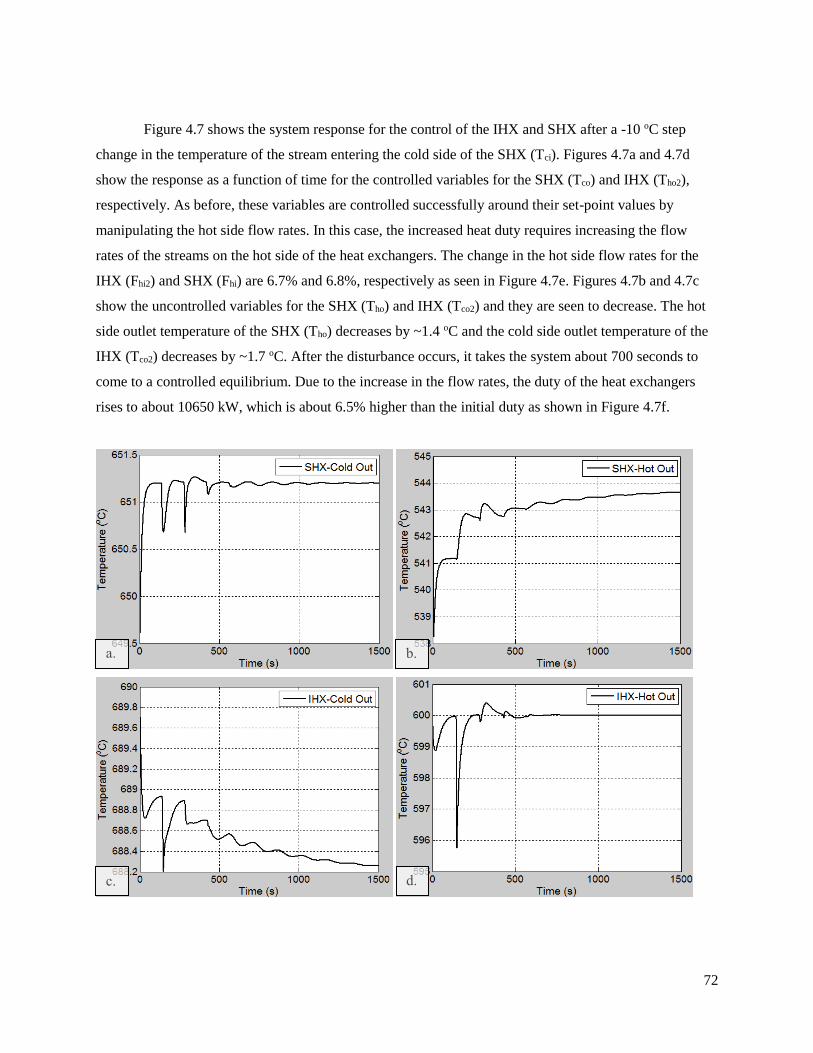
72
Figure 4.7 shows the system response for the control of the IHX and SHX after a -10 oC step
change in the temperature of the stream entering the cold side of the SHX (Tci). Figures 4.7a and 4.7d
show the response as a function of time for the controlled variables for the SHX (Tco) and IHX (Tho2),
respectively. As before, these variables are controlled successfully around their set-point values by
manipulating the hot side flow rates. In this case, the increased heat duty requires increasing the flow
rates of the streams on the hot side of the heat exchangers. The change in the hot side flow rates for the
IHX (Fhi2) and SHX (Fhi) are 6.7% and 6.8%, respectively as seen in Figure 4.7e. Figures 4.7b and 4.7c
show the uncontrolled variables for the SHX (Tho) and IHX (Tco2) and they are seen to decrease. The hot
side outlet temperature of the SHX (Tho) decreases by ~1.4 oC and the cold side outlet temperature of the
IHX (Tco2) decreases by ~1.7 oC. After the disturbance occurs, it takes the system about 700 seconds to
come to a controlled equilibrium. Due to the increase in the flow rates, the duty of the heat exchangers
rises to about 10650 kW, which is about 6.5% higher than the initial duty as shown in Figure 4.7f.
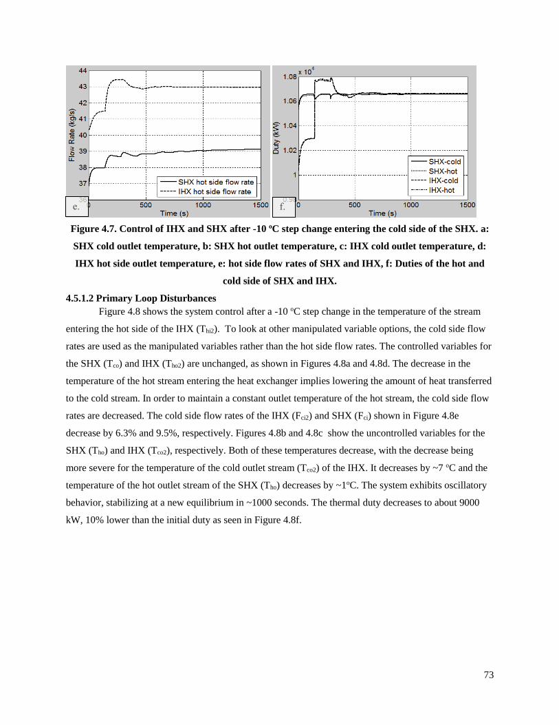
73
Figure 4.7. Control of IHX and SHX after -10 oC step change entering the cold side of the SHX. a:
SHX cold outlet temperature, b: SHX hot outlet temperature, c: IHX cold outlet temperature, d:
IHX hot side outlet temperature, e: hot side flow rates of SHX and IHX, f: Duties of the hot and
cold side of SHX and IHX.
4.5.1.2 Primary Loop Disturbances
Figure 4.8 shows the system control after a -10 oC step change in the temperature of the stream
entering the hot side of the IHX (Thi2). To look at other manipulated variable options, the cold side flow
rates are used as the manipulated variables rather than the hot side flow rates. The controlled variables for
the SHX (Tco) and IHX (Tho2) are unchanged, as shown in Figures 4.8a and 4.8d. The decrease in the
temperature of the hot stream entering the heat exchanger implies lowering the amount of heat transferred
to the cold stream. In order to maintain a constant outlet temperature of the hot stream, the cold side flow
rates are decreased. The cold side flow rates of the IHX (Fci2) and SHX (Fci) shown in Figure 4.8e
decrease by 6.3% and 9.5%, respectively. Figures 4.8b and 4.8c show the uncontrolled variables for the
SHX (Tho) and IHX (Tco2), respectively. Both of these temperatures decrease, with the decrease being
more severe for the temperature of the cold outlet stream (Tco2) of the IHX. It decreases by ~7 oC and the
temperature of the hot outlet stream of the SHX (Tho) decreases by ~1oC. The system exhibits oscillatory
behavior, stabilizing at a new equilibrium in ~1000 seconds. The thermal duty decreases to about 9000
kW, 10% lower than the initial duty as seen in Figure 4.8f.
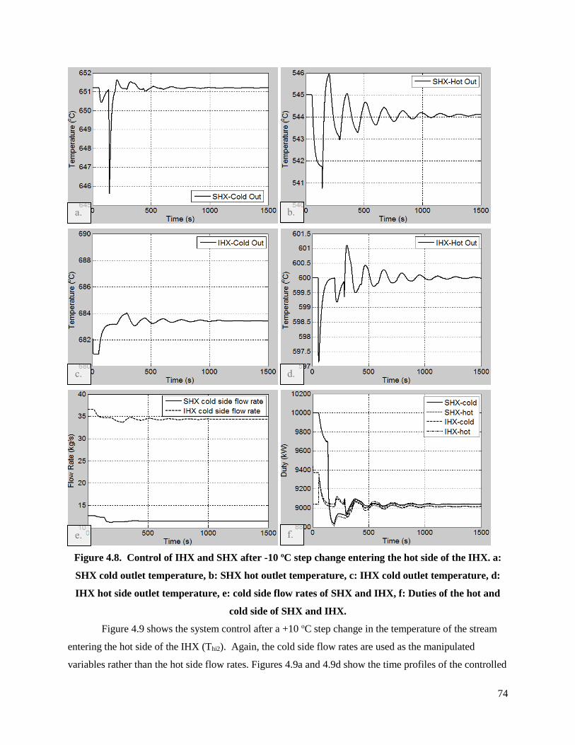
74
Figure 4.8. Control of IHX and SHX after -10 oC step change entering the hot side of the IHX. a:
SHX cold outlet temperature, b: SHX hot outlet temperature, c: IHX cold outlet temperature, d:
IHX hot side outlet temperature, e: cold side flow rates of SHX and IHX, f: Duties of the hot and
cold side of SHX and IHX.
Figure 4.9 shows the system control after a +10 oC step change in the temperature of the stream
entering the hot side of the IHX (Thi2). Again, the cold side flow rates are used as the manipulated
variables rather than the hot side flow rates. Figures 4.9a and 4.9d show the time profiles of the controlled
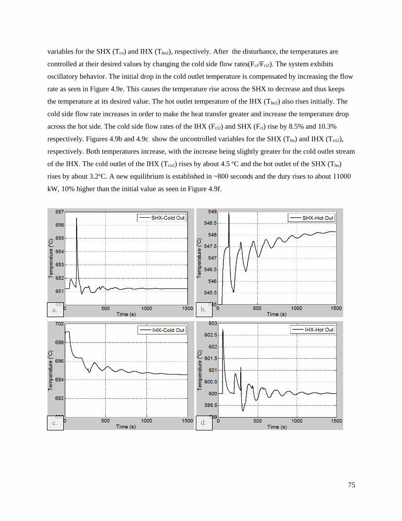
75
variables for the SHX (Tco) and IHX (Tho2), respectively. After the disturbance, the temperatures are
controlled at their desired values by changing the cold side flow rates(Fci/Fci2). The system exhibits
oscillatory behavior. The initial drop in the cold outlet temperature is compensated by increasing the flow
rate as seen in Figure 4.9e. This causes the temperature rise across the SHX to decrease and thus keeps
the temperature at its desired value. The hot outlet temperature of the IHX (Tho2) also rises initially. The
cold side flow rate increases in order to make the heat transfer greater and increase the temperature drop
across the hot side. The cold side flow rates of the IHX (Fci2) and SHX (Fci) rise by 8.5% and 10.3%
respectively. Figures 4.9b and 4.9c show the uncontrolled variables for the SHX (Tho) and IHX (Tco2),
respectively. Both temperatures increase, with the increase being slightly greater for the cold outlet stream
of the IHX. The cold outlet of the IHX (Tco2) rises by about 4.5 oC and the hot outlet of the SHX (Tho)
rises by about 3.2oC. A new equilibrium is established in ~800 seconds and the duty rises to about 11000
kW, 10% higher than the initial value as seen in Figure 4.9f.
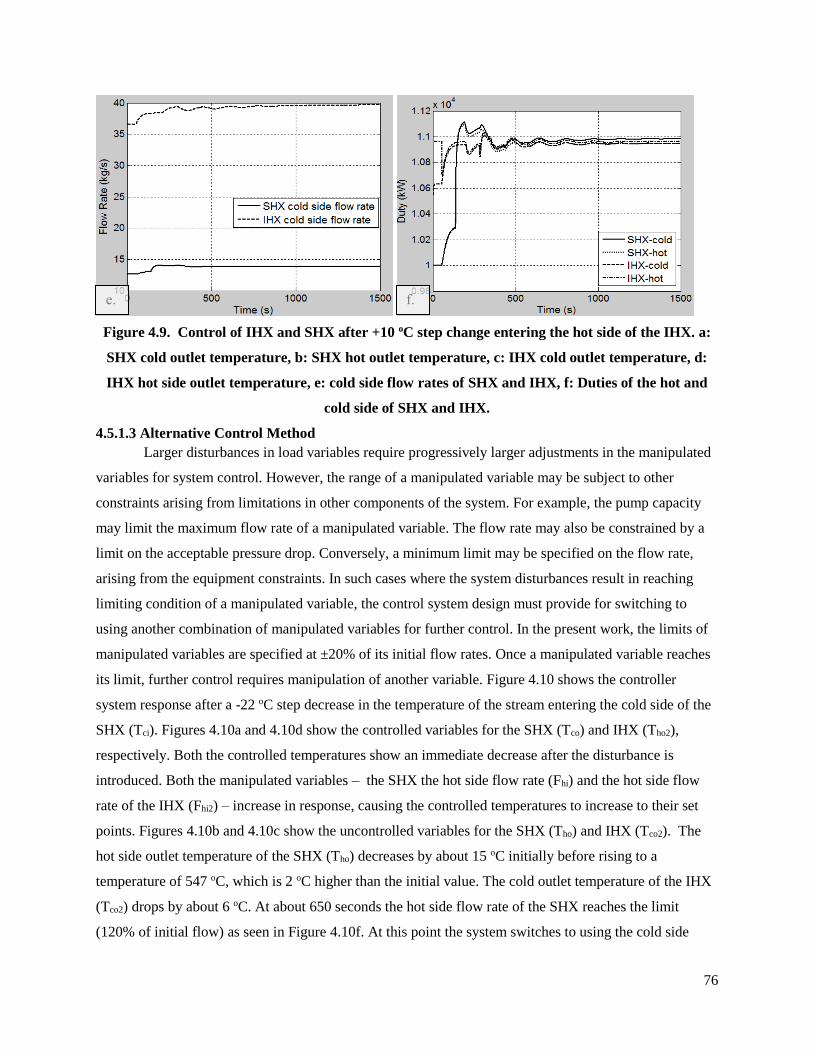
76
Figure 4.9. Control of IHX and SHX after +10 oC step change entering the hot side of the IHX. a:
SHX cold outlet temperature, b: SHX hot outlet temperature, c: IHX cold outlet temperature, d:
IHX hot side outlet temperature, e: cold side flow rates of SHX and IHX, f: Duties of the hot and
cold side of SHX and IHX.
4.5.1.3 Alternative Control Method
Larger disturbances in load variables require progressively larger adjustments in the manipulated
variables for system control. However, the range of a manipulated variable may be subject to other
constraints arising from limitations in other components of the system. For example, the pump capacity
may limit the maximum flow rate of a manipulated variable. The flow rate may also be constrained by a
limit on the acceptable pressure drop. Conversely, a minimum limit may be specified on the flow rate,
arising from the equipment constraints. In such cases where the system disturbances result in reaching
limiting condition of a manipulated variable, the control system design must provide for switching to
using another combination of manipulated variables for further control. In the present work, the limits of
manipulated variables are specified at ±20% of its initial flow rates. Once a manipulated variable reaches
its limit, further control requires manipulation of another variable. Figure 4.10 shows the controller
system response after a -22 oC step decrease in the temperature of the stream entering the cold side of the
SHX (Tci). Figures 4.10a and 4.10d show the controlled variables for the SHX (Tco) and IHX (Tho2),
respectively. Both the controlled temperatures show an immediate decrease after the disturbance is
introduced. Both the manipulated variables – the SHX the hot side flow rate (Fhi) and the hot side flow
rate of the IHX (Fhi2) – increase in response, causing the controlled temperatures to increase to their set
points. Figures 4.10b and 4.10c show the uncontrolled variables for the SHX (Tho) and IHX (Tco2). The
hot side outlet temperature of the SHX (Tho) decreases by about 15 oC initially before rising to a
temperature of 547 oC, which is 2 oC higher than the initial value. The cold outlet temperature of the IHX
(Tco2) drops by about 6 oC. At about 650 seconds the hot side flow rate of the SHX reaches the limit
(120% of initial flow) as seen in Figure 4.10f. At this point the system switches to using the cold side
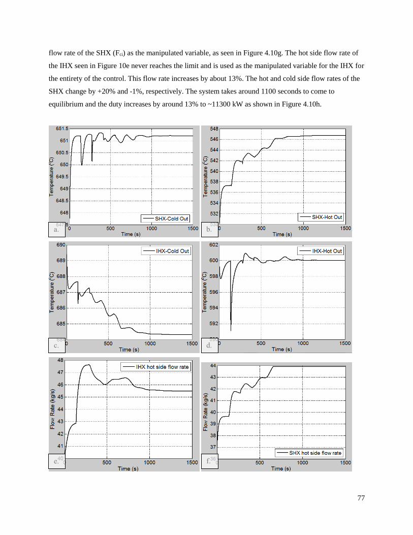
77
flow rate of the SHX (Fci) as the manipulated variable, as seen in Figure 4.10g. The hot side flow rate of
the IHX seen in Figure 10e never reaches the limit and is used as the manipulated variable for the IHX for
the entirety of the control. This flow rate increases by about 13%. The hot and cold side flow rates of the
SHX change by +20% and -1%, respectively. The system takes around 1100 seconds to come to
equilibrium and the duty increases by around 13% to ~11300 kW as shown in Figure 4.10h.
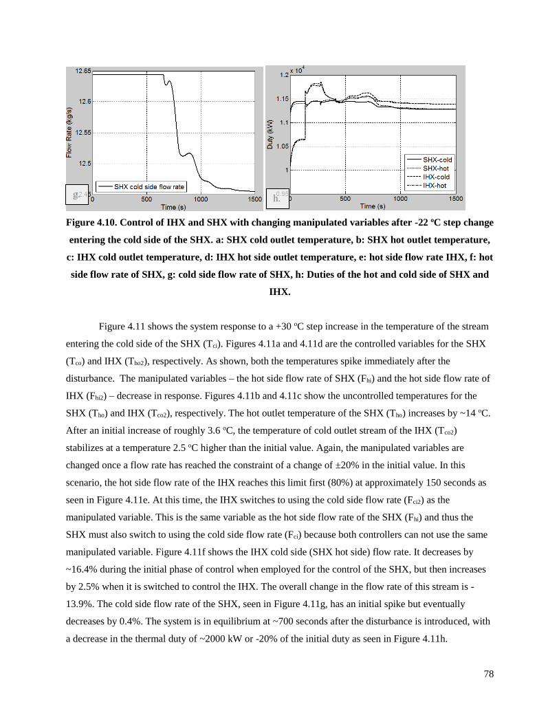
78
Figure 4.10. Control of IHX and SHX with changing manipulated variables after -22 oC step change
entering the cold side of the SHX. a: SHX cold outlet temperature, b: SHX hot outlet temperature,
c: IHX cold outlet temperature, d: IHX hot side outlet temperature, e: hot side flow rate IHX, f: hot
side flow rate of SHX, g: cold side flow rate of SHX, h: Duties of the hot and cold side of SHX and
IHX.
Figure 4.11 shows the system response to a +30 oC step increase in the temperature of the stream
entering the cold side of the SHX (Tci). Figures 4.11a and 4.11d are the controlled variables for the SHX
(Tco) and IHX (Tho2), respectively. As shown, both the temperatures spike immediately after the
disturbance. The manipulated variables – the hot side flow rate of SHX (Fhi) and the hot side flow rate of
IHX (Fhi2) – decrease in response. Figures 4.11b and 4.11c show the uncontrolled temperatures for the
SHX (Tho) and IHX (Tco2), respectively. The hot outlet temperature of the SHX (Tho) increases by ~14 oC.
After an initial increase of roughly 3.6 oC, the temperature of cold outlet stream of the IHX (Tco2)
stabilizes at a temperature 2.5 oC higher than the initial value. Again, the manipulated variables are
changed once a flow rate has reached the constraint of a change of ±20% in the initial value. In this
scenario, the hot side flow rate of the IHX reaches this limit first (80%) at approximately 150 seconds as
seen in Figure 4.11e. At this time, the IHX switches to using the cold side flow rate (Fci2) as the
manipulated variable. This is the same variable as the hot side flow rate of the SHX (Fhi) and thus the
SHX must also switch to using the cold side flow rate (Fci) because both controllers can not use the same
manipulated variable. Figure 4.11f shows the IHX cold side (SHX hot side) flow rate. It decreases by
~16.4% during the initial phase of control when employed for the control of the SHX, but then increases
by 2.5% when it is switched to control the IHX. The overall change in the flow rate of this stream is -
13.9%. The cold side flow rate of the SHX, seen in Figure 4.11g, has an initial spike but eventually
decreases by 0.4%. The system is in equilibrium at ~700 seconds after the disturbance is introduced, with
a decrease in the thermal duty of ~2000 kW or -20% of the initial duty as seen in Figure 4.11h.
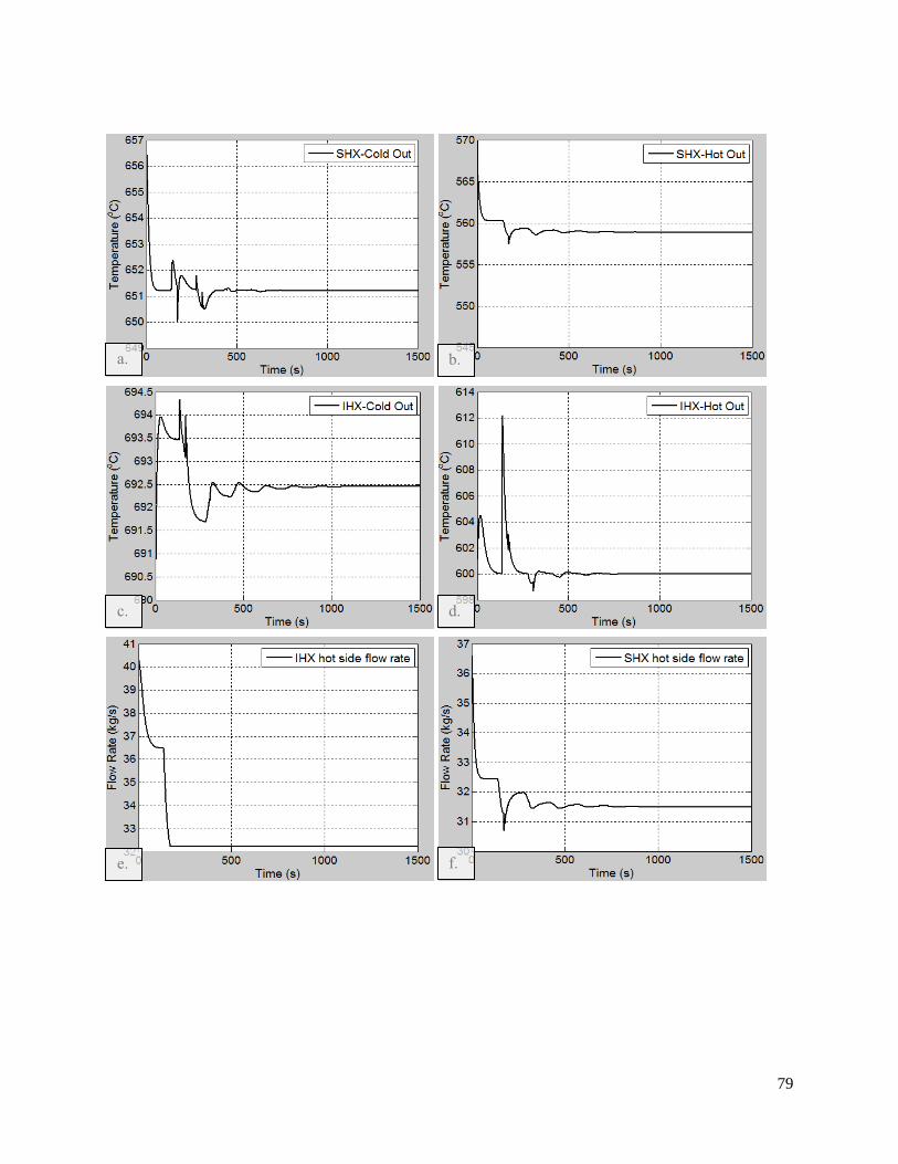
79
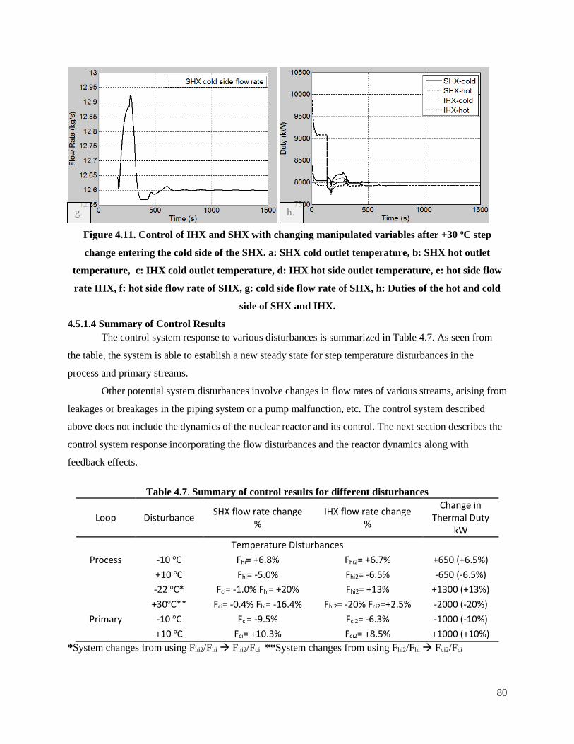
80
Figure 4.11. Control of IHX and SHX with changing manipulated variables after +30 oC step
change entering the cold side of the SHX. a: SHX cold outlet temperature, b: SHX hot outlet
temperature, c: IHX cold outlet temperature, d: IHX hot side outlet temperature, e: hot side flow
rate IHX, f: hot side flow rate of SHX, g: cold side flow rate of SHX, h: Duties of the hot and cold
side of SHX and IHX.
4.5.1.4 Summary of Control Results
The control system response to various disturbances is summarized in Table 4.7. As seen from
the table, the system is able to establish a new steady state for step temperature disturbances in the
process and primary streams.
Other potential system disturbances involve changes in flow rates of various streams, arising from
leakages or breakages in the piping system or a pump malfunction, etc. The control system described
above does not include the dynamics of the nuclear reactor and its control. The next section describes the
control system response incorporating the flow disturbances and the reactor dynamics along with
feedback effects.
Table 4.7. Summary of control results for different disturbances
Loop Disturbance SHX flow rate change
% IHX flow rate change
%
Change in Thermal Duty
kW
Temperature Disturbances
Process -10 oC Fhi= +6.8% Fhi2= +6.7% +650 (+6.5%) +10 oC Fhi= -5.0% Fhi2= -6.5% -650 (-6.5%)
-22 oC* Fci= -1.0% Fhi= +20% Fhi2= +13% +1300 (+13%)
+30oC** Fci= -0.4% Fhi= -16.4% Fhi2= -20% Fci2=+2.5% -2000 (-20%)
Primary -10 oC Fci= -9.5% Fci2= -6.3% -1000 (-10%) +10 oC Fci= +10.3% Fci2= +8.5% +1000 (+10%)
*System changes from using Fhi2/Fhi Fhi2/Fci **System changes from using Fhi2/Fhi Fci2/Fci
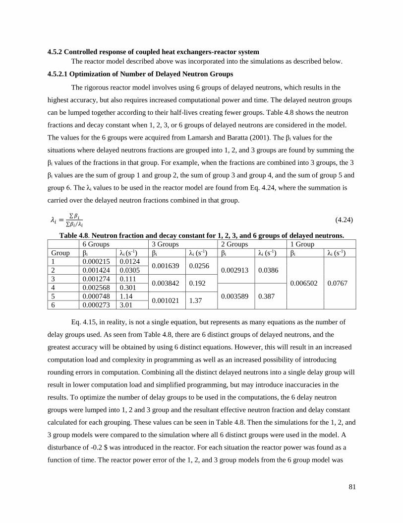
81
4.5.2 Controlled response of coupled heat exchangers-reactor system
The reactor model described above was incorporated into the simulations as described below.
4.5.2.1 Optimization of Number of Delayed Neutron Groups
The rigorous reactor model involves using 6 groups of delayed neutrons, which results in the
highest accuracy, but also requires increased computational power and time. The delayed neutron groups
can be lumped together according to their half-lives creating fewer groups. Table 4.8 shows the neutron
fractions and decay constant when 1, 2, 3, or 6 groups of delayed neutrons are considered in the model.
The values for the 6 groups were acquired from Lamarsh and Baratta (2001). The βi values for the
situations where delayed neutrons fractions are grouped into 1, 2, and 3 groups are found by summing the
βi values of the fractions in that group. For example, when the fractions are combined into 3 groups, the 3
βi values are the sum of group 1 and group 2, the sum of group 3 and group 4, and the sum of group 5 and
group 6. The λi values to be used in the reactor model are found from Eq. 4.24, where the summation is
carried over the delayed neutron fractions combined in that group.
𝜆𝑖 =∑ 𝛽𝑖
∑𝛽𝑖 𝜆𝑖⁄ (4.24)
Table 4.8. Neutron fraction and decay constant for 1, 2, 3, and 6 groups of delayed neutrons.
6 Groups 3 Groups 2 Groups 1 Group
Group βi λi (s-1) βi λi (s-1) βi λi (s-1) βi λi (s-1)
1 0.000215 0.0124 0.001639 0.0256
0.002913 0.0386
0.006502 0.0767
2 0.001424 0.0305
3 0.001274 0.111 0.003842 0.192
4 0.002568 0.301
0.003589 0.387 5 0.000748 1.14 0.001021 1.37
6 0.000273 3.01
Eq. 4.15, in reality, is not a single equation, but represents as many equations as the number of
delay groups used. As seen from Table 4.8, there are 6 distinct groups of delayed neutrons, and the
greatest accuracy will be obtained by using 6 distinct equations. However, this will result in an increased
computation load and complexity in programming as well as an increased possibility of introducing
rounding errors in computation. Combining all the distinct delayed neutrons into a single delay group will
result in lower computation load and simplified programming, but may introduce inaccuracies in the
results. To optimize the number of delay groups to be used in the computations, the 6 delay neutron
groups were lumped into 1, 2 and 3 group and the resultant effective neutron fraction and delay constant
calculated for each grouping. These values can be seen in Table 4.8. Then the simulations for the 1, 2, and
3 group models were compared to the simulation where all 6 distinct groups were used in the model. A
disturbance of -0.2 $ was introduced in the reactor. For each situation the reactor power was found as a
function of time. The reactor power error of the 1, 2, and 3 group models from the 6 group model was
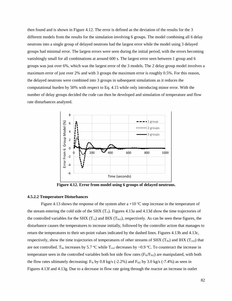
82
then found and is shown in Figure 4.12. The error is defined as the deviation of the results for the 3
different models from the results for the simulation involving 6 groups. The model combining all 6 delay
neutrons into a single group of delayed neutrons had the largest error while the model using 3 delayed
groups had minimal error. The largest errors were seen during the initial period, with the errors becoming
vanishingly small for all combinations at around 600 s. The largest error seen between 1 group and 6
groups was just over 6%, which was the largest error of the 3 models. The 2 delay group model involves a
maximum error of just over 2% and with 3 groups the maximum error is roughly 0.5%. For this reason,
the delayed neutrons were combined into 3 groups in subsequent simulations as it reduces the
computational burden by 50% with respect to Eq. 4.15 while only introducing minor error. With the
number of delay groups decided the code can then be developed and simulation of temperature and flow
rate disturbances analyzed.
Figure 4.12. Error from model using 6 groups of delayed neutrons.
4.5.2.2 Temperature Disturbances
Figure 4.13 shows the response of the system after a +10 oC step increase in the temperature of
the stream entering the cold side of the SHX (Tci). Figures 4.13a and 4.13d show the time trajectories of
the controlled variables for the SHX (Tco) and IHX (Tho2), respectively. As can be seen these figures, the
disturbance causes the temperatures to increase initially, followed by the controller action that manages to
return the temperatures to their set-point values indicated by the dashed lines. Figures 4.13b and 4.13c,
respectively, show the time trajectories of temperatures of other streams of SHX (Tho) and IHX (Tco2) that
are not controlled. Tho increases by 5.7 oC while Tco2 decreases by ~0.9 oC. To counteract the increase in
temperature seen in the controlled variables both hot side flow rates (Fhi/Fhi2) are manipulated, with both
the flow rates ultimately decreasing: Fhi by 0.8 kg/s (-2.2%) and Fhi2 by 3.0 kg/s (-7.4%) as seen in
Figures 4.13f and 4.13g. Due to a decrease in flow rate going through the reactor an increase in outlet
-6
-4
-2
0
2
4
6
8
0 200 400 600 800 1000
Erro
r Fr
om
6 G
rou
p M
od
el (
%)
Time (seconds)
1 group
2 groups
3 groups
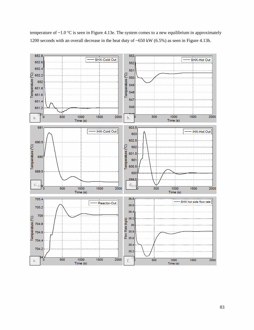
83
temperature of ~1.0 oC is seen in Figure 4.13e. The system comes to a new equilibrium in approximately
1200 seconds with an overall decrease in the heat duty of ~650 kW (6.5%) as seen in Figure 4.13h.
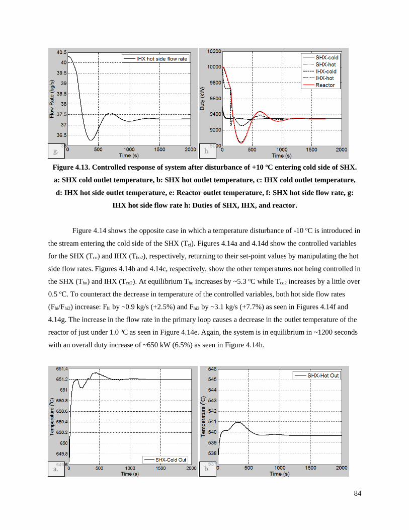
84
Figure 4.13. Controlled response of system after disturbance of +10 oC entering cold side of SHX.
a: SHX cold outlet temperature, b: SHX hot outlet temperature, c: IHX cold outlet temperature,
d: IHX hot side outlet temperature, e: Reactor outlet temperature, f: SHX hot side flow rate, g:
IHX hot side flow rate h: Duties of SHX, IHX, and reactor.
Figure 4.14 shows the opposite case in which a temperature disturbance of -10 oC is introduced in
the stream entering the cold side of the SHX (Tci). Figures 4.14a and 4.14d show the controlled variables
for the SHX (Tco) and IHX (Tho2), respectively, returning to their set-point values by manipulating the hot
side flow rates. Figures 4.14b and 4.14c, respectively, show the other temperatures not being controlled in
the SHX (Tho) and IHX (Tco2). At equilibrium Tho increases by ~5.3 oC while Tco2 increases by a little over
0.5 oC. To counteract the decrease in temperature of the controlled variables, both hot side flow rates
(Fhi/Fhi2) increase: Fhi by ~0.9 kg/s (+2.5%) and Fhi2 by ~3.1 kg/s (+7.7%) as seen in Figures 4.14f and
4.14g. The increase in the flow rate in the primary loop causes a decrease in the outlet temperature of the
reactor of just under 1.0 oC as seen in Figure 4.14e. Again, the system is in equilibrium in ~1200 seconds
with an overall duty increase of ~650 kW (6.5%) as seen in Figure 4.14h.
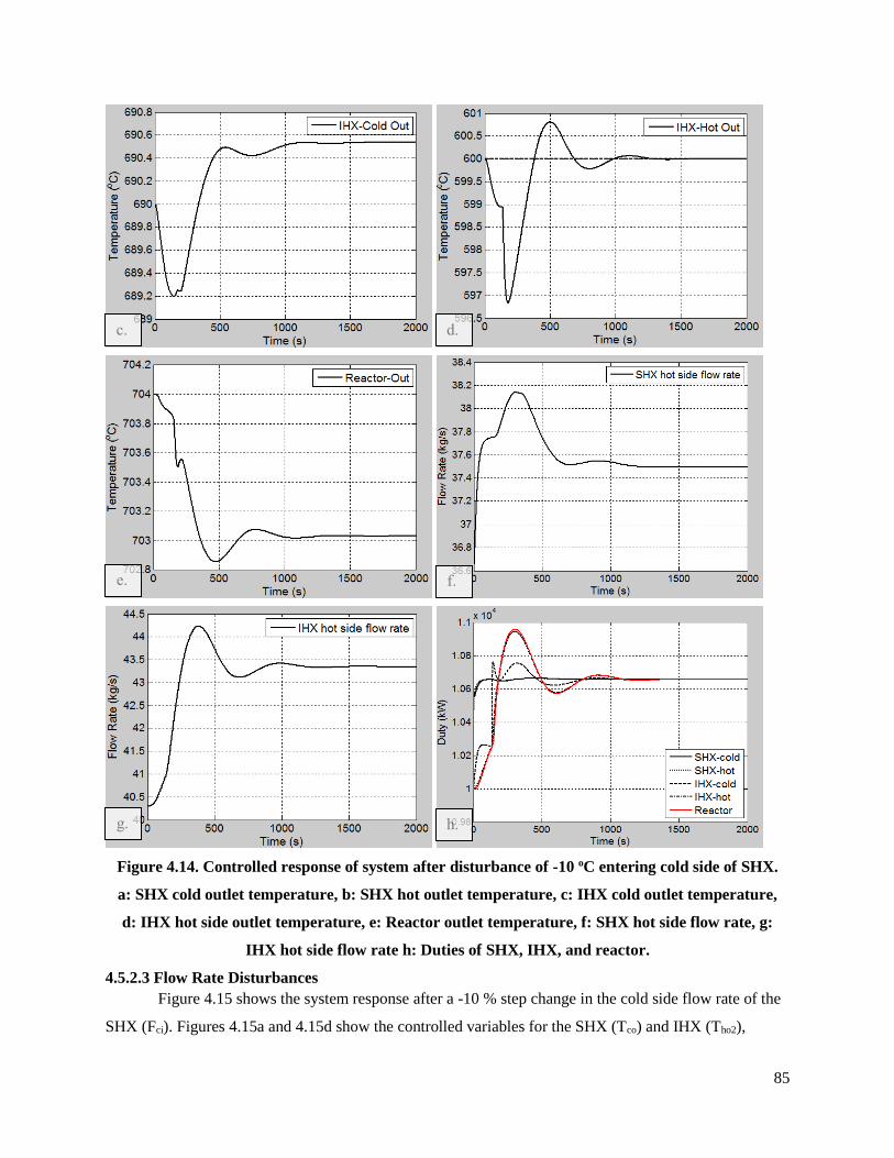
85
Figure 4.14. Controlled response of system after disturbance of -10 oC entering cold side of SHX.
a: SHX cold outlet temperature, b: SHX hot outlet temperature, c: IHX cold outlet temperature,
d: IHX hot side outlet temperature, e: Reactor outlet temperature, f: SHX hot side flow rate, g:
IHX hot side flow rate h: Duties of SHX, IHX, and reactor.
4.5.2.3 Flow Rate Disturbances
Figure 4.15 shows the system response after a -10 % step change in the cold side flow rate of the
SHX (Fci). Figures 4.15a and 4.15d show the controlled variables for the SHX (Tco) and IHX (Tho2),
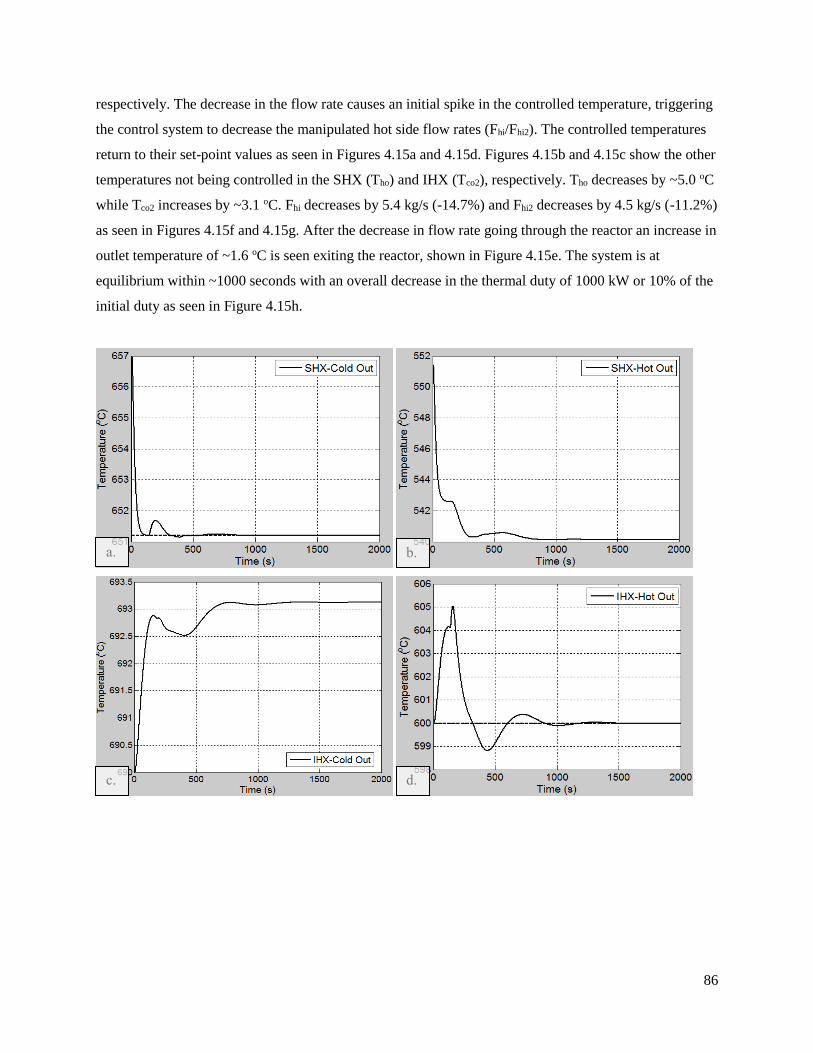
86
respectively. The decrease in the flow rate causes an initial spike in the controlled temperature, triggering
the control system to decrease the manipulated hot side flow rates (Fhi/Fhi2). The controlled temperatures
return to their set-point values as seen in Figures 4.15a and 4.15d. Figures 4.15b and 4.15c show the other
temperatures not being controlled in the SHX (Tho) and IHX (Tco2), respectively. Tho decreases by ~5.0 oC
while Tco2 increases by ~3.1 oC. Fhi decreases by 5.4 kg/s (-14.7%) and Fhi2 decreases by 4.5 kg/s (-11.2%)
as seen in Figures 4.15f and 4.15g. After the decrease in flow rate going through the reactor an increase in
outlet temperature of ~1.6 oC is seen exiting the reactor, shown in Figure 4.15e. The system is at
equilibrium within ~1000 seconds with an overall decrease in the thermal duty of 1000 kW or 10% of the
initial duty as seen in Figure 4.15h.
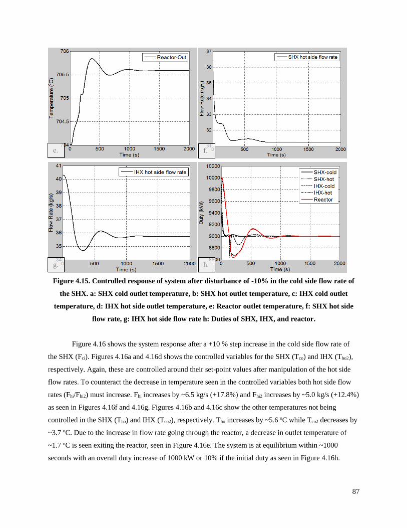
87
Figure 4.15. Controlled response of system after disturbance of -10% in the cold side flow rate of
the SHX. a: SHX cold outlet temperature, b: SHX hot outlet temperature, c: IHX cold outlet
temperature, d: IHX hot side outlet temperature, e: Reactor outlet temperature, f: SHX hot side
flow rate, g: IHX hot side flow rate h: Duties of SHX, IHX, and reactor.
Figure 4.16 shows the system response after a +10 % step increase in the cold side flow rate of
the SHX (Fci). Figures 4.16a and 4.16d shows the controlled variables for the SHX (Tco) and IHX (Tho2),
respectively. Again, these are controlled around their set-point values after manipulation of the hot side
flow rates. To counteract the decrease in temperature seen in the controlled variables both hot side flow
rates (Fhi/Fhi2) must increase. Fhi increases by ~6.5 kg/s (+17.8%) and Fhi2 increases by ~5.0 kg/s (+12.4%)
as seen in Figures 4.16f and 4.16g. Figures 4.16b and 4.16c show the other temperatures not being
controlled in the SHX (Tho) and IHX (Tco2), respectively. Tho increases by ~5.6 oC while Tco2 decreases by
~3.7 oC. Due to the increase in flow rate going through the reactor, a decrease in outlet temperature of
~1.7 oC is seen exiting the reactor, seen in Figure 4.16e. The system is at equilibrium within ~1000
seconds with an overall duty increase of 1000 kW or 10% if the initial duty as seen in Figure 4.16h.
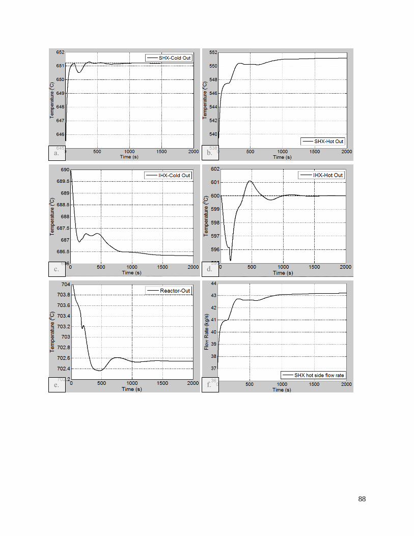
88
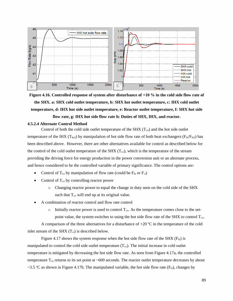
89
Figure 4.16. Controlled response of system after disturbance of +10 % in the cold side flow rate of
the SHX. a: SHX cold outlet temperature, b: SHX hot outlet temperature, c: IHX cold outlet
temperature, d: IHX hot side outlet temperature, e: Reactor outlet temperature, f: SHX hot side
flow rate, g: IHX hot side flow rate h: Duties of SHX, IHX, and reactor.
4.5.2.4 Alternate Control Method
Control of both the cold side outlet temperature of the SHX (Tco) and the hot side outlet
temperature of the IHX (Tho2) by manipulation of hot side flow rate of both heat exchangers (Fhi/Fhi2) has
been described above. However, there are other alternatives available for control as described below for
the control of the cold outlet temperature of the SHX (Tco), which is the temperature of the stream
providing the driving force for energy production in the power conversion unit or an alternate process,
and hence considered to be the controlled variable of primary significance. The control options are:
Control of Tco by manipulation of flow rate (could be Fhi or Fci)
Control of Tco by controlling reactor power
o Changing reactor power to equal the change in duty seen on the cold side of the SHX
such that Tco will end up at its original value.
A combination of reactor control and flow rate control
o Initially reactor power is used to control Tco. As the temperature comes close to the set-
point value, the system switches to using the hot side flow rate of the SHX to control Tco.
A comparison of the three alternatives for a disturbance of +20 oC in the temperature of the cold
inlet stream of the SHX (Tci) is described below.
Figure 4.17 shows the system response when the hot side flow rate of the SHX (Fhi) is
manipulated to control the cold side outlet temperature (Tco). The initial increase in cold outlet
temperature is mitigated by decreasing the hot side flow rate. As seen from Figure 4.17a, the controlled
temperature Tco returns to its set point at ~600 seconds. The reactor outlet temperature decreases by about
~3.5 oC as shown in Figure 4.17b. The manipulated variable, the hot side flow rate (Fhi), changes by
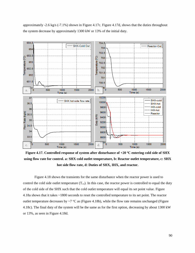
90
approximately -2.6 kg/s (-7.1%) shown in Figure 4.17c. Figure 4.17d, shows that the duties throughout
the system decrease by approximately 1300 kW or 13% of the initial duty.
Figure 4.17. Controlled response of system after disturbance of +20 oC entering cold side of SHX
using flow rate for control. a: SHX cold outlet temperature, b: Reactor outlet temperature, c: SHX
hot side flow rate, d: Duties of SHX, IHX, and reactor.
Figure 4.18 shows the transients for the same disturbance when the reactor power is used to
control the cold side outlet temperature (Tco). In this case, the reactor power is controlled to equal the duty
of the cold side of the SHX such that the cold outlet temperature will equal its set point value. Figure
4.18a shows that it takes ~1800 seconds to reset the controlled temperature to its set point. The reactor
outlet temperature decreases by ~7 oC as (Figure 4.18b), while the flow rate remains unchanged (Figure
4.18c). The final duty of the system will be the same as for the first option, decreasing by about 1300 kW
or 13%, as seen in Figure 4.18d.
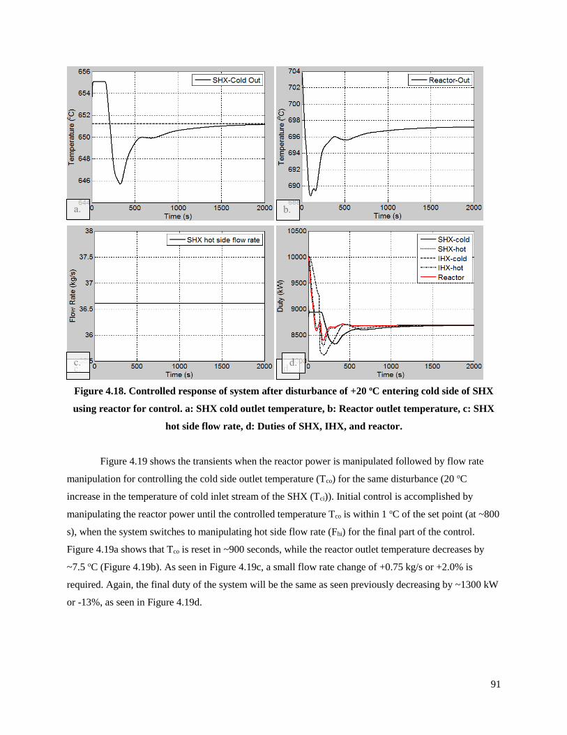
91
Figure 4.18. Controlled response of system after disturbance of +20 oC entering cold side of SHX
using reactor for control. a: SHX cold outlet temperature, b: Reactor outlet temperature, c: SHX
hot side flow rate, d: Duties of SHX, IHX, and reactor.
Figure 4.19 shows the transients when the reactor power is manipulated followed by flow rate
manipulation for controlling the cold side outlet temperature (Tco) for the same disturbance (20 oC
increase in the temperature of cold inlet stream of the SHX (Tci)). Initial control is accomplished by
manipulating the reactor power until the controlled temperature Tco is within 1 oC of the set point (at ~800
s), when the system switches to manipulating hot side flow rate (Fhi) for the final part of the control.
Figure 4.19a shows that Tco is reset in ~900 seconds, while the reactor outlet temperature decreases by
~7.5 oC (Figure 4.19b). As seen in Figure 4.19c, a small flow rate change of +0.75 kg/s or +2.0% is
required. Again, the final duty of the system will be the same as seen previously decreasing by ~1300 kW
or -13%, as seen in Figure 4.19d.
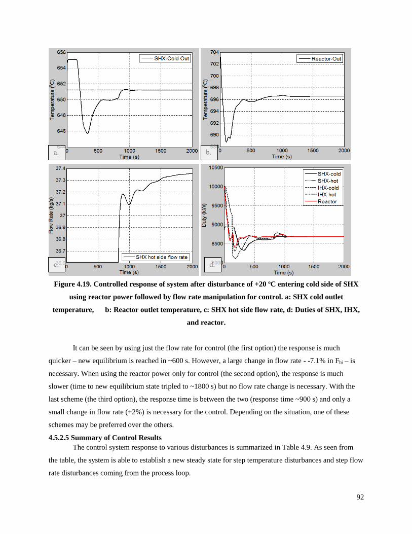
92
Figure 4.19. Controlled response of system after disturbance of +20 oC entering cold side of SHX
using reactor power followed by flow rate manipulation for control. a: SHX cold outlet
temperature, b: Reactor outlet temperature, c: SHX hot side flow rate, d: Duties of SHX, IHX,
and reactor.
It can be seen by using just the flow rate for control (the first option) the response is much
quicker – new equilibrium is reached in ~600 s. However, a large change in flow rate - -7.1% in Fhi – is
necessary. When using the reactor power only for control (the second option), the response is much
slower (time to new equilibrium state tripled to ~1800 s) but no flow rate change is necessary. With the
last scheme (the third option), the response time is between the two (response time ~900 s) and only a
small change in flow rate (+2%) is necessary for the control. Depending on the situation, one of these
schemes may be preferred over the others.
4.5.2.5 Summary of Control Results
The control system response to various disturbances is summarized in Table 4.9. As seen from
the table, the system is able to establish a new steady state for step temperature disturbances and step flow
rate disturbances coming from the process loop.
93
Table 4.9. Summary of control results for different disturbances with reactor.
Loop Disturbance SHX flow rate change
% IHX flow rate change
%
Change in Thermal Duty
kW
Temperature Disturbances
Process -10 oC Fhi= +2.5% Fhi2= +7.7% +650 (+6.5%) +10 oC Fhi= -2.2% Fhi2= -7.4% -650 (-6.5%)
Flow Rate Disturbances
-10% Fc Fhi= -14.8% Fhi2= -11.2% -1000 (-10%)
+10% Fc Fhi= +17.8% Fhi2= +12.4% +1000 (+10%)
It can be seen that flow rate disturbances require a larger manipulation of the hot side flow rates
than temperature disturbances for control. Normalizing the disturbances on the basis of the disturbance in
the thermal duty indicates similar level of changes in the hot side flow rate of the IHX (Fhi2, column 4) for
both flow rate and temperature disturbances. However, for the SHX, a much larger change in the hot side
flow rate (Fhi, column 3) is necessary for flow rate disturbances than temperature disturbances. Apart from
the magnitude of changes in flow rate, another factor of importance is the time period for which the cold
side outlet temperature of the SHX (Tco) is not around its set point value. The simulation results show that
at any given time the temperature does not exceed ~±5 oC from the design value with these disturbances
due to the quick responses of the tuned PID controllers. In addition, the SHX responds quickly and within
100 seconds the temperature does not exceed 1 oC. Controlling the cold outlet temperature of the SHX
allows for the process to run at high efficiencies. The SHX is much more compact compared to IHX, thus
changes in the exchanger affect the parameters at a quicker rate. The larger IHX takes more time to react
to changes in the flow rate.
The alternate control strategy results are summarized in Table 4.10.
Table 4.10. Equilibrium time and flow rate change for alternate control strategy.
Control Option Disturbance SHX flow rate change
% Equilibrium time s
Change in Thermal Duty
kW
1 +20 oC Fhi= -7.1% 600 -1300 (-13.0%)
2 +20 oC Fhi= +0.0% 1800 -1300 (-13.0%)
3 +20 oC Fhi= +2.0% 900 -1300 (-13.0%)
As can be seen from the table, control option 3 (reactor power manipulation followed by flow rate
manipulation) response, while 50% slower than option 1 (flow rate manipulation only) is twice as fast as
the option 2 (reactor power manipulation only). Further, the flow rate change needed for option 1 is more
than 3 times as high as that for option 3. The third control method has a quick response and only a small

94
change in the flow rate is necessary. However, the controlled temperature is far from the set point value
for ~300 seconds longer than control option 1. This could have an effect on the efficiency of the process.
The process is designed to operate for a narrow range of temperature and a minimum temperature must be
present to prevent process failure. A larger disturbance may cause the temperature to dip below the
minimum value so a quick response, as seen in control option 1, may be desired. If only minimal changes
in the temperature are seen entering the process, control option 3 may be favored in order to prevent large
flow rate changes in the secondary loop.
4.5.3 Modeling and simulation of helium Brayton Cycle PCS
The control strategy and system behavior described above has a broad general applicability all
process applications including direct utilization of heat and generation of electricity. Further
investigations were conducted to determine the transient behavior of the helium Brayton cycle based PCS
shown earlier in Figure 4.2.
4.5.3.1 Steady State Design Methodolgy
The recuperator and the precooler are heat exchangers and the established design equations can be used
for their design. The design procedure for the turbine and compressor is as follows:
The turbine and compressor the outlet temperature are related to pressure ratios, inlet temperatures and
equipment efficiency by Eq. 4.25 and 4.26 (Amin and Rocco, 2006).
𝑇𝑡2 = 𝑇𝑡1 [1 − 𝜂𝑡 (1 − 𝑃𝑅𝑡
1−𝑘
𝑘 )] (4.25)
𝑇𝑐2 = 𝑇𝑐1 [1 +1
𝜂𝑐(𝑃𝑅𝑐
𝑘−1
𝑘 − 1)] (4.26)
where T is the temperature, η is the efficiency of the unit, PR is the pressure ratio (PR=P1t/P2t or
P2c/P1c), and k is the specific heat ratio which is defined as Cp/Cv. The subscripts 1, 2, t, and c stand for
inlet, outlet, turbine, and compressor, respectively. Calculation of the outlet temperature involves
determining first the pressure ratio and efficiency for each equipment. The technique presented by Wright
et al. (2006) based on the turbine and compressor performance maps shown in Fig. 4.20 and 4.21,
respectively, was used to determine these parameters. The x-axis is the specific speed (Ns) and the y-axis
specific diameter (Ds), both dimensionless parameters and are defined in Eq. 4.27 and 4.28. With a known
specific speed and specific diameter the efficiency of the turbine or compressor can be determined from
the plots.
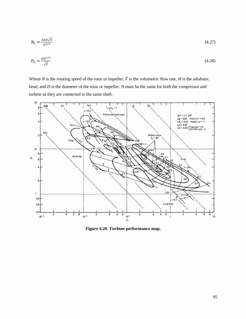
95
𝑁𝑠 =2𝜋𝑁√�̇�
𝐻3/4 (4.27)
𝐷𝑠 =𝐷𝐻1/4
√�̇� (4.28)
Where N is the rotating speed of the rotar or impeller, �̇� is the volumetric flow rate, H is the adiabatic
head, and D is the diameter of the rotar or impeller. N must be the same for both the compressor and
turbine as they are connected to the same shaft.
Figure 4.20. Turbine performance map.
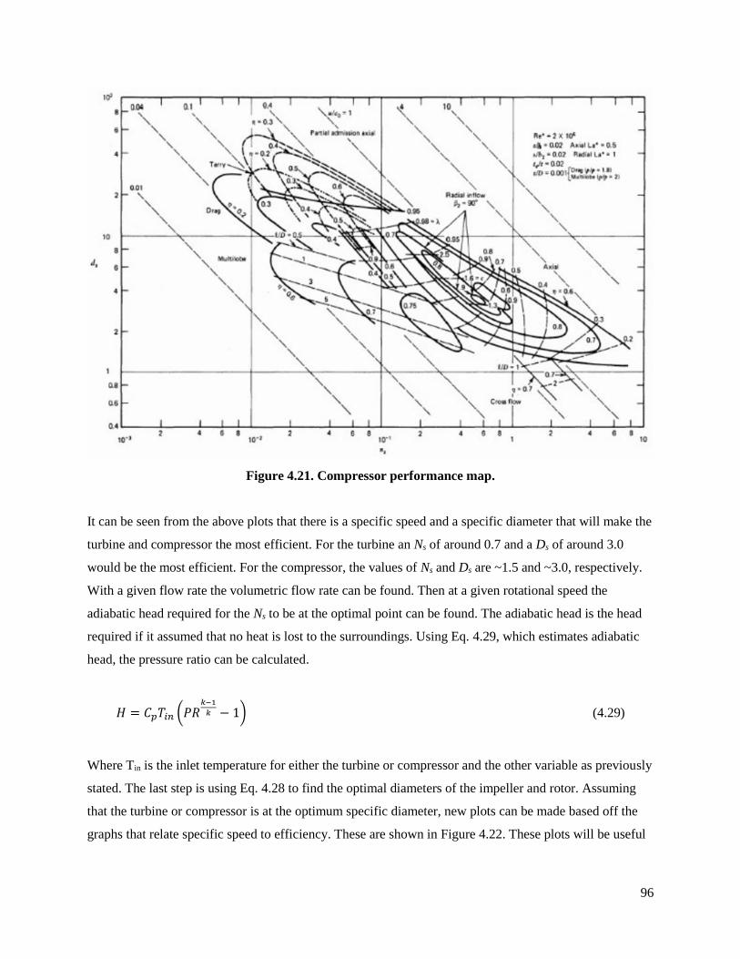
96
Figure 4.21. Compressor performance map.
It can be seen from the above plots that there is a specific speed and a specific diameter that will make the
turbine and compressor the most efficient. For the turbine an Ns of around 0.7 and a Ds of around 3.0
would be the most efficient. For the compressor, the values of Ns and Ds are ~1.5 and ~3.0, respectively.
With a given flow rate the volumetric flow rate can be found. Then at a given rotational speed the
adiabatic head required for the Ns to be at the optimal point can be found. The adiabatic head is the head
required if it assumed that no heat is lost to the surroundings. Using Eq. 4.29, which estimates adiabatic
head, the pressure ratio can be calculated.
𝐻 = 𝐶𝑝𝑇𝑖𝑛 (𝑃𝑅𝑘−1
𝑘 − 1) (4.29)
Where Tin is the inlet temperature for either the turbine or compressor and the other variable as previously
stated. The last step is using Eq. 4.28 to find the optimal diameters of the impeller and rotor. Assuming
that the turbine or compressor is at the optimum specific diameter, new plots can be made based off the
graphs that relate specific speed to efficiency. These are shown in Figure 4.22. These plots will be useful
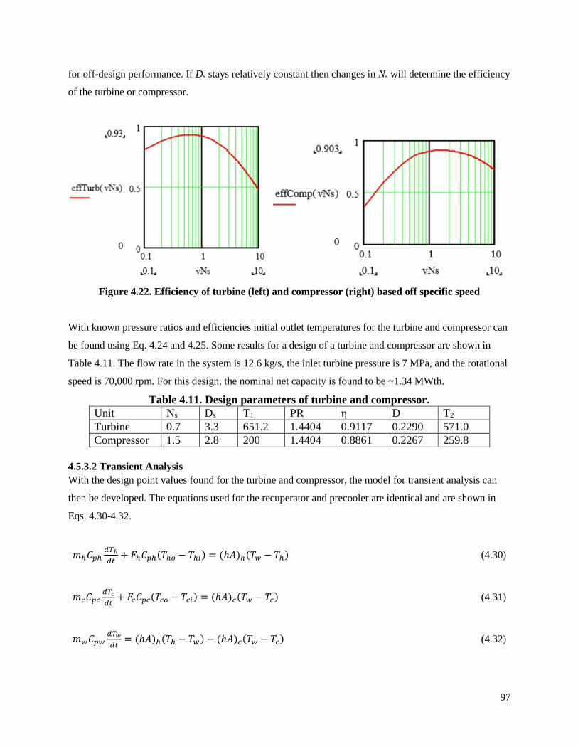
97
for off-design performance. If Ds stays relatively constant then changes in Ns will determine the efficiency
of the turbine or compressor.
Figure 4.22. Efficiency of turbine (left) and compressor (right) based off specific speed
With known pressure ratios and efficiencies initial outlet temperatures for the turbine and compressor can
be found using Eq. 4.24 and 4.25. Some results for a design of a turbine and compressor are shown in
Table 4.11. The flow rate in the system is 12.6 kg/s, the inlet turbine pressure is 7 MPa, and the rotational
speed is 70,000 rpm. For this design, the nominal net capacity is found to be ~1.34 MWth.
Table 4.11. Design parameters of turbine and compressor.
Unit Ns Ds T1 PR η D T2
Turbine 0.7 3.3 651.2 1.4404 0.9117 0.2290 571.0
Compressor 1.5 2.8 200 1.4404 0.8861 0.2267 259.8
4.5.3.2 Transient Analysis
With the design point values found for the turbine and compressor, the model for transient analysis can
then be developed. The equations used for the recuperator and precooler are identical and are shown in
Eqs. 4.30-4.32.
𝑚ℎ𝐶𝑝ℎ𝑑𝑇ℎ
𝑑𝑡+ 𝐹ℎ𝐶𝑝ℎ(𝑇ℎ𝑜 − 𝑇ℎ𝑖) = (ℎ𝐴)ℎ(𝑇𝑤 − 𝑇ℎ) (4.30)
𝑚𝑐𝐶𝑝𝑐𝑑𝑇𝑐
𝑑𝑡+ 𝐹𝑐𝐶𝑝𝑐(𝑇𝑐𝑜 − 𝑇𝑐𝑖) = (ℎ𝐴)𝑐(𝑇𝑤 − 𝑇𝑐) (4.31)
𝑚𝑤𝐶𝑝𝑤𝑑𝑇𝑤
𝑑𝑡= (ℎ𝐴)ℎ(𝑇ℎ − 𝑇𝑤) − (ℎ𝐴)𝑐(𝑇𝑤 − 𝑇𝑐) (4.32)
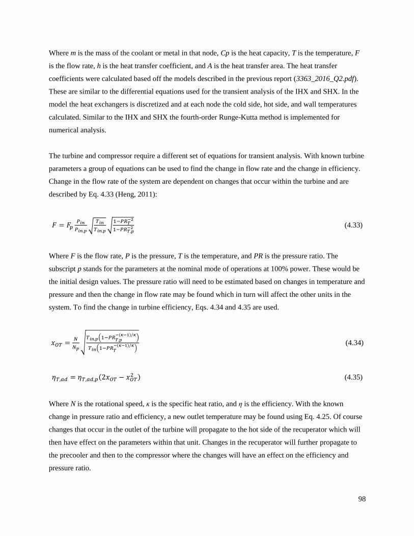
98
Where m is the mass of the coolant or metal in that node, Cp is the heat capacity, T is the temperature, F
is the flow rate, h is the heat transfer coefficient, and A is the heat transfer area. The heat transfer
coefficients were calculated based off the models described in the previous report (3363_2016_Q2.pdf).
These are similar to the differential equations used for the transient analysis of the IHX and SHX. In the
model the heat exchangers is discretized and at each node the cold side, hot side, and wall temperatures
calculated. Similar to the IHX and SHX the fourth-order Runge-Kutta method is implemented for
numerical analysis.
The turbine and compressor require a different set of equations for transient analysis. With known turbine
parameters a group of equations can be used to find the change in flow rate and the change in efficiency.
Change in the flow rate of the system are dependent on changes that occur within the turbine and are
described by Eq. 4.33 (Heng, 2011):
𝐹 = 𝐹𝑝𝑃𝑖𝑛
𝑃𝑖𝑛,𝑝√
𝑇𝑖𝑛
𝑇𝑖𝑛,𝑝√
1−𝑃𝑅𝑇−2
1−𝑃𝑅𝑇,𝑝−2 (4.33)
Where F is the flow rate, P is the pressure, T is the temperature, and PR is the pressure ratio. The
subscript p stands for the parameters at the nominal mode of operations at 100% power. These would be
the initial design values. The pressure ratio will need to be estimated based on changes in temperature and
pressure and then the change in flow rate may be found which in turn will affect the other units in the
system. To find the change in turbine efficiency, Eqs. 4.34 and 4.35 are used.
𝑥𝑂𝑇 =𝑁
𝑁𝑝√
𝑇𝑖𝑛,𝑝(1−𝑃𝑅𝑇,𝑝−(𝜅−1)/𝜅
)
𝑇𝑖𝑛(1−𝑃𝑅𝑇−(𝜅−1)/𝜅
) (4.34)
𝜂𝑇,𝑎𝑑 = 𝜂𝑇,𝑎𝑑,𝑝(2𝑥𝑂𝑇 − 𝑥𝑂𝑇2 ) (4.35)
Where N is the rotational speed, ĸ is the specific heat ratio, and η is the efficiency. With the known
change in pressure ratio and efficiency, a new outlet temperature may be found using Eq. 4.25. Of course
changes that occur in the outlet of the turbine will propagate to the hot side of the recuperator which will
then have effect on the parameters within that unit. Changes in the recuperator will further propagate to
the precooler and then to the compressor where the changes will have an effect on the efficiency and
pressure ratio.
99
Transient analysis for a compressor is slightly trickier as it requires a compressor map to predict changes
efficiency and pressure ratio. These are typically created from the experimental data for that particular
compressor. They vary from compressor to compressor so it can be difficult to create this without the
necessary information. These charts require corrected match flow rare (Fcor) and corrected rotational
speed (Ncor) and are defined in Eqs. 4.36 and 4.37 (Wenlong et al, 2012).
𝐹𝑐𝑜𝑟 =𝐹
𝐹𝑝
101325
𝑃𝐶,𝑖𝑛√
288
𝑇𝐶,𝑖𝑛 (4.36)
𝑁𝑐𝑜𝑟 =𝑁
𝑁𝑝√
288
𝑇𝐶,𝑖𝑛 (4.37)
Where the subscript cor stands for correct mass flow rate (F) or corrected rotational speed (N). A typical
compressor map is shown in Figure 4.23. The map shows the pressure ratio as a function of the
normalized flow rate, with the dashed lines representing the constant efficiency curves. The solid lines
represent constant speed with the speed increasing from left to right. This chart is used to find the new
pressure ratio and compressor efficiency, if parameters in the compressor change such as inlet
temperature, inlet pressure or flow rate.
Figure 4.23. Typical compressor performance curve
This typical performance curve can be used to create charts that can represent the system. Assuming the
compressor is designed at the most optimal point, we have values for the pressure ratio and corrected
mass flow rate at that point. The WebPlotDigitizer tool (http://arohatgi.info/WebPlotDigitizer/) can be

100
used to convert obtain numerical values of x-y coordinates of different curves from the performance chart,
such as the one shown in Figure 4.23. From these data, charts can be created and best fit lines made that
can be included in the model code. Figure 4.24 and 4.25 show the performance curves created from
Figure 4.23. In Figure 4.24 the corrected mass flow rate (x-axis) is used to find the pressure ratio (y-axis).
Each of the curves represents different rotational speed, with the green line (100%) representing the
design speed. Figure 4.25 uses the corrected mass flow rate (x-axis) to find the efficiency (y-axis) of the
compressor. Similarly, each of the lines represents different rotational speed, with the green line (100%)
representing the design speed. A large change in the corrected mass flow rate requires changing the
rotational speed to maintain high efficiency. For example, from Figure 4.25, the compressor efficiency at
the corrected mass flow rate of 0.025 and 100% speed (green line) is close to 90%. If the corrected mass
flow rate were to decrease to 0.0235, then the compressor efficiency at the design speed is only ~70%. In
this case, higher efficiency can be achieved by decreasing the speed to 90% of the design value, raising
the efficiency to ~85%. Figure 4.24 can then be used to obtain the pressure ratio, and the outlet pressure.
Thus, the changes in outlet conditions in response to changes in the inlet conditions could be found.
Figure 4.24. Performance curves to find compressor pressure ratio.
1
1.1
1.2
1.3
1.4
1.5
1.6
1.7
0.02 0.0225 0.025 0.0275
PR
c
Fcor
80%
90%
100%
110%
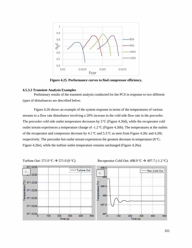
101
Figure 4.25. Performance curves to find compressor efficiency.
4.5.3.3 Transient Analysis Examples
Preliminary results of the transient analysis conducted for the PCS in response to two different
types of disturbances are described below.
Figure 4.26 shows an example of the system response in terms of the temperatures of various
streams to a flow rate disturbance involving a 20% increase in the cold side flow rate in the precooler.
The precooler cold side outlet temperature decreases by 3 oC (Figure 4.26d), while the recuperator cold
outlet stream experiences a temperature change of -1.2 oC (Figure 4.26b). The temperatures at the outlets
of the recuperator and compressor decrease by 4.1 oC and 5.3 oC as seen from Figure 4.26c and 4.26f,
respectively. The precooler hot outlet stream experiences the greatest decrease in temperature (8 oC,
Figure 4.26e), while the turbine outlet temperature remains unchanged (Figure 4.26a).
Turbine Out: 571.0 oC 571.0 (0 oC) Recuperator Cold Out: 498.9 oC 497.7 (-1.2 oC)
0.4
0.5
0.6
0.7
0.8
0.9
1
0.02 0.0225 0.025 0.0275
η_c
Fcor
80%
90%
100%
110%
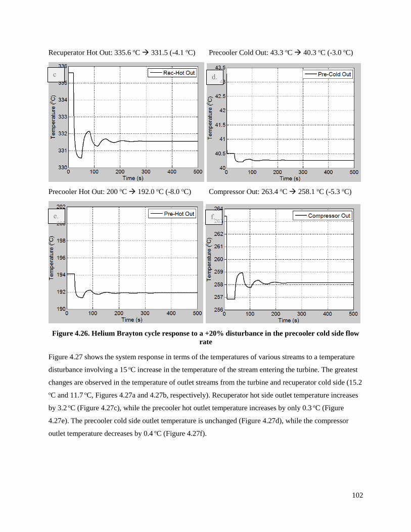
102
Recuperator Hot Out: 335.6 oC 331.5 (-4.1 oC) Precooler Cold Out: 43.3 oC 40.3 oC (-3.0 oC)
Precooler Hot Out: 200 oC 192.0 oC (-8.0 oC) Compressor Out: 263.4 oC 258.1 oC (-5.3 oC)
Figure 4.26. Helium Brayton cycle response to a +20% disturbance in the precooler cold side flow
rate
Figure 4.27 shows the system response in terms of the temperatures of various streams to a temperature
disturbance involving a 15 oC increase in the temperature of the stream entering the turbine. The greatest
changes are observed in the temperature of outlet streams from the turbine and recuperator cold side (15.2
oC and 11.7 oC, Figures 4.27a and 4.27b, respectively). Recuperator hot side outlet temperature increases
by 3.2 oC (Figure 4.27c), while the precooler hot outlet temperature increases by only 0.3 oC (Figure
4.27e). The precooler cold side outlet temperature is unchanged (Figure 4.27d), while the compressor
outlet temperature decreases by 0.4 oC (Figure 4.27f).
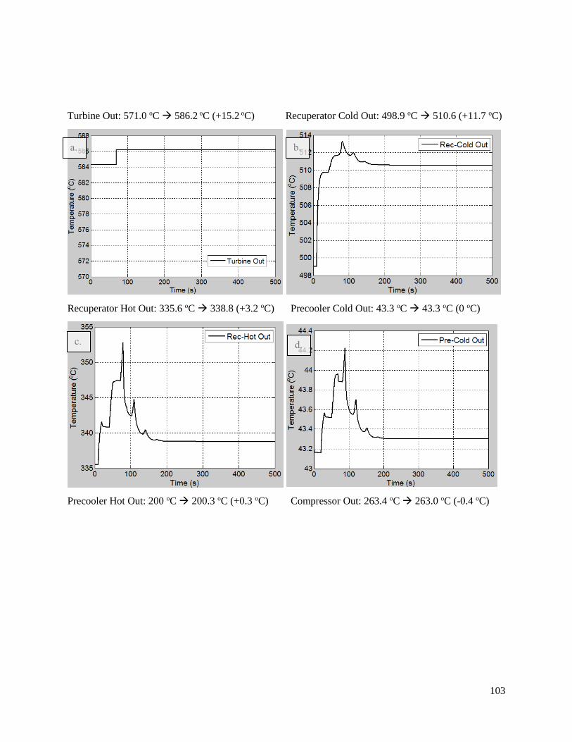
103
Turbine Out: 571.0 oC 586.2 oC (+15.2 oC) Recuperator Cold Out: 498.9 oC 510.6 (+11.7 oC)
Recuperator Hot Out: 335.6 oC 338.8 (+3.2 oC) Precooler Cold Out: 43.3 oC 43.3 oC (0 oC)
Precooler Hot Out: 200 oC 200.3 oC (+0.3 oC) Compressor Out: 263.4 oC 263.0 oC (-0.4 oC)
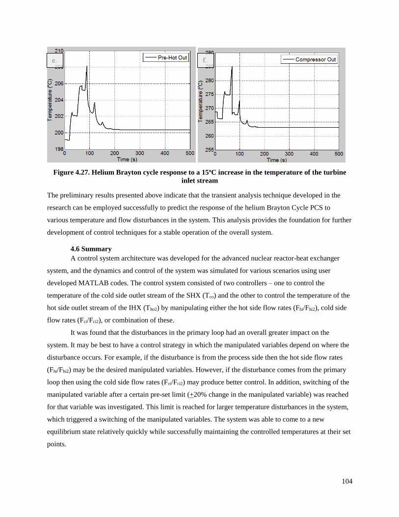
104
Figure 4.27. Helium Brayton cycle response to a 15oC increase in the temperature of the turbine
inlet stream
The preliminary results presented above indicate that the transient analysis technique developed in the
research can be employed successfully to predict the response of the helium Brayton Cycle PCS to
various temperature and flow disturbances in the system. This analysis provides the foundation for further
development of control techniques for a stable operation of the overall system.
4.6 Summary
A control system architecture was developed for the advanced nuclear reactor-heat exchanger
system, and the dynamics and control of the system was simulated for various scenarios using user
developed MATLAB codes. The control system consisted of two controllers – one to control the
temperature of the cold side outlet stream of the SHX (Tco) and the other to control the temperature of the
hot side outlet stream of the IHX (Tho2) by manipulating either the hot side flow rates (Fhi/Fhi2), cold side
flow rates (Fci/Fci2), or combination of these.
It was found that the disturbances in the primary loop had an overall greater impact on the
system. It may be best to have a control strategy in which the manipulated variables depend on where the
disturbance occurs. For example, if the disturbance is from the process side then the hot side flow rates
(Fhi/Fhi2) may be the desired manipulated variables. However, if the disturbance comes from the primary
loop then using the cold side flow rates (Fci/Fci2) may produce better control. In addition, switching of the
manipulated variable after a certain pre-set limit (+20% change in the manipulated variable) was reached
for that variable was investigated. This limit is reached for larger temperature disturbances in the system,
which triggered a switching of the manipulated variables. The system was able to come to a new
equilibrium state relatively quickly while successfully maintaining the controlled temperatures at their set
points.

105
The behavior of the system under a comprehensive control scheme where the nuclear reactor
operation is also controlled was also simulated. The reactor model included the point kinetic equations
with 3 groups of delayed neutrons, which achieved the best balance between the computational load and
accuracy. Two types of control strategies were implemented into the model. The first was identical to the
first MATLAB model and involved 2 controllers in which the cold side outlet temperature of the SHX
(Tco) and hot side outlet temperature of the IHX (Tho2) are controlled by manipulation of the hot side flow
rate of the SHX (Fhi) and hot side flow rate of the IHX (Fhi2). Temperature disturbances of ±10 oC
required flow rate changes of ±2-8% of their initial value to properly control the system. Flow rate
disturbances of ±10% Fc required a larger change in flow rate of ±11-18% of their initial values for
control. The second control strategy involved the control of the cold outlet temperature of the SHX (Tco)
using 3 different control options. The first involved manipulating the flow rate, the second controlling the
reactor power and the third a combination of the first two options. The final control option combines the
advantages from the other two control options – rapidity of the response from option one, and minimal
flow rate change from option two – and is potentially a superior option compared to the first two.
A comprehensive model was developed to obtain the dynamics of the helium Brayton Cycle PCS in
response to any system disturbances. The recuperator and precooler were modeled similarly to the any
other heat exchanger, while a novel technique was used for the turbine and the compressor. Temperature
transients of various streams in response to different disturbance stimuli were obtained indicating the
utility of this approach.
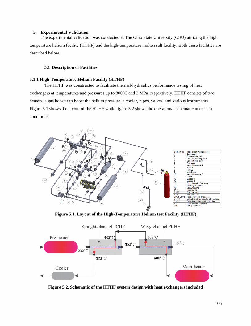
106
5. Experimental Validation
The experimental validation was conducted at The Ohio State University (OSU) utilizing the high
temperature helium facility (HTHF) and the high-temperature molten salt facility. Both these facilities are
described below.
5.1 Description of Facilities
5.1.1 High-Temperature Helium Facility (HTHF)
The HTHF was constructed to facilitate thermal-hydraulics performance testing of heat
exchangers at temperatures and pressures up to 800°C and 3 MPa, respectively. HTHF consists of two
heaters, a gas booster to boost the helium pressure, a cooler, pipes, valves, and various instruments.
Figure 5.1 shows the layout of the HTHF while figure 5.2 shows the operational schematic under test
conditions.
Figure 5.1. Layout of the High-Temperature Helium test Facility (HTHF)
Figure 5.2. Schematic of the HTHF system design with heat exchangers included

107
The mass flow rate in the loop used for the steady-state operation is 26.5 kg/h. The powers of the pre-
heater and main heater are 6.5 and 4.3 kW, respectively; and the heat rejection from the cooler to the
chilled water is at most 10.8 kW. The printed circuit heat exchanger (PCHE) in figure 2 refers to an
existing straight-channel PCHE, while the wavy-channel PCHE refers to the heat exchangers fabricated
for this project. Temperatures shown in the figure are representative of the operating conditions during the
testing of the heat exchangers.
5.1.2 High-Temperature Molten Salt Facility
The layout of the base configuration of the scaled-down high-temperature liquid fluoride salt facility at
OSU is shown in Figure 5.3. This multipurpose facility is used for various projects. The base
configuration indicates its use for reactor auxiliary cooling via DHX (Direct Reactor Auxiliary Cooling
System Heat Exchanger) and NDHX (Natural Draft Heat Exchanger). The facility was modified for IHX
testing as described later in the report.
Figure 5.3. 3D Layout of the high temperature molten salt test facility
This facility is designed to for handling fluoride salts. Two different salts can be used in the
system. The facility can also handle most other fluids unless there is a materials compatibility
issue between the fluids and the material of construction. The other key component of the loop is
the heater core, which is rated nominally at 70 kW.
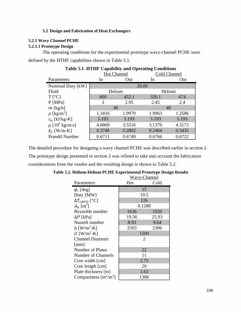
108
5.2 Design and Fabrication of Heat Exchangers
5.2.1 Wavy Channel PCHE
5.2.1.1 Prototype Design
The operating conditions for the experimental prototype wavy-channel PCHE were
defined by the HTHF capabilities shown in Table 5.1.
Table 5.1. HTHF Capability and Operating Conditions
Parameters
Hot Channel
In Out
Cold Channel
In Out
Nominal Duty [kW] 20.00
Fluid Helium Helium
T [°C] 800 452.1 326.1 674
P [MPa] 3 2.95 2.45 2.4
�̇� [kg/h] 40 40
𝜌 [kg/m3] 1.3416 1.9970 1.9963 1.2586
𝑐𝑝 [kJ/kg-K] 5.193 5.193 5.193 5.193
𝜇 [105 kg/m-s] 4.6869 3.5516 3.1370 4.3172
𝑘𝑓 [W/m-K] 0.3746 0.2802 0.2464 0.3435
Prandtl Number 0.6711 0.6749 0.6766 0.6722
The detailed procedure for designing a wavy channel PCHE was described earlier in section 2.
The prototype design presented in section 2 was refined to take into account the fabrication
considerations from the vendor and the resulting design is shown in Table 5.2.
Table 5.2. Helium-Helium PCHE Experimental Prototype Design Results
Parameters
Wavy-Channel
Hot Cold
𝜙, [deg] 15
Duty [MW] 19.5
∆𝑇𝐿𝑀𝑇𝐷 [°C] 126
𝐴ℎ [m2] 0.1288
Reynolds number 1636 1920
∆𝑃 [kPa] 19.56 25.93
Nusselt number 8.93 9.64
ℎ [W/m2-K] 2503 2306
𝑈 [W/m2-K] 1200
Channel Diameter
[mm]
2
Number of Plates 22
Number of Channels 11
Core width [cm] 2.75
Core length [cm] 20
Plate thickness [m] 1.63
Compactness [m2/m3] 1306
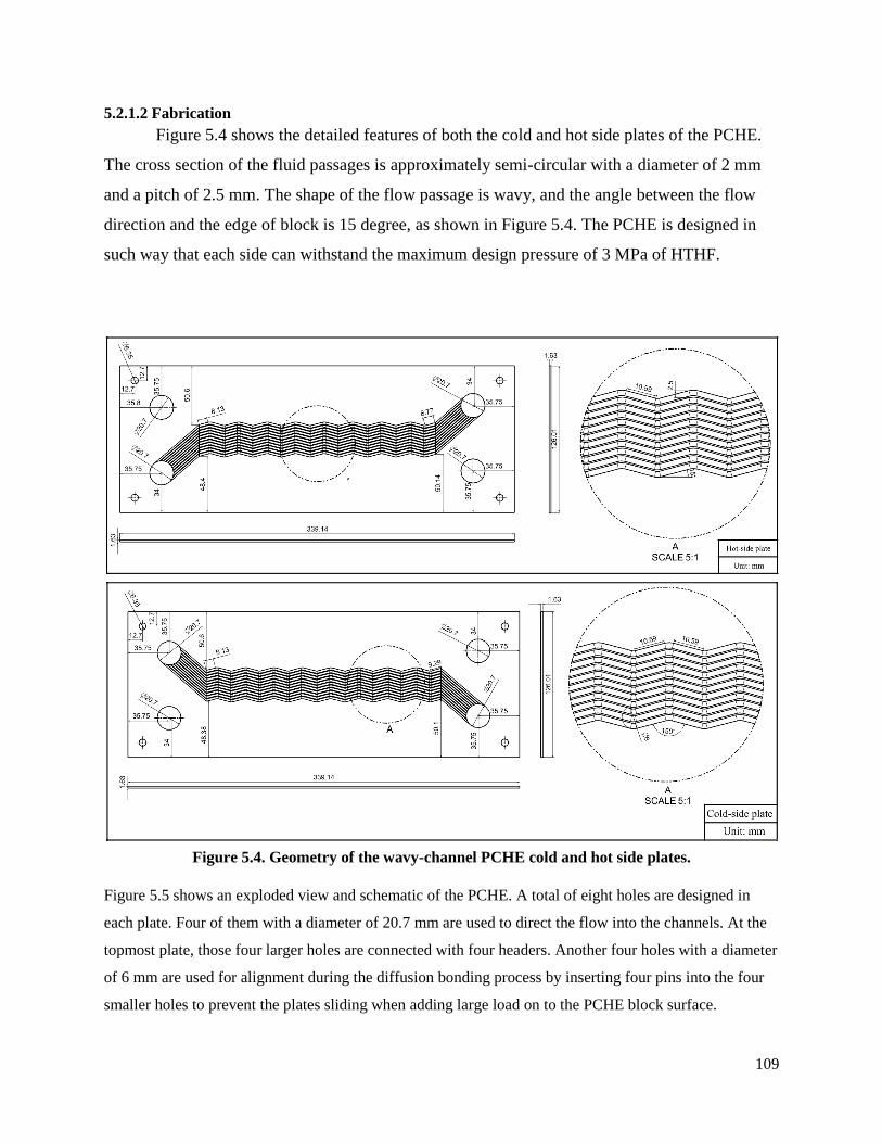
109
5.2.1.2 Fabrication
Figure 5.4 shows the detailed features of both the cold and hot side plates of the PCHE.
The cross section of the fluid passages is approximately semi-circular with a diameter of 2 mm
and a pitch of 2.5 mm. The shape of the flow passage is wavy, and the angle between the flow
direction and the edge of block is 15 degree, as shown in Figure 5.4. The PCHE is designed in
such way that each side can withstand the maximum design pressure of 3 MPa of HTHF.
Figure 5.4. Geometry of the wavy-channel PCHE cold and hot side plates.
Figure 5.5 shows an exploded view and schematic of the PCHE. A total of eight holes are designed in
each plate. Four of them with a diameter of 20.7 mm are used to direct the flow into the channels. At the
topmost plate, those four larger holes are connected with four headers. Another four holes with a diameter
of 6 mm are used for alignment during the diffusion bonding process by inserting four pins into the four
smaller holes to prevent the plates sliding when adding large load on to the PCHE block surface.

110
The dimensions of the PCHE block shown in Figure 5.4 were 12 inches in length by 4.4 inches in width,
and 2.35 inches thick. The thicknesses of the topmost plate and bottommost plate was both 0.5 inch. The
topmost plate provides a strong base for joining the four headers. The headers are made from 1 inch NPS
pipes since the piping size in the test facility is 1 inch NPS (corresponding to a pipe schedule of 160).
The flow passages in each plate of the PCHE were made by applying a photochemical etching technique,
which uses strong chemical etchants to remove unwanted work piece material on the surface of the plates
by controlled dissolution. All eight holes in the plates and the spaces between the channels and 20.7 mm-
diameter holes were also made during this chemical etching process.
Figure 5.5. The exploded view and schematic of the PCHE
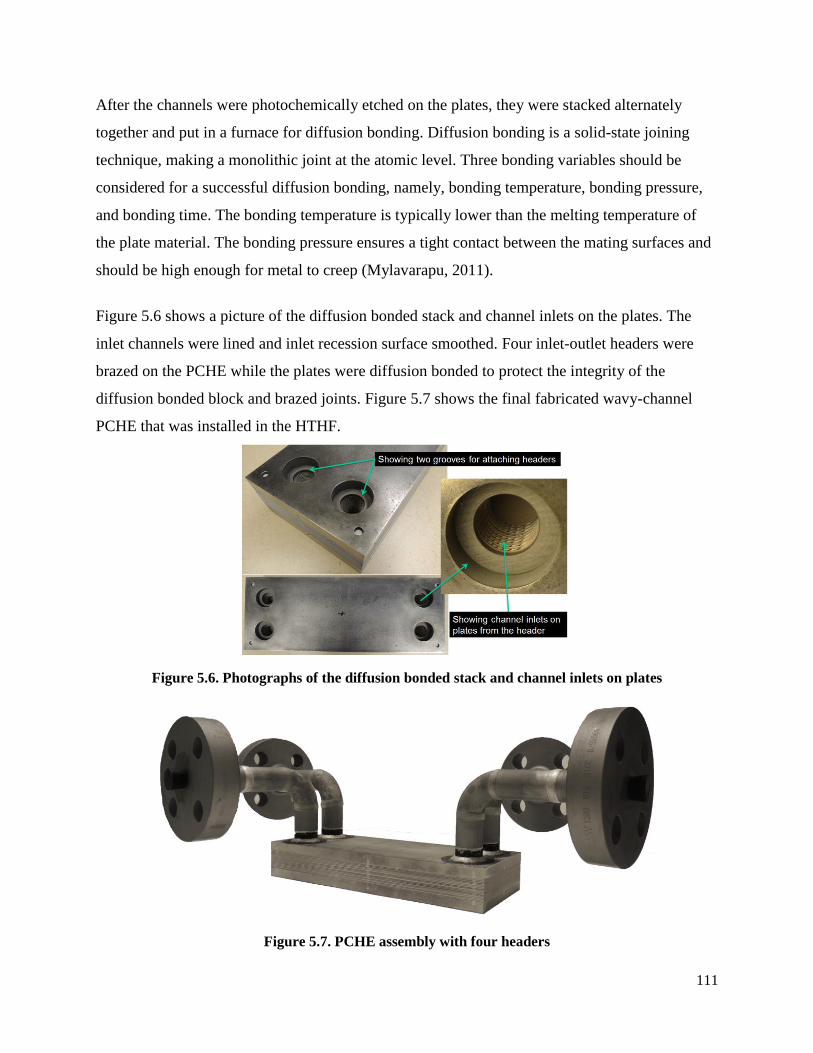
111
After the channels were photochemically etched on the plates, they were stacked alternately
together and put in a furnace for diffusion bonding. Diffusion bonding is a solid-state joining
technique, making a monolithic joint at the atomic level. Three bonding variables should be
considered for a successful diffusion bonding, namely, bonding temperature, bonding pressure,
and bonding time. The bonding temperature is typically lower than the melting temperature of
the plate material. The bonding pressure ensures a tight contact between the mating surfaces and
should be high enough for metal to creep (Mylavarapu, 2011).
Figure 5.6 shows a picture of the diffusion bonded stack and channel inlets on the plates. The
inlet channels were lined and inlet recession surface smoothed. Four inlet-outlet headers were
brazed on the PCHE while the plates were diffusion bonded to protect the integrity of the
diffusion bonded block and brazed joints. Figure 5.7 shows the final fabricated wavy-channel
PCHE that was installed in the HTHF.
Figure 5.6. Photographs of the diffusion bonded stack and channel inlets on plates
Figure 5.7. PCHE assembly with four headers
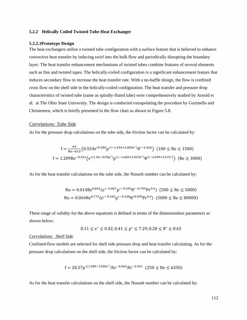
112
5.2.2 Helically Coiled Twisted Tube Heat Exchanger
5.2.2.1Prototype Design
The heat exchangers utilize a twisted tube configuration with a surface feature that is believed to enhance
convective heat transfer by inducing swirl into the bulk flow and periodically disrupting the boundary
layer. The heat transfer enhancement mechanisms of twisted tubes combine features of several elements
such as fins and twisted tapes. The helically-coiled configuration is a significant enhancement feature that
induces secondary flow to increase the heat transfer rate. With a no-baffle design, the flow is confined
cross flow on the shell side in the helically-coiled configuration. The heat transfer and pressure drop
characteristics of twisted tube (same as spirally-fluted tube) were comprehensively studied by Arnold et
al. at The Ohio State University. The design is conducted extrapolating the procedure by Garimella and
Christensen, which is briefly presented in the flow chart as shown in Figure 5.8.
Correlations: Tube Side
As for the pressure drop calculations on the tube side, the friction factor can be calculated by:
f =64
Re−45.0(0.554e∗0.384p∗(−1.454+2.083e∗)θ∗−2.426) (100 ≤ Re ≤ 1500)
f = 1.209Re−0.261(e∗(1.26−0.05p∗)p∗(−1.660+2.033e∗)θ∗(−2.699+3.67e∗)) (Re ≥ 3000)
As for the heat transfer calculations on the tube side, the Nusselt number can be calculated by:
Nu = 0.014Re0.842(e∗−0.067p∗−0.293θ∗−0.705Pr0.4) (500 ≤ Re ≤ 5000)
Nu = 0.064Re0.773(e∗−0.242p∗−0.108θ∗0.599Pr0.4) (5000 ≤ Re ≤ 80000)
These range of validity for the above equations is defined in terms of the dimensionless parameters as
shown below:
0.11 ≤ e∗ ≤ 0.42; 0.41 ≤ p∗ ≤ 7.29; 0.28 ≤ θ∗ ≤ 0.65
Correlations: Shell Side
Confined-flow models are selected for shell side pressure drop and heat transfer calculating. As for the
pressure drop calculations on the shell side, the friction factor can be calculated by:
f = 20.57𝑝∗(1.089−1500𝑒∗)𝑅𝑒−0.463𝑁𝑡−0.351 (250 ≤ Re ≤ 6350)
As for the heat transfer calculations on the shell side, the Nusselt number can be calculated by:
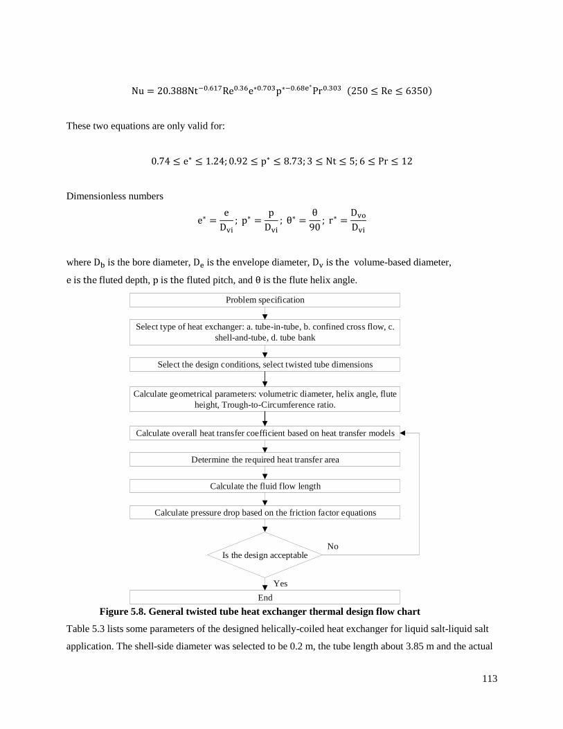
113
Nu = 20.388Nt−0.617Re0.36e∗0.703p∗−0.68e∗Pr0.303 (250 ≤ Re ≤ 6350)
These two equations are only valid for:
0.74 ≤ e∗ ≤ 1.24; 0.92 ≤ p∗ ≤ 8.73; 3 ≤ Nt ≤ 5; 6 ≤ Pr ≤ 12
Dimensionless numbers
e∗ =e
Dvi; p∗ =
p
Dvi; θ∗ =
θ
90; r∗ =
Dvo
Dvi
where Db is the bore diameter, De is the envelope diameter, Dv is the volume-based diameter,
e is the fluted depth, p is the fluted pitch, and θ is the flute helix angle.
Problem specification
Select the design conditions, select twisted tube dimensions
Select type of heat exchanger: a. tube-in-tube, b. confined cross flow, c.
shell-and-tube, d. tube bank
Calculate overall heat transfer coefficient based on heat transfer models
Determine the required heat transfer area
Calculate the fluid flow length
Calculate pressure drop based on the friction factor equations
Is the design acceptable
End
No
Yes
Calculate geometrical parameters: volumetric diameter, helix angle, flute
height, Trough-to-Circumference ratio.
Figure 5.8. General twisted tube heat exchanger thermal design flow chart
Table 5.3 lists some parameters of the designed helically-coiled heat exchanger for liquid salt-liquid salt
application. The shell-side diameter was selected to be 0.2 m, the tube length about 3.85 m and the actual
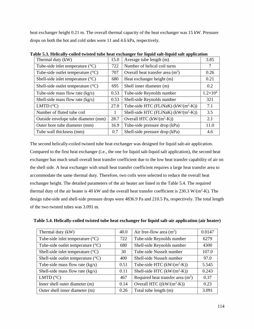
114
heat exchanger height 0.21 m. The overall thermal capacity of the heat exchanger was 15 kW. Pressure
drops on both the hot and cold sides were 11 and 4.6 kPa, respectively.
Table 5.3. Helically-coiled twisted tube heat exchanger for liquid salt-liquid salt application
Thermal duty (kW) 15.0 Average tube length (m) 3.85
Tube-side inlet temperature (°C) 722 Number of helical coil turns 7
Tube-side outlet temperature (°C) 707 Overall heat transfer area (m2) 0.26
Shell-side inlet temperature (°C) 680 Heat exchanger height (m) 0.21
Shell-side outlet temperature (°C) 695 Shell inner diameter (m) 0.2
Tube-side mass flow rate (kg/s) 0.53 Tube-side Reynolds number 1.2×10⁴
Shell-side mass flow rate (kg/s) 0.53 Shell-side Reynolds number 321
LMTD (°C) 27.0 Tube-side HTC (FLiNaK) (kW/(m2-K)) 7.1
Number of fluted tube coil 1 Shell-side HTC (FLiNaK) (kW/(m2-K)) 3.5
Outside envelope tube diameter (mm) 28.7 Overall HTC (kW/(m2-K)) 2.1
Outer bore tube diameter (mm) 16.9 Tube-side pressure drop (kPa) 11.0
Tube wall thickness (mm) 0.7 Shell-side pressure drop (kPa) 4.6
The second helically-coiled twisted tube heat exchanger was designed for liquid salt-air application.
Compared to the first heat exchanger (i.e., the one for liquid salt-liquid salt application), the second heat
exchanger has much small overall heat transfer coefficient due to the low heat transfer capability of air on
the shell side. A heat exchanger with small heat transfer coefficient requires a large heat transfer area to
accommodate the same thermal duty. Therefore, two coils were selected to reduce the overall heat
exchanger height. The detailed parameters of the air heater are listed in the Table 5.4. The required
thermal duty of the air heater is 40 kW and the overall heat transfer coefficient is 230.3 W/(m2-K). The
design tube-side and shell-side pressure drops were 4836.9 Pa and 210.5 Pa, respectively. The total length
of the two twisted tubes was 3.091 m.
Table 5.4. Helically-coiled twisted tube heat exchanger for liquid salt-air application (air heater)
Thermal duty (kW) 40.0 Air free-flow area (m2) 0.0147
Tube-side inlet temperature (°C) 722 Tube-side Reynolds number 6279
Tube-side outlet temperature (°C) 680 Shell-side Reynolds number 4300
Shell-side inlet temperature (°C) 30 Tube-side Nusselt number 107.0
Shell-side outlet temperature (°C) 400 Shell-side Nusselt number 97.0
Tube-side mass flow rate (kg/s) 0.51 Tube-side HTC (kW/(m2-K)) 5.545
Shell-side mass flow rate (kg/s) 0.11 Shell-side HTC (kW/(m2-K)) 0.243
LMTD (°C) 467 Required heat transfer area (m2) 0.37
Inner shell outer diameter (m) 0.14 Overall HTC ((kW/(m2-K)) 0.23
Outer shell inner diameter (m) 0.26 Total tube length (m) 3.091
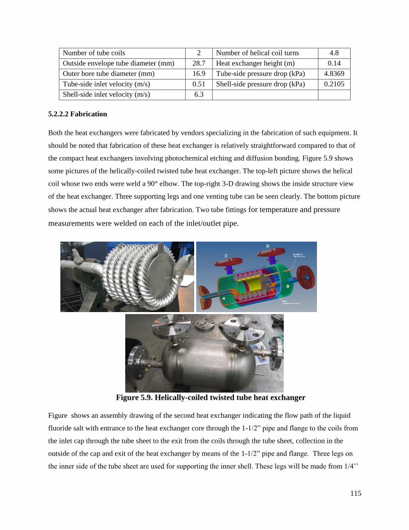
115
Number of tube coils 2 Number of helical coil turns 4.8
Outside envelope tube diameter (mm) 28.7 Heat exchanger height (m) 0.14
Outer bore tube diameter (mm) 16.9 Tube-side pressure drop (kPa) 4.8369
Tube-side inlet velocity (m/s) 0.51 Shell-side pressure drop (kPa) 0.2105
Shell-side inlet velocity (m/s) 6.3
5.2.2.2 Fabrication
Both the heat exchangers were fabricated by vendors specializing in the fabrication of such equipment. It
should be noted that fabrication of these heat exchanger is relatively straightforward compared to that of
the compact heat exchangers involving photochemical etching and diffusion bonding. Figure 5.9 shows
some pictures of the helically-coiled twisted tube heat exchanger. The top-left picture shows the helical
coil whose two ends were weld a 90° elbow. The top-right 3-D drawing shows the inside structure view
of the heat exchanger. Three supporting legs and one venting tube can be seen clearly. The bottom picture
shows the actual heat exchanger after fabrication. Two tube fittings for temperature and pressure
measurements were welded on each of the inlet/outlet pipe.
Figure 5.9. Helically-coiled twisted tube heat exchanger
Figure shows an assembly drawing of the second heat exchanger indicating the flow path of the liquid
fluoride salt with entrance to the heat exchanger core through the 1-1/2” pipe and flange to the coils from
the inlet cap through the tube sheet to the exit from the coils through the tube sheet, collection in the
outside of the cap and exit of the heat exchanger by means of the 1-1/2” pipe and flange. Three legs on
the inner side of the tube sheet are used for supporting the inner shell. These legs will be made from 1/4’’
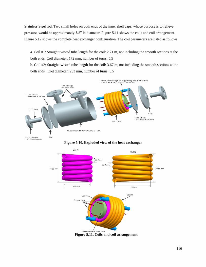
116
Stainless Steel rod. Two small holes on both ends of the inner shell caps, whose purpose is to relieve
pressure, would be approximately 3/8” in diameter. Figure 5.11 shows the coils and coil arrangement.
Figure 5.12 shows the complete heat exchanger configuration. The coil parameters are listed as follows:
a. Coil #1: Straight twisted tube length for the coil: 2.71 m, not including the smooth sections at the
both ends. Coil diameter: 172 mm, number of turns: 5.5
b. Coil #2: Straight twisted tube length for the coil: 3.67 m, not including the smooth sections at the
both ends. Coil diameter: 233 mm, number of turns: 5.5
Figure 5.10. Exploded view of the heat exchanger
Figure 5.11. Coils and coil arrangement
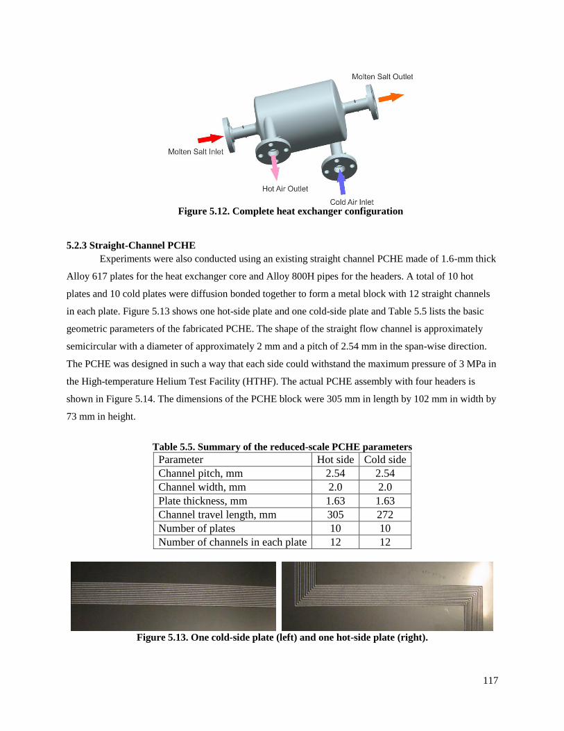
117
Figure 5.12. Complete heat exchanger configuration
5.2.3 Straight-Channel PCHE
Experiments were also conducted using an existing straight channel PCHE made of 1.6-mm thick
Alloy 617 plates for the heat exchanger core and Alloy 800H pipes for the headers. A total of 10 hot
plates and 10 cold plates were diffusion bonded together to form a metal block with 12 straight channels
in each plate. Figure 5.13 shows one hot-side plate and one cold-side plate and Table 5.5 lists the basic
geometric parameters of the fabricated PCHE. The shape of the straight flow channel is approximately
semicircular with a diameter of approximately 2 mm and a pitch of 2.54 mm in the span-wise direction.
The PCHE was designed in such a way that each side could withstand the maximum pressure of 3 MPa in
the High-temperature Helium Test Facility (HTHF). The actual PCHE assembly with four headers is
shown in Figure 5.14. The dimensions of the PCHE block were 305 mm in length by 102 mm in width by
73 mm in height.
Table 5.5. Summary of the reduced-scale PCHE parameters
Parameter Hot side Cold side
Channel pitch, mm 2.54 2.54
Channel width, mm 2.0 2.0
Plate thickness, mm 1.63 1.63
Channel travel length, mm 305 272
Number of plates 10 10
Number of channels in each plate 12 12
Figure 5.13. One cold-side plate (left) and one hot-side plate (right).
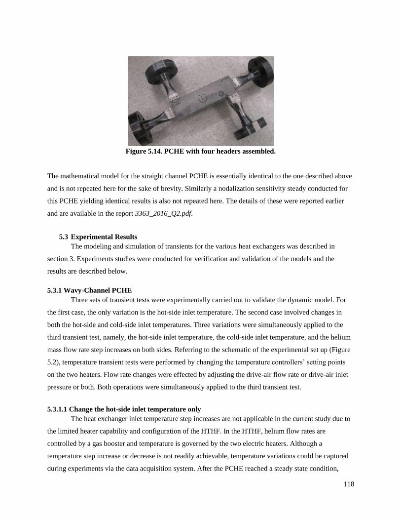
118
Figure 5.14. PCHE with four headers assembled.
The mathematical model for the straight channel PCHE is essentially identical to the one described above
and is not repeated here for the sake of brevity. Similarly a nodalization sensitivity steady conducted for
this PCHE yielding identical results is also not repeated here. The details of these were reported earlier
and are available in the report 3363_2016_Q2.pdf.
5.3 Experimental Results
The modeling and simulation of transients for the various heat exchangers was described in
section 3. Experiments studies were conducted for verification and validation of the models and the
results are described below.
5.3.1 Wavy-Channel PCHE
Three sets of transient tests were experimentally carried out to validate the dynamic model. For
the first case, the only variation is the hot-side inlet temperature. The second case involved changes in
both the hot-side and cold-side inlet temperatures. Three variations were simultaneously applied to the
third transient test, namely, the hot-side inlet temperature, the cold-side inlet temperature, and the helium
mass flow rate step increases on both sides. Referring to the schematic of the experimental set up (Figure
5.2), temperature transient tests were performed by changing the temperature controllers’ setting points
on the two heaters. Flow rate changes were effected by adjusting the drive-air flow rate or drive-air inlet
pressure or both. Both operations were simultaneously applied to the third transient test.
5.3.1.1 Change the hot-side inlet temperature only
The heat exchanger inlet temperature step increases are not applicable in the current study due to
the limited heater capability and configuration of the HTHF. In the HTHF, helium flow rates are
controlled by a gas booster and temperature is governed by the two electric heaters. Although a
temperature step increase or decrease is not readily achievable, temperature variations could be captured
during experiments via the data acquisition system. After the PCHE reached a steady state condition,
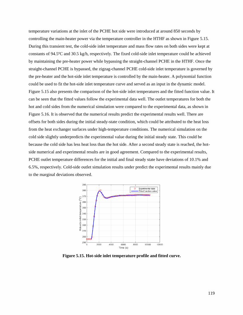
119
temperature variations at the inlet of the PCHE hot side were introduced at around 850 seconds by
controlling the main-heater power via the temperature controller in the HTHF as shown in Figure 5.15.
During this transient test, the cold-side inlet temperature and mass flow rates on both sides were kept at
constants of 94.5ºC and 30.5 kg/h, respectively. The fixed cold-side inlet temperature could be achieved
by maintaining the pre-heater power while bypassing the straight-channel PCHE in the HTHF. Once the
straight-channel PCHE is bypassed, the zigzag-channel PCHE cold-side inlet temperature is governed by
the pre-heater and the hot-side inlet temperature is controlled by the main-heater. A polynomial function
could be used to fit the hot-side inlet temperature curve and served as an input in the dynamic model.
Figure 5.15 also presents the comparison of the hot-side inlet temperatures and the fitted function value. It
can be seen that the fitted values follow the experimental data well. The outlet temperatures for both the
hot and cold sides from the numerical simulation were compared to the experimental data, as shown in
Figure 5.16. It is observed that the numerical results predict the experimental results well. There are
offsets for both sides during the initial steady-state condition, which could be attributed to the heat loss
from the heat exchanger surfaces under high-temperature conditions. The numerical simulation on the
cold side slightly underpredicts the experimental value during the initial steady state. This could be
because the cold side has less heat loss than the hot side. After a second steady state is reached, the hot-
side numerical and experimental results are in good agreement. Compared to the experimental results,
PCHE outlet temperature differences for the initial and final steady state have deviations of 10.1% and
6.5%, respectively. Cold-side outlet simulation results under predict the experimental results mainly due
to the marginal deviations observed.
Figure 5.15. Hot-side inlet temperature profile and fitted curve.
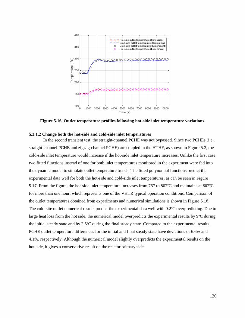
120
Figure 5.16. Outlet temperature profiles following hot-side inlet temperature variations.
5.3.1.2 Change both the hot-side and cold-side inlet temperatures
In the second transient test, the straight-channel PCHE was not bypassed. Since two PCHEs (i.e.,
straight-channel PCHE and zigzag-channel PCHE) are coupled in the HTHF, as shown in Figure 5.2, the
cold-side inlet temperature would increase if the hot-side inlet temperature increases. Unlike the first case,
two fitted functions instead of one for both inlet temperatures monitored in the experiment were fed into
the dynamic model to simulate outlet temperature trends. The fitted polynomial functions predict the
experimental data well for both the hot-side and cold-side inlet temperatures, as can be seen in Figure
5.17. From the figure, the hot-side inlet temperature increases from 767 to 802ºC and maintains at 802ºC
for more than one hour, which represents one of the VHTR typical operation conditions. Comparison of
the outlet temperatures obtained from experiments and numerical simulations is shown in Figure 5.18.
The cold-site outlet numerical results predict the experimental data well with 0.2ºC overpredicting. Due to
large heat loss from the hot side, the numerical model overpredicts the experimental results by 9ºC during
the initial steady state and by 2.5ºC during the final steady state. Compared to the experimental results,
PCHE outlet temperature differences for the initial and final steady state have deviations of 6.6% and
4.1%, respectively. Although the numerical model slightly overpredicts the experimental results on the
hot side, it gives a conservative result on the reactor primary side.
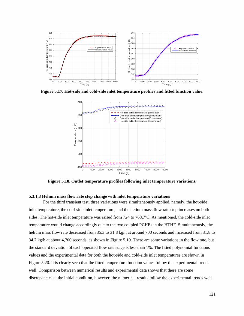
121
Figure 5.17. Hot-side and cold-side inlet temperature profiles and fitted function value.
Figure 5.18. Outlet temperature profiles following inlet temperature variations.
5.3.1.3 Helium mass flow rate step change with inlet temperature variations
For the third transient test, three variations were simultaneously applied, namely, the hot-side
inlet temperature, the cold-side inlet temperature, and the helium mass flow rate step increases on both
sides. The hot-side inlet temperature was raised from 724 to 768.7ºC. As mentioned, the cold-side inlet
temperature would change accordingly due to the two coupled PCHEs in the HTHF. Simultaneously, the
helium mass flow rate decreased from 35.3 to 31.8 kg/h at around 700 seconds and increased from 31.8 to
34.7 kg/h at about 4,700 seconds, as shown in Figure 5.19. There are some variations in the flow rate, but
the standard deviation of each operated flow rate stage is less than 1%. The fitted polynomial functions
values and the experimental data for both the hot-side and cold-side inlet temperatures are shown in
Figure 5.20. It is clearly seen that the fitted temperature function values follow the experimental trends
well. Comparison between numerical results and experimental data shows that there are some
discrepancies at the initial condition, however, the numerical results follow the experimental trends well

122
and are in a good agreement with the experimental data in the final steady state as can be seen in Figure
5.21. Compared to the experimental results, PCHE outlet temperature differences for the initial and final
steady state have deviations of 6.5% and 2.6%, respectively.
Figure 5.19. Helium mass flow rate step changes.
Figure 5.20. Hot-side and cold-side inlet temperature profiles and fitted function value.
Figure 5.21. Outlet temperature profiles following inlet temperature variations.
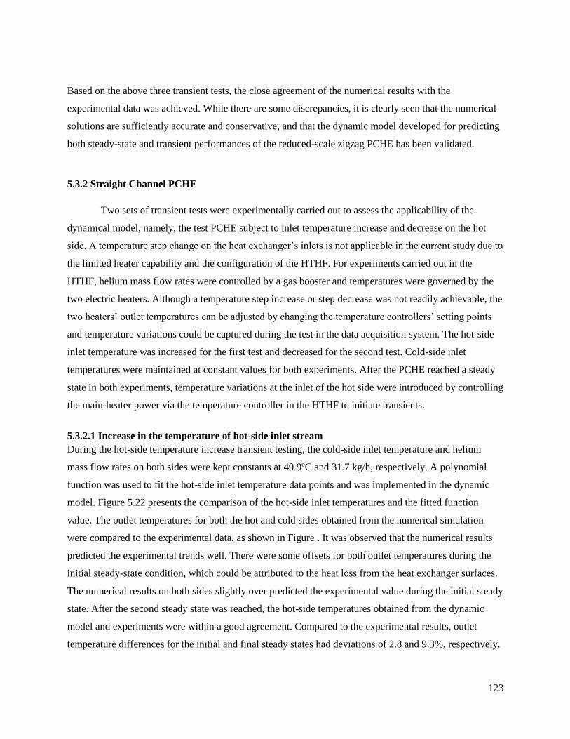
123
Based on the above three transient tests, the close agreement of the numerical results with the
experimental data was achieved. While there are some discrepancies, it is clearly seen that the numerical
solutions are sufficiently accurate and conservative, and that the dynamic model developed for predicting
both steady-state and transient performances of the reduced-scale zigzag PCHE has been validated.
5.3.2 Straight Channel PCHE
Two sets of transient tests were experimentally carried out to assess the applicability of the
dynamical model, namely, the test PCHE subject to inlet temperature increase and decrease on the hot
side. A temperature step change on the heat exchanger’s inlets is not applicable in the current study due to
the limited heater capability and the configuration of the HTHF. For experiments carried out in the
HTHF, helium mass flow rates were controlled by a gas booster and temperatures were governed by the
two electric heaters. Although a temperature step increase or step decrease was not readily achievable, the
two heaters’ outlet temperatures can be adjusted by changing the temperature controllers’ setting points
and temperature variations could be captured during the test in the data acquisition system. The hot-side
inlet temperature was increased for the first test and decreased for the second test. Cold-side inlet
temperatures were maintained at constant values for both experiments. After the PCHE reached a steady
state in both experiments, temperature variations at the inlet of the hot side were introduced by controlling
the main-heater power via the temperature controller in the HTHF to initiate transients.
5.3.2.1 Increase in the temperature of hot-side inlet stream
During the hot-side temperature increase transient testing, the cold-side inlet temperature and helium
mass flow rates on both sides were kept constants at 49.9ºC and 31.7 kg/h, respectively. A polynomial
function was used to fit the hot-side inlet temperature data points and was implemented in the dynamic
model. Figure 5.22 presents the comparison of the hot-side inlet temperatures and the fitted function
value. The outlet temperatures for both the hot and cold sides obtained from the numerical simulation
were compared to the experimental data, as shown in Figure . It was observed that the numerical results
predicted the experimental trends well. There were some offsets for both outlet temperatures during the
initial steady-state condition, which could be attributed to the heat loss from the heat exchanger surfaces.
The numerical results on both sides slightly over predicted the experimental value during the initial steady
state. After the second steady state was reached, the hot-side temperatures obtained from the dynamic
model and experiments were within a good agreement. Compared to the experimental results, outlet
temperature differences for the initial and final steady states had deviations of 2.8 and 9.3%, respectively.
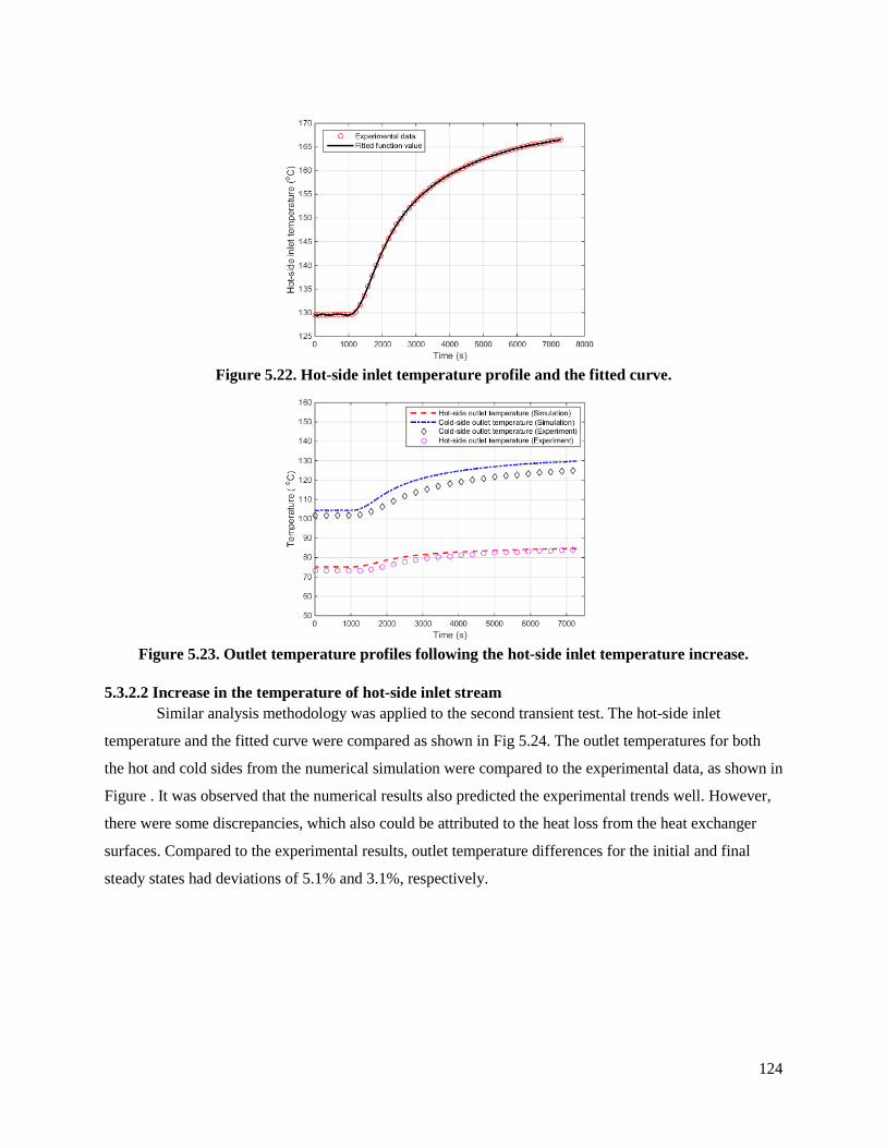
124
Figure 5.22. Hot-side inlet temperature profile and the fitted curve.
Figure 5.23. Outlet temperature profiles following the hot-side inlet temperature increase.
5.3.2.2 Increase in the temperature of hot-side inlet stream
Similar analysis methodology was applied to the second transient test. The hot-side inlet
temperature and the fitted curve were compared as shown in Fig 5.24. The outlet temperatures for both
the hot and cold sides from the numerical simulation were compared to the experimental data, as shown in
Figure . It was observed that the numerical results also predicted the experimental trends well. However,
there were some discrepancies, which also could be attributed to the heat loss from the heat exchanger
surfaces. Compared to the experimental results, outlet temperature differences for the initial and final
steady states had deviations of 5.1% and 3.1%, respectively.
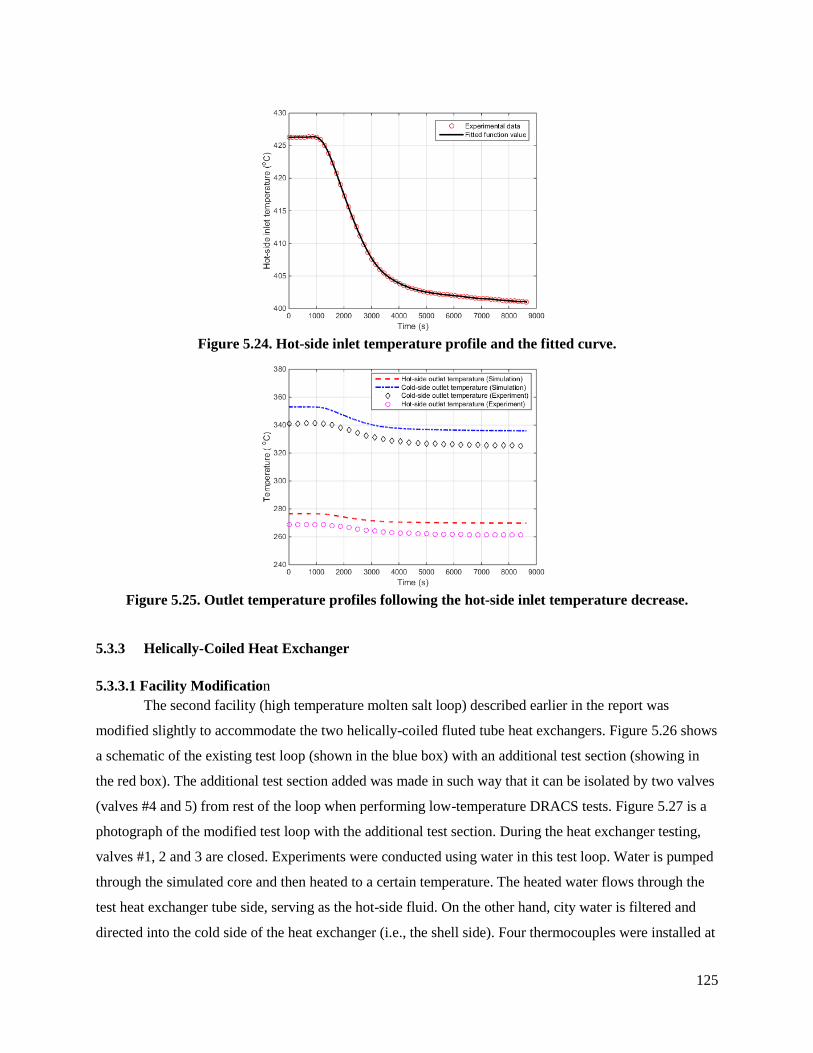
125
Figure 5.24. Hot-side inlet temperature profile and the fitted curve.
Figure 5.25. Outlet temperature profiles following the hot-side inlet temperature decrease.
5.3.3 Helically-Coiled Heat Exchanger
5.3.3.1 Facility Modification
The second facility (high temperature molten salt loop) described earlier in the report was
modified slightly to accommodate the two helically-coiled fluted tube heat exchangers. Figure 5.26 shows
a schematic of the existing test loop (shown in the blue box) with an additional test section (showing in
the red box). The additional test section added was made in such way that it can be isolated by two valves
(valves #4 and 5) from rest of the loop when performing low-temperature DRACS tests. Figure 5.27 is a
photograph of the modified test loop with the additional test section. During the heat exchanger testing,
valves #1, 2 and 3 are closed. Experiments were conducted using water in this test loop. Water is pumped
through the simulated core and then heated to a certain temperature. The heated water flows through the
test heat exchanger tube side, serving as the hot-side fluid. On the other hand, city water is filtered and
directed into the cold side of the heat exchanger (i.e., the shell side). Four thermocouples were installed at
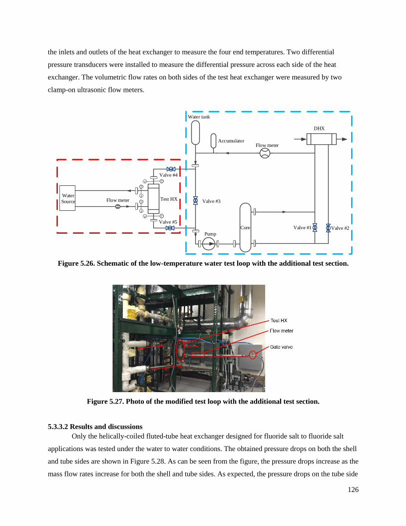
126
the inlets and outlets of the heat exchanger to measure the four end temperatures. Two differential
pressure transducers were installed to measure the differential pressure across each side of the heat
exchanger. The volumetric flow rates on both sides of the test heat exchanger were measured by two
clamp-on ultrasonic flow meters.
Water tank
Core
AccumulatorFlow meter
Pump
Test HX
Tp
T
p
T
p
Tp
DHX
Valve #1 Valve #2
Valve #3
Valve #4
Valve #5
Water
Source Flow meter
Figure 5.26. Schematic of the low-temperature water test loop with the additional test section.
Figure 5.27. Photo of the modified test loop with the additional test section.
5.3.3.2 Results and discussions
Only the helically-coiled fluted-tube heat exchanger designed for fluoride salt to fluoride salt
applications was tested under the water to water conditions. The obtained pressure drops on both the shell
and tube sides are shown in Figure 5.28. As can be seen from the figure, the pressure drops increase as the
mass flow rates increase for both the shell and tube sides. As expected, the pressure drops on the tube side
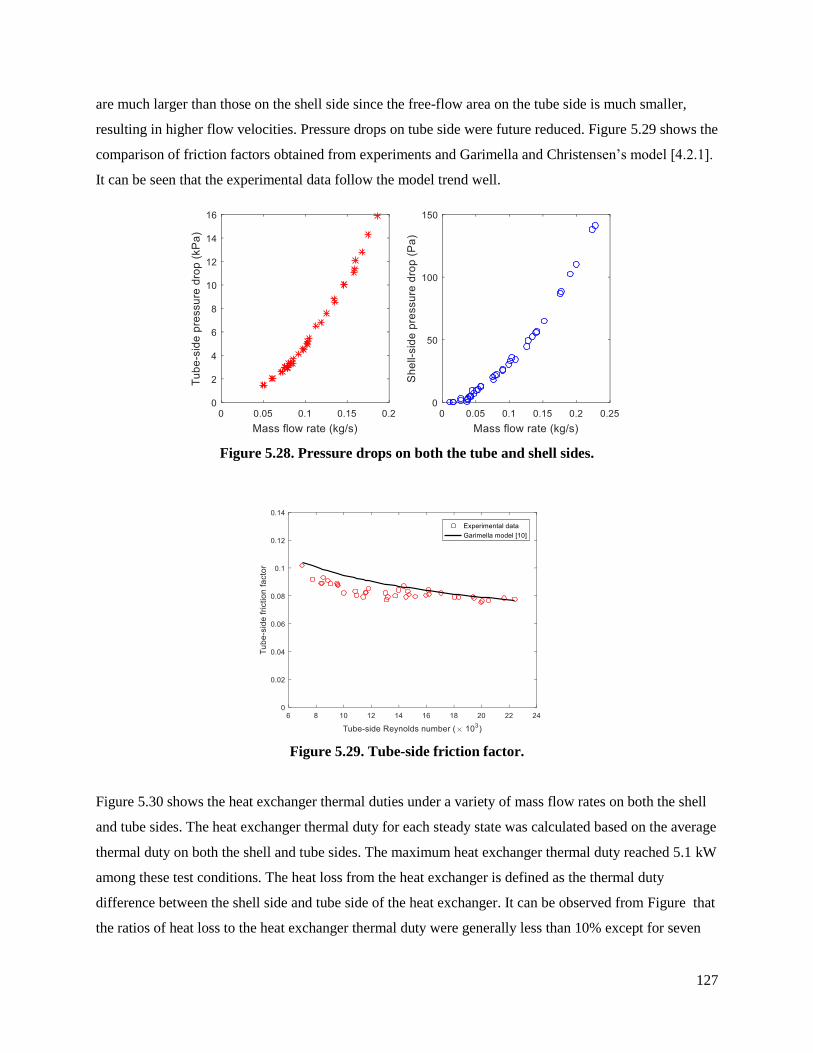
127
are much larger than those on the shell side since the free-flow area on the tube side is much smaller,
resulting in higher flow velocities. Pressure drops on tube side were future reduced. Figure 5.29 shows the
comparison of friction factors obtained from experiments and Garimella and Christensen’s model [4.2.1].
It can be seen that the experimental data follow the model trend well.
Figure 5.28. Pressure drops on both the tube and shell sides.
Figure 5.29. Tube-side friction factor.
Figure 5.30 shows the heat exchanger thermal duties under a variety of mass flow rates on both the shell
and tube sides. The heat exchanger thermal duty for each steady state was calculated based on the average
thermal duty on both the shell and tube sides. The maximum heat exchanger thermal duty reached 5.1 kW
among these test conditions. The heat loss from the heat exchanger is defined as the thermal duty
difference between the shell side and tube side of the heat exchanger. It can be observed from Figure that
the ratios of heat loss to the heat exchanger thermal duty were generally less than 10% except for seven
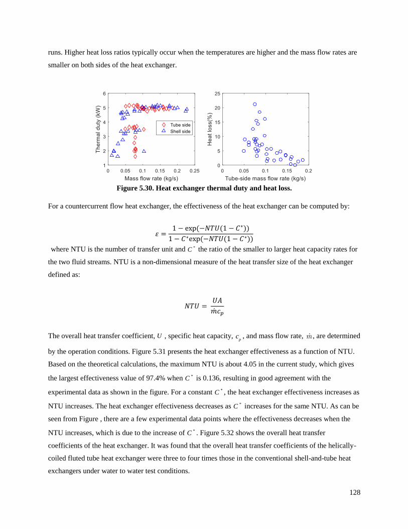
128
runs. Higher heat loss ratios typically occur when the temperatures are higher and the mass flow rates are
smaller on both sides of the heat exchanger.
Figure 5.30. Heat exchanger thermal duty and heat loss.
For a countercurrent flow heat exchanger, the effectiveness of the heat exchanger can be computed by:
𝜀 =1 − exp (−𝑁𝑇𝑈(1 − 𝐶∗))
1 − 𝐶∗exp (−𝑁𝑇𝑈(1 − 𝐶∗))
where NTU is the number of transfer unit and *C the ratio of the smaller to larger heat capacity rates for
the two fluid streams. NTU is a non-dimensional measure of the heat transfer size of the heat exchanger
defined as:
𝑁𝑇𝑈 = 𝑈𝐴
�̇�𝑐𝑝
The overall heat transfer coefficient, U , specific heat capacity, p
c , and mass flow rate, , are determined
by the operation conditions. Figure 5.31 presents the heat exchanger effectiveness as a function of NTU.
Based on the theoretical calculations, the maximum NTU is about 4.05 in the current study, which gives
the largest effectiveness value of 97.4% when *C is 0.136, resulting in good agreement with the
experimental data as shown in the figure. For a constant *C , the heat exchanger effectiveness increases as
NTU increases. The heat exchanger effectiveness decreases as *C increases for the same NTU. As can be
seen from Figure , there are a few experimental data points where the effectiveness decreases when the
NTU increases, which is due to the increase of *C . Figure 5.32 shows the overall heat transfer
coefficients of the heat exchanger. It was found that the overall heat transfer coefficients of the helically-
coiled fluted tube heat exchanger were three to four times those in the conventional shell-and-tube heat
exchangers under water to water test conditions.

129
Figure 5.31. Heat exchanger effectiveness as a function of NTU.
Figure 5.32. Overall heat transfer coefficient of the heat exchanger.
5.4 Summary
Prototype heat exchangers – wavy-channel printed circuit heat exchanger (PCHE) and helically coiled
heat exchanger – were designed and fabricated for the study. These heat exchangers, as well as an
available straight channel heat exchanger were installed in the experimental facilities at The Ohio State
University and subjected to steady-state and dynamic testing. The dynamic tests involved introducing a
process disturbance in terms of a change in temperature or flow rate of a stream (or streams), or a
combination thereof. The response of the system was monitored through changes in the temperatures, and
experimental data analyzed with respect to the thermal hydraulic characteristics. Dynamic models were
also developed for the system and the response simulated by user-developed MATLAB codes. The
simulation results were compared with the experimental data for validating the models. These
comparisons indicate that the models are able to predict the system behavior reasonably well.
130
6. Conclusions
Advanced reactors derive their potential from their ability to provide, in addition to power
generation, high-temperature heat that can be utilized for a variety of process applications including co-
generation, conversion of coal to liquids and formulation of chemical feedstocks. The IHX is a critical
component in the next generation nuclear plant system and an effective design of the IHX is essential for
high efficiency operation. In addition, the transient behavior of IHX and the coupling between the reactor
primary system and the secondary system (power conversion system and process heat application) is
essential to the reactor safety and therefore is critical to regulators for design certification application. The
complexity of the system requires development of advanced modeling and simulation tools to handle the
interaction between the various components of the system during normal and off-normal operations, and
validating the results through experimental observations.
The research conducted in this project has yielded information on the thermal designs and
advanced control strategies for different IHX types for various combinations of coolants and operating
temperatures and conditions. The transient behavior of the reactor-IHX-SHX system was simulated for
various system disturbances, and the effectiveness of the control system to mitigate the adverse impacts of
such events demonstrated clearly. The simulation results were compared with the experimental results,
with the close agreement between the two indicating the validity of the theoretical models developed to
describe the system. These results and information are valuable in understanding the coupled response of
the reactor-IHX-SHX system to various transients and the development of intelligent control systems for
the next generation nuclear reactor systems.
The results of the research have been presented at several national and international meetings of
various professional societies, and published in refereed technical publications. The project has also
resulted in mentoring of several graduate and undergraduate students, with two students graduating with
graduate degrees in chemical and nuclear engineering. The project has thus also served to address the
need for qualified, technical workforce for the nuclear field.

131
References
Al-Dawery, S., Alrahawi, A., Al-Zobai, K., 2012. Dynamic Modeling and Control of Plate Heat
Exchanger. Int. J. Heat Mass Transfer, 55, 6873-6880.
Amin, M.R., Rocco, R., 2006. “Dynamic modeling of a closed loop Brayton cycle for space auxiliary
electric power systems.” Proceedings of 3rd BSME-ASME International Conference of Thermal
Engineering, Dhaka, Bangladesh, December 20-22, 2006.
Arnold, J., Garimella, S., Christensen, R.N., 1990. “A Manual for Heat Exchanger Design using Spirally
Fluted Tubes,” The Ohio State University.
Bartel, N., Chen, M., Utgikar, V., Sun, X., Kim, I.-H., Christensen, R., Sabharwall, P., 2015.
“Comparative analysis of compact heat exchangers for application as the intermediate heat
exchanger for advanced reactors,” Ann. Nucl. Energy, 81, 143-149.
Chapra, S., Canale, R., 2010. “Numerical Methods for Engineers,” sixth ed., McGraw-Hill, New York.
Chen, M., Lv, Q., Kim, I.-H., Sun, X., Christensen, R., Utgikar, V., Sabharwall, P., 2015. “Dynamic
analysis of a fluoride salt-cooled high-temperature reactor coupled to a helium Brayton power
system via an intermediate loop,” Prog. Nucl. Energy, 83, 283-293.
Das, S., Pan, I., Das, A., 2013. “Fractional order fuzzy control of nuclear reactor power with thermal-
hydraulic effects in the presence of random network induced delay and sensor noise having long
range dependence,” Energy Conv. Manage., 68, 200-218.
Galvez, C., 2011. “Design and transient analysis of passive safety cooling systems for advanced nuclear
reactors,” Doctoral dissertation, University of California.
Garimella, S., 1990. “Experimental Investigation of Heat Transfer and Pressure Drop Characteristics of
Annuli with Spirally Fluted Inner Tubes,” Doctoral Dissertation, The Ohio State University.
Garimella, S., Christensen, R.N., 1995a. “Heat Transfer and Pressure Drop Characteristics of Spirally
Fluted Annuli: Part I: Hydrodynamics,” J. Heat Transfer, 117, 54-60.
Garimella, S., Christensen, R.N., 1995b. “Heat Transfer and Pressure Drop Characteristics of Spirally
Fluted Annuli: Part II: Heat Transfer,” Journal of Heat Transfer, 117, 61-68.
Gnielinski, V. 1983. “Forced Convection in Ducts,” in Heat Exchanger Design Handbook, Volume 2,
Hewitt, G.F., Executive Ed., Hemisphere, New York
Guomin, C., Jinyang, W., Tao, J., Xiangbai, H., 2011. Transfer behavior of heat exchanger. Adv. Mater.
Res., 233-235, 1281-1287. doi: 10.4028/www.scientific.net/AMR.233-235.1281.
Heng, X., 2011. “Model Development and Simulation of Transient Behavior of Helium Turbine System,”
Ann. Nuc. Energy, 38, 2797-2805.
Hesselgreaves, J.E., 2001. “Compact Heat Exchangers: Selection, Design and Operation,” Gulf
Professional Publishing.

132
Holcomb, D.E., Cetiner, S.M., Flanagan, G.F., Peretz, F.J., Yoder, G.L., Jr., 2009. “An Analysis of
Testing Requirements for Fluoride Salt-cooled High Temperature Reactor Components,”
ORNL/TM-2009/297, Oak Ridge National Laboratory, November 2009.
Ishizuka, T., Kato, Y. Muto, Y., Nikiting, K., Ngo, T.L.,2006. “Printed Circuit Heat Exchanger Thermal-
Hydraulic Performance in Supercritical CO2 Experimental Loop,” Int. J. Refrig., 29, 807-814.
Jayakumar, J.S., 2013. “Helically Coiled Heat Exchangers” in Heat Exchangers - Basics Design
Applications Edt| InTechOpen, InTech: Open Access Publisher [eBooks]. Retrieved at April 20,
2013, from the website Intech: Open Science | Open Minds at
http://www.intechopen.com/books/heat-exchangers-basics-design-applications
Kakac, S., Liu, H., 2002. “Heat Exchangers: Selection Rating and Thermal Design,” CRC Press, ISBN 0-
8493-0902-6.
Kato, R., Nishihara, T., Kumitomi, K., 2007. “Design of the Intermediate Heat Exchanger for High
Temperature Gas-Cooled Reactor Hydrogen Cogeneration System,” Japanese Nucl. Soc., 692,
141-148.
Kim, E.S., Oh, C.H., and Sherman, S., 2008. Simplified Optimum Sizing and Cost Analysis for Compact
Heat Exchanger in VHTR. Nucl. Eng. Des., 238, 2635-2647.
Kim, I.H., 2012. “Experimental and Numerical Investigations of Thermal-hydraulic Characteristics for
the Design of a Printed Circuit Heat Exchanger (PCHE) in HTGRs,” Doctoral dissertation, Korea
Advanced Institute of Science and Technology.
Koch, 2013. Koch Industries website, http://www.kochheattransfer.com/products/twisted-tube-bundle-
technology
Kim, I.H., No, H.C., 2012. “Physical model development and optimal design of PCHE for intermediate
heat exchangers in HTGRs.” Nucl. Eng. Des., 246, 243-250.
Lamarsh, J., Baratta, A., 2001. “Introduction to Nuclear Engineering,” third ed., Prentice Hall, Upper
Saddle River.
Losier, C.R.D., Subramanian, S., Ponyavin, V., Chen, Y., Hechanova, A.E., Peterson, P.F., 2007. “The
Parametric Study of an Innovative Offset Strip-Fin Heat Exchanger,” J. Heat Trans., 129, 1453-
1458.
Manglik, R.M., Bergles, A.E., 1995. “Heat Transfer and Pressure Drop Correlations for the Rectangular
Offset Strip Fin Compact Heat Exchanger,” Exper. Thermal Fluid Sci., 10, 171-180.
Mylavarapu, S., Sun, X., R.R., Glosup, R.E., and Patterson, M.W., 2011, “Fabrication and Design
Aspects of High-Temperature Compact Diffusino Bonded Heat Exchangers,” Nucl. Eng. Des.,
published on-line, doi:10.1016/j.nucengdes.2011.08.043.

133
Mylavarapu, S.K., 2011. “Design, Fabrication, Performance Testing, and Modeling of Diffusion Bonded
Compact Heat Exchangers in a High-temperature Helium Test Facility,” Doctoral dissertation,
The Ohio State University.
Oh, C.H., Kim, E.S., 2008. Heat Exchanger Design Options and Tritium Transport study for the VHTR
System, INL/EXT-08-14799, Idaho National Laboratory, Idaho Falls, ID.
Ragheb, M., 2013. “Loss of coolant accident, LOCA,” University of Illinois at Urbana-Champaign, IL.
Sabharwall, P., Patterson, M., Utgikar, V., Gunnerson, F., 2010. Phase change heat transfer device for
process heat application. Nucl. Eng. Des., 240, 2409-2414.
Sabharwall, P., Utgikar, V., Tokuhiro, A., Gunnerson, F., 2009. Design of liquid metal phase change heat
exchanger for next generation nuclear plant process heat application. J. Nucl. Sci. Technol., 46(6),
534-544.
Silaipillayarputhur, K., Idem, S., 2011. Step Response of a Single-Pass Crossflow Heat Exchanger with
Variable Inlet Temperatures and Mass Flow Rates. ASME 2011, Denver, Colorado, November 11-
17, 2011, International Mechanical Engineering Congress & Exposition.
Smith, E.M., 2005. “Advances in Thermal Design of Heat Exchangers: A Numerical Approach,” Wiley,
England.
Srinivasan, V., 1993. “Experimental and numerical investigation of heat transfer and pressure drop in
flow through spirally fluted tubes.” Doctoral dissertation, The Ohio State University.
Techo, R., Tiekner, R.R., James, R.E., 1965. An Accurate Equation for the Computation of the Friction
Factor for Smooth Pipes for the Reynolds Number. J. Appl. Mech., 32, 443.
Wenlong, L., Heng, X., Zuoyi, Z., Yujie, D., 2012. “Development and primary verification of a transient
analysis software for high temperature gas-cooled reactor helium turbine power system,” Nuc.
Eng. Des., 250, 219-228.
Williams, D.F., Toth, L.M., Clarno K.T., 2006. “Assessment of Candidate Molten Salt Coolants for the
Advanced High-Temperature Reactor (AHTR),” ORNL.TM-2006/12, Oak Ridge National
Laboratory, Oak Ridge, TN.
Wright, S.A., Vernon, M.E., Pickard, P.S., 2006. “Concept design for high temperature helium Brayton
cycle with interstage heating and cooling.” Sandia National Laboratories.
Zukauskas, A.A., Kakac, S., Shah, R.K., and Aung, W., 1987. “Convective Heat Transfer in Cross Flow,”
in Handbook of Single-Phase Convective Heat Transfer, Eds., John Wiley & Sons, New York,
Ch. 5.
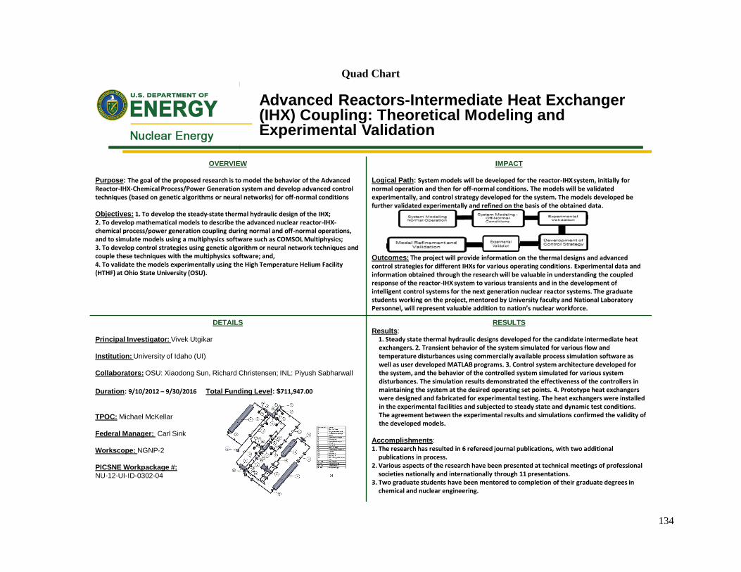
134
Quad Chart
OVERVIEW
Purpose: The goal of the proposed research is to model the behavior of the Advanced Reactor-IHX-Chemical Process/Power Generation system and develop advanced control techniques (based on genetic algorithms or neural networks) for off-normal conditions
Objectives: 1. To develop the steady-state thermal hydraulic design of the IHX;2. To develop mathematical models to describe the advanced nuclear reactor-IHX-chemical process/power generation coupling during normal and off-normal operations, and to simulate models using a multiphysics software such as COMSOL Multiphysics;3. To develop control strategies using genetic algorithm or neural network techniques and couple these techniques with the multiphysics software; and,4. To validate the models experimentally using the High Temperature Helium Facility (HTHF) at Ohio State University (OSU).
IMPACT
Logical Path: System models will be developed for the reactor-IHX system, initially for normal operation and then for off-normal conditions. The models will be validated experimentally, and control strategy developed for the system. The models developed be further validated experimentally and refined on the basis of the obtained data.
Outcomes: The project will provide information on the thermal designs and advanced control strategies for different IHXs for various operating conditions. Experimental data and information obtained through the research will be valuable in understanding the coupled response of the reactor-IHX system to various transients and in the development of intelligent control systems for the next generation nuclear reactor systems. The graduatestudents working on the project, mentored by University faculty and National Laboratory Personnel, will represent valuable addition to nation’s nuclear workforce.
DETAILS
Principal Investigator: Vivek Utgikar
Institution: University of Idaho (UI)
Collaborators: OSU: Xiaodong Sun, Richard Christensen; INL: Piyush Sabharwall
Duration: 9/10/2012 – 9/30/2016 Total Funding Level: $711,947.00
TPOC: Michael McKellar
Federal Manager: Carl Sink
Workscope: NGNP-2
PICSNE Workpackage #:
NU-12-UI-ID-0302-04
RESULTS
Results: 1. Steady state thermal hydraulic designs developed for the candidate intermediate heat exchangers. 2. Transient behavior of the system simulated for various flow and temperature disturbances using commercially available process simulation software as well as user developed MATLAB programs. 3. Control system architecture developed for the system, and the behavior of the controlled system simulated for various system disturbances. The simulation results demonstrated the effectiveness of the controllers in maintaining the system at the desired operating set points. 4. Prototype heat exchangers were designed and fabricated for experimental testing. The heat exchangers were installed in the experimental facilities and subjected to steady state and dynamic test conditions. The agreement between the experimental results and simulations confirmed the validity of the developed models.
Accomplishments: 1. The research has resulted in 6 refereed journal publications, with two additional
publications in process.2. Various aspects of the research have been presented at technical meetings of professional
societies nationally and internationally through 11 presentations.3. Two graduate students have been mentored to completion of their graduate degrees in
chemical and nuclear engineering.
Advanced Reactors-Intermediate Heat Exchanger (IHX) Coupling: Theoretical Modeling and Experimental Validation