advanced finite-difference methods for seismic...

GEOHORIZONS December 2009/5

Advanced finite-difference methods for seismic modelingYang Liu1,2 and Mrinal K Sen2

1State Key Laboratory of Petroleum Resource and Prospecting (China University of Petroleum, Beijing), Beijing, 102249, China2The Institute for Geophysics, John A. and Katherine G. Jackson School of Geosciences, The University of Texas at Austin, 10100

Burnet Road, R2200 Austin, TX 78758, USAE-mail: [email protected], [email protected]

variable time step (Tessmer, 2000) and implicit methods(Emerman et al, 1982; Zhang and Zhang, 2007).

One obvious approach to improve on the accuracyof FD calculation is to design high order operators forcomputing the derivatives (Dablain, 1986; Fornberg, 1987;Crase, 1990; Liu et al, 1998; Dong, 2000; Pei, 2004; Chen,2007; Liu et al, 2008; Liu and Sen, 2009). In this paper, wereview the developments of arbitrary even-order FDMs forseismic modeling, including EFDMs (explicit FDMs), IFDMs(implicit FDMs) and time-space domain FDMs.

First, we briefly review the seismic wave equations,finite difference, dispersion, stability and the necessity ofhigh-order finite differences. We restrict our discussion toacoustic wave equation because of the ease of algebra. Theseare followed by description of EFDMs, new IFDMs and time-space domain FDMs. Finally, we show some numericalexamples to demonstrate the salient features of differentalgorithms.

Background

Seismic wave equations: finite differenceapproximations

Seismic wave equations, used to describe seismicwave propagation in the subsurface, are typically partialdifferential equations containing spatial and temporalderivatives. The constant density acoustic wave equationhas been used most widely in seismic modeling, migration

Introduction

The finite-difference method (FDM), one of the mostpopular methods of numerical solution of partial differentialequations, has been widely used in seismic modeling (e.g.,Kelly et. al., 1976; Virieux, 1986; Igel et. al. 1995; Etgen, 2007;Bansal and Sen, 2008) and migration (Claerbout, 1985; Li,1991; Zhang et. al., 2000; Fei et. al. 2008). The development ofan FD operator is based generally on a Taylor seriesrepresentation of a function (the wavefield) resulting in aformulation for numerical evaluation of the derivativesappearing in the wave equation. The accuracy of theseoperators is dependent on the order of approximation, namely,the number of terms used in the Taylor series representationof the function. Thus a discrete version of the wave equationis derived where the wavefield is propagated starting fromthe source location (the initial condition). In general, accuracyof the derivative calculation for a given order depends ongrid spacing. A small grid size helps to increase the accuracybut results in a large number of grids to represent a geologicmodel. Thus, there is a substantial increase in memory andfloating point operations making these methods prohibitivefor realistic modeling of complex geological structures in theseismic frequency range.

To improve the accuracy and stability of a FDM innumerical modeling, many methods have been developedincluding difference schemes of variable grid (Wang et. al.,1996; Hayashi et. al., 1999), irregular grid (Opršal et. al., 1999),standard staggered grid (Virieux, 1986; Levander, 1988;Robertsson et al., 1994; Graves, 1996), rotated staggered grid(Gold et al., 1997; Saenger et. al., 2004; Bohlen et. al., 2006),

Abstract

The finite-difference methods (FDMs) have been widely used in seismic modeling and migration. In this paper,we review the conventional arbitrary-order explicit FDMs and their recent developments, including arbitrary even-orderimplicit FDMs for standard grids and arbitrary even-order time-space domain FDMs for acoustic wave equations. Fora given accuracy, an arbitrary even-order FDM can provide a trade-off between the order number and grid size. Theseexplicit FDMs are the most popular in seismic modeling community. The finite-difference methods that are implicit inspace are not very common because they generally require more computer resources than the explicit FDMs. Here weshow that a new class of implicit FDMs can be derived that require solving a tri-diagonal system, which makes theresulting algorithm computationally very efficient. Therefore, some high-order explicit FDM may be replaced by animplicit FDM of some order to decrease the computation time without affecting the accuracy. We further demonstratethat we can also derive the FD coefficients in the joint time-space domain. These high-order spatial finite-differencestencils designed in joint time-space domain, when used in acoustic wave equation modeling, can provide even greateraccuracy than those designed in the space domain alone under the same discretization. We demonstrate performance ofthese algorithms using some realistic 2D numerical examples.


and inversion. The 1D acoustic wave equation in ahomogenous medium is given by

,

………..(1)

where,

is a scalar wave field, and is the velocity.

From Equation (1), we can see that the wave field isa function of the spatial coordinate and time.

The following 2nd-order finite difference is usuallyused for calculating temporal derivatives,

, ………..(2)

where,

, ………..(3)

h and τ are grid size and time step respectively (see Figure 1).For the 2nd-order continuous-time wave field,

. ………..(4)

Thus, a smaller time step leads to greater accuracy forcomputing temporal derivatives. Higher order approximationof Equation (2) can also be derived from the Taylor series.Note that Equation (2) requires the wavefield values at thecurrent time step, past time step and a future time step at agiven spatial point. Such a scheme is called an explicit schemein time. Generally, an explicit high-order finite difference onthe temporal derivatives requires large computer memory andis usually unstable. An equation similar to Equation (2) canalso be derived for a spatial derivative which will require the

Fig.1 Illustration of grids for wave fields in the time-space domain

wavefield values at the current grid and its two neighboringgrids, at a given time step. Such a scheme is called an explicitscheme in space. However, unlike the temporal derivatives, ahigh-order finite difference on the spatial derivatives is stable.A (2N)th-order finite difference formula for the 2nd-orderspatial derivative is given by

, ……....(5)

where, are the finite-difference coefficients and theirexpressions are given in the following section. When ,we can obtain , , then Equation (5) is similar toEquation (2). When , then , , .Also, a smaller grid size can help attain greater accuracy forspatial derivatives.

Substituting Equations (2) and (5) into Equation (1), we have

.

………..(6)

Rearranging Equation (6), we obtain,

,

………..(7)

where, r = vτ/h. Equation (7) is the recursion formula forsolving 1D wave equation by a finite-difference method. Therecursion begins with the wave field values known at twosuccessive time steps t=0 and t=τ. The wavefield values at afuture time step at all the spatial locations are computed usingEquation (7).

Dispersion

One obvious observation we can make is thattruncation of terms in a Taylor series expansion causesinaccuracies in the evaluation of a derivative. It also causesfrequency-dependent numerical errors due to truncation ofhigher order terms, even when the material properties are notfrequency dependent. In fact, we observe a numericalphenomenon called ‘dispersion’ that is similar to what isobserved in dissipative or attenuating media in whichpropagation velocities are frequency-dependent. Frequency-dependent numerical dispersion is observed even in non-attenuating media due to inadequate sampling of wavefieldsin space and time.

Here, we discuss the dispersion generated by therecursion formula (7). Using a plane wave theory, we let


, ………..(8)

where, k is the wavenumber, ω is the angular frequency, and. Substituting Equation (8) into (7) and simplifying

it, we have

, ………..(9)

which can be solved for a frequency ω; a group velocity isgiven by the ratio of frequency ω to wavenumber k. Thegroup or dispersion velocity is

.

………..(10)

Note that, is the velocity with which the wavepropagates through numerical grids. This expression showsthat the dispersion velocity depends on the medium velocity

, grid size , time step , wavenumber and finite-differentcoefficients .

Using Equation (10) and r = vτ/h, we define aparameter δ to describe the dispersion

………..(11)

Note that the parameter is the ratio of dispersionvelocity to the true velocity of the medium and in fact it is ameasure of numerical error of finite difference approximation.If equals 1, there is no dispersion. If is far from 1, a largedispersion will occur. Thus our primary goal is to make close to 1 by a proper choice of grid spacing for a given

velocity and frequency. Since is equal to at the Nyquistfrequency, only ranges from 0 to when calculating .

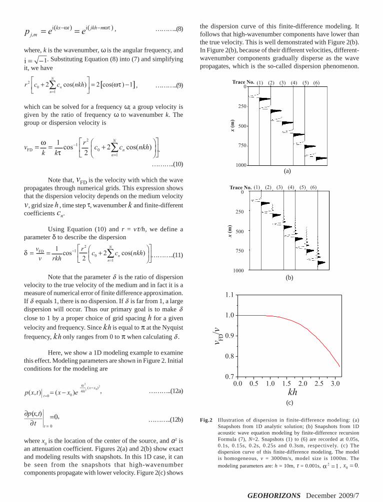
Here, we show a 1D modeling example to examinethis effect. Modeling parameters are shown in Figure 2. Initialconditions for the modeling are

, ………..(12a)

………..(12b)

where x0 is the location of the center of the source, and α2 is

an attenuation coefficient. Figures 2(a) and 2(b) show exactand modeling results with snapshots. In this 1D case, it canbe seen from the snapshots that high-wavenumbercomponents propagate with lower velocity. Figure 2(c) shows

the dispersion curve of this finite-difference modeling. Itfollows that high-wavenumber components have lower thanthe true velocity. This is well demonstrated with Figure 2(b).In Figure 2(b), because of their different velocities, different-wavenumber components gradually disperse as the wavepropagates, which is the so-called dispersion phenomenon.

Fig.2 Illustration of dispersion in finite-difference modeling: (a)Snapshots from 1D analytic solution; (b) Snapshots from 1Dacoustic wave equation modeling by finite-difference recursionFormula (7), N=2. Snapshots (1) to (6) are recorded at 0.05s,0.1s, 0.15s, 0.2s, 0.25s and 0.3sm, respectively. (c) Thedispersion curve of this finite-difference modeling. The modelis homogeneous, v = 3000m/s, model size is 1000m. The

modeling parameters are: h = 10m, τ = 0.001s, , .

(c)

(b)

(a)


(b)

Stability

Recursion formula, such as the one used in Equation(7), is commonly used to perform finite-difference modeling.If the modeling parameters are inappropriate, for example, iftime step is too large, the recursion will be unstable. In otherwords, the wavefield will grow and will eventually exceed themachine precision.

We will now use a conventional eigenvalue method(Chen and Guan, 1989) of stability analysis to derive thestability condition for recursion formula (7). Let

.

………..(13)

According to Equation (7) and (13), we can obtain(see Appendix A)

, ………..(14)

where G is a transition matrix,

. ………..(15)

When the absolute values of the transition matrixeigenvalues are less than or equal to 1, the recursion is stable.

If , the roots of the eigenvalue equation will be less than or equal to 1. Then, the following stabilitycondition can be obtained

, ………..(16)

where, N1 =int [(N+1)/2] and int is a function to get the integer

part of a value. We calculate the variation of s with N, which isshown in Figure 3. From this figure, we can see that the area ofr for stable recursion decreases with the increase of N.

Necessity of high-order finite differences on thespatial derivatives

In the previous section, we demonstrated the presenceof grid dispersion in the acoustic wavefield modeled by a 2nd-order finite-difference operator. There are several ways toreduce the dispersion. The first way is to decrease the gridsize. Due to the limitation of computer memory, we cannot usea very small grid size, especially for 3D modeling. The secondapproach is to decrease the time step. Figure 4(a) showsdispersion curves of low-order finite-difference modeling fordifferent time steps, which suggest that decreasing the timestep will decrease the dispersion of low-wavenumbercomponents, but will not decrease the dispersion of middle-and high-wavenumber components. The third approach is touse high-order finite differences. Figure 4(b) shows dispersioncurves for high-order finite-difference modeling for differenttime steps, which suggest that decreasing time step willdecrease the dispersion of low- and middle-wavenumbercomponents. Comparing Figure 4(a) with 4(b), we concludethat a high-order finite difference on the spatial derivatives isnecessary to reduce dispersion. One other approach tosuppress the grid dispersion is to use staggered grids (e.g.,Virieux, 1986; Kindelan et al 1990; Graves, 1996; Saenger andBohlen, 2004; Bohlen and Saenger; 2006). However, in thispaper we will discuss standard grids only.

Fig.3 Illustration of stability condition of 1D acoustic wave equationmodeling by finite-difference recursion Formula (7). Therecursion is stable when .

Fig. 4 Dispersion curves for 1D acoustic wave equation modeling byfinite-difference recursion Formula (7) for different time steps.v = 3000m/s, h = 10m. (a) Low-order finite difference onspatial derivatives, N=2; (b) High-order finite difference onspatial derivatives, N=10.

(a)


Explicit finite-difference methods

Centered finite-difference formulas in a standard gridscheme are usually used to numerically solve partialdifferential equations, which generally involve the first-orderand the second-order derivatives in a seismic modelingapplication. In the following, we introduce centered finite-difference formulas with arbitrary even-order accuracy forthe first-order and the second-order derivatives.

Explicit finite-difference formula for the 1st-orderderivatives

A (2N)th-order finite-difference formula for the first-orderderivatives can be expressed as (Dablain, 1986)

, …............(17)

where, p(x) is a function of x, x is a real variable, h is a smallconstant value of grid size, N is a positive integer; the finite-difference coefficient c

n is an odd discrete sequence. Appendix

B gives a methodology based on plane wave theory forderiving finite-difference coefficients. c

n can be computed

by the following formula (Fornberg, 1987; Liu et. al., 1998,2008; Liu and Sen, 2009a)

. .……..(18)

When ,

. .………..(19)

Thus, there exists a limit at which we can attaininfinite accuracy theoretically and at this limit we arrive at thepseudospectral method (Fornberg, 1987).

Explicit finite-difference formula for the 2nd-orderderivatives

A (2N)th-order finite-difference formula for thesecond-order derivatives can be expressed as

, .………..(20)

where, the difference coefficient, cn an even discrete sequence,

can be computed by the following formulas (Liu et. al., 1998,2008; Liu and Sen, 2009a)

……..(21)

When ,

. . .………..(22)

To examine the accuracy of these finite-differenceformulas (17) and (20), the following expressions are used(Liu and Sen, 2009a)

, . .………..(23a)

, . .………..(23b)

where, , k is wavenumber. When calculating thevalues of the above expressions, α only ranges from 0 to π/2because kh is equal to π at the Nyquist frequency. Thecalculated values from formulas (23a) and (23b) are comparedwith the exact values of α for different order numbersdetermined by N, shown in Figure 5. We notice that the

Fig. 5 Accuracy of explicit finite-difference formulas(a) The exact α and f

1(α )of EFDM with different order

numbers for the first-order derivatives(b) The exact α and f

2(α) of EFDM with different order numbers

for the second-order derivatives

(b)

(a)

.


accuracy increases with the increase of the order number.

Implicit finite-difference methods

We noted in the previous section that an EFDMdirectly calculates the derivative value at some point usingthe function values at that point and at its neighboring points.However, an IFDM (implicit FDM) expresses the derivativevalue at some point in terms of the function values at thatpoint and at its neighboring points and the derivative valuesat its neighboring points. For example, a compact finite-difference method (CFDM) is one such IFDM (Lele 1992).However, IFDMs are usually considered expensive due tothe requirement of solving a larger number of equations andare therefore not very popular. Liu and Sen (2009a) derivednew implicit formulas for space derivatives with arbitraryeven-order accuracy for arbitrary-order derivatives. Theirapproach requires solving tridiagonal matrix equations only.They also showed that a high-order explicit method may bereplaced by an implicit method of some order, which willincrease the accuracy but not the computational cost.

We first introduce Claerbout’s idea (Claerbout 1985)upon which the methods of Liu and Sen (2009a) are developed.The 2nd-order difference operator for a function is expressed as

. ………..(24).

The accuracy of finite difference can be improvedby adding higher-order terms, that is,

, ………..(25).

where b is an adjustable constant. This expression is rarelyused – it can be changed to the following form (Claerbout 1985)

. ………..(26).

This equation has greater accuracy than equation (24).In order to use the above representation of the 2nd- orderdifference operator, one needs to multiply the FD equationthrough out by the denominator and then rearrange terms tosolve for the unknown.

Implicit finite-difference formula for the 1st-orderderivatives

Motivated by Formula (26), an implicit finite-difference formula for the first-order derivatives can beexpressed as (Liu and Sen, 2009a)

, ………..(27).

where, the difference operator in the denominator is a 2nd-order centered finite difference stencil, , an odd discretesequence, and b can be computed by solving the followingequations (Liu and Sen, 2009a)

…....(28)

Implicit finite-difference formula for the 2nd-orderderivatives

An implicit finite-difference formula for the second-order derivatives can be expressed as (Liu and Sen, 2009a)

, ……….. (29).

where, cn is an even discrete sequence, ,

and b can be computed by solving thefollowing equations (Liu and Sen, 2009a)

……….. (30)

The following expressions are respectively used toexamine the accuracy of implicit finite-difference formulas(27) and (29) (Liu and Sen, 2009a)

, ……….. (31a)

. ……….. (31b)

.

.


The exact values of the above expressions are α ,and the calculated values are compared with α for differentorder numbers determined by N, shown in Figure 6. We cansee that the accuracy increases with the increase of the ordernumber. Comparing Figure 5 with Figure 6, we note that forthe same order number, the accuracy of the implicit method isbetter than that of the corresponding explicit method. It hasbeen found (Liu and Sen, 2009a) that for standard-grid finitedifferences, the accuracy of a (2N+2)th-order implicit formula(27) is nearly equivalent to that of a (6N+2)th-order explicitformula (17) for the first-order derivative, and a (2N+2)th-order implicit formula (29) is nearly equivalent to a (4N+2)th-order explicit formula (20) for the second-order derivative.Because the computation cost of a (2N+2)th-order IFDM isequal to that of an EFDM of some order plus that of solvingtridiagonal equations, a high-order EFDM may be replacedby an IFDM of some order, which will increase the accuracybut not the cost of computation.

Time-space finite-difference methods

In the previous sections, we derived finite-differencestencils of time and space derivatives by using the planewave theory and the truncated Taylor series in time and space

(a) Exact α and g1(α) of IFDM with different order

numbers for the first-order derivative

Fig. 6 Accuracy of implicit finite-difference formulas

(b) Exact α and g2(α) of IFDM with different order

numbers for the second-order derivative

respectively. The finite-difference coefficients are derivedindependently for time and space derivative operators andthe approximations are incorporated into wave equations toarrive at a finite difference based recursion operator.Alternatively, we can apply finite difference approximationof time and space derivatives directly to the wave equationssimultaneously and then derive the coefficients.

To demonstrate this, we start with 1D acoustic waveequation in homogenous media given by Equation (1). A 2nd-order finite difference on the time derivatives, given byEquation (2) is usually used. Generally, the modeling accuracyis improved by using a high-order finite difference on thespatial derivatives; a (2N)th-order finite-difference formula isgiven by Equation (5).

Substituting Equations (2) and (5) into Equation (1)and rearranging, we have

.

……….. (32)

In the conventional method, the finite-differencecoefficients of the space derivatives are determined in thespace domain alone and can be determined by Equation (21)to satisfy Equation (5). It can be proved that when we use the(2N)th-order space domain finite-difference and the 2nd-ordertime domain finite-difference stencils to solve the 1D acousticwave equation, the accuracy order is 2. Obviously, theconclusion is the same for the 2D and 3D acoustic waveequations. It is worthwhile to note that increasing N maydecrease the magnitude of the finite-difference error but maynot increases the accuracy order. The main reason is that thefinite-difference stencils are designed in the space and timedomains separately, but the wave equation must be solved inboth the space and time domains simultaneously.

To address this issue, i.e., not to satisfy Equation(5) but to satisfy Equation (32), a unified methodology(Finkelstein and Kastner, 2007) has been proposed to derivethe finite-difference coefficients in the joint time-spacedomain. The key idea of this method is that the dispersionrelation is completely satisfied at some designatedfrequencies. Thus several equations are formed and the finite-difference coefficients are obtained by solving theseequations simultaneously. It is obvious that there is nodispersion at these designated frequencies when thesecoefficients are used in modeling. However, since differentspecific frequencies give different results and dispersion atother frequencies is not easily controlled, this method maynot be very useful in practice.

Liu and Sen (2009b) developed a new method similarto Finkelstein and Kastner (2007) which employs a plane wavetheory and the Taylor series expansion of dispersion relationto derive the finite-difference coefficients in the joint time-space domain for acoustic wave equation. Using the approach


of Liu and Sen (2009b), the following finite-differencecoefficients are obtained

………..(33)

where, r = ντ/h. When r = 0 , the finite-difference coefficientsare the same as Equation (21). That is, the conventionalmethod is just a special case of the new method. The 1Dfinite-difference modeling method by using these newcoefficients from Equation (33) can reach (2N)th-orderaccuracy.

A parameter δ is defined as follows to describe thedispersion of 1D finite-difference modeling

. ………..(34)

If δ equals 1, there is no dispersion. If δ is far from 1, alarge dispersion will occur. Because kh is equal to π at the Nyquistfrequency, kh only ranges from 0 to π when calculating δ.

Figure 7 shows the variation of the dispersionparameter δ with kh for different space point numbers. Theinvolved parameters are listed in the figure. This figuredemonstrates that

❖ Dispersion decreases with the increase of N.❖ For the conventional method, δ nearly equals 1 when

. The area where δ nearly equals 1 does notextend with the increase of N. That is, increasing Ndecreases the magnitude of the dispersion error butdoes not increase the accuracy order.

❖ For the new method, the area where δ nearly equals 1obviously extends with the increase of N.

❖ The accuracy of the new method is greater than thatof the conventional method.

As an example, the initial conditions of Equations

12(a) and 12(b) are used to perform modeling. Figure 8 showsthe records for different velocities. The dispersion of thenew method with finite-difference coefficients determined byEquation (33) is smaller than that of the conventional methodfinite-difference coefficients determined by Equation (5). Thevariation of the velocity affects the results of the conventionalmethod more than the new method because the finite-difference coefficients of the new method depend on velocity.

(a) Conventional method

(b) New methodFig. 7 1D dispersion curves of the conventional and new methods

for different space point numbers 2N+1, N = 2, 4, 10, 20, v =3000m/s, τ = 0.001s, h = 10m.

Fig. 8 1D modeling records by conventional EFDM and new time-space domain EFDM for different velocities. (1), (4) and (7)are analytic solutions; (2), (5) and (8) are modeling resultsfrom the conventional method, (3), (6) and (9) are modelingresults from the new method. Distances between source centerand these three receivers are 100m, 350m and 600mrespectively. α2 = 2, h = 10m, τ = 0.001s, N = 20.

(a) v = 4500m/s

(b) v = 5500m/s


This new time-space domain method has beenextended to solve 2D acoustic wave equation and can reach(2N)th-order accuracy along 8 directions (Liu and Sen, 2009c).

Numerical modeling examples

To demonstrate the effects of different finite-difference methods stated in this paper, we perform numericalmodeling of 2D acoustic wave equation for the SEG/EAGEsalt model using the following 2D acoustic wave equation

. ………..(35)

In the modeling algorithm, temporal derivatives arediscretized by second-order finite difference similar toEquation (2). Spatial derivatives are discretized by followingthree finite-difference methods discussed earlier. The firstmethod is a conventional 14th-order EFDM; its discretizationformula is given in Equation (20) and the finite-differencecoefficients are determined by Equations (21). The secondone is a 14th-order IFDM; its discretization formula is givenin Equation (29) and the coefficients are determined byEquations (30). The third one is a 28th-order time-spacedomain FDM; its discretization formula is given in Equation(20) and the coefficients are determined in the joint time-space domain (Liu and Sen, 2009c). It has been reported thatthe 14th-order IFDM is nearly equivalent to the conventional28th-order EFDM (Liu and Sen, 2009a).

The SEG/EAGE salt model is shown in Figure 9(a);some modeling parameters are given in the caption of Figure9. Here, we simply extend the model spatially to avoidreflections from the top and other edges of the model. Themodeling snapshots are shown in Figures 9(b), 9(c) and 9(d).The modeling records are shown in Figures 9(e), 9(f) and9(g). Partially enlarged views of these three figures are shownin Figures 9(h), 9(i) and 9(j). Comparing these modeling results,we can see that the accuracy of the 14th-order IFDM is greaterthan that of the conventional 14th EFDM. The 28th-ordertime-space domain FDM can retain the waveform better thanthe conventional 28th-order EFDM or the 14th-order IFDM.

(a) SEG/EAGE salt model

(b) Snapshot computed by the conventional 14th-orderEFDM

(c) Snapshot computed by the 14th-order IFDM (equivalentto the conventional 28th-order EFDM)

(d) Snapshot computed by the 28th-order time-spacedomain FDM

(e) Seismograms by the conventional 14th-order EFDM


Fig.9 Numerical modeling results of 2D acoustic wave equation forthe SEG/EAGE salt model by the conventional 14th EFDM,the 14th-order IFDM (equivalent to conventional 28th-orderEFDM) and the 28th-order time-space domain FDM.τ = 0.002s, h = 20m. The coordinate of the source is (6000m,20m). A one-period sine function with 20Hz frequency is usedas the source wavelet. Time of snapshots is 1600ms.

(f) Seismograms computed by the 14th-order IFDM(equivalent to the conventional 28th-order EFDM)

(g) Seismograms computed by the 28th-order time-spacedomain FDM

(h) Zoom of (e)

(i) Zoom of (f)

(j) Zoom of (g)

Conclusions

The finite difference methods for seismic wavefieldmodeling and imaging are considered to be the most accuratesince these methods are capable of computing all the wavemodes. In addition there is no restriction on the complexityof a geologic model as long as we can represent the model ina discrete form. However, these methods indeed suffer fromnumerical inaccuracy resulting from approximating aderivative operator and discretization of a geologic model.Novel finite-difference operators can be derived to addressthis issue. In this paper, we have reviewed the developmentsof arbitrary even-order FDMs with application to acousticwave equation. The accuracy of these methods increaseswith the increase of order number. Since the accuracy isdetermined by the order number and grid size, arbitrary even-order FDMs can provide a trade-off between the order numberand grid size for a given accuracy. The IFDMs require solvingtridiagonal matrix equations only. Some high-order EFDMmay be replaced by an IFDM of some order to decrease thecomputation time and retain the accuracy. High-order spatialFD stencils designed in the joint time-space domain canimprove the accuracy further for acoustic wave equationmodeling. This time-space domain method can be extendedto solve not only the acoustic wave equation but also othersimilar partial difference equations.

Acknowledgements

Liu would like to thank China Scholarship Council fortheir financial support for this research and UTIG for providingwith the facilities. This research is also partially supported byNSFC under contract No. 40839901 and the National “863”Program of China under contract No. 2007AA06Z218.


References

Bansal, R., and M. K. Sen, 2008, Finite-difference modelling of S-wave splitting in anisotropic media: GeophysicalProspecting, 56, 293-312.

Bohlen, T., and E. H. Saenger, 2006, Accuracy of heterogeneousstaggered-grid finite-difference modeling of Rayleigh waves:Geophysics, 71, T109–T115.

Chen, J., 2007, High-order time discretizations in seismic modeling:Geophysics, 72, SM115–SM122.

Chen J. F., and Guan Z., 1989, Numerical solution of partialdifferential equations, Tsinghua University Press, Beijing,China

Claerbout, J. F., 1985, Imaging the earth’s interior: BlackwellScientific Publications, Inc., Palo. Alto, CA, USA

Crase E., 1990, High-order (space and time) finite-differencemodeling of the elastic wave equation: 60th AnnualInternational Meeting, SEG, Expanded Abstracts, 987-991.

Dablain, M. A., 1986, The application of high-order differencing tothe scalar wave equation: Geophysics, 51, 54–66.

Dong L. G., Z T Ma, et. al., 2000, A staggered-grid high-orderdifference method of one-order elastic wave equation: ChineseJournal of Geophysics, 43: 411-419.

Emerman, S., W. Schmidt, and R. Stephen, 1982, An implicit finite-difference formulation. of the elastic wave equation:Geophysics, 47, 1521-1526.

Etgen, J. T., and M. J. O’Brien, 2007, Computational methods forlarge-scale 3D acoustic finite-difference modeling: A tutorial:Geophysics, 72, SM223–SM230.

Fei, T., and C. L. Liner, 2008, Hybrid fourier finite difference 3Ddepth migration for anisotropic media: Geophysics, 73, S27-S34.

Fornberg, B., 1987, The pseudospectral method - comparisonswith finite differences for the elastic wave equation:Geophysics, 52, 483-501.

Gold, N., S. A. Shapiro, and E. Burr, 1997, Modeling of highcontrasts in elastic media using a modified finite differencescheme: 68th Annual International Meeting, SEG, ExpandedAbstracts, ST 14.6.

Finkelstein, B., and R. Kastner, 2007, Finite difference time domaindispersion reduction schemes: Journal of ComputationalPhysics, 221, 422–438.

Graves, R., 1996, Simulating seismic wave propagation in 3D elasticmedia using staggered-grid finite differences: Bulletin of theSeismological Society of America, 86, 1091–1106.

Hayashi, K., and D. R. Burns, 1999, Variable grid finite-differencemodeling including surface topography: 69th Annual

International Meeting, SEG, Expanded Abstracts, 523-527.Igel, H., P. Mora, and B. Riollet, 1995, Anistotropic wave

propagation through finite-difference grids: Geophysics, 60,1203–1216.

Kelly, K. R., R. Ward, W. S. Treitel, and R. M. Alford, 1976,Synthetic seismograms: A finite-difference approach:Geophysics, 41, 2–27.

Kindelan M., A. Kamel, and P. Sguazzero, 1990, On the constructionand efficiency of staggered numerical differentiators for thewave equation: Geophysics, 55, 107-110.

Lele, S. K., 1992, Compact finite difference schemes with spectral-like resolution, Journal of Computational Physics, 103, 16–42

Levander, A., 1988, Fourth-order finite-difference P-SVseismograms: Geophysics, 53, 1425–1436.

Li, Z., 1991, Compensating finite-difference errors in 3-D migrationand modeling: Geophysics, 56, 1650-1660.

Liu, Y., C. Li, and Y. Mou, 1998, Finite-difference numerical modelingof any even-order accuracy: Oil Geophysical Prospecting(Abstract in English), 33, 1-10.

Liu, Y., and X. Wei, 2008, Finite-difference numerical modelingwith even-order accuracy in two-phase anisotropic media:Applied Geophysics, 5, 107-114.

Liu Y., and M. K. Sen, 2009a, A practical implicit finite-differencemethod: examples from seismic modeling: Journal ofGeophysics and Engineering, 6, 231-249.

Liu Y., and M. K. Sen, 2009b, A new time-space domain high-orderfinite-difference method for acoustic wave equation, CPS/SEG Beijing 2009 International Geophysical Conference,Expanded abstract, ID54

Liu Y., and M. K. Sen, 2009c, 2D acoustic wave equation modelingwith a new high-accuracy time-space domain finite-differencestencil, 71st EAGE Conference, Extended Abstracts, S011

Opršal, I., and J. Zahradník, 1999, Elastic finite-difference methodfor irregular grids: Geophysics, 64, 240–250.

Pei Z., 2004, Numerical modeling using staggered-grid high orderfinite-difference of elastic wave equation on arbitrary reliefsurface: Oil Geophysical Prospecting (Abstract in English),39, 629-634.

Robertsson, J., J. Blanch, and W. Symes, 1994, Viscoelastic finite-difference modeling: Geophysics, 59, 1444–1456.

Saenger, E., and T. Bohlen, 2004, Finite-difference modeling ofviscoelastic and anisotropic wave propagation using therotated staggered grid: Geophysics, 69, 583–591.

Tessmer, E., 2000, Seismic finite-difference modeling with spatiallyvarying time steps: Geophysics, 65, 1290-1293.

Virieux, J., 1986, P-SV wave propagation in heterogeneous media:Velocity stress finite difference method: Geophysics, 51,889–901.


Appendix A : Derivation of Equation (14)Equation (7) can be rewritten as follows

. (A1)

Substituting Equation (13) into (A1) and simplifying it, wehave

. (A2)

Equation (13) gives

. (A3)

Write (A2) and (A3) as matrix form

. (A4)

Equation (13) also gives

. (A5)

Finite-difference coefficients for 2nd-order derivative satisfy

. (A6)

Substituting Equations (A5) and (A6) into (A4) and

simplifying it, we obtain

. (A7)

Appendix B : A methodology based on plane wave theory forderiving finite-difference coefficients

Finite-difference coefficients are determined bysatisfying finite-difference formulas, such as Equations (17),(20), (27), (29) and (32). We give a methodology based onplane wave theory for deriving finite-difference coefficientswith an example for Equation (17). The methodology includes5 steps. First, according to a plane wave theory, we expressthe wave field as

.

Second, substitute this function into finite-difference formulaand simplify it, this results in

.

Third, use the Taylor series expansion for trigonometricfunction,

.

Fourth, compare the coefficients and obtain severalequations,

.

Finally, solve these equations to obtain finite-differencecoefficients .

The detailed derivations of finite-differencecoefficients for Equations (17), (20), (27), (29) and (32) can befound in some papers (Liu and Sen, 2009a, 2009b, 2009c).

Wang, Y. and G. T. Schuster, 1996, Finite-difference variable gridscheme for acoustic and elastic wave equation modeling:66th Annual International Meeting, SEG, ExpandedAbstracts, 674-677.

Zhang, G., Y. Zhang, and H. Zhou, 2000, Helical finite-differenceschemes for 3-D. depth migration: 69th Annual InternationalMeeting, SEG, Expanded Abstracts, 862–865.

Zhang, H., and Y. Zhang, 2007, Implicit Splitting Finite DifferenceScheme for Multi-dimensional Wave Simulation: 75th AnnualInternational Meeting, SEG, Expanded Abstracts, 2011-2014.

advanced finite-difference methods for seismic...

Documents