advanced dynamical risk analysis for monitoring anaerobic digestion process

Advanced Dynamical Risk Analysis for Monitoring Anaerobic Digestion Process

Jonathan Hess and Olivier BernardINRIA (French National Institute of Computer Science and Control), COMORE Research Team, 2004 Route des Lucioles,06902 Sophia-Antipolis Cedex, France

DOI 10.1021/bp.120Published online June 9, 2009 in Wiley InterScience (www.interscience.wiley.com).

Methanogenic fermentation involves a natural ecosystem that can be used for waste watertreatment. This anaerobic process can have two locally stable steady-states and an unstableone making the process hard to handle. The aim of this work is to propose analytical crite-ria to detect hazardous working modes, namely situations where the system evolves towardsthe acidification of the plant. We first introduce a commonly used simplified model andrecall its main properties. To assess the evolution of the system we study the phase planeand split it into nineteen zones according to some qualitative traits. Then a methodology isintroduced to monitor in real-time the trajectory of the system across these zones and deter-mine its position in the plane. It leads to a dynamical risk index based on the analysis of thetransitions from one zone to another, and generates a classification of the zones accordingto their dangerousness. Finally the proposed strategy is applied to a virtual process basedon model ADM1. It is worth noting that the proposed approach do not rely on the value ofthe parameters and is thus very robust. VVC 2009 American Institute of Chemical EngineersBiotechnol. Prog., 25: 643–653, 2009Keywords: risk analysis, anaerobic digestion, nonlinear dynamical systems, transitiongraphs, qualitative behavior, digester startup

Introduction and Motivation

Anaerobic digestion (AD) is a more and more popular bio-process1 that can be used to treat organic wastes (waste-water, solid wastes, etc). This complex ecosystem involvesmore than 140 bacterial species2 that progressively degradethe organic matter into carbon dioxide (CO2), biomethane(CH4) and hydrogen under specific conditions. AD hasnumerous advantages in comparison to more widespread aer-obic techniques. Not only do anaerobic bioprocesses produceless sludge and can treat concentrated substrates but theyalso produce a renewable energy through the biomethaneand the hydrogen. Indeed the biomethane is a highly ener-getic environmental friendly fuel which can replace naturalgas in the perspective of sustainable development. However,AD processes are considered to be very delicate to managesince they can become unstable3 under certain circumstan-ces: disturbances (even small ones) such as an overload oran inhibitor may lead to an accumulation of intermediatecompounds (volatile fatty acids) leading potentially to theacidification of the digester. Hence to encourage the use ofAD and achieve an optimal recovery of the biogas, dedicatedmethods that would ensure the process durability must bedeveloped.4

With this objective numerous authors5–9 have proposedcontrol algorithms to secure digesters stability both during

start-up and steady-state. Renard et al.5 presented a model-based adaptive controller to keep the propionate concentra-tion under an inhibitory threshold. Other authors7–10 usedcontrol strategy based on the response of the process to per-turbations (e.g. pulses in the feed flow rate) to achieve a faststart-up of a digester or to maintain the organic loading rate(OLR) as high as possible at steady-state.

However, the process complexity and nonlinearity havesometimes led to disappointing performances of theadvanced control strategies on the long term. Moreover,most of the automatic controllers use the OLR as a controlaction (stirring the dilution rate or the influent concentra-tion), assuming that an additional large storage tank is avail-able, which is rarely realistic at the industrial scale. Henceplant operators often by-pass these automatic controllers,managing the plant manually towards a trade-off betweenstability and performance.

For the automatic controlled plants as for the manuallyoperated ones, there is a strong need to monitor the processbehavior and assess the process stability and it has been thesubject of many studies. Some authors11,12 analyze simplemodels of an anaerobic ecosystem who can exhibit two sta-ble steady-states depending on the operating conditions, oneof which being the acidification of the digester. Theseauthors proposed to estimate the domain of attraction of thestable equilibria to estimate the risk of going toward the cat-astrophic situation. The way the attraction domain evolveswith the parameters can provide useful guidelines for thedesign and the management of the plant. On this basis Shen

Correspondence concerning this article should be addressed toO. Bernard at [email protected].

VVC 2009 American Institute of Chemical Engineers 643

et al.12 present a thorough bifurcation analysis of the systemsteady-states with respect to the parameter values. Hess andBernard11 proposed a static criterion to assess the risk ofdestabilization associated to the operating strategy of theplant. The application of this criterion to a real experimentshowed that it could predict very early a potential accumula-tion of volatile fatty acids. However, this risk index is inde-pendent of the real state of the process, and do not take intoaccount the actual evolution of the system.

The objective of this article is to analyze and characterizethe dynamics of an AD process to better assess the risk ofgoing towards process acidification, and thus encourage theenergetic recovery of liquid wastes. As an extension of Hessand Bernard,11 here we identify, on the basis of the qualitativeanalysis of some monitored signals (like the biomethane flowrate) the region of the state space where the system lies, andthe associated risk. As a consequence we produce a moreaccurate risk index of the process stability than in,11 devotedto online monitoring of industrial processes. To this end weuse theoretical tools that have been developed to describe qual-itatively the evolution of nonlinear dynamical systems.13,14

The approach is based on the analysis of the possible succes-sion of signs of the state variable derivatives. It leads to graphswhich represent the possible transitions between the differentregions of the state variable space (phase space), and providehints on the dynamical evolution of the system.

The article is organized as follows: in the next section wedetail the considered dynamical AD model, and the mainconcepts are introduced. In a first step the model is reducedto a simple two dimensional model and a stability analysis isprovided for the case of a bistable system. After pointing upthe limits of the static criterion of Hess and Bernard,11 thethird part puts the emphasis on the analysis of the model dy-namics. This leads to a partitioning of the phase plane. Tran-sition graphs that describe the possible commutations of thesystem trajectory between regions are proposed in a fourthpart. Finally the methodology is applied to the start-up of ananaerobic plant through the realistic model ADM1.

Model Definition and Analysis

Model presentation

Since the publication of the chemostat model of Monod15

and of the first macroscopic description of the fermentationprocess16 modelling of AD has been an active research topic.The first models17,18 were mainly focused on the methano-genesis, considering it as the limiting step. Later the repre-sentation of the process was enriched with additional steps(acidogenesis, acetogenesis, etc.). Sinechal et al.19 wereamong the first to include a step for the solubilization of par-ticulate substrates. Other authors focused on the inhibitionby substrates other than volatile fatty acids (VFA), like ni-trate,20 hydrogen21 or even sulfated compounds.22 With timemodels grew in complexity, including intermediate bacterialgroups and substrates. Eventually a task group of interna-tional experts in AD proposed a generic model (32 equa-tions* and more than 80 parameters) called ADM1 for ADModel no [see Batstone et al.23). Over the years the IWAADM1 has evolved with add-ons,24,25 offering an advanced

description of the process dynamics. Detailed models likethe ADM1 are useful to simulate an anaerobic plant,26–28 orto test numerically prior to their experimental validationmonitoring and control strategies based on much simplermodels. However such a thorough level of description giveshighly nonlinear models which can hardly be mathematicallyanalysed, limiting their use for the development of analyticalcontrol strategies.29

To enable a thorough mathematical analysis we use themacroscopic representation of an AD process based on twocentral biological reactions proposed by Bernard et al.30

This model assumes that, in a first acidogenesis step, thedissolved organic substrate, of concentration s1, isdegraded by acidogenic bacteria (x1) into volatile fattyacids (VFA, denoted s2) and CO2. The growth rate of thesebacteria is l1(s1):

k1 s1��!l1ðs1Þx1

x1 þ k2 s2 þ k5CO2

In a second step (methanogenesis), the VFA are degradedinto CH4 and CO2 by methanogenic bacteria (x2) withgrowth rate l2(s2):

k3 s2 ��!l2ðs2Þx2x2 þ k4CH4 þ k6CO2

The concentrations are considered to be perfectly homoge-neous in the reactor, the dilution rate for the dissolved com-ponents is D and aD for the solid phase (i.e. the biomasseshave a retention time 1/(aD). The dynamical mass-balancemodel in a continuous stirred tank reactor is then straightfor-wardly derived30,31:

_s1 ¼ Dðs1;in � s1Þ � k1l1ðs1Þx1_x1 ¼ �aDx1 þ l1ðs1Þx1_s2 ¼ Dðs2;in � s2Þ � k3l2ðs2Þx2 þ k2l1ðs1Þx1_x2 ¼ �aDx2 þ l2ðs2Þx2qm ¼ k4l2ðs2Þx2

8>>>>>><>>>>>>:

(1)

s1,in and s2,in are respectively the concentration of the influ-ent organic substrate and influent VFA, qm the methane flowrate, and ‘‘kis’’ are pseudo-stoichiometric coefficients.

A Monod kinetics is chosen for the substrate-saturatedgrowth rate of acidogenic bacteria:

l1ðs1Þ ¼ �l1s1

s1 þ ks1(2)

where �l1 is the maximal growth rate of the acidogenicbacteria and ks1 is the half-saturation constant associated to s1.

The methanogenesis kinetics is represented by an Haldaneequation to incorporate possible inhibition by an accumula-tion of VFA:

l2ðs2Þ ¼ �l2s2

s2 þ ks2 þ s22

ki2

(4)

where �l2is the potential maximum growth rate of the metha-nogenic bacteria, ks2 the potential half-saturation constant,and ki2 is the inhibition constant.

*Twenty-six differential equations to describe the behavior of organicand inorganic matter and six additional equations for the acid-basereactions

644 Biotechnol. Prog., 2009, Vol. 25, No. 3

Model reduction

First let us remark that in system (1) the acidogenic phase(s1; x1) is independent of the methanogenic one (s2; x2; qm)and can be studied separately. Hess and Bernard11 showedthat the acidogenic phase admits a unique globally asymp-totically stable equilibrium in the interior domain, meaningthat the sub-system (s1; x1) eventually reaches this steady-state, and that after a transient time the concentration s1 canbe considered constant. The analysis of system (1) can thenbe limited to the study of the methanogenesis (s2; x2; qm) asa stand-alone process independent of the acidogenic phase:

_s2 ¼ Dð~s2;in � s2Þ � k3l2ðs2Þx2_x2 ¼ l2ðs2Þx2 � aDx2qm ¼ k4l2ðs2Þx2

8<: (5)

where ~s2;in ¼ s2;in þ k2k1s1;in is an upper bound for the total

concentration of VFA in the digester.†

The study of the equilibria of system (5) and the analysisof their stability give hints on the process behavior, and weaddress this question in the next section.

Model analysis

Equilibrium and Stability. In the case where solid andliquid retention times are equal (a ¼ 1), system (5) has beenwidely studied.17,18 This is more complex for a\ 1.

For the rest of the study D and ~s2;in are assumed to bepiecewise constant. In these conditions it has been demon-strated11 that model (5) stays positive and that the state vari-ables n2(t) ¼ (s2; x2) remain in a bounded domain called K.

Depending on the parameters of the model and of theoperating conditions, several cases are possible for the equi-libria11 of system. (5) The equilibria are solutions of the fol-lowing system:

_s2 ¼ 0 ¼ Dð~s2;in � s2Þ � k3l2ðs2Þx2_x2 ¼ 0 ¼ l2ðs2Þx2 � aDx2

((6)

One case of special interest is when the system is bistable;in this case there are three equilibria. The trivial solution n

†

2

which corresponds to the acidification of the digester iscalled the acidification steady-state (or acidification point).This equilibrium, characterized by a null bacterial biomassand therefore no biogas production, is given byn†2 ¼ ð~s2;in; 0Þ. The two interior steady-states ni?2 , for whichthe biomass is positive, verify:

l2ðsi?2 Þ ¼ aD

xi?2 ¼ ~s2;in � si?2ak3

8><>: (7)

Among the two solutions, n1?2 denotes the equilibriumwith the highest biomass. In the sequel we call ‘‘workingpoint’’ this equilibrium.

The study of the Jacobian matrix of system (5) for thethree steady-states shows that n1?2 and n

†

2 are locally stableand n2?2 is unstable.11,12

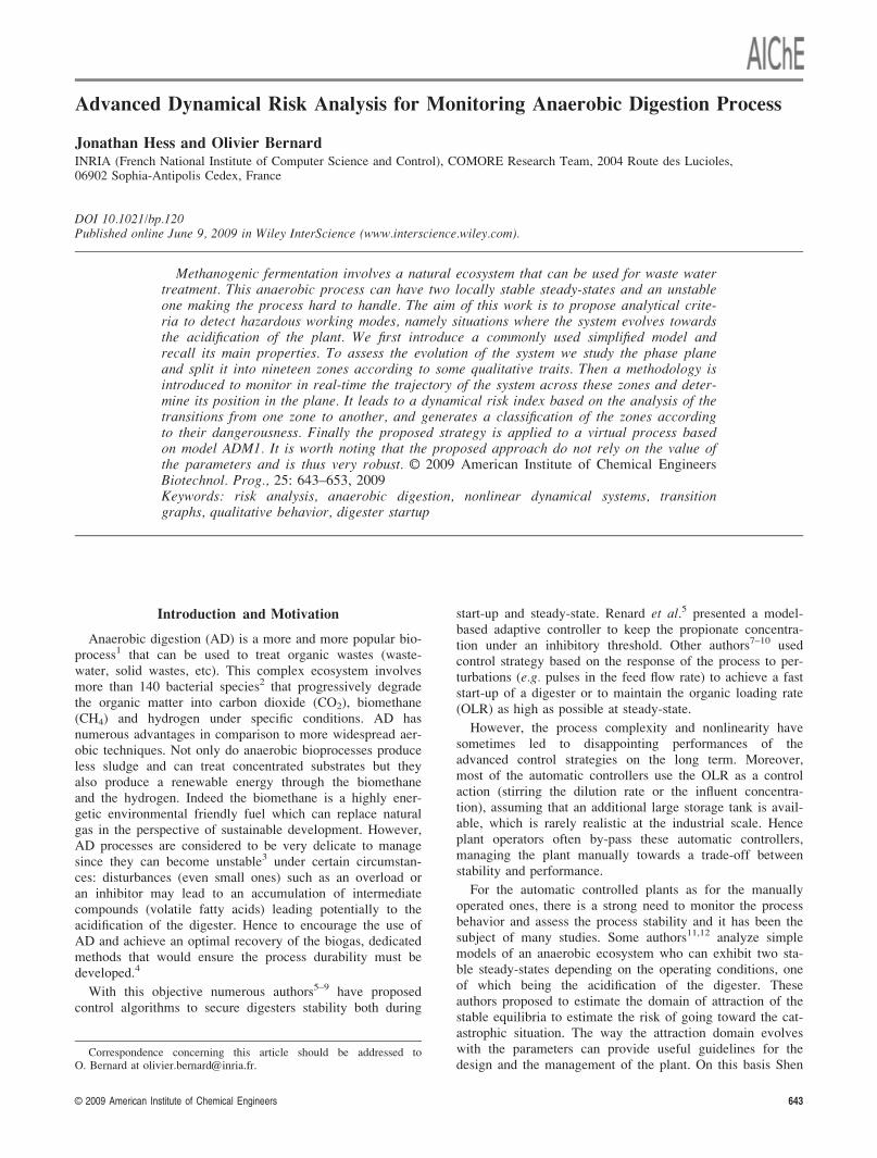
Attraction Basin and Risk Index. Assuming constantoperating conditions, the system behavior strongly dependson the initial conditions as illustrated on Figure 1. Indeed,for some conditions the trajectories will converge towardsn1?2 whereas for other they will reach n

†

2. To evaluate the sys-tem global stability we characterize the set of initials condi-tions leading eventually to n1?2 .

Definition: We define the basin of attraction of theworking point as the set of initial conditions in K for whichthe process converges asymptotically towards the workingpoint n1?2 . More formally, it is defined as:

K1? ¼ n2;0 2 K j limt!þ1 n2ðn2;0; tÞ ¼ n1�2

� �;

we define in the same way the basin of attraction K† for n†

2,as the set of initial conditions leading to the process acidifi-cation:

K† ¼ n2;0 2 K j limt!þ1 n2ðn2;0; tÞ ¼ n†2

� �

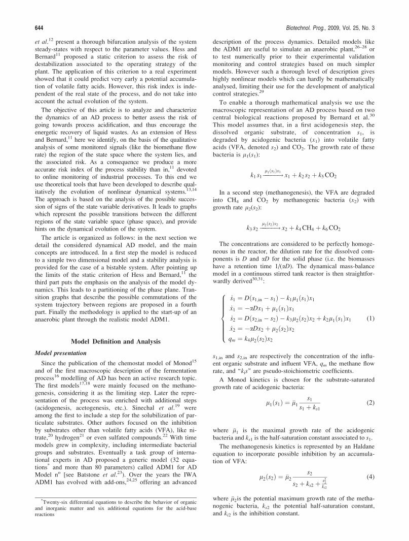
Definition: The separatrix (see Figures 1 and 2) is definedas the curve dividing the plane into the two attraction basins(it is indeed the stable manifold associated to the unstablesteady-state n2?2 ).

Remark: The separatrix can be computed numerically byintegrating system (5) in inverse time starting close to theunstable equilibrium along its stable direction.

It is worth remarking that the bigger the attraction basinK1? the fewer chances that after perturbations the new initialconditions lie in K†, and that eventually the system evolvestowards the acidification. This led Hess and Bernard11 topropose a Stability Index ðISÞ based on the relative size of

Figure 1. Possible trajectories in the phase plane: case whentwo steady-states are stable.

†The total concentration of VFA available for the methanogenesis isequal to the influent VFA s2,in plus the ones produced by the acidogenicbacteria k2

D l1ðs1Þ, and it can be shown that s2;in þ k2D l1

ðs1Þ � s2;in þ k2k1s1;in ¼ ~s2;in.

Biotechnol. Prog., 2009, Vol. 25, No. 3 645

the attraction basin of the working point:

IS ¼ SðK1?ÞSðKÞ

where S is the area of the considered domain.

Ideally the plant manager should choose operating condi-tions that maximize K1? to limit the risk of destabilization.Yet in practice the operator has to simultaneously process amaximal loading and prevent a plant failure.

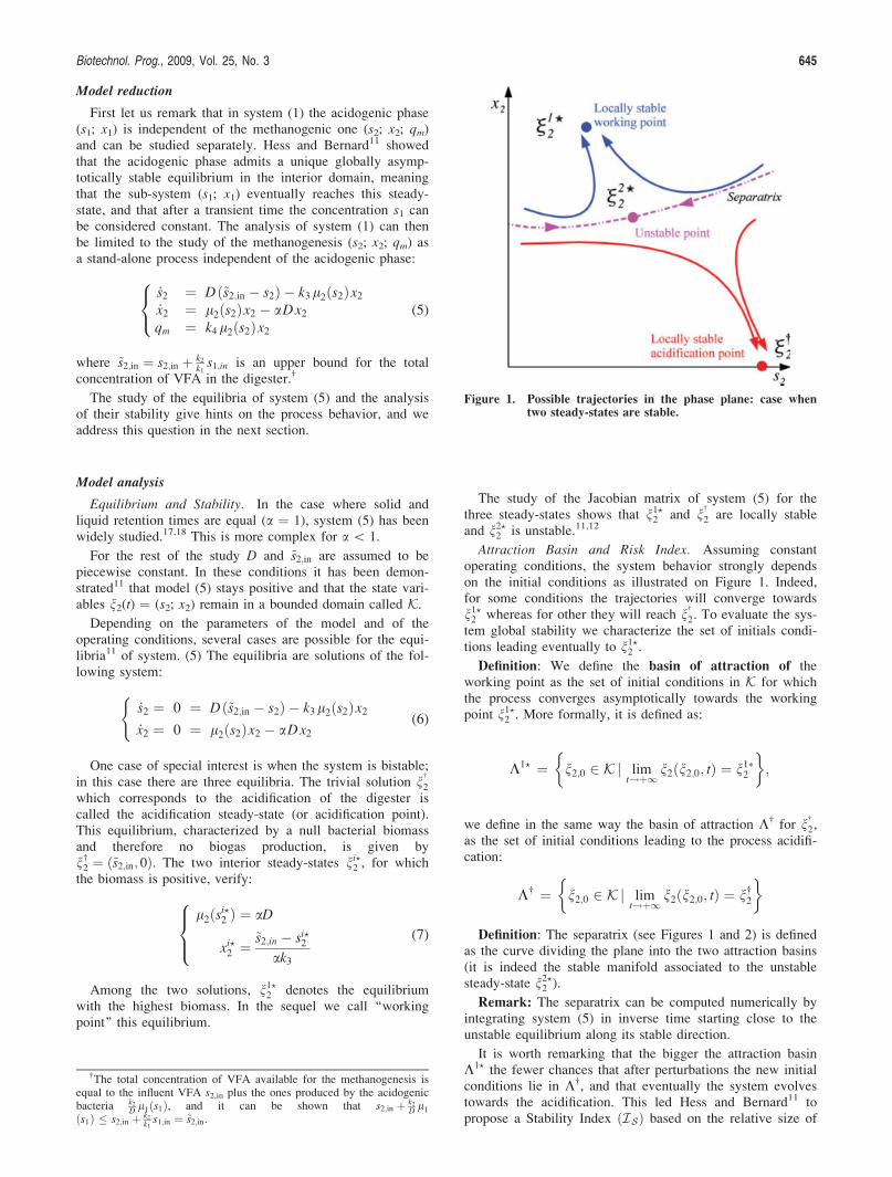
The weakness of this index of stability IS is that it doesnot depend on the real state of the process. As shown onFigure 3 the operating conditions may guarantee a large

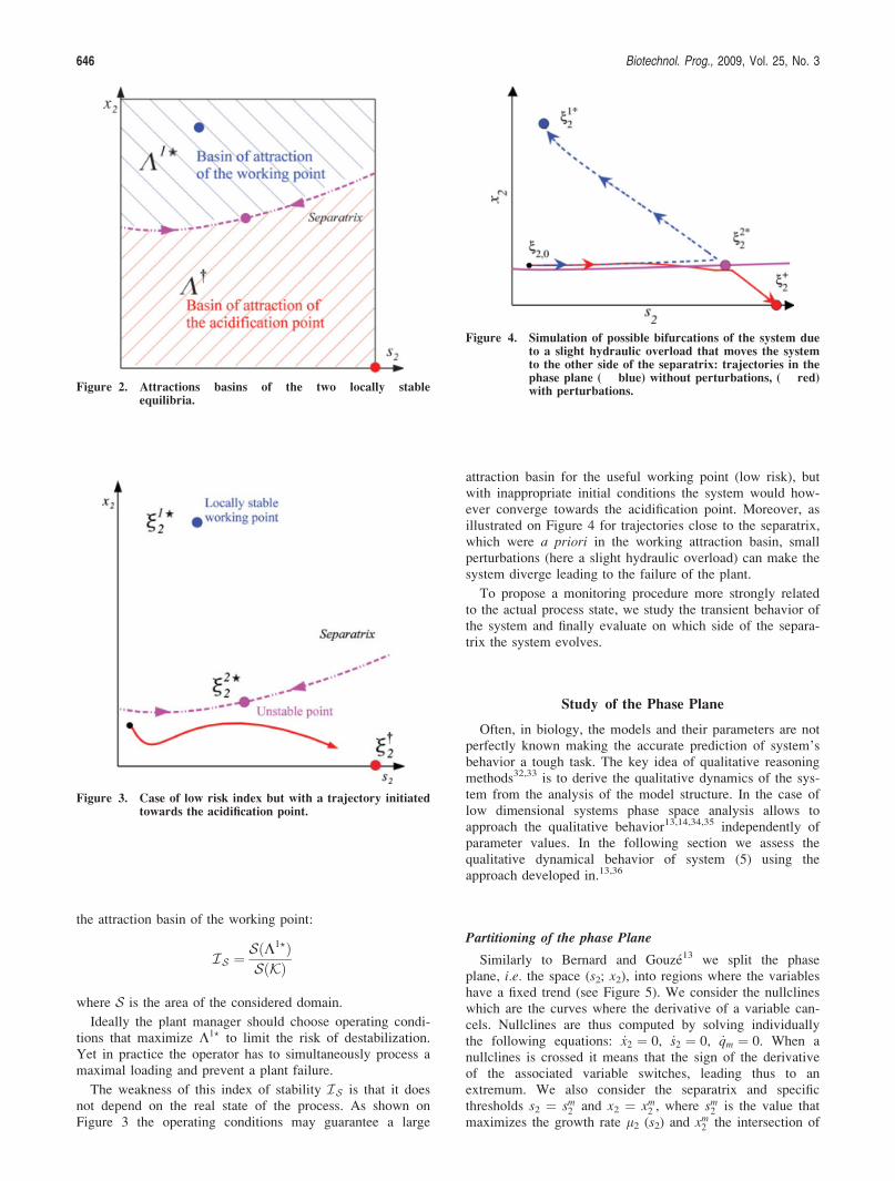
attraction basin for the useful working point (low risk), butwith inappropriate initial conditions the system would how-ever converge towards the acidification point. Moreover, asillustrated on Figure 4 for trajectories close to the separatrix,which were a priori in the working attraction basin, smallperturbations (here a slight hydraulic overload) can make thesystem diverge leading to the failure of the plant.

To propose a monitoring procedure more strongly relatedto the actual process state, we study the transient behavior ofthe system and finally evaluate on which side of the separa-trix the system evolves.

Study of the Phase Plane

Often, in biology, the models and their parameters are notperfectly known making the accurate prediction of system’sbehavior a tough task. The key idea of qualitative reasoningmethods32,33 is to derive the qualitative dynamics of the sys-tem from the analysis of the model structure. In the case oflow dimensional systems phase space analysis allows toapproach the qualitative behavior13,14,34,35 independently ofparameter values. In the following section we assess thequalitative dynamical behavior of system (5) using theapproach developed in.13,36

Partitioning of the phase Plane

Similarly to Bernard and Gouze13 we split the phaseplane, i.e. the space (s2; x2), into regions where the variableshave a fixed trend (see Figure 5). We consider the nullclineswhich are the curves where the derivative of a variable can-cels. Nullclines are thus computed by solving individuallythe following equations: _x2 ¼ 0, _s2 ¼ 0, _qm ¼ 0. When anullclines is crossed it means that the sign of the derivativeof the associated variable switches, leading thus to anextremum. We also consider the separatrix and specificthresholds s2 ¼ sm2 and x2 ¼ xm2 , where sm2 is the value thatmaximizes the growth rate l2 (s2) and xm2 the intersection of

Figure 3. Case of low risk index but with a trajectory initiatedtowards the acidification point.

Figure 4. Simulation of possible bifurcations of the system dueto a slight hydraulic overload that moves the systemto the other side of the separatrix: trajectories in thephase plane ( blue) without perturbations, ( red)with perturbations.Figure 2. Attractions basins of the two locally stable

equilibria.


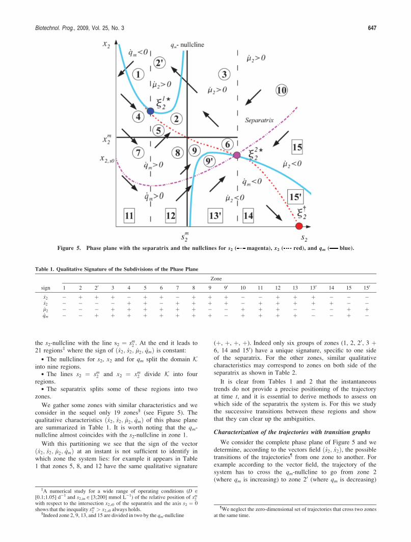
the s2-nullcline with the line s2 ¼ sm2 . At the end it leads to21 regions‡ where the sign of ð _x2; _s2; _l2; _qmÞ is constant:

• The nullclines for s2, x2 and for qm split the domain Kinto nine regions.

• The lines s2 ¼ sm2 and x2 ¼ xm2 divide K into fourregions.

• The separatrix splits some of these regions into twozones.

We gather some zones with similar characteristics and weconsider in the sequel only 19 zones§ (see Figure 5). Thequalitative characteristics ð _x2; _s2; _l2; _qmÞ of this phase planeare summarized in Table 1. It is worth noting that the qm-nullcline almost coincides with the s2-nullcline in zone 1.

With this partitioning we see that the sign of the vectorð _x2; _s2; _l2; _qmÞ at an instant is not sufficient to identify inwhich zone the system lies: for example it appears in Table1 that zones 5, 8, and 12 have the same qualitative signature

(þ, þ, þ, þ). Indeed only six groups of zones (1, 2, 20, 3 þ6, 14 and 150) have a unique signature, specific to one sideof the separatrix. For the other zones, similar qualitativecharacteristics may correspond to zones on both side of theseparatrix as shown in Table 2.

It is clear from Tables 1 and 2 that the instantaneoustrends do not provide a precise positioning of the trajectoryat time t, and it is essential to derive methods to assess onwhich side of the separatrix the system is. For this we studythe successive transitions between these regions and showthat they can clear up the ambiguities.

Characterization of the trajectories with transition graphs

We consider the complete phase plane of Figure 5 and wedetermine, according to the vectors field ð _s2; _x2Þ, the possibletransitions of the trajectories¶ from one zone to another. Forexample according to the vector field, the trajectory of thesystem has to cross the qm-nullcline to go from zone 2(where qm is increasing) to zone 20 (where qm is decreasing)

Figure 5. Phase plane with the separatrix and the nullclines for s2 ( magenta), x2 ( red), and qm ( blue).

Table 1. Qualitative Signature of the Subdivisions of the Phase Plane

sign

Zone

1 2 20 3 4 5 6 7 8 9 90 10 11 12 13 130 14 15 150

_x2 � þ þ þ � þ þ � þ þ þ � � þ þ þ � � �_s2 � � � � þ þ � þ þ þ þ � þ þ þ þ þ � �_l2 � � � þ þ þ þ þ þ � � þ þ þ � � � þ þ_qm � � þ þ þ þ þ þ þ þ � þ þ þ þ � � þ �

‡A numerical study for a wide range of operating conditions (D [[0.1;1.05] d�1 and s2,in [ [3;200] mmol L�1) of the relative position of xm2with respect to the intersection x2;s0 of the separatrix and the axis s2 ¼ 0shows that the inequality xm2 > x2;s0 always holds.

§Indeed zone 2, 9, 13, and 15 are divided in two by the qm-nullcline

¶We neglect the zero-dimensional set of trajectories that cross two zonesat the same time.


(see Table 1). Thus this transition corresponds to a maxi-mum of the biogas flow-rate.

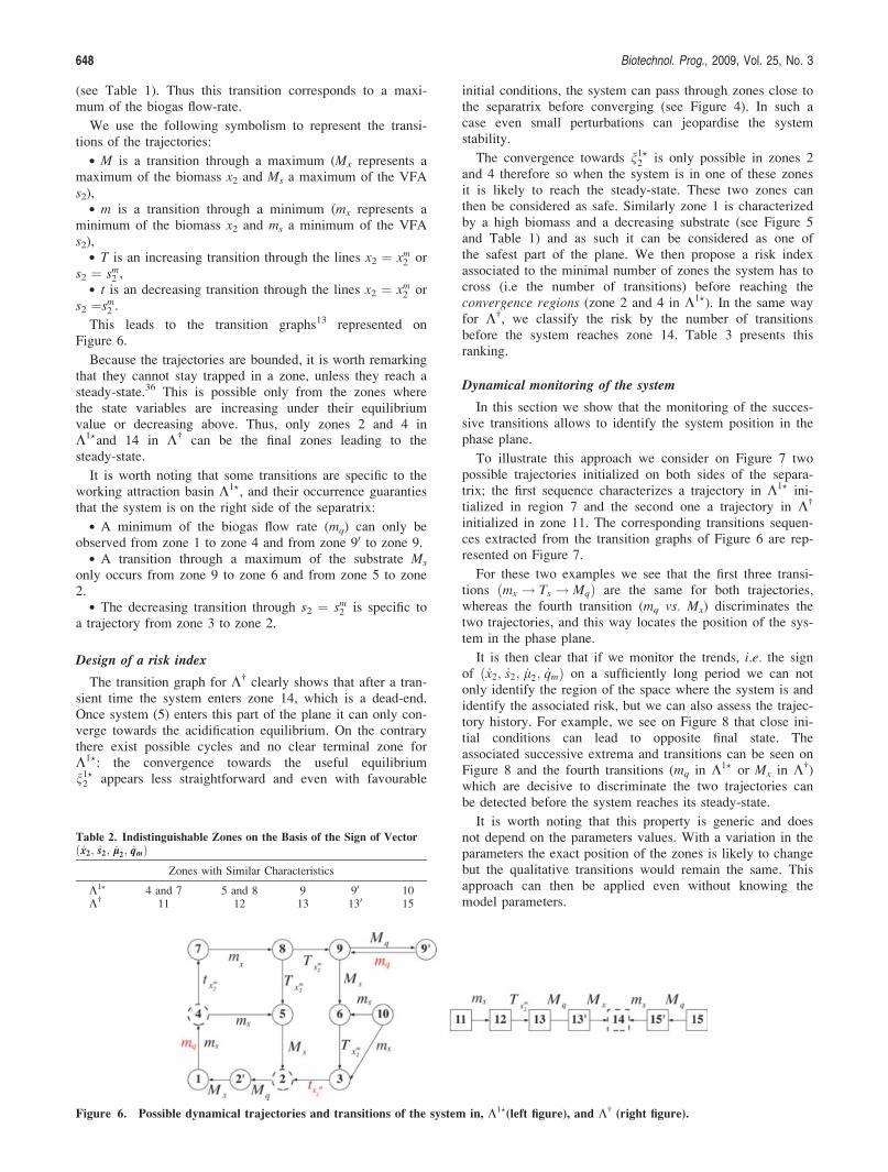
We use the following symbolism to represent the transi-tions of the trajectories:

• M is a transition through a maximum (Mx represents amaximum of the biomass x2 and Ms a maximum of the VFAs2),

• m is a transition through a minimum (mx represents aminimum of the biomass x2 and ms a minimum of the VFAs2),

• T is an increasing transition through the lines x2 ¼ xm2 ors2 ¼ sm2 ,

• t is an decreasing transition through the lines x2 ¼ xm2 ors2 ¼sm2 .

This leads to the transition graphs13 represented onFigure 6.

Because the trajectories are bounded, it is worth remarkingthat they cannot stay trapped in a zone, unless they reach asteady-state.36 This is possible only from the zones wherethe state variables are increasing under their equilibriumvalue or decreasing above. Thus, only zones 2 and 4 inK1?and 14 in K† can be the final zones leading to thesteady-state.

It is worth noting that some transitions are specific to theworking attraction basin K1?, and their occurrence guarantiesthat the system is on the right side of the separatrix:

• A minimum of the biogas flow rate (mq) can only beobserved from zone 1 to zone 4 and from zone 90 to zone 9.

• A transition through a maximum of the substrate Ms

only occurs from zone 9 to zone 6 and from zone 5 to zone2.

• The decreasing transition through s2 ¼ sm2 is specific toa trajectory from zone 3 to zone 2.

Design of a risk index

The transition graph for K† clearly shows that after a tran-sient time the system enters zone 14, which is a dead-end.Once system (5) enters this part of the plane it can only con-verge towards the acidification equilibrium. On the contrarythere exist possible cycles and no clear terminal zone forK1?: the convergence towards the useful equilibriumn1?2 appears less straightforward and even with favourable

initial conditions, the system can pass through zones close tothe separatrix before converging (see Figure 4). In such acase even small perturbations can jeopardise the systemstability.

The convergence towards n1?2 is only possible in zones 2and 4 therefore so when the system is in one of these zonesit is likely to reach the steady-state. These two zones canthen be considered as safe. Similarly zone 1 is characterizedby a high biomass and a decreasing substrate (see Figure 5and Table 1) and as such it can be considered as one ofthe safest part of the plane. We then propose a risk indexassociated to the minimal number of zones the system has tocross (i.e the number of transitions) before reaching theconvergence regions (zone 2 and 4 in K1?). In the same wayfor K†, we classify the risk by the number of transitionsbefore the system reaches zone 14. Table 3 presents thisranking.

Dynamical monitoring of the system

In this section we show that the monitoring of the succes-sive transitions allows to identify the system position in thephase plane.

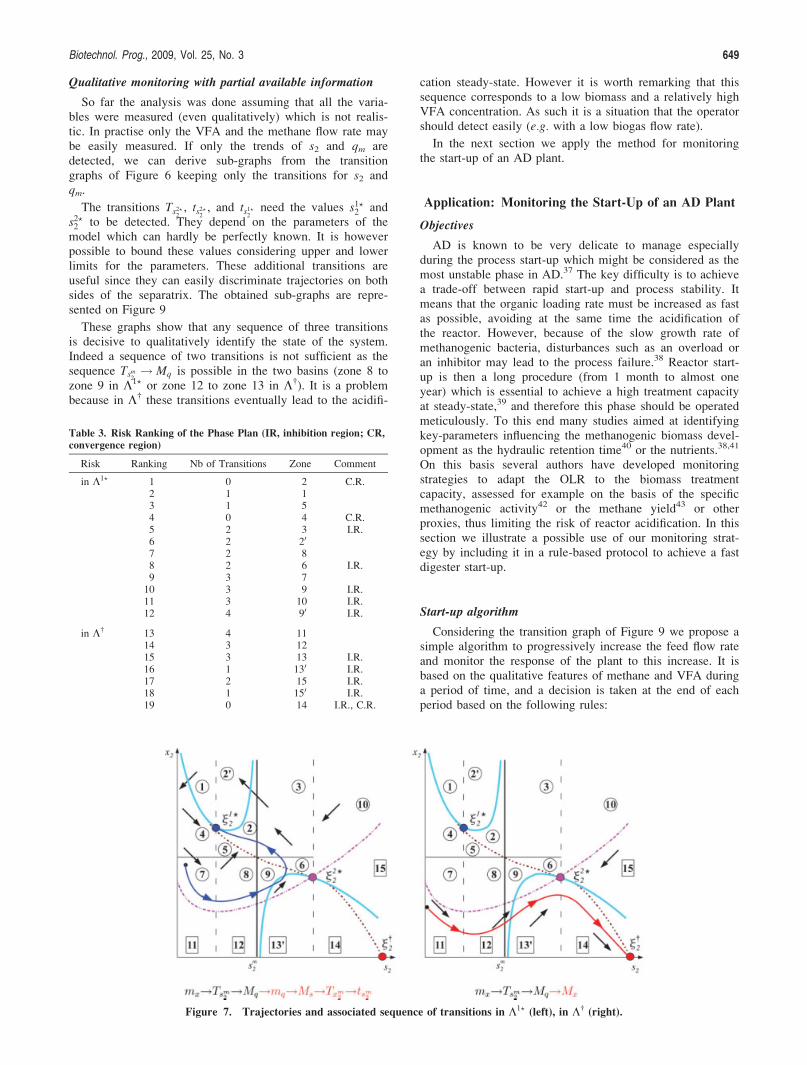
To illustrate this approach we consider on Figure 7 twopossible trajectories initialized on both sides of the separa-trix; the first sequence characterizes a trajectory in K1? ini-tialized in region 7 and the second one a trajectory in K†

initialized in zone 11. The corresponding transitions sequen-ces extracted from the transition graphs of Figure 6 are rep-resented on Figure 7.

For these two examples we see that the first three transi-tions ðmx ! Ts ! MqÞ are the same for both trajectories,whereas the fourth transition (mq vs. Mx) discriminates thetwo trajectories, and this way locates the position of the sys-tem in the phase plane.

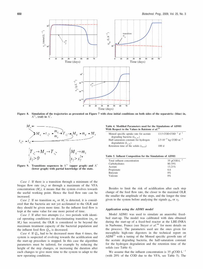
It is then clear that if we monitor the trends, i.e. the signof ð _x2; _s2; _l2; _qmÞ on a sufficiently long period we can notonly identify the region of the space where the system is andidentify the associated risk, but we can also assess the trajec-tory history. For example, we see on Figure 8 that close ini-tial conditions can lead to opposite final state. Theassociated successive extrema and transitions can be seen onFigure 8 and the fourth transitions (mq in K1? or Mx in K†)which are decisive to discriminate the two trajectories canbe detected before the system reaches its steady-state.

It is worth noting that this property is generic and doesnot depend on the parameters values. With a variation in theparameters the exact position of the zones is likely to changebut the qualitative transitions would remain the same. Thisapproach can then be applied even without knowing themodel parameters.

Table 2. Indistinguishable Zones on the Basis of the Sign of Vector

ð _x2; _s2; _l2; _qmÞZones with Similar Characteristics

K1? 4 and 7 5 and 8 9 90 10K† 11 12 13 130 15

Figure 6. Possible dynamical trajectories and transitions of the system in, K1?(left figure), and K†(right figure).


Qualitative monitoring with partial available information

So far the analysis was done assuming that all the varia-bles were measured (even qualitatively) which is not realis-tic. In practise only the VFA and the methane flow rate maybe easily measured. If only the trends of s2 and qm aredetected, we can derive sub-graphs from the transitiongraphs of Figure 6 keeping only the transitions for s2 andqm.

The transitions Ts2?2, ts2?

2, and ts1?

2need the values s1?2 and

s2?2 to be detected. They depend on the parameters of themodel which can hardly be perfectly known. It is howeverpossible to bound these values considering upper and lowerlimits for the parameters. These additional transitions areuseful since they can easily discriminate trajectories on bothsides of the separatrix. The obtained sub-graphs are repre-sented on Figure 9

These graphs show that any sequence of three transitionsis decisive to qualitatively identify the state of the system.Indeed a sequence of two transitions is not sufficient as thesequence Tsm

2! Mq is possible in the two basins (zone 8 to

zone 9 in K1? or zone 12 to zone 13 in K†). It is a problembecause in K† these transitions eventually lead to the acidifi-

cation steady-state. However it is worth remarking that thissequence corresponds to a low biomass and a relatively highVFA concentration. As such it is a situation that the operatorshould detect easily (e.g. with a low biogas flow rate).

In the next section we apply the method for monitoringthe start-up of an AD plant.

Application: Monitoring the Start-Up of an AD Plant

Objectives

AD is known to be very delicate to manage especiallyduring the process start-up which might be considered as themost unstable phase in AD.37 The key difficulty is to achievea trade-off between rapid start-up and process stability. Itmeans that the organic loading rate must be increased as fastas possible, avoiding at the same time the acidification ofthe reactor. However, because of the slow growth rate ofmethanogenic bacteria, disturbances such as an overload oran inhibitor may lead to the process failure.38 Reactor start-up is then a long procedure (from 1 month to almost oneyear) which is essential to achieve a high treatment capacityat steady-state,39 and therefore this phase should be operatedmeticulously. To this end many studies aimed at identifyingkey-parameters influencing the methanogenic biomass devel-opment as the hydraulic retention time40 or the nutrients.38,41

On this basis several authors have developed monitoringstrategies to adapt the OLR to the biomass treatmentcapacity, assessed for example on the basis of the specificmethanogenic activity42 or the methane yield43 or otherproxies, thus limiting the risk of reactor acidification. In thissection we illustrate a possible use of our monitoring strat-egy by including it in a rule-based protocol to achieve a fastdigester start-up.

Start-up algorithm

Considering the transition graph of Figure 9 we propose asimple algorithm to progressively increase the feed flow rateand monitor the response of the plant to this increase. It isbased on the qualitative features of methane and VFA duringa period of time, and a decision is taken at the end of eachperiod based on the following rules:

Table 3. Risk Ranking of the Phase Plan (IR, inhibition region; CR,

convergence region)

Risk Ranking Nb of Transitions Zone Comment

in K1? 1 0 2 C.R.2 1 13 1 54 0 4 C.R.5 2 3 I.R.6 2 207 2 88 2 6 I.R.9 3 710 3 9 I.R.11 3 10 I.R.12 4 90 I.R.

in K† 13 4 1114 3 1215 3 13 I.R.16 1 130 I.R.17 2 15 I.R.18 1 150 I.R.19 0 14 I.R., C.R.

Figure 7. Trajectories and associated sequence of transitions in K1? (left), in K†(right).


Case 1. If there is a transition through a minimum of thebiogas flow rate (mq) or through a maximum of the VFAconcentration (Ms), it means that the system evolves towardsthe useful working point. Hence the feed flow rate can beincreased.Case 2. If no transition mq or Ms is detected, it is consid-

ered that the bacteria are not yet acclimated to the OLR andthey should be given more time. So the influent feed flow iskept at the same value for one more period of time.Case 3. If after two attempts (i.e. two periods with identi-

cal operating conditions) no discriminating transition (mq orMs) has occurred, the OLR is considered to be beyond themaximum treatment capacity of the bacterial population andthe influent feed flow Qin is decreased.Case 4. If Qin had to be decreased more than 4 times, the

system is suspected of evolving towards the acidification andthe start-up procedure is stopped. In this case the algorithmparameters must be tailored, for example by reducing theheight of the step changes, or increasing the duration aftereach changes to give more time to the system to adapt to thenew operating conditions.

Besides to limit the risk of acidification after each stepchange of the feed flow rate, the closer to the maximal OLRthe smaller the amplitude of the steps, and the longer the timegiven to the system before analysing the signals qm or s2.

Application using the ADM1 model

Model ADM1 was used to simulate an anaerobic fixed-bed start-up. The model was calibrated with data obtainedduring the start-up of a fixed-bed reactor at the LBE-INRAin Narbonne, France (see Steyer et al.44 for more details onthe process). The parameters used are the ones given formesophilic high-rate digesters in the technical report onADM23 with a tuning of the Monod specific growth rate ofthe acetate degrading bacteria, the half-saturation constantfor the hydrogen degradation and the retention time of thesolids (see Table 4).

We assume that the influent concentration is 35 gCOD L�1

(with 20% of the COD due to the VFA, see Table 5). The

Figure 8. Simulation of the trajectories as presented on Figure 7 with close initial conditions on both sides of the separatrix: (blue) in,K1?, (red) in K†

.

Table 4. Modified Parameters used for the Simulations of ADM1

With Respect to the Values in Batstone et al.23

Monod specific uptake rate for acetatedegrading bacteria (km_ac)

13.5 COD�COD�1 d�1

Half-saturation constant for hydrogendegradation (ks_h2)

2.5�10�5 kg COD m�3

Retention time of the solids (tres,X) 100 d

Table 5. Influent Composition for the Simulations of ADM1

Total influent concentration 35 gCOD.L�1

Carbohydrates 80.19%Acetate 13.21%Propionate 6.6Butyrate 0%Valerate 0%

Figure 9. Transitions sequences in K1? (upper graph) and K†

(lower graph) with partial knowledge of the state.


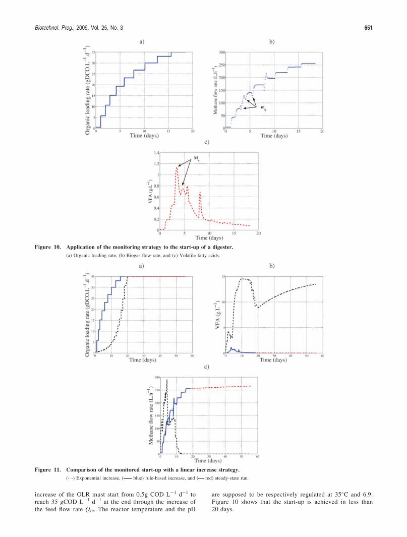
increase of the OLR must start from 0.5g COD L�1 d�1 toreach 35 gCOD L�1 d�1 at the end through the increase ofthe feed flow rate Qin. The reactor temperature and the pH

are supposed to be respectively regulated at 35�C and 6.9.Figure 10 shows that the start-up is achieved in less than20 days.

Figure 11. Comparison of the monitored start-up with a linear increase strategy.

(- -) Exponential increase, ( blue) rule-based increase, and ( red) steady-state run.

Figure 10. Application of the monitoring strategy to the start-up of a digester.

(a) Organic loading rate, (b) Biogas flow-rate, and (c) Volatile fatty acids.


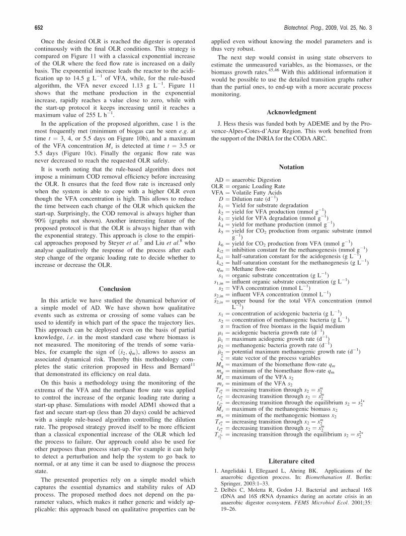
Once the desired OLR is reached the digester is operatedcontinuously with the final OLR conditions. This strategy iscompared on Figure 11 with a classical exponential increaseof the OLR where the feed flow rate is increased on a dailybasis. The exponential increase leads the reactor to the acidi-fication up to 14.5 g L�1 of VFA, while, for the rule-basedalgorithm, the VFA never exceed 1.13 g L�1. Figure 11shows that the methane production in the exponentialincrease, rapidly reaches a value close to zero, while withthe start-up protocol it keeps increasing until it reaches amaximum value of 255 L h�1.

In the application of the proposed algorithm, case 1 is themost frequently met (minimum of biogas can be seen e.g. attime t ¼ 3, 4, or 5.5 days on Figure 10b), and a maximumof the VFA concentration Ms is detected at time t ¼ 3.5 or5.5 days (Figure 10c). Finally the organic flow rate wasnever decreased to reach the requested OLR safely.

It is worth noting that the rule-based algorithm does notimpose a minimum COD removal efficiency before increasingthe OLR. It ensures that the feed flow rate is increased onlywhen the system is able to cope with a higher OLR eventhough the VFA concentration is high. This allows to reducethe time between each change of the OLR which quicken thestart-up. Surprisingly, the COD removal is always higher than90% (graphs not shown). Another interesting feature of theproposed protocol is that the OLR is always higher than withthe exponential strategy. This approach is close to the empiri-cal approaches proposed by Steyer et al.7 and Liu et al.8 whoanalyse qualitatively the response of the process after eachstep change of the organic loading rate to decide whether toincrease or decrease the OLR.

Conclusion

In this article we have studied the dynamical behavior ofa simple model of AD. We have shown how qualitativeevents such as extrema or crossing of some values can beused to identify in which part of the space the trajectory lies.This approach can be deployed even on the basis of partialknowledge, i.e. in the most standard case where biomass isnot measured. The monitoring of the trends of some varia-bles, for example the sign of ð _s2; _qmÞ, allows to assess anassociated dynamical risk. Thereby this methodology com-pletes the static criterion proposed in Hess and Bernard11

that demonstrated its efficiency on real data.

On this basis a methodology using the monitoring of theextrema of the VFA and the methane flow rate was appliedto control the increase of the organic loading rate during astart-up phase. Simulations with model ADM1 showed that afast and secure start-up (less than 20 days) could be achievedwith a simple rule-based algorithm controlling the dilutionrate. The proposed strategy proved itself to be more efficientthan a classical exponential increase of the OLR which ledthe process to failure. Our approach could also be used forother purposes than process start-up. For example it can helpto detect a perturbation and help the system to go back tonormal, or at any time it can be used to diagnose the processstate.

The presented properties rely on a simple model whichcaptures the essential dynamics and stability rules of ADprocess. The proposed method does not depend on the pa-rameter values, which makes it rather generic and widely ap-plicable: this approach based on qualitative properties can be

applied even without knowing the model parameters and isthus very robust.

The next step would consist in using state observers toestimate the unmeasured variables, as the biomasses, or thebiomass growth rates.45,46 With this additional information itwould be possible to use the detailed transition graphs ratherthan the partial ones, to end-up with a more accurate processmonitoring.

Acknowledgment

J. Hess thesis was funded both by ADEME and by the Pro-vence-Alpes-Cotes-d’Azur Region. This work benefited fromthe support of the INRIA for the CODAARC.

Notation

AD ¼ anaerobic DigestionOLR ¼ organic Loading RateVFA ¼ Volatile Fatty Acids

D ¼ Dilution rate (d�1)k1 ¼ Yield for substrate degradationk2 ¼ yield for VFA production (mmol g�1)k3 ¼ yield for VFA degradation (mmol g�1)k4 ¼ yield for methane production (mmol g�1)k5 ¼ yield for CO2 production from organic substrate (mmol

g�1)k6 ¼ yield for CO2 production from VFA (mmol g�1)ki2 ¼ inhibition constant for the methanogenesis (mmol g�1)ks1 ¼ half-saturation constant for the acidogenesis (g L�1)ks2 ¼ half-saturation constant for the methanogenesis (g L�1)qm ¼ Methane flow-rates1 ¼ organic substrate concentration (g L�1)

s1,in ¼ influent organic substrate concentration (g L�1)s2 ¼ VFA concentration (mmol L�1)

s2,in ¼ influent VFA concentration (mmol L�1)~s2;in ¼ upper bound for the total VFA concentration (mmol

L�1)x1 ¼ concentration of acidogenic bacteria (g L�1)x2 ¼ concentration of methanogenic bacteria (g L�1)a ¼ fraction of free biomass in the liquid mediuml1 ¼ acidogenic bacteria growth rate (d�1)�l1 ¼ maximum acidogenic growth rate (d�1)l2 ¼ methanogenic bacteria growth rate (d�1)�l2 ¼ potential maximum methanogenic growth rate (d�1)n ¼ state vector of the process variables

Mq ¼ maximum of the biomethane flow-rate qmmq ¼ minimum of the biomethane flow-rate qmMs ¼ maximum of the VFA s2ms ¼ minimum of the VFA s2Tsm

2¼ increasing transition through s2 ¼ sm2

tsm2¼ decreasing transition through s2 ¼ sm2

tsi?2¼ decreasing transition through the equilibrium s2 ¼ s1?2

Mx ¼ maximum of the methanogenic biomass x2mx ¼ minimum of the methanogenic biomass x2Txm

2¼ increasing transition through x2 ¼ xm2

txm2¼ decreasing transition through x2 ¼ xm2

Ts2?2¼ increasing transition through the equilibrium s2 ¼ s2?2

Literature cited

1. Angelidaki I, Ellegaard L, Ahring BK. Applications of theanaerobic digestion process. In: Biomethanation II. Berlin:Springer, 2003:1–33.

2. Delbes C, Moletta R, Godon J-J. Bacterial and archaeal 16SrDNA and 16S rRNA dynamics during an acetate crisis in ananaerobic digestor ecosystem. FEMS Microbiol Ecol. 2001;35:19–26.


3. Fripiat J, Bol TR, Binot HN, Nyns E. A strategy for the evalu-ation of methane production from different types of substratebiomass. In: Buvet R, Fox M, Picker D, editors, Biomethane,Production and Uses, Exeter, UK: Roger Bowskill, 1984:95–105.

4. Steyer J-P, Aceves C, Ramirez I, Helias A, Hess J, Bernard O,Nielsen HB, Boe K, Angelidaki I. Optimizing biogas produc-tion from anaerobic digestion. In: Proceedings of WEFTEC.06,Dallas, US, 2006.

5. Renard P, Van Breusegem V, Nguyen M-T, Naveau H, Nyns E-J. Implementation of an adaptative conroller for the startup andsteady-state running of a biomethanation process operated in theCSTR. Biotechnol Bioeng. 1991;38:805–812.

6. Pullammanappallil P, Harmon J, Chynoweth DP, Lyberatos G,Svoronos SA. Avoiding digester imbalance through real-timeexpert system control of dilution rate. Appl Biochem Biotechnol.1991;28–29:33–42.

7. Steyer J-P, Buffiere P, Rolland D, Moletta R. Advanced controlof anaerobic digestion processes through disturbances monitor-ing. Water Res. 1999;33:2059–2068.

8. Liu J, Olsson G, Mattiasson B. Monitoring and control of an an-aerobic upflow fixed-bed reactor for high-loading-rate operationand rejection of disturbances. Biotechnol Bioeng. 2004;87:44–55.

9. von Sachs J, Meyer U, Rys P, Feitkenhuer H. New approach tocontrol the methanogenic reactor of a two-phase anaerobicdigestion system. Water Res. 2003;37:973–982.

10. Akesson M, Hagander P, Axelsson J-P. A probing feeding strategyfor Escherichia coli cultures. Biotechnol Tech. 1999;13:523–528.

11. Hess J, Bernard O. Design and study of a risk management cri-terion for an unstable anaerobic wastewater treatment process. JProcess Control. 2008;18:71–79.

12. Shen S, Premier GC, Guwy A, Dinsdale R. Bifurcation and sta-bility analysis of an anaerobic digestion model. NonlinearDynam. 2007;48:391–408.

13. Bernard O, Gouze J-L. Global qualitative behavior of a class ofnonlinear biological systems: application to the qualitative vali-dation of phytoplankton growth models. Artif Intell. 2002;136:29–59.

14. de Jong H. Qualitative simulation and related approaches forthe analysis of dynamic systems. Knowledge Eng Rev. 2004;19:93–132.

15. Monod J. Recherches sur la croissance des cultures bacteri-ennes. Hermann & cie, 1942.

16. Illinois State Water Survey Division. Anaerobic Fermentations.State of Illinois: Illinois State Water Survey Division, 1939.

17. Andrews JF. A mathematical model for the continous culture ofmicroorganisms utilizing inhibitory substrates. Biotechnol Bio-eng. 1968;10:707–723.

18. Graef SP, Andrews JF. Mathematical modeling and control ofanaerobic digestion. AIChE Symp Ser. 1973;70:101–131.

19. Sinechal XJ, Installe MJ, Nyns E-J. Differentiation between ace-tate and higher volatile acids in the modeling of the anaerobicbiomethanation process. Botechnol Lett. 1979;1:309–314.

20. Hill DT, Barth CL. A dynamic model for simulation of animalwaste digestion. J WPCF. 1977;10:2129–2143.

21. Mosey FE. Mathematical modelling of the anaerobic digestionprocess : regulatory mechanisms for the formation of short-chain volatile acids from glucose. Water Sci Technol. 1983;15:209–232.

22. Kalyuzhnyi S, Sklyar V, Kucherenko I, a Russkova J, Degtyar-yova N. Methanogenic biodegradation of aromatic amines.Water Sci Technol. 2000;42:363–370.

23. Batstone DJ, Keller J, Angelidaki I, Kalyuzhnyi SV, Pavlosta-this SG, Rozzi A, Sanders WTM, Siegrist H, Vavilin VA.Anaerobic Digestion Model No. 1 (ADM1) Vol. 13. London:IWA Publishing, 2002.

24. Batstone DJ, Keller J, Steyer J-P. A review of ADM1 exten-sions, applications, and analysis: 2002–2005. Water Sci Technol.2006;54:1–10.

25. Fedorovich V, Lens P, Kalyuzhnyi S. Extension of anaerobicdigestion model no. 1 with processes of sulfate reduction. ApplBiochem Biotechnol. 2007;109:33–45.

26. Batstone DJ, Keller J. Industrial applications of the IWA anaer-obic digestion model no. 1. Water Sci Technol. 2003;47:199–206.

27. Parker WJ. Application of the ADM1 model to advanced anaer-obic digestion. Biores Technol. 2005;96:1832–1842.

28. Rosen C, Vrecko D, Gernaey KV, Pons KV, Jeppsson U. Imple-menting ADM1 for plant-wide benchmark simulations in Mat-lab/Simulink. Water Sci Technol. 2006;54:11–9.

29. Simeonov I, Stoyanov S. Modelling and dynamic compensatorcontrol of the anaerobic digestion of organic wastes. Chem Bio-chem Eng Quaterly. 2003;17:285–292.

30. Bernard O, Hadj-Sadok Z, Dochain D, Genovesi A, Steyer J-P.Dynamical model development and parameter identification foran anaerobic wastewater treatment process. Biotechnol Bioeng2001;75:424–438.

31. Bastin G, Dochain D. On-line Estimation and Adaptive Controlof Bioreactors. Amsterdam: Elsevier, 1990.

32. Kuipers B. Commonsense reasoning about causality: derivingbehavior from structure. Artif Intell 1984;24:169–203.

33. Kuipers B. Qualitative simulation. Artif Intell 1986;29:289–338.34. Lee WW, Kuipers B. A qualitative method to construct phase

portraits. In: Eleventh National Conference on Artificial Intelli-gence, Menlo Park, CA. 1993.

35. Kuipers B. Qualitative Reasoning: Modeling and Simulationwith Incomplete Knowledge. Cambridge, MA: MIT Press, 1994.

36. Bernard O, Gouze J-L. Transient behavior of biological loopmodels, with application to the Droop model. Math Biosci.1995;127:19–43.

37. Show K-Y, Wang Y, Foong SF, Tay J-H. Accelerated start-upand enhanced granulation in upflow anaerobic sludge blanketreactors. Water Res. 2004;38:2293–2304.

38. Punal A, Trevisan M, Rozzi A, Lema J. Influence of C:N ratioon the start-up of up-flow anaerobic filter reactors. Water Res.2000;9:2614–2619.

39. Michaud S, Bernet N, Buffiere P, Roustan M, Moletta R. Meth-ane yield as a monitoring parameter for the strat-up of anaero-bic fixed film reactors. Water Res. 2002;36:1385–1391.

40. Cresson R, Escudie R, Carrere H, Delgenes J-P, Bernet N. Influ-ence of hydrodynamic conditions on the start-up of methanogenicinverse turbulent bed reactors. Water Res. 2007;41:603–612.

41. Cresson R, Carrere H, Delgenes J-P, Bernet N. Biofilm forma-tion during the start-up period of an anaerobic biofilm reactor—Impact of the nutrient complementation. Biochem Eng J.2006;30:55–62.

42. Ince O, Anderson GK, Kasapgil B. Control of organic loadingrate using the specific methanogenic activity test during start-upof an anaerobic digestion system. Water Res. 1995;29:349–355.

43. Michaud S, Bernet N, Buffiere P, Delgenes J-P. Use of themethane yield to indicate the metabolic behaviour of methano-genic biofilms. Process Biochem. 2005;40:2751–2755.

44. Steyer J-P, Bouvier JC, Conte T, Gras P, Sousbie P. Evaluationof a four year experience with a fully instrumented anaerobicdigestion process. Water Sci Technol. 2002;45:495–502.

45. Chachuat B, Bernard O. Probabilistic observers for mass-balance based bioprocess models. Int J Robust Nonlinear Con-trol. 2005;16:157–171.

46. Moisan M, Bernard O, Gouze J-L. Near optimal interval observ-ers bundle for uncertain bioreactors. Automatica. In press.

Manuscript received July 29, 2008, and revision received Aug. 27,2008.


advanced dynamical risk analysis for monitoring anaerobic digestion process

Documents