advanced design and verification … · d2.4 issue: 1 partners / clients: fp7 framework programme...
TRANSCRIPT

ADVANCED DESIGN AND VERIFICATION ENVIRONMENT FOR CYBER-PHYSICAL SYSTEM ENGINEERING www.advance-‐ict .eu
D.2.4 - FULL APPLICATION IN THE SMART ENERGY DOMAIN ADVANCE
Grant Agreement: 287563 Date: 30/11/2014 Pages:
80 Status:
Final Authors:
Brett Bicknell, Karim Kanso CSWT Reference:
D2.4
Issue: 1
Partners / Clients:
FP7 Framework Programme European Union
Consortium Members:
University of Southampton
Critical Software Technologies
Alstom Transport Systerel Heinrich Heine Selex ES
Universität

Project ADVANCE
Grant Agreement 287563 “Advanced Design and Verification Environment for
Cyber-physical System Engineering”
ADVANCE Deliverable D.2.4
Full Application in the Smart Energy Domain
Public Document
December 08th
, 2014
http://www.advance-ict.eu

CRITICAL SOFTWARE TECHNOLOGIES LTD 4 BENHAM ROAD SOUTHAMPTON SCIENCE PARK – CHILWORTH SOUTHAMPTON - SO16 7QJ – UNITED KINGDOM
CRITICAL SOFTWARE, S.A. PARQUE INDUSTRIAL DE TAVEIRO, LOTE 48, 3045-504 COIMBRA PORTUGAL
TEMPLATE: CSWT-2008-TPL-00260 ©2014 CRITICAL SOFTWARE TECHNOLOGIES LTD SOUTHAMPTON
FULL APPLICATION IN THE SMART ENERGY DOMAIN ADVANCE
Approval
Name Function Signature Date
John Colley Project Co-Ordinator 08/12/2014
Luke Walsh Project Manager 08/12/2014
Authors and Contributors
Name Contact Description Date
Brett Bicknell [email protected] Author 31/10/2014
Karim Kanso [email protected] Author 31/10/2014
Neil Rampton [email protected] Contributor 31/10/2014
Daniel McLeod [email protected] Contributor 31/10/2014
José Reis [email protected] Contributor 10/11/2014
Access List
Internal Access
Project Team, Engineering Department
External Access
Public Document
The contents of this document are under copyright of Critical Software Technologies. it is released on condition that it shall not be copied in whole, in part or otherwise reproduced (whether by photographic, or any other method) and the contents therefore shall not be divulged to any person other than that of the addressee (save to other authorized offices of his organization having need to know such contents, for the purpose for which disclosure is made) without prior written consent of submitting company.
Revision History
Issue Date Description Author
0.1 31-10-2014 Initial draft Brett Bicknell,
Karim Kanso
0.2 19-11-2014 Internal review Brett Bicknell,
Karim Kanso
1.0 28-11-2014 Final version Brett Bicknell,
Karim Kanso
1.1 08-12-2014 New version produced as a result of Scientific Karim Kanso,

CRITICAL SOFTWARE TECHNOLOGIES LTD 4 BENHAM ROAD SOUTHAMPTON SCIENCE PARK – CHILWORTH SOUTHAMPTON - SO16 7QJ – UNITED KINGDOM
CRITICAL SOFTWARE, S.A. PARQUE INDUSTRIAL DE TAVEIRO, LOTE 48, 3045-504 COIMBRA PORTUGAL
TEMPLATE: CSWT-2008-TPL-00260 ©2014 CRITICAL SOFTWARE TECHNOLOGIES LTD SOUTHAMPTON
Revision History
Issue Date Description Author
Coordinator Final comments José Reis

ADVANCE FULL APPLICATION IN THE SMART ENERGY DOMAIN
PRINTED ON 08/12/2014 4 / 80 CSWT-EUADV-2014-RPT-00407-1.1
TABLE OF CONTENTS 1. EXECUTIVE SUMMARY .................................................................................................................................... 5
2. INTRODUCTION ................................................................................................................................................... 6
2.1 OBJECTIVE ......................................................................................................................................................... 6 2.2 AUDIENCE .......................................................................................................................................................... 6 2.3 DEFINITIONS AND ACRONYMS ........................................................................................................................... 6 2.4 DOCUMENT STRUCTURE .................................................................................................................................... 7
3. DOCUMENTS ......................................................................................................................................................... 8
3.1 APPLICABLE DOCUMENTS ................................................................................................................................. 8 3.2 REFERENCE DOCUMENTS .................................................................................................................................. 8
4. CASE STUDY OVERVIEW ................................................................................................................................. 9
5. PROGRESS SUMMARY .................................................................................................................................... 12
5.1 OBJECTIVES REVIEW ....................................................................................................................................... 14
6. FINAL REPORT ON PROGRESS (APRIL 2014 – NOVEMBER 2014) ................................................... 15
6.1 MODELLING UPDATES ..................................................................................................................................... 15 6.2 CO-SIMULATION .............................................................................................................................................. 48 6.3 VISUALISATION ................................................................................................................................................ 57
7. CONCLUSIONS ................................................................................................................................................... 60
7.1 OVERALL STRATEGY ADOPTED AND TOOLS UTILISED ................................................................................. 60 7.2 INFLUENCE ON TOOL DEVELOPMENT .............................................................................................................. 62 7.3 SUCCESSES AND BENEFITS .............................................................................................................................. 71 7.4 FAILURES AND DISADVANTAGES .................................................................................................................... 74 7.5 REVIEW OF ADVANCE METHODOLOGY BY SELEX ES ............................................................................... 76 7.6 LESSONS LEARNT ............................................................................................................................................ 78 7.7 RECOMMENDATIONS ....................................................................................................................................... 79

ADVANCE FULL APPLICATION IN THE SMART ENERGY DOMAIN
PRINTED ON 08/12/2014 5 / 80 CSWT-EUADV-2014-RPT-00407-1.1
1. Executive Summary
This document reports the substantial progress made on WP2 and reflects on the
experience of applying the ADVANCE framework to a Smart Grid Subsystem - Low Voltage
Control System. This report details the progress made towards the objectives set for WP2,
that is:
1) Using ADVANCE tools and techniques, model and verify the smart grid case study
and demonstrate the efficacy of ADVANCE over more traditional engineering methods,
more specifically:
a) Assess the usability of the Multi-simulation framework (developed in WP4)
in the modelling and simulation of low voltage networks – This is detailed
in Section 6.2 and conclusions are presented in Section 7.3 and 7.4.
b) Assess the usability of diagrams available in Rodin to represent the
system architecture and behaviour (e.g. component view, iUML-B, state
machines, BMotion Studio). This is detailed in Section 6.3
c) Perform the integration of the method for safety analysis (STPA) in the
verification of the impact of voltage variations on the distribution network.
This is detailed in Section 6.1.1.
d) Assess the suitability of code generation from Event-B models in the
context of this case study. As the work evolved and considerable effort
was placed on the demonstration of the co-simulation framework the
consortium and in particular Selex ES agreed that this was a lower priority,
nevertheless Section 7.4 provides an assessment of this capability.
2) Support the industrial partner in the verification of the solution proposed to manage
voltage on Low Voltage Networks and in this way bring the methods and tools
developed by the consortium to an industrial level. The conclusions are detailed in
Section 7.3, in addition to this, the industrial partner Selex ES provides an independent
view of the overall experience in using the ADVANCE framework in Section 7.5.
The work conducted over the duration of the project gave CSWT the opportunity to focus
the further development of the process and tools, and identify approaches to using the
various elements of the tools efficiently and effectively. During the course of the project
CSWT raised a number of change requests which are described in Section 7.2 together with
its current status and benefits.
The consortium concluded that the ADVANCE framework offers several benefits over more traditional approaches, in particular it:
enables the identification of ambiguities and flaws in the requirements and design prior to deployment
provides a mechanism to visualise complex models in a format that, for instance, demonstrates implication of system changes to the customer in a way that clearly highlights benefits and drawbacks
offers the ability to perform ‘what-if’ analysis
enables managing the complexity of modelling large scale systems
the simulation used helped demonstrate the system robustness in the presence of non-dependable links
The consortium concluded that the ADVANCE framework requires work to improve the
performance of the toolset and to make it easier to adopt at a commercial level, see sections
7.4 and 7.5 for a detailed list of points to improve.
This report also provides recommendations to enable the toolset to mature to a level that
can be used by industry see Section 7.7.

ADVANCE FULL APPLICATION IN THE SMART ENERGY DOMAIN
PRINTED ON 08/12/2014 6 / 80 CSWT-EUADV-2014-RPT-00407-1.1
2. Introduction
2.1 Objective
This document provides a report on the full application of the ADVANCE methods and tools
to the smart grid case study. The document is composed of an overview of the case study,
updates to the case study development since deliverable D.2.3 [AD-3] and conclusions
regarding the applicability and experience of the ADVANCE methods and tools. The case
study is part of Work Package 2 (WP2) of ADVANCE.
2.2 Audience
Those involved or interested in the smart energy case study of the ADVANCE project, and
members of the ADVANCE consortium.
2.3 Definitions and acronyms
Table 1 presents the list of acronyms used throughout the document.
Acronyms Description
AD Applicable Document
ADVANCE Advanced Design and Verification Environment for Cyber-physical system Engineering
API Application Programming Interface
AWS Amazon Web Services
CREST Centre for Renewable Energy Systems Technology
CSWT Critical Software Technologies, Ltd.
DNO Distribution Network Operator
FMI Functional Mock-up Interface
FMU Functional Mock-up Unit
GPRS General Packet Radio Service
HTML Hyper Text Mark-up Language
LV Low Voltage
MV Medium Voltage
OLTC On Load Tap Changer
PV Photo Voltaic
RD Reference Document
SCADA Supervisory Control And Data Acquisition
SIU Sensor Interface Unit
STPA Systems-Theoretic Process Analysis
SVG Scalable Vector Graphics
TRL Technology Readiness Level
UML Unified Modelling Language
UDUS University of Dusseldorf
UOS University of Southampton
WP Work Package
Table 1: Table of acronyms

ADVANCE FULL APPLICATION IN THE SMART ENERGY DOMAIN
PRINTED ON 08/12/2014 7 / 80 CSWT-EUADV-2014-RPT-00407-1.1
2.4 Document structure
Section 1 (Executive Summary) summarises the document.
Section 2 (Introduction) introduces the document.
Section 3 (Documents) presents the list of applicable and reference documents.
Section 4 (Case Study Overview) provides a recap of the WP2 case study.
Section 5 (Progress Summary) summarises both the previous and current progress on the
case study.
Section 6 (Final Report on Progress (April 2014 – November 2014)) provides a detailed
report of the progress made since the previous report.
Section 7 (Conclusions) discusses success, failures, advantages and disadvantages
identified during the case study, as well as future recommendations for the toolset.

ADVANCE FULL APPLICATION IN THE SMART ENERGY DOMAIN
PRINTED ON 08/12/2014 8 / 80 CSWT-EUADV-2014-RPT-00407-1.1
3. Documents
This section presents the applicable and reference documents for this report.
3.1 Applicable documents
Table 2 presents the list of the documents that are applicable to this report. A document is
considered applicable if it complements this document. All its content is directly applied as if
it was stated as an annex of this document.
Applicable document Document number Issue
[AD-1] ADVANCE Deliverable D.2.1: Smart Grid Case Study
Definition, Critical Software Technologies
CSWT-EUADV-2011-SPC-00621 1
[AD-2] ADVANCE Deliverable D.2.2: Proof of Concept
Application in Smart Energy Domain, Critical Software
Technologies
CSWT-EUADV-2012-TNR-00180 1
[AD-3] ADVANCE Deliverable D.2.3: Technical Report on
Assessment of Methods
CSWT-EUADV-2013-RPT-00382 2
Table 2: Applicable documents
3.2 Reference documents
Table 3 lists the reference documents for the report. A document is considered a reference if
it is referred but not applicable to this document. Reference documents are mainly used to
provide further reading.
Reference document Document number Issue
[RD-1] Shared Event Composition/Decomposition in Event-B, University
of Southampton, November 2010
LNCS, 2012, Volume 6957/2012, 122-141
-
[RD-2] Integrated high-resolution modelling of domestic electricity
demand and low voltage electricity distribution networks, PhD
Thesis, Ian Richardson, Loughborough University, UK, 2010
- -
[RD-3] Functional Mock-up Interface for Co-Simulation, Modelisar, 2010 - 1
[RD-4] Voltage characteristics of electricity supplied by public electricity
networks, BSi, 2010
BS EN 50160 2010
[RD-5] Families and Households, Office for National Statistics, 2013
Available: http://www.ons.gov.uk/ons/rel/family-
demography/families-and-households/2013/rft-tables.xls
- -
[RD-6] 2011 Census: QS406EW Household size, local authorities in
England and Wales
Available: http://www.ons.gov.uk/ons/rel/census/2011-
census/key-statistics-and-quick-statistics-for-wards-and-output-
areas-in-england-and-wales/rft-qs406ew.xls
QS406EW 2011
[RD-7] Weekly solar PV installation & capacity based on registration
date, Feed-in Tariff, Office for National Statistics, 2013
- 2 April 2014
[RD-8] Engineering a Safer World, N. Levison, The MIT Press, 2011 - -
[RD-9] Software Bug Contributed to Blackout, Kevin Poulsen,
SecurityFocus, 2004
- -
Table 3: Reference Documents

ADVANCE FULL APPLICATION IN THE SMART ENERGY DOMAIN
PRINTED ON 08/12/2014 9 / 80 CSWT-EUADV-2014-RPT-00407-1.1
4. Case Study Overview
A trend of increasing levels of automation within the smart energy domain has emerged,
and is set to continue. If this automation is not engineered and managed rigorously, there is
substantial risk of catastrophic failure. For example, the infamous north east USA blackout
in 2003 that effected an estimated 55 million people was in part caused by a race condition
in an energy management system [RD-9]. A case study in the smart energy domain has
been selected for this work package as it is a non-typical domain to apply formal
engineering techniques, yet is typical of a cyber-physical system where there is a high
degree of interdependence between the cyber and physical entities.
Using the Rodin toolset to support the development of an industrial class system within the
smart energy domain has provided a number of valuable insights into the methodology and
toolset. Some of these insights have been directly fed back into the development of the
toolset to improve the overall efficiency and usability of Rodin for industrial class solutions.
The case study has been provided by Selex ES, who have been contracted to identify a
solution for automating the control of the voltage on low voltage networks. These are the
networks that distribute electricity to end users.
Currently the voltage on low voltage networks is controlled manually, and foremost is still
reliant on the concept that energy flows in one particular direction. The issues faced by
Selex ES when implementing the automated solution include:
Patterns of usage of the network are continuously evolving and the power flows on the
network at any time of day are becoming less predictable. This means that adjustments
on the low voltage network may have to be done at any time during the day or night.
This is a challenge considering that the manual approach to changing the voltage – i.e.
sending an engineer to the substation to make a physical change – is expensive and
not a practical solution for dynamic control.
Due to the increased use of distributed micro-generation solutions such as photovoltaic
cells or wind turbines, energy flows in different directions within the energy network.
This can also change dynamically depending on environmental factors. Traditional
methods of planning and voltage control are no longer reliable at the low voltage level,
because there are now several aspects that could change the voltage on the network
between the consumer and the higher level transmission and distribution networks.
Despite the lack of a network usage pattern and the bidirectional flow of energy, the
owner of the network needs to keep voltage levels within regulatory extremes. It is also
important to have finer control over the voltage as it can reduce consumption and
system energy losses (technical losses). Distributed generation increases voltages
towards the end of the feeder (and in the case of photovoltaic generation, only during
the day), while increasing demand from heat pumps and electric vehicles decreases
voltage towards the end of the feeders (see Figure 1).

ADVANCE FULL APPLICATION IN THE SMART ENERGY DOMAIN
PRINTED ON 08/12/2014 10 / 80 CSWT-EUADV-2014-RPT-00407-1.1
Figure 1: Exceeding voltage limits
The proposed solution is aimed towards increasing the level of automation in the network.
This is achieved through a control system which hosts an algorithm to determine the
optimum voltage set point for the secondary substation. This optimum voltage set point is
used to control an On Load Tap Change (OLTC) transformer at the secondary substation
(i.e. at the top of the low voltage network). A number of Sensor Interface Units (SIU) are
deployed to monitor the voltage at various points in the network. These are fitted at the Mid
Points (half way) and End Points (at the end) of each of the feeders connected to the
secondary substation. The SIUs provide reports detailing measurements of voltage and
current from their locations along the feeders to the control system. The voltage control
algorithm uses this information to automatically control the tap changer.
An additional issue which needs to be considered during the implementation of the solution
is that there are a limited number of changes that can be made within the lifetime of the tap
changer. Therefore the algorithm must not only regulate the voltage so that the levels on the
network are always within regulatory limits and minimise the amount of power waste, but
also consider the number of tap changes made in order to maximise the lifetime of the tap
changer. A diagram depicting the solution architecture is shown in Figure 2, and a deeper,
technical overview has been previously described in [AD-3].
PV increases voltage during the day
Heat pumps, electric vehicles, etc.
decrease voltage during evening peak

ADVANCE FULL APPLICATION IN THE SMART ENERGY DOMAIN
PRINTED ON 08/12/2014 11 / 80 CSWT-EUADV-2014-RPT-00407-1.1
Figure 2: Selex ES Scenario Architecture
Critical Software is using the framework developed during ADVANCE to support Selex ES
in the early validation of the solution, system architecture and assumptions prior to actual
implementation. This will include an assessment of the architecture and protocols that have
been proposed, and the identification of any counterexamples where the following system
properties are violated:
the controller never issues an unsafe command which lowers the voltage when it is
already too low, and
the controller never issues an unsafe command which raises the voltage when it is
already too high, and
the controller avoids unnecessary tap changes.
This early validation is of utmost importance for Selex ES as it will provide the means to
increase the confidence on the solution before it is fully rolled out on distribution networks
involving actual customers, reducing engineering costs by identifying issues early in the life
cycle. This case study supplements other validation activities undertaken by Selex ES,
which include field trials of the system at two sites. However, Selex ES has a particular
interest in this methodology as they have not used it before, hence this is seen by Selex ES
as an innovative approach for the system engineering of smart grids. The advantage of
there being trial sites is that it provides a mechanism to assess the benefits of the
ADVANCE methodology in comparison to traditional methods.
Transformer TAP Changer
Algorithm SIU SIU
Substation
Low
Volta
ge N
etw
ork
Data Link
3-Phase Power Line
Any number of the houses will have PV cells.
SCADA Router
SIU SIU
SIU SIU

ADVANCE FULL APPLICATION IN THE SMART ENERGY DOMAIN
PRINTED ON 08/12/2014 12 / 80 CSWT-EUADV-2014-RPT-00407-1.1
5. Progress Summary
This section recaps the state of the case study development at the end of the previous
reporting update in issue 2 of deliverable D.2.3 [AD-3], and summarises the work performed
in the final phase of the case study from April to November 2014.
Figure 3 details the overall modelling strategy and the status of the models at the time of the
previous reporting update in April. At this stage, the models filled with solid white were
completed (up to minor modifications), and those with a diagonal line fill were partially
completed.
Figure 3: Model Development Progress March 2014
During the previous phases of work, the main focus was the development of the algorithm
and low voltage network models, where the goal was to get a proof-of-concept co-simulation
running. The proof-of-concept simulation was limited in that:
The communication network model was abstracted, such that there was no
consideration of realistic delay or packet loss, and a simpler network topology –
which was not fully representative of the real network layout – was used.
Only a subset of the behaviour of the SIUs was modelled, omitting the
acknowledgement and retransmission mechanisms. These mechanisms were
omitted at this stage due to there being no packet loss or realistic delay in the
abstraction of the communication network.
The scenarios were half sized, i.e. only 3 feeders were considered in the low
voltage network model instead of the required 6. This tied into the simpler network
topology mentioned in the first point above.

ADVANCE FULL APPLICATION IN THE SMART ENERGY DOMAIN
PRINTED ON 08/12/2014 13 / 80 CSWT-EUADV-2014-RPT-00407-1.1
The co-simulation step size was large, which reduced the granularity of the
simulation, and hence, the required computation resources for the co-simulation.
As detailed in the next section, as the models were expanded to include the omitted detail
and increase the resolution of the co-simulation (i.e. decrease the step size), further issues
with the efficiency of the co-simulation were revealed, which in part required rework to the
structure of the models.
The following points summarise the development on the case study outlined in Section 4 of
[AD-3] during the previous phases of work:
The Algorithm was modelled using the ADVANCE workflow, starting with the
written requirements and design furnished by Selex ES. This involved applying
System-Theoretic Process Analysis (STPA) to understand the problem domain and
develop system level constraints, which were later used to craft the verification
conditions. State machines (from the graphical iUML-B plug-in) were utilised during
development of the algorithm model. As the model was refined, proof activities
were performed, which revealed a number of issues (these are summarised in
Section 7.3).
The abstract SIU models were created directly in Event-B. The modelled behaviour
was limited to sampling the voltage at regular intervals from the Low Voltage
Network model, averaging these values, and periodically forwarding them onto the
algorithm model through the abstract communication network.
Two possible topologies for the Communication Network were identified by
Selex ES and modelled in Event-B; these were a point-to-point network (using
GPRS or similar) and a dynamic mesh network (see previous report [AD-3] for
more detail). As mentioned, these models were limited in scope. Although the
routing protocols – and dynamic reaction thereof to packet loss and changes in the
network – were modelled, the actual packet loss and realistic delays during
operation of the network were not simulated. As mentioned earlier, a simplified
network topology was also used.
The Tap Changer and Low Voltage Network were modelled within Modelica,
which represent the environment of the system. The tap changer model was
completed, whereas the low voltage network was at half size to help investigate the
efficiency of the co-simulation during the initial proof-of-concept stage.
An additional stochastic Communications Outage Probability & Occurrence
model was completed, with the intention to feed into the development of the
communication network model in the last phase of work, by specifying when
communication loss occurs during the co-simulation in a pseudo-random fashion.
Initial Co-simulation was performed using these reduced scale and complexity
models. The co-simulation was performed at a 5 minute resolution, and it was
found that increasing the resolution resulted in severe efficiency issues, which were
reported to the consortium. As described later in the report, development was
performed on the toolset and structure of the models, to rectify these issues as well
as further efficiency problems found when expanding the models. See Figure 35 for
further information about how the co-simulation was set up during this phase of the
work.
Model Visualisation was investigated. This entailed the creation of a prototype
BMotion Studio (version 1) visualisation for the mesh network that graphically
depicted whether a given node was enabled and the volume of data flowing
between any two given nodes. This visualisation is depicted in Figure 47.

ADVANCE FULL APPLICATION IN THE SMART ENERGY DOMAIN
PRINTED ON 08/12/2014 14 / 80 CSWT-EUADV-2014-RPT-00407-1.1
During the final phase of the project, all the models have been completed, and the co-
simulation and visualisation have been expanded and improved. This has involved:
Expanding the communication network models to encompass the missing
detail in the previous abstraction.
Updating the SIU models to encompass the more sophisticated communication
mechanism built into the units. In parallel with modelling the packet loss and
realistic delay in the communication network model, the retransmission and
acknowledgement mechanisms within the units were included as a series of
refinements.
Scaling the low voltage network to a representative model. This has involved
increasing the number of feeders and tuning the other parameters to be realistic, as
well as factoring in an increased number of SIUs to represent the real network
topology.
Model Validation was performed using the improved multi-simulation framework
and an improved visualisation. The co-simulation utilised scaled up models and an
increased time resolution. The visualisation was redesigned, and moved to the new
version of the BMotion Studio tool. The new visualisation included a display of the
voltage levels at different feeder points as well as a representation of the traffic over
the communication network.
These developments are described in detail in Section 6.
5.1 Objectives Review
The objectives defined in Section 6.3.1 of deliverable D.2.3 [AD-3] for this phase of work are
repeated below with a summary of their progress in italics:
Objective 1. Evaluate use of automated ADVANCE model testing and test coverage
metrics as a way of ensuring validity of the test set used to test the implementation
of the algorithm.
>> STPA was used to identify areas that should be tested, but due to the effort
invested into the multi-simulation and getting it to run efficiently there was not
enough effort left to adequately explore the automated model testing and
coverage methods.
Objective 2. Provide input to Selex ES on the validity of the test set for the tap
changer algorithm.
>> As the test set was not defined as discussed in Objective 1, this was not
achieved. However, the results and the produced animations of the co-
simulation were reported to Selex ES, which aided in the validation of the tap
changer algorithm.
Objective 3. Reflect on framework applicability from an industry perspective and
business benefits.
>> Achieved, see conclusions in Section 7.
Objective 4. Demonstrate ADVANCE multi-simulation of Smart Grid Solutions at the
ADVANCE Industry Days.
>> Achieved, demonstrated at both UOS and UDUS industry days.

ADVANCE FULL APPLICATION IN THE SMART ENERGY DOMAIN
PRINTED ON 08/12/2014 15 / 80 CSWT-EUADV-2014-RPT-00407-1.1
6. Final Report on Progress (April 2014 – November 2014)
This section reports on the final modelling updates, results obtained, and interactions with
the consortium, during the period of April 2014 to the end of the work package.
At the end of the previous reporting update in [AD-3] the first co-simulations had been
evaluated successfully up to 500 time steps (out of a desired 1440). As described in the
previous section, the models at this stage were simplified to test the framework, and only
considered 3 feeders with idealised communications channels. During April 2014 to
November 2014, much of the focus has been on extending the models to a representative
system – with 6 feeders and a more representative communications network – that is also
feasible to use for co-simulation. This entailed numerous experiments to understand the
best modelling approach, in order to take full advantage of the underlying tools and mitigate
scalability issues. The related issue of producing meaningful visualisations of the simulations
was also explored in more depth.
This section is structured into the following subsections:
6.1 Modelling Updates: Provides technical details regarding the changes required to
the models, and any new development.
6.2 Co-Simulation: Details the experiments undertaken to tune the models and
simulation framework, and overviews the continuous models.
6.3 Visualisation: Describes the updates made to the visualisations, and the migration
to the new version of BMotion Studio.
6.1 Modelling Updates
6.1.1 STPA
The previous deliverable provided a rough overview of the STPA process that was
undertaken during this case study. In this subsection, a full application of STPA has been
detailed as defined in Chapter 8 of [RD-8]. This covers the initial phase of determining the
control loop, and the two proceeding phases where the hazards and system constraints are
first identified, and then each hazard’s causes are identified. The mitigation activities were
constrained due to the limitation of the case study architecture being fixed outside of this
case study.
The ADVANCE workflow advocates that the constraints developed during the first phase of
STPA – that prevent or mitigate the hazard – are used to guide the development of Event-B
invariants, and that the causes of the hazards identify system level test cases. Due to time
constraints the causes were not translated into test cases.
6.1.1.1 Control Loop
The initial step of STPA is to develop a control loop diagram that details the control actions
and information flow around the system; see Figure 4. This control loop will serve as the
foundational tool for analysing the system for hazardous behaviour and later, causes of
these hazards.

ADVANCE FULL APPLICATION IN THE SMART ENERGY DOMAIN
PRINTED ON 08/12/2014 16 / 80 CSWT-EUADV-2014-RPT-00407-1.1
Figure 4: Control Loop
The blocks in Figure 4 relate to entities within the system that effect the control loop. These
include the control system, actuators, sensors and the controlled process. The blocks that
emit control actions have internal state, which in following STPA terminology is known as a
process model. The process models are essentially an abstracted view of the controller’s
state that details the essential information which the controllers require to adequately control
the underlying process.
STPA was essential to efficiently identify the system architecture, which was used as the starting point for subsequent modelling.
From Figure 4 it is clear that two control loops exist in the modelled system. The first loop is
controlled by the tap changer and the second loop is controlled by the algorithm. In our case
study we are primarily interested in the second control loop, as the tap changer is
considered part of the environment. However, it is important to consider the system as a
whole at this level.

ADVANCE FULL APPLICATION IN THE SMART ENERGY DOMAIN
PRINTED ON 08/12/2014 17 / 80 CSWT-EUADV-2014-RPT-00407-1.1
6.1.1.2 Safety
Before it is possible to analyse the control loop to identify possible hazards that the algorithm
could cause, a notion of safety is required. This is the underlying safety property that the
system will be developed against. The following safety property is used:
The voltage of the power provided to all customer premises remains within the regulated upper and lower bounds.
Due to underlying designs of the system architecture outside the scope of this case study
the above property will not always hold – as will be discussed in the following sections –
nonetheless it is the underlying goal. Moreover, as this case study concerns delivering
power to dwellings it is not considered safety critical, and there are safety related devices
outside the scope of this analysis that will prevent the system as a whole providing a
dangerous amount of power to the consumers, i.e., power can always be shed to maintain
safety of the occupants.
6.1.1.3 STPA Step 1: Hazards and Constraints
Step 1 of STPA is concerned with analysing each of the possible control actions that a given
control system can emit, and deciding whether they could potentially lead to the safety
property being violated. Then, for each hazard, system level constraints are identified that
prevent these hazards from occurring.
The following subsections detail the hazards and their associated constraints.
6.1.1.3.1 Hazard Identification
The table in Figure 5 identifies the hazards that the algorithm could cause, and the table
structure is archetypal of the STPA process. The increase and decrease control actions are
generalisations of the digital voltage target control action from Figure 4. That is, an increase
voltage control action represents the set target being higher than the previous target (and
symmetrically for the decrease target). When the target does not change, this is equivalent
to no control action being emitted, and is covered by the first row of the table.
INCREASE VOLTAGE DECREASE VOLTAGE
NOT PROVIDING
CAUSES HAZARD
(A) Voltage could fall below legal limit
on LV network.
(D) Voltage could rise above legal
limit on LV network.
PROVIDING CAUSES
HAZARD
(B) Voltage could rise above legal
limit on LV network.
(E) Voltage could fall below legal
limit on LV network.
WRONG
TIMING/ORDER
CAUSES HAZARD
(C) Late: Voltage could fall (or fail to
be raised) above legal limit on LV
network.
(F) Late: Voltage could rise (or fail
to be lowered) below legal limit on
LV network.
STOPPED TOO SOON
OR APPLIED TOO
LONG
Not hazardous Not hazardous
Figure 5: Control Algorithm Hazards

ADVANCE FULL APPLICATION IN THE SMART ENERGY DOMAIN
PRINTED ON 08/12/2014 18 / 80 CSWT-EUADV-2014-RPT-00407-1.1
Hazards A, B and C are symmetric to hazards D, E and F, therefore, in the following only
hazards A, B and C are considered in any depth. It is left to the reader’s intuition to infer the
details for hazards D, E and F.
Figures 6, 7 and 8 depict possible situations under which the hazards A, B and C arise.
Figure 6 describes a situation where, through inaction, the control system lets the
voltage fall below the lower legal limit.
Figure 7 describes a situation where, through over action, the control system drives
the voltage up above the legal limit.
Figure 8 describes a situation where the control system is not responsive enough to
control the voltage. That is, it takes too long to issue the increase voltage control
action so the voltage still falls below the lower limit on the network. The dotted lines
indicate the time periods from when the condition for a tap change is required, to
when it actually occurs, i.e., the delay.
Figure 6: Hazard A
Figure 7: Hazard B

ADVANCE FULL APPLICATION IN THE SMART ENERGY DOMAIN
PRINTED ON 08/12/2014 19 / 80 CSWT-EUADV-2014-RPT-00407-1.1
Figure 8: Hazard C
6.1.1.3.2 Constraints
To prevent the hazards enumerated in Figure 5 from occurring, each hazard is associated
with system level constraints that, if fulfilled, prevent the hazard from occurring.
6.1.1.3.2.1 Hazard A
Not providing causes the hazard: Voltage could fall below legal limit on LV network.
A.1. When voltage falls below the lower threshold at any measured point, the increase
voltage control action is issued.
A.2. When the increase voltage control action is issued, the result will not put the voltage
below the lower limit at any point on the LV network.
6.1.1.3.2.2 Hazard B
Providing causes the hazard: Voltage could rise above legal limit on LV network.
B.1. When the voltage at any measured point is above the upper threshold, the voltage
increase control action must not be issued.
6.1.1.3.2.3 Hazard C
Providing too late causes the hazard: Voltage could fall (or fail to be raised) above
legal limit on LV network.
C.1. The voltage increase command must be issued within x seconds of the measured
voltage at any point being below the lower threshold.
NB. Constraints of hazards D, E and F are symmetric to A, B and C, respectively.
6.1.1.3.2.4 Hazard D
Not providing causes the hazard: Voltage could rise above legal limit on LV network.
D.1. When the voltage rises above the upper threshold at any measured point, the decrease
voltage control action is issued.
D.2. When the decrease voltage control action is issued, the result will not put the voltage
above the upper limit at any point on the LV network.

ADVANCE FULL APPLICATION IN THE SMART ENERGY DOMAIN
PRINTED ON 08/12/2014 20 / 80 CSWT-EUADV-2014-RPT-00407-1.1
6.1.1.3.2.5 Hazard E
Providing causes the hazard: Voltage could fall below legal limit on LV network.
E.1. When the voltage at any measured point is below the lower threshold, the voltage
decrease control action must not be issued.
6.1.1.3.2.6 Hazard F
Providing too late causes the hazard: Voltage could rise (or fail to be lowered) below
legal limit on LV network.
F.1. The voltage decrease command must be issued within x seconds of the measured
voltage at any point being above the upper threshold.
6.1.1.3.2.7 Event-B Invariants
During this case study, instead of directly using the 8 constraints identified above, two
abstract constraints were produced as Event-B invariants, as this proved simpler to model
and rigorously analyse. Using the Rodin toolset, the Event-B models were checked as to
whether they upheld these invariants. This means that, if the proof system found a violation
of either of these invariants, then an undesirable behaviour was identified.
These invariants represent the following two statements:
1. If the voltage is above the defined maximum at any of the measured points, the
target voltage should be decreased at the transformer.
2. If the voltage is below the defined minimum at any of the measured points, the
target voltage should be increased at the transformer.
6.1.1.4 STPA Step 2: Causal Scenarios
The second step of STPA concerns understanding how the constraints identified in the
previous step could be violated, and is the first step for identifying test cases. To represent
this information, the well-known fault tree diagrams have been adopted. These were chosen
as there is an inherent hierarchical nature of events that propagate through the system
which can result in the constraints being violated. Although not undertaken in this project,
the use of fault trees also provides a mechanism to perform further probabilistic risk
assessment.
Due to the system architecture and control loop in Figure 4, the majority of the causes are
based around the process model becoming inconsistent. That is, either an SIU reporting an
invalid measurement, issues with the communications network, or software issues within the
algorithm’s control unit that store the values incorrectly. As such, the following sub-fault tree
encapsulates the reasons that a given variable x could become inconsistent, and is reused
in subsequent trees:

ADVANCE FULL APPLICATION IN THE SMART ENERGY DOMAIN
PRINTED ON 08/12/2014 21 / 80 CSWT-EUADV-2014-RPT-00407-1.1
Figure 9: Fault Tree, Inconsistent Variable
Figure 10: Fault Tree, Constraint A.1

ADVANCE FULL APPLICATION IN THE SMART ENERGY DOMAIN
PRINTED ON 08/12/2014 22 / 80 CSWT-EUADV-2014-RPT-00407-1.1
Figure 11: Fault Tree, Constraint A.2
Figure 12: Fault Tree, Constraint B.1

ADVANCE FULL APPLICATION IN THE SMART ENERGY DOMAIN
PRINTED ON 08/12/2014 23 / 80 CSWT-EUADV-2014-RPT-00407-1.1
Figure 13: Fault Tree, Constraint C.1

ADVANCE FULL APPLICATION IN THE SMART ENERGY DOMAIN
PRINTED ON 08/12/2014 24 / 80 CSWT-EUADV-2014-RPT-00407-1.1
6.1.2 Formal Modelling Strategy
This section details the modelling strategies employed when developing the formal models.
During the co-simulation activities, several refinement and modelling strategies were
investigated before finding the most suitable approach; the successes and drawbacks of
each is discussed. As demonstrated throughout the section, it was found that the refinement
strategy is linked closely to the topology of the simulation, which plays an important role in
determining the most suitable structure of the models.
6.1.2.1 Refinement and Decomposition Overview
Both refinement and decomposition played a key role in managing the complexity and
verification of the formal (Event-B) models. Refinement is the process of introducing details
into abstract Event-B model to create a more concrete model. The refined model can
introduce additional properties or behaviour to the model, or it can extend abstract
behaviour already in place. Decomposition, on the other hand, provides the means to
separate out the contents of an Event-B model into multiple sub-models. Refinement can
continue on each of these sub-models, and the sub-models can then be composed at a
later point to ensure the overall system acts as expected. This approach naturally lends to
decomposing system models into their subsystems. These complimentary processes are
depicted in Figure 14 and Figure 15 below.
Figure 14: Refinement

ADVANCE FULL APPLICATION IN THE SMART ENERGY DOMAIN
PRINTED ON 08/12/2014 25 / 80 CSWT-EUADV-2014-RPT-00407-1.1
Figure 15: Decomposition
Structuring models using refinement and decomposition helps separate out the proving (and
therefore, verification) activities. Refinement of the models introduces a subset of the
behaviour to be proven during each step; properties in previous refinements do not have to
be re-proven, only the consistency with the previous refinement level has to be
demonstrated. This materialises in the toolset as an automatically generated subset of proof
obligations for each refinement step. Proving these proof obligations not only demonstrates
that the properties introduced during the new refinement hold, but also ensures that the new
refinement is consistent with the existing, more abstract, levels.
Refinement and decomposition are essential tools within Rodin for separating out the complexity of the models, and hence, also the
verification activities.
The decomposition and composition of the models is automated through the plug-ins
available to the toolset, which ensures that the formal link to the original model is maintained
throughout the process. This means that, once decomposed, each of the subsystem models
can be developed and verified separately, whilst the consistency with the rest of the
modelled system is maintained.
6.1.2.2 Model Structure
This section describes the refinement and decomposition strategies utilised during the co-
simulation of the case study. Due to the interdependence between the formal modelling
structure and the simulation elements, the evolution of both the formal models and the
topology of the simulation are presented side-by-side.
Figure 16 illustrates the main subsystems in the cyber portion of the case study. It also
represents how the simulation topology was originally envisioned, whereby each subsystem
is simulated separately in parallel, with values passed between the components at set
intervals (i.e. co-simulation steps).

ADVANCE FULL APPLICATION IN THE SMART ENERGY DOMAIN
PRINTED ON 08/12/2014 26 / 80 CSWT-EUADV-2014-RPT-00407-1.1
Figure 16: Original co-simulation setup
In this setup, each of the cyber subsystems (algorithm, SIUs and communication network)
are developed as separate Event-B models, and only brought together during co-simulation.
The interaction between the subsystems, and between the subsystems and the continuous
domain (the low voltage network model), is defined and controlled through the simulation
master. The development and refinement of each Event-B model can be performed in
isolation, so long as the format of the inputs and outputs between the components are
coordinated. One of the main attractions of this approach is that formal models can be
introduced into the simulation in a modular fashion; this promotes the reuse of subsystem
models in future verification activities, and allows for the inclusion of models originally
created for different purposes.
In the previous phases of work, and as an initial step for the co-simulation, abstract models
for each of the cyber elements were produced in accordance to the structure in Figure 16,
and co-simulated with the low voltage network models to establish the validity of the
approach. The main abstraction at this preliminary stage consisted of assuming the
transmission of the reports over the network to be instantaneous and lossless. As a result,
only a subset of the behaviour of the SIUs was considered, omitting the retransmission and
acknowledgement processes built into the devices. It also meant no particular protocol had
to be specified for the communication network model, as at this level packets were simply
passed directly from SIU to algorithm.
Although the simulation was successful at this abstraction, several problems were
encountered once refinement began on the models to introduce the additional behaviour:
1. The time synchronisation between the different cyber components in the simulation
became unmanageable once realistic delay was introduced into the communication
network model.
2. The introduction of the full acknowledgement and retransmission mechanism meant
that an unknown number of parameters had to be passed to and from the
communication network model each simulation cycle.
These issues are explained in more detail in the subsections below.

ADVANCE FULL APPLICATION IN THE SMART ENERGY DOMAIN
PRINTED ON 08/12/2014 27 / 80 CSWT-EUADV-2014-RPT-00407-1.1
6.1.2.2.1 Time Synchronisation
Theoretically it would be possible to perform co-simulation at some very small time step that
can adequately model a signal travelling down a wire or a single cycle of a processor – such
as Planck time. However, to keep the co-simulation feasible, there will always be some
delay induced by the step size which is not present in the real system. Consider the simple
example in Figure 17; at the start of the co-simulation cycle, the parameters input and output
are read from the models and passed across to the respective model. The models are then
run for the duration of the cycle, and the parameters are resynchronised at the beginning of
the next cycle. If the cyber model uses input to calculate output, then the feedback loop to
the continuous domain will have a delay equal to one co-simulation cycle; the cyber model
will receive input and may immediately change output, but this will not be passed to the
continuous domain until the start of the next cycle.
Figure 17: Simple co-simulation
Clearly this delay is unavoidable with the co-simulation setup in ADVANCE, however it does
not mean that the simulation is flawed. There will always be some abstract discretisation of
time in Event-B models; but as long as the simulation cycle is small enough that it doesn’t
have a significant impact on the intended model behaviour, then the simulation will still
produce meaningful results. It does, however, raise two problems in the context of Figure
16.
The first is inherent in the more abstract models as well to some extent, and that is the fact
that, unlike Figure 17, the closed loop between the cyber and continuous models in Figure
16 is made up of four ‘hops’, instead of just one. The low voltage input to the SIU models
has to pass through both the communication network and algorithm models before it feeds
back into the target voltage, and each of these hops adds a delay equal to the co-simulation
cycle. In the abstract models this is not a significant problem: First, as the loop is only one
way, and secondly as the target voltage is only output by the algorithm every 30 minutes –
rather than immediately, as was presumed when discussing the simple example above.
The second, and main, issue becomes apparent when the models are refined to introduce
the acknowledgement and retransmission mechanisms in the SIUs, such that the
communication between the different elements in the simulation is no longer just a one way
loop with a large delay. The interaction between the simulation elements becomes that
shown in Figure 18.

ADVANCE FULL APPLICATION IN THE SMART ENERGY DOMAIN
PRINTED ON 08/12/2014 28 / 80 CSWT-EUADV-2014-RPT-00407-1.1
Figure 18: Co-simulation of the refined cyber models
There is now an additional closed loop between the communication network and SIUs; the
SIUs still send reports periodically, but they will also retransmit reports if an
acknowledgement from the destination is not received after a set period of time. This second
closed loop occurs on a much smaller timescale than that between the cyber models and
the low voltage network. Whereas the low voltage network only needs to exchange values
with the reporting units around every minute (and as mentioned, a new target voltage is only
passed to the low voltage network every 30 minutes), the return (or non-return) of
acknowledgements from the communication network occurs over the order of milliseconds.
To ensure the network load and retransmission behaviour is simulated and explored with
enough accuracy, the master cycle time in the co-simulation has to be reduced significantly.
To simulate a day’s worth of data (as was the original intention of the case study) now
requires upwards of 300,000 simulation cycles rather than 1440. Due to the overhead
involved with pausing the simulation and exchanging parameters between the components
– and the fact the co-simulation has to stop every single cycle even when nothing occurs in
the models – this dramatically reduces the efficiency of the co-simulation and consequently
makes a full day’s simulation unachievable.
6.1.2.2.2 Unknown Parameters
As the number and type of the input parameters and output variables of the simulated
elements have to be defined prior to simulation, this can cause issues if the number of
parameters passed between the models is unknown until runtime. Indeed, this is the case
with the refined models in Figure 18; depending on the state of the models, there can be
multiple reports and acknowledgements passed per co-simulation step (or none), due to the
level of abstraction of the model. Passing sets of values as inputs and outputs was
investigated, however, due to a technical limitation of Dymola this was not possible. Trying
to handle these results in increasing complexity in the models on both sides of the
exchange. This is particularly undesirable, as it involves adding artefacts to the model for the
sole purpose of facilitating the co-simulation. In this case the line between the represented

ADVANCE FULL APPLICATION IN THE SMART ENERGY DOMAIN
PRINTED ON 08/12/2014 29 / 80 CSWT-EUADV-2014-RPT-00407-1.1
subsystem and the semantics of the simulation becomes more blurred, and hence results in
a model which is less representative of the real subsystem.
6.1.2.3 System Decomposition
Potentially the issues mentioned above can be solved through changes to the way the co-
simulation is handled – such as not requiring a constant cycle time, and only passing control
back to the master once a certain condition is met. However, after some consideration it was
also found that using decomposition to handle the interactions between the different cyber
elements was a more efficient approach, and also one that is more consistent with the
ideology behind the ADVANCE methodology. In this case, an abstract system model is
produced and then decomposed into the different cyber subsystems (algorithm,
communications network and SIUs). Once development is complete on each of the
subsystems, the models are recomposed and co-simulated as a single element. This
approach is visualised in Figure 19.
Figure 19: Revised Co-simulation Setup
This approach solves both of the issues introduced in the previous section:
The sub-second timing between the communication network and the SIUs is
handled within the composed Event-B model during the co-simulation. Instead of
the simulation master exchanging parameters between the cyber subsystems, this
is integrated into the composition which synchronises the events across the
different decomposed parts. This synchronisation is explained in more detail in the
next section, but effectively it allows the simulation master to exchange values
between the cyber and low voltage network models at the original larger interval,
while the interchange between the cyber subsystems is represented by the
sequence of events that occur in the composed model within one co-simulation
‘tick’.
The need for an interface to exchange parameters between the subsystems is
removed. As explained further in the next section, the decomposition simulates this
interface by sharing events between the subsystems. These shared events are
recombined in the composed model, such that the interchange between the

ADVANCE FULL APPLICATION IN THE SMART ENERGY DOMAIN
PRINTED ON 08/12/2014 30 / 80 CSWT-EUADV-2014-RPT-00407-1.1
subsystems becomes a single event, regardless of the number or complexity of the
parameters.
6.1.2.4 Decomposition Strategy
The decomposition process is not quite as straightforward as that depicted in Figure 19; in
fact, it has been found that one of the most practical approaches is to pull one subsystem off
the main model branch at a time, so that the decomposition occurs over multiple steps
rather than the single step suggested in Figure 19. Some additional components were also
added to the abstract system model to handle the synchronisation between the subsystems,
which constituted extra decomposed elements.
After some experimentation, it was found that the most suitable decomposition pattern – in
terms of simplifying development – was that shown in Figure 20. A top level model is first
decomposed into a system model and a model containing constraints specific to the co-
simulation. The algorithm is then separated out from the system model, and the remainder
is later decomposed into the communications network and SIUs. Refinement of each of the
decomposed elements occurs between these steps. The rationale behind this approach is
explained in the proceeding sections.
Figure 20: Decomposition structure
ADVANCE FULL APPLICATION IN THE SMART ENERGY DOMAIN
PRINTED ON 08/12/2014 31 / 80 CSWT-EUADV-2014-RPT-00407-1.1
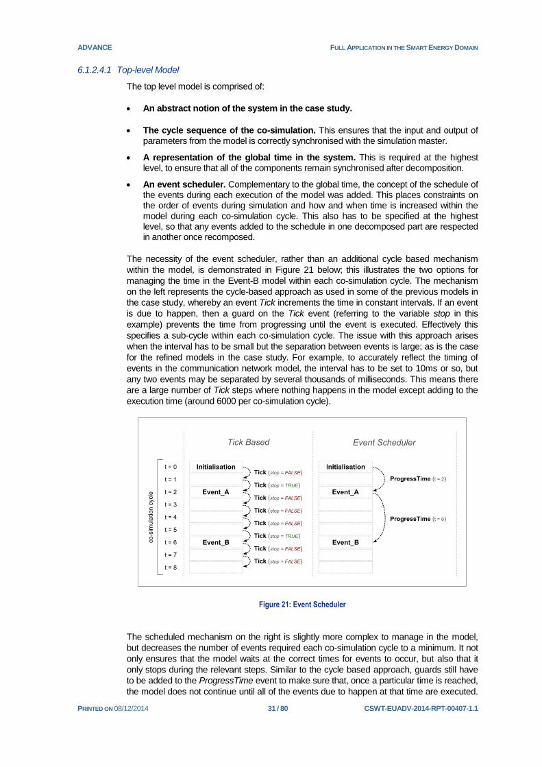
6.1.2.4.1 Top-level Model
The top level model is comprised of:
An abstract notion of the system in the case study.
The cycle sequence of the co-simulation. This ensures that the input and output of parameters from the model is correctly synchronised with the simulation master.
A representation of the global time in the system. This is required at the highest level, to ensure that all of the components remain synchronised after decomposition.
An event scheduler. Complementary to the global time, the concept of the schedule of the events during each execution of the model was added. This places constraints on the order of events during simulation and how and when time is increased within the model during each co-simulation cycle. This also has to be specified at the highest level, so that any events added to the schedule in one decomposed part are respected in another once recomposed.
The necessity of the event scheduler, rather than an additional cycle based mechanism
within the model, is demonstrated in Figure 21 below; this illustrates the two options for
managing the time in the Event-B model within each co-simulation cycle. The mechanism
on the left represents the cycle-based approach as used in some of the previous models in
the case study, whereby an event Tick increments the time in constant intervals. If an event
is due to happen, then a guard on the Tick event (referring to the variable stop in this
example) prevents the time from progressing until the event is executed. Effectively this
specifies a sub-cycle within each co-simulation cycle. The issue with this approach arises
when the interval has to be small but the separation between events is large; as is the case
for the refined models in the case study. For example, to accurately reflect the timing of
events in the communication network model, the interval has to be set to 10ms or so, but
any two events may be separated by several thousands of milliseconds. This means there
are a large number of Tick steps where nothing happens in the model except adding to the
execution time (around 6000 per co-simulation cycle).
Figure 21: Event Scheduler
The scheduled mechanism on the right is slightly more complex to manage in the model,
but decreases the number of events required each co-simulation cycle to a minimum. It not
only ensures that the model waits at the correct times for events to occur, but also that it
only stops during the relevant steps. Similar to the cycle based approach, guards still have
to be added to the ProgressTime event to make sure that, once a particular time is reached,
the model does not continue until all of the events due to happen at that time are executed.

ADVANCE FULL APPLICATION IN THE SMART ENERGY DOMAIN
PRINTED ON 08/12/2014 32 / 80 CSWT-EUADV-2014-RPT-00407-1.1
However, an additional set is also added to the model representing the schedule of events,
which is used by the ProgressTime event to determine by how much the time should be
increased. Events can be dynamically added to this set through the event AddToSchedule:
Figure 22: AddToSchedule event
The AddToSchedule event is brought down into each decomposed part; any new events
which cause something else to happen in the future refine this event. As they all refine the
same top level event, each will be acting on the same schedule variable. This ensures that
the subsystem models will all be synchronised once they are recomposed, and is the
reason why it is imperative to define this scheduling mechanism at this abstract level, before
any decomposition.
6.1.2.4.2 Decomposition of the Top-level Model
The first decomposition step separates out a sub-model containing the model elements
related to the synchronisation of the model with the co-simulation cycle. Effectively this
separates out any timing-related constructs which are specific to the co-simulation setup,
and therefore not directly applicable to the system model. This means that, once separated,
the system model will have no visibility of the cycle behaviour of the co-simulation; it will just
see the time as continuous. However, as the co-simulation constraints have been defined
prior to decomposition, it provides a guarantee that the system model will be compatible with
these constraints once it is recomposed, regardless of the refinement to the system model
[RD-1].
Unlike the other decomposition steps, which split the model into its physical subsystems,
this is an example of using the decomposition process to remove model constructs of which
no visibility is required for the rest of the development. It simplifies the development of the
remaining model by providing a cut-down abstraction to use as a starting point.
6.1.2.4.3 Decomposition into the Cyber subsystems
The system model is first decomposed by separating out the algorithm subsystem, leaving
an abstract notion of a monitoring network which passes values from the low voltage
network to the algorithm. After some refinement, this monitoring network is further
decomposed into the communication network and SIUs. This was seen as the most intuitive
approach, as the communication network and SIU models are more closely linked due to
the additional feedback loop between them. Therefore the algorithm model is separated out
first, leaving this relationship to be developed further before decomposing again.
There are two decomposition processes available in the toolset:
1. Shared Variable Decomposition: The events are manually partitioned between the
subsystems, and the variables are automatically assigned to each subsystem during
the decomposition depending on the events they are referenced in.
event AddToSchedule any event_time where event_time ∈ current_time ‥ END_TIME then schedule ≔ schedule ∪ {event_time} end

ADVANCE FULL APPLICATION IN THE SMART ENERGY DOMAIN
PRINTED ON 08/12/2014 33 / 80 CSWT-EUADV-2014-RPT-00407-1.1
Figure 23: Shared variable decomposition
2. Shared Event Decomposition: The variables are manually partitioned between the
subsystems, and the events are automatically assigned to each subsystem during the
decomposition depending on the variables they reference.
Figure 24: Shared event decomposition
In either case, the events may be partitioned between the decomposed parts:
For shared variable decomposition, this will occur if two events in different subsystems
refer to the same variable. In this case, an external event is added to other subsystems

ADVANCE FULL APPLICATION IN THE SMART ENERGY DOMAIN
PRINTED ON 08/12/2014 34 / 80 CSWT-EUADV-2014-RPT-00407-1.1
that can modify the same variable, as shown in Figure 23. The limitation to this
approach is that external events cannot be refined, to ensure they remain consistent
across subsystems.
For shared event decomposition, it may be that part of an event refers to a variable in
one subsystem and another part refers to a variable in a different subsystem. In this
case, the event is split between the subsystems, as per Event C in Figure 24. The
guards and actions of the event are split between the subsystems depending on which
variables they reference. The limitation in this case is that any guards and actions have
to be disjoint in terms of the variables allocated to different subsystems; i.e. a single
guard or action cannot simultaneously refer to variables in more than one subsystem.
This process of partitioning the events is performed automatically in both cases by the plug-
in.
The shared event approach was used exclusively during the decomposition in Figure 20.
This was partly as the limitations of the shared variable approach were found to have a
more significant impact on the ease of development than the limitations of the shared event
approach. It was easier to adjust the models to work around the fact that guards and actions
in partitioned events have to be disjoint, than it was to structure the models so that all of the
necessary refinements could occur without refining partitioned events. In addition, when
working with system models, shared event decomposition provided a more intuitive result. In
this case, the events which are partitioned clearly represent the interfaces between the
subsystems, and the events which are confined to a single subsystem represent internal
processes. This provides a clear indication of how the different subsystems will interact as a
result of the system design. As an example, consider the automatic split of events during the
decomposition of the monitoring network, as shown in Figure 25 below.
Figure 25: Decomposition of the monitoring network model
Some examples of the internal events of the decomposed models are shown on the far left
and right. The shared events in this case are the SendReport event, where a SIU issues a
report to the communication network, and the AcknowledgementReceived event, which
notifies the SIU if an acknowledgement is received for the report. These shared events
(more specifically, the parameters of the shared events) formalise the interface between the
subsystems. If the models are produced early on, this formalisation can be taken forward to
help define the interfaces for the implementation phases.

ADVANCE FULL APPLICATION IN THE SMART ENERGY DOMAIN
PRINTED ON 08/12/2014 35 / 80 CSWT-EUADV-2014-RPT-00407-1.1
6.1.3 Subsystem Model Development
Moving to the new decomposition-based structure during the recent phase of work required
some changes to the existing models for the algorithm, communication network and SIUs,
to ensure consistency with the other models alongside or higher up in the decomposition
chain. This mostly involved refactoring the existing model elements rather than adding new
components, therefore a large proportion of the existing models could be reused. This
refactoring involved:
Making sure any formal constructs introduced by the models refined the more abstract
constructs introduced higher in the decomposition; i.e. those in the top-level or abstract
system and monitoring network models.
Adjusting the variables, and guards and actions in events, to allow for a clean
decomposition at each step in the process. The structuring of the variables, and
partitioning of the guards and actions in each event, has to be performed in a particular
manner for the decomposition to be both possible and provide the intended result. This
requires some experience with the plug-in, and is discussed further in Section 7.
It is important to define the overall decomposition and refinement structure early in the modelling, otherwise rework is required through
each level.
In addition to this refactoring, some further refinements were made to the communication
network and SIU models during this phase of work, to add the necessary detail for a full co-
simulation. These changes are described in the sections below, along with some additional
explanation on how the previously defined strategy for modelling the communication
protocols was integrated into the decomposition.
6.1.3.1 Communication Network
6.1.3.1.1 Overview
In the previous phase of work [AD-3] two candidate communication topologies between the
SIUs and the algorithm were laid out and modelled. These were:
1. Direct point-to-point communication from each SIU to the algorithm, using a GPRS link
or similar.
2. A wireless mesh topology where each of the SIUs can act as an intermediate hop to the
substation where the algorithm is housed.
As per the last phase, the majority of the rework and refinement was performed on the mesh
topology model. This was due to the higher complexity of the models required to verify the
algorithm against the mesh protocol compared to the point-to-point abstraction. This
development consisted of:
Refining the models so that acknowledgements are generated at the substation end of
the network and routed in the opposite direction to reports. This supported the
retransmission and priority mechanisms added as part of the parallel refinement to the
SIU models.
Integrating the step-wise strategy previously used for modelling the communication
protocols into the decomposition.

ADVANCE FULL APPLICATION IN THE SMART ENERGY DOMAIN
PRINTED ON 08/12/2014 36 / 80 CSWT-EUADV-2014-RPT-00407-1.1
Incorporating the real network topology into the models. For the initial, more generic,
protocol models, the topology was defined in an abstract manner. These models were
refined with further constraints so that they represented the actual network under
consideration in the case study.
Improving how the route calculation and dynamic nature of the mesh protocol were
modelled, to increase the efficiency of the simulation of the model. As the models were
developed – and in particular, when the real topology was imported – the efficiency of
the simulated models in isolation was reduced to a point where it had an adverse effect
on the viability of running a full day in the co-simulation. A fairly substantial amount of
effort, and several iterations of the models, was involved in overcoming this issue.
The integration of the previous modelling strategy for communication protocols, and the
rework involved with improving the efficiency of the simulation of the models, are covered in
more detail in the respective sections below.
6.1.3.1.2 Integration of Previous Models
In the previous phase of work, a generic strategy for modelling communication protocols in
Event-B was developed, with reusable models as an output (see [AD-3]). This strategy was
used to create models for both the point-to-point and mesh topologies. In the original co-
simulation setup (Figure 16), these models could be used directly by replacing the
communication network block with the chosen topology. The same model elements were
reused in the decomposition, however as mentioned some refactoring of the models was
involved to ensure they were consistent with the new structure. The integration of the mesh
topology models into the decomposition chain (Figure 20) is depicted in Figure 26.

ADVANCE FULL APPLICATION IN THE SMART ENERGY DOMAIN
PRINTED ON 08/12/2014 37 / 80 CSWT-EUADV-2014-RPT-00407-1.1
Figure 26: Integration of communication model
As a reminder, the strategy put in place during the last phase of work provides a generic
protocol model as a starting point. This can be refined to create models for specific
protocols, although these models are also kept abstract in terms of any specific network
topology or configuration. This means that, once developed, each specific protocol model
can also be reused by refining it into models of different network configurations which use
the protocol. The corresponding model chain for the mesh topology is shown on the left-
hand side of Figure 26. The generic and mesh protocol models were originally developed
during the previous phase of work. As mentioned earlier in the section, the last model in the
sequence – in which the specific network topology for the case study is introduced – was
added during the latest phase of work.
The integration of this modelling chain into the decomposition structure spans over the
abstract monitoring network and subsequently decomposed communication network
elements. The generic protocol model introduces the abstract notion of packets and the data
payload, in addition to the source and destination of each packet and the schedule for
packet transmission and receipt. The reason this generic model has to be spread over the
two components is that the monitoring network component requires an abstract notion of the
data payload of each packet before it can be decomposed. This has to be defined prior to
the split so that the consistency between the communication network (which transmits the
packet) and the SIUs (which provide or receive the contents of the packet) is maintained.

ADVANCE FULL APPLICATION IN THE SMART ENERGY DOMAIN
PRINTED ON 08/12/2014 38 / 80 CSWT-EUADV-2014-RPT-00407-1.1
The remainder of the generic model is included at the start of the communication network
element, as the remaining elements are specific to this subsystem.
To ensure consistency with the rest of the system, the implementation of the network
schedule in the generic model was also replaced largely by the event scheduler in the top-
level model (see Section 6.1.2.4). This did not induce any significant change overall, as the
concept in both cases is extremely similar. Mostly it was just a case of making sure the
relevant events refined AddToSchedule (Figure 22).
The original model for the mesh protocol and the newly refined model for network topology
could then just be integrated as direct refinements within the communication network
element. Therefore, the decomposition structure does not remove the ability to switch the
specific protocol or network configuration models – for instance, these models can be
substituted to simulate the point-to-point topology instead. As with the other models,
however, these still need to be refactored so they are consistent with the new structure
imposed by the decomposition.
6.1.3.1.3 Simulation Efficiency
The routing protocol used by the mesh network is dynamic; it continually recalculates the
most desirable route from each source and hop depending on a variable cost associated
with each link. This link cost is calculated from a number of parameters, including the uptime
and traffic throughput of each link. Representing this behaviour in Event-B was challenging;
although the greatest challenge was not in creating a viable formal representation, but in
creating a representation which resulted in efficient simulation of the model. The different
iterations of the model before a successful solution was found are described in the following
subsections.
6.1.3.1.3.1 First Iteration
Initially, complex guards were added to each event associated with sending packets. These
guards represented the criteria used by the algorithm to select the most suitable route. This
was a concise and intuitive representation of the logic of the routing protocol, and meant that
the only valid parameters which each event could be executed with were those which would
be chosen by the protocol. However, these parameters still had to be determined by the
simulation tool – ProB – each time the events were executed. This became an issue once
the real network topology was introduced, as the number of potential parameters that ProB
had to search through each time increased dramatically, to a point where it was either too
time-consuming or just infeasible to find a valid combination. It was clear at this point that
this was not a scalable solution.
6.1.3.1.3.2 Second Iteration
In an attempt to separate out the complexity inherent in the guards, the computation of the
most desirable routes was separated out into multiple events. Each time a change occurred
in the network, a series of events were triggered which would re-compute the routes on a
hop-by-hop basis propagating outwards from the source of the change. This was in fact a
closer representation of how the protocol disseminates routing updates throughout the
network. In this case, the parameters for each event were found in a reasonable time.
However, it introduced a different scalability issue; that being, as the complexity of the
network topology increases, so does the number of events associated with each change,
and hence so does the time required for simulation.
The addition of these hop-by-hop updates also increased the complexity of the model and,
although not incorrect, started to take away from the power brought by the formal
abstraction of Event-B. The previous iteration effectively assumed that this propagation of
routing updates is instantaneous; however, considering the time these updates take to
propagate compared to the time step in the model, this is in fact a valid assumption. One of
the main benefits of Event-B is the ability to look at the entire system from an abstract

ADVANCE FULL APPLICATION IN THE SMART ENERGY DOMAIN
PRINTED ON 08/12/2014 39 / 80 CSWT-EUADV-2014-RPT-00407-1.1
perspective, and only focus on the aspects which really matter in terms of the properties to
be verified. In this case additional detail was being added to the model which had no impact
on the verification, but still added to the complexity and simulation time.
6.1.3.1.3.3 Third Iteration
The third – and ultimately successful – approach was to split the calculation of the most
desirable routes into two phases. Before the model is simulated, the network topology is
loaded into a separate Event-B model, which has the sole purpose of computing the subset
of valid routes. This subset is generated by loading the model into ProB, and using the
model checking capabilities to cycle through the potential link combinations in an iterative
fashion (similar to the algorithm employed by the routing protocol). The valid routes are then
transferred into the main model as a constant, which the events refer to when calculating the
most desirable route.
Here the subset of valid routes refers to routes which are legal in terms of the routing
protocol – e.g. routes without any loops. In the first iteration of the model, this legality was
specified by the constraints in the guards. This meant that when finding valid parameters for
each event, every single link combination – legal route or not – had to be considered. Here,
this legality has already been computed, and it is only a case of selecting the most desired
route (i.e. the route with the minimum link cost) from the subset of legal routes. This subset
is far smaller than the entire set of possible link combinations, which if loops are considered,
can in fact be infinite. Obviously there is still a scalability consideration, as the time required
to find all of the valid routes through the model checker will increase with the complexity of
the network topology. However, as the valid routes are pre-computed before the simulation,
this increase in complexity is not compounded by the number of simulated events.
6.1.3.2 SIUs
The SIU models also underwent further development during the recent phase of work,
consisting of:
Integrating the models into the decomposition chain. As with the other models,
some refactoring was necessary to ensure the models were consistent with the more
abstract decomposition elements. The most significant change was moving from a set
of models, each representing an individual SIU, to a single model representing all SIUs.
As it was necessary to introduce an abstract set of SIUs earlier in the decomposition
process, this single model was the natural result of decomposing the monitoring
network element. In most cases this change comprised of switching from variables to
sets (with each set representing a map from SIU to variable).
Further decomposing the SIUs element in Figure 20 into individual SIUs is theoretically
possible, although it would offer no advantages. To ensure consistency with the levels
above, duplicate events would have to be created prior to decomposition. This means
the exact number of SIUs would have to be known beforehand – thereby losing the
flexibility of being able to configure this dynamically in the models by changing the value
of a single variable in the final refinement.
Introducing the retransmission mechanism of the SIUs into the models. In parallel
to the refinement of the communication network model to cater for acknowledgements,
the automatic retransmission mechanism within the SIUs was added to the models. The
transmission of each report is repeated if an acknowledgement is not received after a
set time. If a SIU loses communication with the substation for longer periods of time, it
will also create a backlog of reports and send these at a higher frequency once
communication is restored.

ADVANCE FULL APPLICATION IN THE SMART ENERGY DOMAIN
PRINTED ON 08/12/2014 40 / 80 CSWT-EUADV-2014-RPT-00407-1.1
This behaviour of storing up a backlog of reports to transmit, if not managed carefully
would mean that if the backlog was significant, then it would take a long time to clear,
effectively preventing the algorithm from receiving any values from the SIU. To avoid
this issue, the SIUs use a process known as priority reporting. This involves interrupting
the backlog with a fresh report at regular intervals.
In line with moving to a more concrete model of the communication network where
packet loss is possible, it was necessary to introduce this behaviour as it has a potential
effect on both the operation of the algorithm and the level of network traffic.
6.1.4 Low Voltage Network
The purpose of the low voltage network models is primarily to validate the formal models of
the system. Moreover, when combined with the co-simulation they provide a means to
explore the behaviour of the system under suboptimal operating conditions, such as:
When parts of the communications network fails for extended periods of time;
this can help inform what level of packet loss is acceptable, or what parts of the
communication network contribute to packet loss (e.g. a bottlenecks).
When input voltage is not stable, or consumer demand is the worst case; this in
turn allows exploration of the model behaviour under exceptional conditions or
situations close to the operational limits, which may not be seen during field trials or
even the typical operational lifetime of a specific deployment of the system.
Co-simulation allows for exploration of the formal model’s behaviour under nominal, suboptimal or exceptional situations.
Since the progress reported in deliverable D.2.3 [AD-3], the Modelica models of the
environment have not substantially changed in terms of semantics. However, they have
been scaled up to a realistic size. This includes doubling the number of feeders, from 3 to 6
(i.e. 13 SIUs instead of 7 SIUs), and using a realistic number of houses for each feeder
based on scheme plans provided by Selex ES. The low voltage network models that have
not changed since the previous deliverable are not repeated here, and include: the tap
changer, stochastic determination of communications network outages, and medium
voltage simulation.
The following subsections describe the scaling up of the Modelica models to a
representative topology of the low voltage network, and the changes to the end user
simulations to produce realistic inputs to drive the co-simulation.
6.1.4.1 Topology Scaling
The following provides a top down overview of the Modelica models. Figure 27 shows a
rolled-up view of the low voltage network. The block on the top left generates an input signal
that simulates the medium voltage input into the low voltage network. Within the substation
boundary the OLTC transformer and tap changer are located. The L2L block measures the
three phase line-2-line voltage. The blue triangle in the middle of the substation indicates the
input port for the target voltage, and will be connected to the algorithms output port. The
output from the tap changer block (right most block of the substation) is connected to the
transformer, and selects the discrete tap position.

ADVANCE FULL APPLICATION IN THE SMART ENERGY DOMAIN
PRINTED ON 08/12/2014 41 / 80 CSWT-EUADV-2014-RPT-00407-1.1
Modelica provides an ideal graphical block language for modelling complex systems, which helps ensure the model’s validity.
The output from the transformer is then connected to 6 feeders, each of which is three
phase. The feeders represent the power transmission lines and consumer load and
generation.
Figure 27: Low Voltage Network, Rolled-Up View
Each feeder of the 6 feeder models in Figure 27 is responsible for splitting the three phases
up into three single phases, and connecting up the mid- and end-point SIUs to the
voltmeters in the single phase feeder models. The three phase feeder model is depicted in
Figure 28, where the blue circle at the top is the same blue circle that is on the top left of
each of the feeders in Figure 27. The power flows in at the top, and is split into three
different single phase feeders, which are connected to the SIUs. The output of these SIUs
(white triangles at the base of the blocks) is connected to the Event-B model of the mesh
network. This is implemented textually as Modelica code, and hence is not graphically
depicted.

ADVANCE FULL APPLICATION IN THE SMART ENERGY DOMAIN
PRINTED ON 08/12/2014 42 / 80 CSWT-EUADV-2014-RPT-00407-1.1
Figure 28: Three Phase Feeder
Each of the single phase feeder lines in Figure 28 is implemented as shown in Figure 29.
These models represent two contiguous blocks of houses, each connected by a
transmission line. The voltage is measured at two points on the feeder, once before the first
block of houses, and once before the last block of houses. Although this positioning might
seem counter intuitive, each of the power transmission lines has resistance, capacitance,
and inductance properties, that by applying the laws of electromagnetism means that a
voltage drop is observed at these positions when a load is being drawn by the houses.

ADVANCE FULL APPLICATION IN THE SMART ENERGY DOMAIN
PRINTED ON 08/12/2014 43 / 80 CSWT-EUADV-2014-RPT-00407-1.1
Figure 29: Single Phase Feeder
Each block of houses is implemented as a load and current source (using blocks from the
Modelica standard library), which represent the aggregated load and generation capacity of
the block of houses. In order to ensure the simulations are representative, these loads and
current sources vary throughout the simulation, and are defined by the end user simulation.
6.1.4.2 End User Simulation
The end user simulation has not substantially changed since the last deliverable D.2.3 [AD-
3]. It is still based on the models produced by the CREST project [RD-2], and Modelica
models are generated that represent instances of the simulation. What has changed since
the previous deliverable are the parameters that configure the CREST model; this is to
provide more realistic simulations to improve the quality of the co-simulation. This included:
Determining the numbers of houses on each beginning-mid and mid-end point
segments of each of the 6 feeders.
Looking up statistics from the Office of National Statistics (UK) to determine the
distribution of household sizes, and the distribution of sizes (in kW) of PV panels.
It should be noted that the intention was not to provide an exact representation of the
network in the case study, but to generate a more realistic model that could in turn be varied
to validate the system operation against a wider range of more realistic scenarios.

ADVANCE FULL APPLICATION IN THE SMART ENERGY DOMAIN
PRINTED ON 08/12/2014 44 / 80 CSWT-EUADV-2014-RPT-00407-1.1
6.1.4.2.1 Household Counting
Determining the numbers of houses on each segment of each feeder was accomplished by
examining the scheme plan and manually counting the houses. Figure 30 shows a
simplified version of the scheme plan, overlaid on the map of the area, where the black
circles indicate the mid points, and the white circles indicate the end points. Notice that the
actual feeder layout and the models presented previously diverge in that the feeders are not
necessarily linear. However, for the purposes of this case study it was agreed with Selex ES
that the linear modelling that was applied would suffice. Moreover, the actual scheme plan
cannot be made publically available. With respect to this work, the only detail from the
scheme plans not depicted in Figure 30 are which houses are connected to which phases.
Figure 30: Feeder Layout
For each feeder, there is a mid- and end-point measurement, and each measurement
consists of three phases. Thus, the table in Figure 31 was produced from the plan, which
was used to generate a Modelica model that represents the end user simulation model as
discussed in [AD-3]. The table in Figure 31 assigns the PV penetration to each of the
segments of each feeder; this value is the probability that a given house in that segment will
have a PV panel installed. There were no statistics available to concretely identify the PV
distribution for the site in Figure 30, so these numbers were selected to provide an
interesting distribution where some feeders have more PV than others.
The first row of the table states: phase 1 of the beginning-midway segment of feeder 1 has 1
house, with a 50% probability that it will have a PV panel installed.
Phase PV Penetration No of Houses
Feeder 1 Mid P1 0.5 1
P2 0.2 2
P3 0.2 1
End P1 0.2 7
P2 0.2 4
P3 0.2 6
Feeder 2 Mid P1 0.5 8
P2 0.3 6
P3 0.7 9

ADVANCE FULL APPLICATION IN THE SMART ENERGY DOMAIN
PRINTED ON 08/12/2014 45 / 80 CSWT-EUADV-2014-RPT-00407-1.1
End P1 0.2 15
P2 0.2 14
P3 0.1 13
Feeder 3 Mid P1 0.5 14
P2 0.7 15
P3 0.5 14
End P1 0.2 17
P2 0.2 16
P3 0.2 20
Feeder 4 Mid P1 0.5 15
P2 0.2 6
P3 0.2 2
End P1 0.2 7
P2 0.2 9
P3 0.2 6
Feeder 5 Mid P1 0.5 9
P2 0.3 8
P3 0.7 9
End P1 0.2 5
P2 0.2 4
P3 0.1 10
Feeder 6 Mid P1 0.5 15
P2 0.7 12
P3 0.5 15
End P1 0.2 19
P2 0.2 14
P3 0.2 12
Figure 31: House Statistics
To illustrate the above model, the mid-point plot of phase 1 of feeder 3 (black feeder in
Figure 30) is shown in Figure 32. The plot shows the aggregated consumption (active and
reactive) and generation of a block of 14 houses, where 6 houses had PV panels.

ADVANCE FULL APPLICATION IN THE SMART ENERGY DOMAIN
PRINTED ON 08/12/2014 46 / 80 CSWT-EUADV-2014-RPT-00407-1.1
Figure 32: Feeder Plot
6.1.4.2.2 Statistics
The model developed by CREST is parameterised by the number of occupants in the
house, which is between 1 and 5 inclusive. The number of occupants is used to select a
probability distribution, which is used to generate the number of active occupants in a house
throughout the day. The active occupants feed into when appliances and lights are active.
To ensure these numbers were realistic for the simulations, the probability distribution of the
number of occupants in a house was obtained from the 2011 census data [RD-6] and an
updated estimate in [RD-5]. The distribution obtained is depicted in Figure 33.
Figure 33: Household Size Distribution (2011 Census)
The distribution in Figure 34 is used to determine the generation capacity of the PV panels.
It is based on the FiT statistics available from the Department of Energy & Climate Change,
UK [RD-7].
0.00%
10.00%
20.00%
30.00%
40.00%
1 2 3 4 5+
Household Size Distribution

ADVANCE FULL APPLICATION IN THE SMART ENERGY DOMAIN
PRINTED ON 08/12/2014 47 / 80 CSWT-EUADV-2014-RPT-00407-1.1
Figure 34: PV Generation Distribution
It was investigated what the likelihood of a house having a PV panel installed was, which
was obtained by taking the total number of sub 4kW PV installations over the number of
dwellings in the UK, which is:
50824223366044⁄ ≈ 2.1%
However, this would not have provided good simulation results as the case study is targeted
towards areas where there are a high number of PV installations. For this reason, it was
decided to allow for the PV distribution to be directly specified for each phase of each
segment of each feeder separately. This would in addition allow for investigating realistic
scenarios where some parts of the network have disproportionally high PV penetration.
0.00%
10.00%
20.00%
30.00%
40.00%
1 2 3 4
PV Distribution (sub 4kW)

ADVANCE FULL APPLICATION IN THE SMART ENERGY DOMAIN
PRINTED ON 08/12/2014 48 / 80 CSWT-EUADV-2014-RPT-00407-1.1
6.2 Co-Simulation
The co-simulation reported in the previous deliverable was a proof of concept to evaluate
the methodology. It did not include the full communication network model, nor the stochastic
model of the communications link failures, and only contained half the required SIUs.
Also reported on in the last deliverable were the inefficiencies of the underlying toolset that
were experienced on the small scale proof of concept. These inefficiencies were raised with
the ADVANCE consortium, and in particular, with the Universities of Düsseldorf (UDUS) and
Southampton. In response to this, UDUS improved the underlying implementation of the
ProB tool to mitigate the inefficiencies experienced.
During the final phase of the case study, substantial focus has been on trying to get the co-
simulation running efficiently for an entire day. A 24 hour period was selected for the
simulation as this would validate the solution against a realistic scenario, with the current
peaks and troughs in realistic locations – that is, peaking in the morning around breakfast
time and again during the evening with a trough during midday when there is PV
contribution. This has involved undertaking investigations into which parts of the framework
suffer from efficiency issues, and the best ways to avoid these issues. Part of this involved
restructuring the formal models, as explained further in Section 6.1.2.
6.2.1 Experiment: SIUs into Modelica
In order to understand whether the Event-B or Modelica models were causing the
inefficiencies during the simulations, the abstract models of the SIUs from the previous
phase were refactored into Modelica models. The simulation setup as previously presented
in [AD-3] is repeated in Figure 35.
Figure 35: Component Diagram from D.2.3 [AD-3]
In Figure 35, the machine R9_fmi_state is a model of the algorithm, and the R2_intervals
machines are abstract models of the SIUs and communications. In this test, the SIUs take
inputs from the continuous model every 0.5 time steps (i.e. 30 seconds) and averages them
over 1 time step (i.e. 1 minute), then report these averaged values to the algorithm. The

ADVANCE FULL APPLICATION IN THE SMART ENERGY DOMAIN
PRINTED ON 08/12/2014 49 / 80 CSWT-EUADV-2014-RPT-00407-1.1
algorithm takes these averaged values every 5 time steps (i.e. 5 minutes) and performs
some computation on them to determine a new target, which is fed back to the Modelica
model (i.e. the green block). The values were chosen for the purposes of the experiment,
and do not represent the real reporting and averaging intervals.
The component diagram of the refactored simulation after moving the SIU models into
Modelica is shown in Figure 36. Using the refactored simulation it was possible to evaluate
the entire day using the 30 second time steps (as opposed to only 500 steps as reported in
[AD-3]). Using the refactored simulation, it was also possible to start investigating the
behaviour of the system by viewing the Event-B traces of the algorithm and the plots of
choice variables in the low voltage network, see Figures 37, 38 and 39.
Figure 36: Component Diagram: SIUs in Modelica

ADVANCE FULL APPLICATION IN THE SMART ENERGY DOMAIN
PRINTED ON 08/12/2014 50 / 80 CSWT-EUADV-2014-RPT-00407-1.1
Figure 37: Medium Voltage Input, Nominal ≈6.7kV (kV line-2-neutral)
Figure 38: Busbar and Target Voltage (line-2-line)
Figure 39: Discrete Tap Position
It is clear from this experiment that the underlying inefficiencies are with Rodin and ProB.
When moving the abstract SIU implementation into Modelica the gains were substantial.
The Event-B models of the SIU were simple, and only performed an averaging of the
values, but the number of them, (i.e. 7) and the extra events (read, wait) they required
slowed the simulation down and substantially increased the memory requirements.
As a result of this investigation, it was concluded that the averaging behaviour of the
simulation should be transferred to the Modelica model of the LV network (as shown in
Figure 28). This meant the models could represent the SIUs sampling the underlying
voltage at a higher frequency, i.e. from 30 seconds to 1 second (which is representative of
the real SIUs), whilst increasing the co-simulation step size to 1 minute (from 30 seconds).
That is, the SIUs only produce reports at a 1 minute resolution with averaged
measurements of the voltage; instead of passing instantaneous values from the continuous
to formal SIU models every second, an averaged value is just passed every minute.
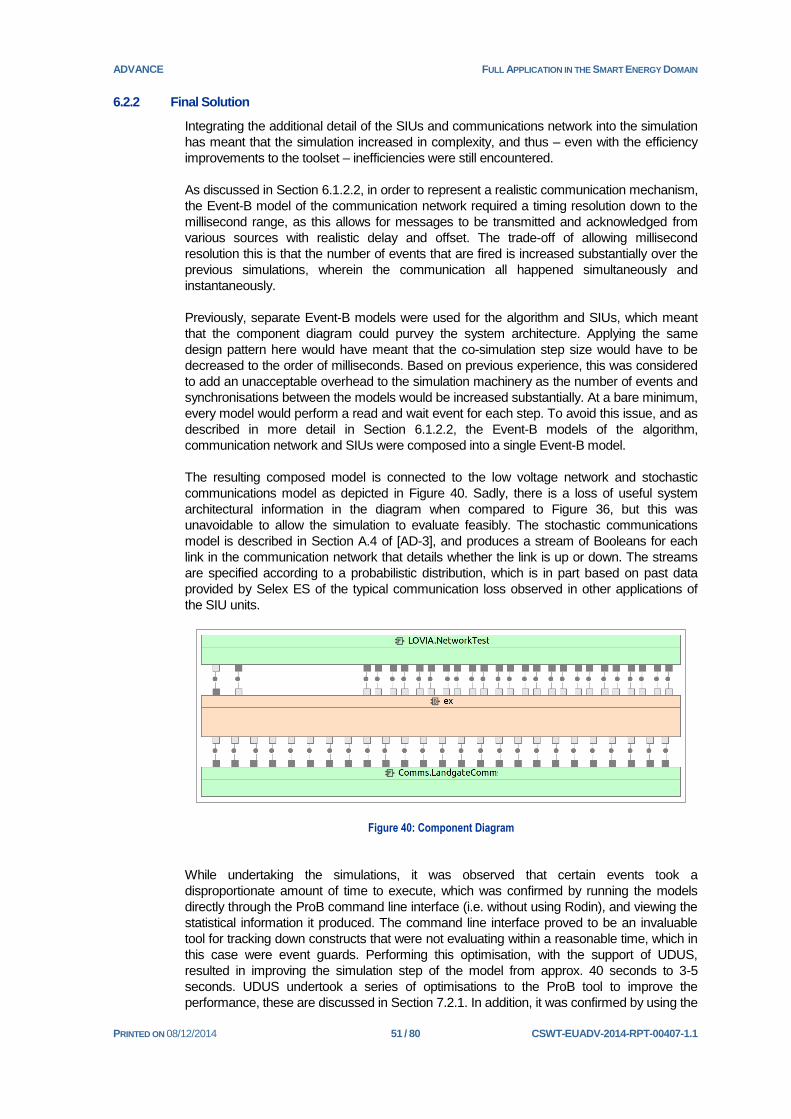
ADVANCE FULL APPLICATION IN THE SMART ENERGY DOMAIN
PRINTED ON 08/12/2014 51 / 80 CSWT-EUADV-2014-RPT-00407-1.1
6.2.2 Final Solution
Integrating the additional detail of the SIUs and communications network into the simulation
has meant that the simulation increased in complexity, and thus – even with the efficiency
improvements to the toolset – inefficiencies were still encountered.
As discussed in Section 6.1.2.2, in order to represent a realistic communication mechanism,
the Event-B model of the communication network required a timing resolution down to the
millisecond range, as this allows for messages to be transmitted and acknowledged from
various sources with realistic delay and offset. The trade-off of allowing millisecond
resolution this is that the number of events that are fired is increased substantially over the
previous simulations, wherein the communication all happened simultaneously and
instantaneously.
Previously, separate Event-B models were used for the algorithm and SIUs, which meant
that the component diagram could purvey the system architecture. Applying the same
design pattern here would have meant that the co-simulation step size would have to be
decreased to the order of milliseconds. Based on previous experience, this was considered
to add an unacceptable overhead to the simulation machinery as the number of events and
synchronisations between the models would be increased substantially. At a bare minimum,
every model would perform a read and wait event for each step. To avoid this issue, and as
described in more detail in Section 6.1.2.2, the Event-B models of the algorithm,
communication network and SIUs were composed into a single Event-B model.
The resulting composed model is connected to the low voltage network and stochastic
communications model as depicted in Figure 40. Sadly, there is a loss of useful system
architectural information in the diagram when compared to Figure 36, but this was
unavoidable to allow the simulation to evaluate feasibly. The stochastic communications
model is described in Section A.4 of [AD-3], and produces a stream of Booleans for each
link in the communication network that details whether the link is up or down. The streams
are specified according to a probabilistic distribution, which is in part based on past data
provided by Selex ES of the typical communication loss observed in other applications of
the SIU units.
Figure 40: Component Diagram
While undertaking the simulations, it was observed that certain events took a
disproportionate amount of time to execute, which was confirmed by running the models
directly through the ProB command line interface (i.e. without using Rodin), and viewing the
statistical information it produced. The command line interface proved to be an invaluable
tool for tracking down constructs that were not evaluating within a reasonable time, which in
this case were event guards. Performing this optimisation, with the support of UDUS,
resulted in improving the simulation step of the model from approx. 40 seconds to 3-5
seconds. UDUS undertook a series of optimisations to the ProB tool to improve the
performance, these are discussed in Section 7.2.1. In addition, it was confirmed by using the

ADVANCE FULL APPLICATION IN THE SMART ENERGY DOMAIN
PRINTED ON 08/12/2014 52 / 80 CSWT-EUADV-2014-RPT-00407-1.1
command line interface that it was possible to evaluate the model for thousands of steps,
which in informal tests appeared to require linear time with respect to the number of events
animated.
6.2.3 Hardware Resources needed for Analysis
With the observed evaluation of the Event-B models through the ProB command line
interface, and the improvements to the underlying framework, it was assumed that the
simulations would evaluate efficiently. That is, roughly 5 * 1440 seconds, or 2 hours.
However, this was not observed when running the simulation through Rodin. Using a
computer with 16GB memory to run the co-simulation as in the previous deliverable,
approximately 150 (out of a target of 1440) steps were achieved before running out of
resources. However, observing the resource usage for these simulations appeared to be
roughly linear, and the exponential curves reported in [AD-3] were not observed. Thus, it
was hypothesised that running the simulation for an entire day would require roughly 120GB
memory. However, the initial dataset of 150 steps was not enough to adequately predict the
underlying complexity of the simulation, as discussed below.
To test this hypothesis, the use of an Amazon Web Services (AWS) server was employed.
Renting a server with 244GB RAM (the largest currently available) could complete 650
simulation steps, i.e. less than 50% of the desired 1440 steps. The results of the memory
usage are plotted in Figure 41, where x-axis is actual time, not simulated time. From this, it
was clear that the bottleneck was with the Rodin platform, which consumed 90+% of the
system RAM, and appears to have an exponential memory requirement. Whereas, the ProB
command line interface consumed less than 4% of the RAM, and appeared to have a
logarithmic memory footprint. Figure 42 shows the time each step took within the simulation,
and that there is an approximate factor of 10 increase in time when compared to only using
the ProB command line tool to animate the models.
Figure 41: AWS Memory Usage

ADVANCE FULL APPLICATION IN THE SMART ENERGY DOMAIN
PRINTED ON 08/12/2014 53 / 80 CSWT-EUADV-2014-RPT-00407-1.1
Figure 42: Time per Simulation Step
In conclusion, it was observed that the increase in time was due to the way that the
co-simulation framework was calling the ProB command line interface. Namely, that it was
only calling the interface to execute a single event, then checking to determine whether the
simulation step was over, and if not repeating for the next event. This swapping between
Rodin and ProB for each event was causing substantial efficiency problems. To put this in
scale, the experiment that is described in Figures 41 and 42 had approximately 170K
events. The results of these tests were reported back to UOS and UDUS, along with the
suggestion that it would be ideal for the co-simulation framework to delegate as much work
as possible to the ProB command line interface to reduce this switching between tools.
6.2.4 Optimised ProB
In late October 2014 UDUS finished modifying ProB to expose a new command from its API
that does exactly this (cf. ExecuteUntil command). It starts animating the model, and
iteratively executes events until a given formula holds (or a timeout occurs). Once this
formula holds, e.g. when the guards of a given event become true, control is returned to the
multi-simulation framework – that is, controls stays in the ProB command line interface
during the execution of the Event-B model until the end of the co-simulation step.
This new command, and other general efficiency improvements within the Rodin/ProB
toolset have meant that it is possible to simulate for the desired 1440 steps using a fraction
of the resources and less time. The resource plot of this simulation is shown in Figures 43
and 44 where the test system only had 16GB RAM (compared to 244GB in Figure 41) and
completed in just over 7.5 hours (compared to only getting to less than 50% in 9 hours
Figure 41).

ADVANCE FULL APPLICATION IN THE SMART ENERGY DOMAIN
PRINTED ON 08/12/2014 54 / 80 CSWT-EUADV-2014-RPT-00407-1.1
Figure 43: Optimised ProB
Figure 44: Optimised ProB Simulation Step Time
The simulation detailed above in Figures 43 and 44 generated a trace of 380568 events,
which was saved to disk as used to generate the “first attempt” animations described in
Section 7.2.2. The spikes in the second half of the series in Figure 44 are related to the
communications network outages: When link fails, the SIU keeps trying to retransmit data,

ADVANCE FULL APPLICATION IN THE SMART ENERGY DOMAIN
PRINTED ON 08/12/2014 55 / 80 CSWT-EUADV-2014-RPT-00407-1.1
which results in more events within a given cycle, confer with Figure 46 which has the same
communications failures model.
However, it is possible to improve upon this by not saving the full trace, and only saving the
events that form the deterministic portion of the trace during the synchronisation points. That
is, the read events and their parameters are saved. This is because, by design the state of
the formal models of the system stabilise at the end of a simulation cycle; within each cycle
the events fire in a non-deterministic pattern, but at the end of the cycle the state of the
model converges regardless of the order of the events within the cycle. Thus, it is possible to
replay an isomorphic trace of the simulation, where the states of the two traces are the
same whenever a read event occurs. This resulted in drastically improved performance, and
this simulation took just over an hour to run. The results of this are plotted in Figures 45 and
46. It is clear that without recording the whole trace significant gains are possible.
Figure 45: Optimised ProB and Reduced Bookkeeping

ADVANCE FULL APPLICATION IN THE SMART ENERGY DOMAIN
PRINTED ON 08/12/2014 56 / 80 CSWT-EUADV-2014-RPT-00407-1.1
Figure 46: Optimised ProB with Reduced Bookkeeping Simulation Step Time
Using the co-simulation framework, a number of scenarios have been investigated. The
topology was fixed and based upon one of the actual test sites so Selex ES could compare
the results of this work against tests in the real world. The communications network
stochastic failure model was mutated, by altering the probabilities of a failure. This helped to
elucidate how the system would function with differing levels of packet loss, which helped
elucidate what an acceptable packet loss is whilst maintaining a stable voltage on the
network.
Independently of the communications network mutations, the end-user demand models
were mutated. This has included changing the amount of PV distribution within the feeders
and the medium voltage inputs within the network. In some experiments the medium voltage
was placed near the upper (or lower) legal boundaries. This has helped investigate how the
system responds with different levels of consumer demand and generation.

ADVANCE FULL APPLICATION IN THE SMART ENERGY DOMAIN
PRINTED ON 08/12/2014 57 / 80 CSWT-EUADV-2014-RPT-00407-1.1
6.3 Visualisation
In order to explore the results of the co-simulation, further visualisations were produced in
BMotion Studio. Some simple visualisations of the communication traffic were created
during the last phase of work (see [AD-3]), although a new version of the BMotion Studio
tool has been released since. The previous version of the tool was integrated into Eclipse,
and although this allowed for the visualisation to be run directly alongside the other plug-ins
within Rodin, the diagrams that could be produced were limited in terms of design flexibility,
and inefficient when creating numerous or repeated elements. In order to move away from
these limitations, the new version of the tool operates outside of Eclipse, and allows for
visualisations to be created using JavaScript and other HTML-based technologies. Not only
does this remove the design limitations inherent in the previous version (by allowing any
SVG image to form the base of the visualisation), it also permits a lot more flexibility and
scope in terms of how visualisations are created and executed. For example, existing
JavaScript libraries can be integrated for more efficient development. Visualisations are run
within any browser, and can be scripted; making it easy to share the visualisation with
domain experts without requiring an installation of Rodin. The visualisation, however, is still
linked directly to the underlying Event-B model or simulation trace, so the visualisations are
as faithful as the previous implementation. The visualisation of the network in the previous
and new tools is presented in Figure 47 and Figure 48 respectively for comparison. As can
be seen, the improvements are quite significant.
Figure 47: Previous Communication Network Visualisation

ADVANCE FULL APPLICATION IN THE SMART ENERGY DOMAIN
PRINTED ON 08/12/2014 58 / 80 CSWT-EUADV-2014-RPT-00407-1.1
Figure 48: New Communication Network Visualisation
The semantics of Figure 48 are slightly different to that in the previous visualisation; the level
of network traffic through active links is represented by the shade of green (the more traffic,
the darker the shade) rather than the width, and any inactive links are shown in red. The bi-
directionality of the traffic is also considered. The topology shown in Figure 48 depicts the
physical topology of the network in the case study, rather than just a logical representation
(as depicted in the initial prototype in Figure 47). As before, the visualisation elements are
updated as the model is stepped through.
Visualisation was found to be essential in comprehending the results of the simulation, and understanding why any unexpected or non-optimal
behaviour occurred.
In addition to the communication network, another overlay was added visualising the low
voltage network; this was required in order to understand, and validate, how the algorithm
was reacting to changes in the voltage network. This overlay is shown in Figure 49; the
same node layout is utilised, but with the connections now representing the feeders
between the nodes. The overlays can be switched at any time during the simulation by
interacting with the visualisation.

ADVANCE FULL APPLICATION IN THE SMART ENERGY DOMAIN
PRINTED ON 08/12/2014 59 / 80 CSWT-EUADV-2014-RPT-00407-1.1
Figure 49: Visualisation of the low voltage network
The algorithm categorises each feeder and measurement point through specific bands; the
voltage is considered nominal (green) if it lies within a defined range around 230V. Outside
of this, the voltage is considered sub-optimal (yellow), and further still the voltage moves
outside of the statutory limits (red). The severity of the action performed by the algorithm at
each step is determined by where the different voltage measurements lie within these
bands. This categorisation is directly reflected through the colours of the feeders in the
visualisation.
In terms of the two graphs in the lower right of Figure 49, the graph on the left displays the
voltage over time of the selected point (EP12 in Figure 49). The user can select different
points during the visualisation and the graph will be updated to reflect the data at that
location. Therefore each point can be inspected in more detail if, for instance, the voltage
drops into the red band during operation – as is the case for EP12 in Figure 49. The graph
on the right indicates the tap position at the transformer; in this example, a tap up has just
occurred to mitigate the low voltage on the feeder terminating at EP12.

ADVANCE FULL APPLICATION IN THE SMART ENERGY DOMAIN
PRINTED ON 08/12/2014 60 / 80 CSWT-EUADV-2014-RPT-00407-1.1
7. Conclusions
This section summarises the overall experiences of using the ADVANCE methods and tools
on an industrial scale problem. The section is structured as follows:
7.1 Overall Strategy Adopted and Tools Utilised
7.2 Influence on tool development
7.3 Successes and Benefits
7.4 Failures and Disadvantages
7.5 Review of ADVANCE Methodology by Selex ES
7.6 Lessons Learnt
7.7 Recommendations
7.1 Overall Strategy Adopted and Tools Utilised
This section provides a brief overview of the methodology that was applied during this work
package, and our view on how the ADVANCE workflow complements established
workflows. The goal of the revised case study was to investigate using the ADVANCE
toolset to support Selex ES in designing a voltage control system.
Figure 50 provides – from WP2’s perspective – an overview of how the ADVANCE workflow
relates to the standard software V-model. That is, it is well suited to supporting the activities
analysis and design activities at the top left of the V-model.
Figure 50: ADVANCE V-Model
Within this case study the emboldened elements on the right-hand side of Figure 50 have
been focused on. That is, a safety analysis was performed and the system requirements

ADVANCE FULL APPLICATION IN THE SMART ENERGY DOMAIN
PRINTED ON 08/12/2014 61 / 80 CSWT-EUADV-2014-RPT-00407-1.1
were formalised as Event-B models. The system requirements were verified and validated
by the support of proof tools and the multi-simulation framework. The continuation of the
workflow by system requirements by successive refinements of the Event-B models to
obtain the detailed software requirements was not undertaken in this work, instead the
results of the verification and validation of the system requirements were fed back to
Selex ES who are responsible for the overall solution design.
The workflow undertaken within this case study is best placed onto the V-model in Figure
51, where the activities it describes are actually a breakdown of the activities situated at the
top left of the V-model depicted in Figure 50. The implementation phase refers to creating
detailed Event-B system requirements, and the testing activities on the right-hand side have
been replaced by proving and simulation activities. The use of the V-model is natural in this
circumstance as the created Event-B models are executable specifications of the final
system, and thus, can be executed and debugged early on during the system’s lifecycle.
Figure 51: Case Study Workflow
Workflow in Figure 51 increases the quality of the final system by supporting debugging, formal verification and validation of the
requirements during the design.
The system architecture and requirements were provided by Selex ES as inputs, which the
STPA was performed upon. Applying STPA allowed for an enrichment of the requirements,
and identification of requirements that the software components of the system need to fulfil.
STPA proved invaluable to identify requirements and high-level system architecture.
These requirements were fed into the next phase of using the iUML-B plugin to craft
abstract software architectures which captured the logical sequences of events within the

ADVANCE FULL APPLICATION IN THE SMART ENERGY DOMAIN
PRINTED ON 08/12/2014 62 / 80 CSWT-EUADV-2014-RPT-00407-1.1
models. These abstract machines were refined using Event-B directly (instead of iUML-B),
as it provided the flexibility required. Throughout the development of the Event-B models,
ProB was copiously applied to animate the models, which provided in-situ feedback as to
whether the models appeared to perform the correct functions.
The proof capabilities in Rodin were utilised for several distinct purposes:
To analyse the correctness and consistency of the requirements identified during
STPA and the design provided by Selex ES. This typically involved proving that the
model (representing the design) fulfilled invariants (representing the requirements).
To ensure the models were a valid representation of the system in question. For
example, when the behaviour of the mesh routing protocol was added to the model,
invariants representing the rules and constraints specified in the definition of the
protocol were added. These were not added to analyse the requirements of the
protocol, but instead to ensure the modelled behaviour was a correct representation
of the protocol.
To ensure any model refinement and decomposition was well-formed and
consistent. In some cases these proofs tie into or represent requirement proof. For
instance, demonstrating that two refinement levels are consistent can show that a
set of derived requirements (specified in the refined model) are consistent with the
higher level requirements (specified in the more abstract models).
Theories were also used in conjunction with the proofs, to better handle complex
relationships or larger sets representing realistic topologies or data. Several theories defined
in the standard theory library developed during ADVANCE were utilised successfully in the
case study.
Finally, the simulation phase of the workflow provided the means to validate that the models
fulfilled the requirements furnished by Selex ES in the architecture and requirements.
Visualisations ensured that the results of the simulation could be easily interpreted and
explored.
7.2 Influence on tool development
This section summarises any specific points of feedback provided by WP2 that influenced
the tool development during the course of the case study, along with the resulting changes.
As such, this section does not cover more general feedback in terms of the overall
robustness, scalability, and industry-readiness of the toolset; this is covered later in the
conclusions section.
In addition, numerous smaller bugs and usability issues were reported throughout the
duration of the case study, which are not listed in any detail in this section, but regardless
helped improve the robustness and usability of the tools. The feedback and changes for
each of the tools used during the case study are presented in the following subsections:
7.2.1 ProB (Event-B simulation)
7.2.2 BMotion Studio (visualisation)
7.2.3 iUML-B
7.2.4 Decomposition
7.2.5 Composition
7.2.6 Multi-simulation

ADVANCE FULL APPLICATION IN THE SMART ENERGY DOMAIN
PRINTED ON 08/12/2014 63 / 80 CSWT-EUADV-2014-RPT-00407-1.1
7.2.7 ProR (Requirements management)
7.2.1 ProB
Most of the feedback and changes in terms of ProB were related to smaller issues
encountered when trying to simulate certain constructs (for instance, correcting how
particular function definitions are handled, or determining when sets should be expanded or
left symbolic), or when trying to improve the efficiency of the simulation. The latter was a key
consideration during the later stages of the case study, when the efficiency of the overall co-
simulation required significant improvement. Although the animation performed by ProB is
only a part in the overall co-simulation, both rework of the models and fine tuning of the
animation parameters in ProB was performed. This was to ensure the simulation of the
Event-B models was as efficient as possible within ProB when considered in a standalone
manner. These improvements were performed through a coordinated effort from CSWT and
UDUS, and are summarised by the points below:
Most of the rework to the models focused around the communication network – this is
presented in more detail in Section 6.1.3.1. In summary, the most significant
improvements were found from separating out the computation of complex parameters
into multiple events (each computing sub-parameters), and by pre-calculating as much
detail as possible before simulation by adding this through constants in the model. ProB
contains a profiler which provides the average execution time for each event during the
simulation; this was key to determining exactly which events in the model were creating
the performance bottleneck.
The simulation in ProB was tailored to the case study by enabling particular options or
parameters. For instance, the ‘-execute’ option was utilised, which performs the first
enabled operation it finds at each step (rather than providing random operations) and
doesn’t store the state space, significantly increasing the speed of the simulation. This is
suitable for the case study, as the order of events is mostly deterministic, and there is
no need to know the entire state space between every single event.
During these activities, the underlying ProB framework was also updated, providing
further performance improvements.
Further efficiency issues were also encountered for the overall co-simulation outside of ProB
– i.e. when also considering the communication between ProB and Rodin rather than just
ProB in a standalone manner. These are covered in more detail in Section 6.2.
Alongside these changes and improvements, two other key points were raised as a result of
the work on the case study:
Issue / Feedback Resulting Changes Resolved?
Incompatibilities between the Theory plug-in
and ProB was a serious hindrance to progress:
when dealing with realistic sized sets (for
instance, sets representing routing
configurations or measurement data), there is
often no alternative but to use theories. This
issue was already raised through other work
with the toolset, although the prioritisation to
provide a fix was reinforced by the work on the
case study.
Updates to ProB within Rodin
to handle theory constructs
correctly.
Yes
Update released
during ADVANCE
The quality of the simulation in ProB was found Provide the ability to manually Yes

ADVANCE FULL APPLICATION IN THE SMART ENERGY DOMAIN
PRINTED ON 08/12/2014 64 / 80 CSWT-EUADV-2014-RPT-00407-1.1
to be hindered by the inability to concisely select
the parameters of an event execution. ProB
generates a selection of possible parameter
combinations for each event, but when the
number of possible combinations is particularly
large (e.g. when the parameters represent
measurement data) this is not a practical
approach.
specify the parameters of an
event during ProB simulation
within Rodin, so that specific
paths of interest can be
explored when the number of
possible parameter
combinations is too large to
display a representative
subset.
Mechanism added to
allow additional
predicate for event
parameters
7.2.2 BMotion Studio
As a result of the case study, several improvements to the tool were required in terms of the
efficiency of the visualisation. This was brought about from the combination of:
1. the high number events required to simulate a full day in the simulation (upwards of
300,000), and
2. the requirement to visualise an overview of the entire day in a short period of time.
For smaller models or simulations, the default behaviour of the tool – executing every event
in sequence and updating the visualisation in step – ran at a sufficient speed. However, with
hundreds of thousands of events, this was no longer the case, and the visualisation took
multiple hours to complete. This was also not a suitable approach to what we wanted to
achieve in this instance; as we only wanted to visualise an overview of the behaviour over
an extended period of time, it was sufficient to only update the visualisation, say, every 100
or 200 events.
The first step in resolving this issue was to allow for the visualisation to run from a trace of
events after the simulation, rather than directly during the simulation. The co-simulation is
run separately and outputs a trace once complete; this trace is loaded back into the
visualisation which is run at a later stage. This required the development of a script from
UDUS on the visualisation side, to successfully load and execute the trace. However,
although this separated out the simulation and visualisation, the performance gain was only
slight. This was due to the fact that even though the order of events is pre-calculated – and,
even if the visualisation itself is only updated every 100 or 200 steps – the full trace is still
loaded and re-run through ProB to calculate the state of the variables at each step. Some
further improvements were made to this replay mechanism which considerably decreased
the visualisation time, although this was still an order of magnitude too high to allow for a full
day to be visualised in a reasonable time.
To allow for a more efficient execution of a ‘macro-level’ visualisation, which only updates
once every certain number of steps, it requires that only a subset of the trace is loaded into
the visualisation. Two separate approaches were investigated by CSWT and UDUS to
achieve this:
1. The first approach consisted of producing a bespoke script, which constructed the
state of the variables relevant to the visualisation at particular points, directly from
the full trace. The result represented the state of the chosen variables at the start of
each co-simulation cycle, i.e. once per minute in the simulation. These variable
states could then be loaded directly into the visualisation (without running the model
through ProB), and hence allowed a full day in the simulation to be visualised in
only 1440 steps (rather than several hundreds of thousands) and in around 10
minutes.

ADVANCE FULL APPLICATION IN THE SMART ENERGY DOMAIN
PRINTED ON 08/12/2014 65 / 80 CSWT-EUADV-2014-RPT-00407-1.1
This approach was more of an initial investigation, and was only possible for the
specific models used in the case study as the state of the chosen variables could
be inferred directly from the full trace. For other models, this may not be possible.
As the original trace only contains the events and event parameters, if there is any
non-determinism in the model which affects the values of the chosen variables (or
the variables are not easily calculated from the event order and parameter values),
this is not feasible. It also requires a separate script to be written for each
translation.
2. The second approach, implemented by UDUS, was to utilise some of the efficiency
improvements made to the co-simulation, and only load select events from the
trace into ProB. In this case, only the event at the start of each co-simulation cycle
is loaded from the trace, and ProB is left to execute events in the model until the
end of the next co-simulation cycle. Although the time for the visualisation to
complete was longer than the approach above (around an hour), this was still a
significant improvement from loading each and every event from the trace. It also
has the added benefit that the visualisation can be run in parallel with the multi-
simulation framework.
Again, this approach was only possible for the case study due to the specific
structure of the models. The level of determinism in the models means that, for a
particular set of inputs from the continuous models, the formal model will always
end up in the same state by the end of the co-simulation cycle. Hence, although the
number and order of events can vary during the cycle, it will always reach the same
state by the end of the cycle, and so the visualisation can be confidently replayed at
the macro-level without requiring knowledge of the full trace of events during each
co-simulation cycle. For other models, this will likely not be the case.
It is clear that, although both of these approaches were sufficient for the specific case study,
a more generic approach is required moving forward with the tool. One possible solution
would be to output two separate traces from the co-simulation:
1. The first trace is that currently created by the co-simulation – a list of all the events
executed during the co-simulation, with enough detail to allow for replay of the full
trace (i.e. the values of the event parameters).
2. The second trace consists of the entire state of the model saved whenever a given
predicate holds. The predicate used represents the guards of the ‘read’ event at the
start of each co-simulation cycle. These points where the predicate holds define the
‘macro’ steps. The state information for each step is substantially larger than the
detail provided for each event in the first trace, but this does not have to be
recorded for every event. This information allows for the visualisation to determine
the state of any variable in the model at that point in time.
This means that, initially, the second trace can be quickly run as a macro-level visualisation
to provide an overview of the evolution of the model over the entire simulation, without
having to run the model through ProB. Then, if some interesting behaviour is seen during
this overview, it can be examined in more detail in the visualisation by running the full trace
of events through ProB over a selected time period. This means the micro-level visualisation
is only run over selected periods of time when we are really interested in the details, and
hence the performance overhead associated with this is acceptable.
7.2.3 iUML-B
Several of the issues identified in the original UML-B plug-in were addressed in the new
version of the tool (iUML-B) released as part of the ADVANCE project. These included:

ADVANCE FULL APPLICATION IN THE SMART ENERGY DOMAIN
PRINTED ON 08/12/2014 66 / 80 CSWT-EUADV-2014-RPT-00407-1.1
Issue / Feedback Resulting Changes Resolved?
A limitation encountered early on in the
case study was the inability to refine UML-B
models using Event-B and vice-versa. This
meant models generally had to be modelled
either entirely using UML-B or without. This
made the tool difficult to apply, as it was
found that whereas some refinements of the
model were well suited to modelling in UML-
B, others still required the use of standard
Event-B.
After translation from UML-B, allow
for the underlying Event-B to be
modified and refined. Similarly,
allow for UML-B diagrams to be
introduced at any stage in the
refinement chain. This allows for
UML-B diagrams and Event-B to be
used interchangeably in the same
model.
Yes
More flexibility
provided in new
version (iUML-B)
When using the new version of the tool, it
was only possible to associate a single
transition with each event. This was found
to be quite restrictive during development,
as it meant it was not possible to allow for
an abstract event to be executed from more
than one state. For instance, there may be a
‘tick’ event in the model, which should be
able to be executed from several states (but
not necessarily all states).
Allow for a single event to transition
from (or to) several states through
the use of an ‘OR’ node.
Yes
Update provided to
the tool during
ADVANCE
Refactoring UML-B refinement chains in the
previous version of the tool presented a
serious obstacle, as any changes to the
constructs (variables, actions, guards, etc.)
in abstract UML-B diagrams had to be
propagated manually to lower, refined,
UML-B diagrams.
The new version of the tool allows
for the underlying detail of the
events to be specified separately in
Event-B (rather than directly in the
UML-B diagram, as per the
previous version). This means that
any refactoring of these details at
the abstract level will be
automatically propagated to
extended events in the refined
levels.
Yes
Can be mitigated by
functionality offered
in new version of the
tool
Expanding on the last point, it is still important to appreciate that, even though the translation
between the iUML-B diagram and Event-B is automatic, it still has to be triggered manually
by the user. This means there is the potential for the iUML-B and Event-B to become
inconsistent after refactoring, if changes are made to the iUML-B but not translated across.
In particular, it is possible to add parameters, guards and actions to events (transitions)
directly through the iUML-B diagram, as well as directly to the Event-B code. In this case it
may not be clear – to, for instance, another engineer working in parallel – that anything has
changed, as the diagram will still look the same (the specification of parameters, actions and
guards is encapsulated within dialogs rather than directly on the diagram).
An indication when a diagram has been modified but not translated would be one solution to
this issue, or alternatively the diagram could be automatically translated every time it is
saved (although this may introduce its own set of problems – in particular, ensuring that no
proofs are modified or removed due to working copies of the diagram elements). During the
case study, it was found that the preferential method of working with the tool was to use the
iUML-B diagrams only to specify states and transitions, such that any parameters, guards,
actions or other modelling elements not inferred from the diagram semantics are always
added directly in the Event-B (rather than through the iUML-B diagram). This helps mitigate
the potential synchronisation issue mentioned above, and provides a clear boundary
between the Event-B generated from the semantics of the diagram and that added manually
(any automatically generated Event-B is ‘locked’ by the tool so that it cannot be manually

ADVANCE FULL APPLICATION IN THE SMART ENERGY DOMAIN
PRINTED ON 08/12/2014 67 / 80 CSWT-EUADV-2014-RPT-00407-1.1
edited in the code). This could be enforced in a ‘strict’ version of the tool, whereby the option
to add Event-B elements through the diagram is removed, and the diagrams are
automatically translated when saved.
7.2.4 Decomposition
In terms of the decomposition plug-in, one of the more general limitations identified during
the course of the case study was the fact the models have to be structured in a particular
way to be amenable to decomposition. Some experience is required to understand how to
create a ‘clean’ decomposition that splits the events or variables as intended. Also, in most
cases this structure has to be considered from the very abstract stages of the model –
something that was demonstrated through the rework required to align the existing models
with the new decomposition structure in the recent phase of work (see Section 6.1.2). The
generation of decomposition patterns in WP5 goes some way to mitigate these issues,
although it does not remove the requirement to decide on a particular decomposition
structure early on in the modelling process.
Some of the more specific issues that were encountered when using the tool are listed
below.
Issue / Feedback Resulting Changes Resolved?
When developing the strategy for modelling
communication protocols in the previous phase of
work, it was found that the decomposition tool limited
the possible reuse and rework within decomposition
chains (see [AD-3]). In particular, it was not possible to
re-decompose into a sub-component at a later stage
after further refinement had been performed on the
sub-component, without rewriting its contents.
Ensure that the
decomposition tool only
replaces the relevant
machines in existing sub-
components, and does not
overwrite any existing
refinements.
Yes
Tool updated
during Advance
By default, the tool automatically copies invariants into
decomposed machines based on syntactical criterion.
It was found that there were situations where the tool
copies invariants that depend on the behaviour of the
whole system into a decomposed machine, which
could allow for the invariants to be falsified. This was
troublesome as part of the decomposition machinery
automatically discharges the proof obligations in the
decomposed machines, and hence, the resulting
decomposed system could become inconsistent. This
would only be identified when the machine is
recomposed into the whole system, which is not
enforced by the Rodin toolset.
The solution identified by
the consortium was to allow
for the user to manually
determine which invariants
are copied to the
decomposed models.
No
Not necessary
within this case
study, although
should be
considered in the
future
As explained in more detail in Section 6.1.2.4.3, there are two decomposition processes
available within the toolset; shared event and shared variable decomposition. Both
processes provide particular limitations to the structure of the models. One such example
that was encountered during the work on the case study is in the case when the shared
event approach is used, but an abstract variable has to be referenced in more than one
decomposed part. In this case the only available option is to produce a dummy variable for
each decomposed part, and ensure this holds the same value as the original through gluing
invariants. For example, this was the case for the global time variable introduced at the very
top-level of the refinement structure in Section 6.1.2.4.1; as each decomposed part had to
reference this variable, corresponding dummy variables had to be manually generated at
each decomposition step. Clearly this is not a limitation present in shared variable

ADVANCE FULL APPLICATION IN THE SMART ENERGY DOMAIN
PRINTED ON 08/12/2014 68 / 80 CSWT-EUADV-2014-RPT-00407-1.1
decomposition, as any single variable can be shared across different components –
however, as explained in Section 6.1.2.4.3, other limitations specific to shared variable
decomposition were found to have a greater impact on the practicality of development with
decomposition.
In future iterations of the tool, it is worth considering if it would be possible to combine
elements from shared event and shared variable decomposition into a hybrid approach,
based off of the successes and limitations found throughout the course of the ADVANCE
project. For instance, the ability to partition the variables as in the shared event approach,
but with additional semantics to allow ‘global’ variables to be specified (such as global time
in the case study models) that can be referenced (or ‘shared’) over all decomposed parts. It
is not entirely clear at this stage what implications this may have in terms of maintaining
consistency between the different models; although, for instance, it might be possible to
implement this by automatically generating dummy variables and gluing invariants (similar to
that created for the case study development) but hiding these from the user, so at least at
the user interface level it appears that the variable is global.
7.2.5 Composition
The composition plug-in allows the user to compose machines, and then reason about the
composed machine by adding invariants. During the case study, it was found that further
use of the composed machine (for instance, simulating in ProB) was not possible if one or
more of the composed machines contained refinement chains (as demonstrated in the
example in Figure 52).
Figure 52: Composition with refinement chains
The composition process does not explicitly copy invariants from previous refinements; this
is not an issue when reasoning about the composed machine, as typing invariants can be
inferred by the tool. However in the case that, for example, the composed machine is to be
simulated in ProB, then all of the typing invariants for the variables have to be explicitly
defined in the composed machine. In the example in Figure 52, the typing invariants from

ADVANCE FULL APPLICATION IN THE SMART ENERGY DOMAIN
PRINTED ON 08/12/2014 69 / 80 CSWT-EUADV-2014-RPT-00407-1.1
B_0 and B_1 are not brought down to the composed machine, and hence ProB cannot
reason about the types of any variables introduced in these refinements. This resulted in a
modification to the composition tool:
Issue / Feedback Resulting Changes Resolved?
Typing invariants from previous refinements
not explicitly added during composition,
restricting further use of the composed
machine.
Option added to include invariants
from all refinement levels of the
models to compose.
Yes
Tool updated during
Advance
7.2.6 Multi-simulation
The two main updates to the multi-simulation tool were regarding the efficiency of the
approach, and the level of detail of the results. These are explained in the respective points
below, with further detail on the former provided in Section 6.2.
Issue / Feedback Resulting Changes Resolved?
The main framework used for the co-
simulation developed during WP4 was
acceptable. However, the efficiency
issues with attempting to simulate
thousands of events provided a
significant limit on the co-simulation,
and were reported back to the
consortium.
There were two iterations of updates,
both of which made significant efficiency
improvements to the underlying toolset.
The first set of improvements provided
general improvements to the efficiency
of the toolset, by UDUS improving ProB
to use immutable memory structures.
The second set of improvements were
specifically for the co-simulation
framework, and saw the addition of a
new command to the ProB API:
ExecuteUntil.
The new command, ExecuteUntil,
reduced unnecessary context switching
between the Rodin editor and the ProB
tool. That is, instead of switching
between each event invocation (approx.
50ms overhead), it stayed in ProB
executing events until a given predicate
became true, which represented the
end of the co-simulation step.
Yes
Tool updated during
Advance
The importance of being able to record
the result of the co-simulation was
identified to the consortium. The
intention being that it would be able to,
after a co-simulation, take away
execution traces from the Event-B
models and data sets from the FMUs,
which would allow the data to be later
inspected and analysed at depth.
It was stressed that as much
information need as feasibly possible
should be recorded during a co-
simulation. This is because it is not
The result of this was that it is possible
to save the execution traces at the end
of a co-simulation (or in the case that a
deadlock is encountered), and a
comma separated value file of the
Modelica models values. These two
files could be correlated, to understand
what was happening inside of both the
cyber and physical portions of the
system.
Yes
Tool updated during
Advance

ADVANCE FULL APPLICATION IN THE SMART ENERGY DOMAIN
PRINTED ON 08/12/2014 70 / 80 CSWT-EUADV-2014-RPT-00407-1.1
always known in advance what issues
will arise, and thus, which variables
need to be analysed.
7.2.7 ProR
Various feedback was provided to ProR during the course of the case study. Some of the
suggested features were implemented during the course of the project, with others left as
general recommendations moving forward in the future:
Issue/feedback Resulting Changes Resolved?
It was raised that there needs to be the ability to
generate a baseline in the tool.
SVN functionality has been
built into the toolset which
allows for this.
Yes
Functionality added
One of the main limitations found was the inability to
link to requirements in another Event-B project. This
causes an issue when tracing from high level to
derived requirements, if the corresponding models
exist in different projects (this is the case, for
instance, when working with a decomposition
chain).
No
To consider in the
future
It would be desirable to have the ability to
automatically generate a report from ProR which
gives completeness statistics (the number of
requirements currently covered by the model) so
that this can be presented to a customer during
progress meetings.
Some initial investigation
has been performed,
although not yet complete. Partially
Further development
required
It would be beneficial to have the capability to
perform an automatic check on the ProR document,
to give feedback on any problems or
inconsistencies, including any misspelt, undefined,
or removed references to phenomena in the
requirements.
No
To consider in the
future
It would be good if selecting a linked element
(guard, invariant, etc.) in the ProR document takes
you directly to the corresponding element in the
Event-B model.
Implemented in the tool
during ADVANCE. Yes
Functionality added

ADVANCE FULL APPLICATION IN THE SMART ENERGY DOMAIN
PRINTED ON 08/12/2014 71 / 80 CSWT-EUADV-2014-RPT-00407-1.1
7.3 Successes and Benefits
During the case study a number of advantageous uses of the ADVANCE toolset were
identified. These are listed below in order of importance.
Identify Ambiguities in System Design
While using formal languages to model systems it is often the case that ambiguities in the
design and requirements are identified. When manually translating the informal design and
requirements into their formal counterparts, underspecified portions of the system become
apparent. This is because (1) a formal language has a precise semantics, so that is possible
to perform basic automated checks, such as type-checking that identify basic ambiguities,
and (2) the process induces cognitions about the design that would not have happened
without such a detailed perspective. For example, cases (such as state transitions) might
have been forgotten during a design, but become clear during the formalisation process.
Within this study, the advantages of formalising the system were substantial. It was often the
case that part way through the creation of a model, ambiguities, or underspecified
behaviours were identified. Some of these ambiguities would have been identified using
traditional approaches (such as UML diagrams), however, the speed that they were
identified and the high-level of assurance that the models were free of ambiguous
behaviours was impressive. To resolve these, questions were raised to Selex ES. As
expected, the response to some of these questions was that they had not been thoroughly
thought about yet. This emphasises the advantage of formalising a design.
Formalising designs is an invaluable tool to identify ambiguities.
Formally Identify Flaws in System Design
A second general advantage of using a formal modelling language is that it provides a
mechanism to formally analyse the models to determine whether a given property holds or
not. The substantial advantage of using Event-B, and the associated Rodin toolset for
modelling systems, is that both have been developed to automate the analysis as much as
possible. That is, from the Event-B perspective, producing small manageable proof
obligations, and from the Rodin perspective, using automated tools honed to discharging
these small proof obligations. Those that cannot be discharged automatically can be
attempted to prove interactively, which in undertaking can provide deeper insights into the
models and, when the obligation does not hold, provides a mechanism to investigate why it
does not.
Within this case study formal verification was applied to verify that the algorithm fulfilled the
requirements determined during STPA. In doing so, three issues were identified (see
Section B.2.6 of [AD-3] for an in-depth discussion):
1. Violation of busbar voltage bounds
The algorithm did not provide any mechanism to prevent it from specifying a new target
voltage outside of the valid range. It read in the current voltage, and computed the new
voltage by adding/subtracting some value from this.
This was however mitigated as the tap changer only has 9 physical positions, and
cannot drive the voltage significantly outside of the acceptable ranges. Although, this
could lead to unexpected behaviour in another application if a tap changer was used
that expected a well-formed input within the valid ranges.

ADVANCE FULL APPLICATION IN THE SMART ENERGY DOMAIN
PRINTED ON 08/12/2014 72 / 80 CSWT-EUADV-2014-RPT-00407-1.1
2. Simultaneous minimum and maximum voltages
As the algorithm makes a decision based on the minimum and maximum reported
voltages from all the SIUs, it is possible for a voltage below the defined minimum and a
voltage above the defined maximum to be reported simultaneously. In this case the
target voltage cannot be both increased and decreased; therefore one of the invariants
specified in Section 6.1.1.3.2.7 is always violated regardless of how the new target
voltage is calculated.
3. Significant differences in busbar and target voltages
The algorithm uses the actual busbar voltage as a reference, which is increased or
decreased accordingly to create the new target voltage. Due to the way the tap changer
operates, the busbar voltage can differ from the currently set target voltage. The tap
changer allows a certain bandwidth either side of the target voltage before a remedial
action is taken, and even in the case that the busbar voltage exceeds this bandwidth, a
certain delay will be allowed before the action takes place. Certain proofs in the model
could not be discharged until the guards were suitably strengthened. This provided a
crucial method of identifying undesirable behaviour that was previously unknown.
Issue 3 resulted in the algorithm being modified to mitigate the issue, this emphasises the necessity of formal verification.
The first two issues were not of significant importance to the case study because in the case
of 1) the tap changer only had 9 discrete positions, thus the current solution was not able to
substantially change the voltage outside of valid ranges, and in the case of 2) this was a
known problem but was accepted that the current solution would have this characteristic.
Both of these issues have been left as further work to resolve. The final problem identified a
subtle unknown behaviour that results in the system making too many tap changes. As a
result of this investigation the algorithm was changed by increasing the bandwidth in the tap
changer to mitigate these unnecessary tap changes.
Automated proving tools
Expanding on the previous point: The Rodin platform supports the ability to integrate off-the-
shelf – usually automated – theorem provers. This means advancements from the theorem
proving community can be easily exploited within the Rodin toolset, ultimately increasing the
range of proof obligations that can be automatically discharged, whilst at the same time
decreasing the time required to discharge them.
In particular, within the ADVANCE project the integration of SMT solvers was accomplished.
Within this case study, the SMT solver was indispensable for automatically discharging a
large number of proof obligations.
Visualise complex models, reducing the validation gap
A major success of the ADVANCE programme has been the BMotion Studio tool. Although
it is not scientifically grand it does provide the ideal method of creating expressive domain
specific visualisations that represent the state of the models. Using BMotion Studio it is
possible to communicate the technical details of the models to domain engineers, without
the requirement for them to understand the underlying mathematical formalisms. Hence, the
results of formal modelling and verification can be communicated to stakeholders by means
of visualisations, instead of technical outputs. These visualisations serve two purposes:

ADVANCE FULL APPLICATION IN THE SMART ENERGY DOMAIN
PRINTED ON 08/12/2014 73 / 80 CSWT-EUADV-2014-RPT-00407-1.1
1. Depict the sequence of actions of how a system could enter an invalid state (i.e. where
a property does not hold). This can be shown to domain engineers that decide whether
it is a real problem of the system, or that the models are not faithful representations.
2. Depict valid execution sequences of the models, possibly in conjunction with the co-
simulation (as done in this case study). This is used to validate the models. For
instance, this was used to communicate information to Selex ES regarding using a
mesh network with lossy communications channels, and then, by Selex ES to convey
the alternative design to the ultimate stakeholder.
Ability to perform ‘what-if’ analysis
One substantial advantage of the ADVANCE toolset that has been observed by CSWT
within this (and other projects) is the ability to easily perform what-if experiments. That is,
formulate abstract models of the system in question, tweak them, and then check whether
properties still hold in the resulting model. The use of interactive simulation and model-
checking in ProB, as well as the integrated automated provers, makes this process feasible.
This is ideally applied during early phases of the system’s engineering, where design ideas
can be quickly trialled, and the effect of the different designs can be evaluated.
Managing the complexity of modelling large systems
The ADVANCE methodology and tools cater for designing large complex systems, by the
use of model based divide-and-conquer strategies. These techniques include standard
Event-B refinement, the shared event decomposition plugin, and the ability to define domain
specific theories with the theory plugin.
However, the ADVANCE toolset has proved to have scalability issues related to its
implementation. This means that analysing large (not necessarily complex) models
becomes unfeasible due to performance issues. This is discussed in Section 7.4.
Integration of diagrammatic techniques
A great benefit of the Rodin platform is its adoption of graphical languages, which helps
ease activities from the modelling and validation to the configuration. These languages are
provided by means of plugins, and are greatly simplified by the use of the underlying Eclipse
Modelling Framework, which Rodin is built on. There are numerous plugins available that
allow for models to be defined by means of graphical languages.
Rodin supports a multitude of graphical languages and interfaces which make it easier to adopt the tool.
For example, iUML-B diagrams can be integrated anywhere in the model development
workflow and used interchangeably with Event-B code. In each instance these represent a
subset of the behaviour that is better represented as a state machine or class diagram.
Within this case study the use of iUML-B was applied to support the development of the
algorithm model. The Multi-Simulation framework plugin also provided a graphical interface
to configure the Event-B and FMUs. In both cases, the use of the graphical languages
helped reduce the complexity of specifying (and then validating) the models.

ADVANCE FULL APPLICATION IN THE SMART ENERGY DOMAIN
PRINTED ON 08/12/2014 74 / 80 CSWT-EUADV-2014-RPT-00407-1.1
7.4 Failures and Disadvantages
Understandably, there were also limitations encountered and general disadvantages to
using the ADVANCE method and toolset. These are enumerated below in order of
importance.
Scalability (size of models, simulation step count)
The main limitation encountered multiple times throughout the case study is related to
scalability. This issue is encountered through a number of different activities:
1. Proof: When models become large, either because of numerous refinement layers,
or large due to the number of invariants (such as those automatically created due to
the iUML-B tool), the automated provers have difficulty. This is because the Rodin
platform unintelligently select antecedents, and then the automated provers timeout
while trying to prove the consequent.
The solution during the case study was to manually open the proof goal, and
intelligently select antecedents that allowed for the proof to be completed
automatically.
2. Workspace: The fact Rodin is built on top of Eclipse means that it organises
projects using workspaces. However, when projects become large, i.e. a large
number of machines and contexts, editing the Event-B projects within Rodin
becomes slow.
This could be improved by turning off the ‘build automatically’ option of the Rodin
platform, but was still not ideal, and ultimately need to be turned on to check the
project.
3. Simulation: Issues with the scalability of performing co-simulation have been
highlighted numerous times within this report (and the previous report [AD-3]).
Although during this project the multi-simulation framework matured to an extent
where it was possible to evaluate the required co-simulations of this case study, it is
not clear how scalable this approach is, especially with the limitations of exploring
behaviours that occur at different time scales, e.g. millisecond and minutes. See the
discussions at the end of Section 6.2.1 regarding the changes to the model to allow
the simulations to be feasible.
Documentation of toolset
Up-to date documentation of the Rodin toolset is generally poor, to non-existent. This
includes both the toolset documentation, and training material. This is a known issue, and
will hinder the industrial uptake of the ADVANCE methodology.
In many situations, the best method of learning Rodin is trial and error. This is exasperated
when there are multiple ways of defining items, and it is only by trial and error that a usable
definition is obtained. By usable, it depends on the purpose of the definition. For instance,
ProB is tuned for certain definition styles, where the automated provers are tuned for other
definition styles, and worse the definitions that produce the cleanest Event-B code often
don’t work well with any of the tools.
It is often the case that multiple equivalent definitions are required, with only one of them
utilised at any one time, for instance depending on whether correctness proofs are being
undertaken, or model checking. However, these tuned definitions are often only obtained by
trial and error, and discussions with the toolset developers.
Requires better support for team or distributed development

ADVANCE FULL APPLICATION IN THE SMART ENERGY DOMAIN
PRINTED ON 08/12/2014 75 / 80 CSWT-EUADV-2014-RPT-00407-1.1
Within this case study, there were two engineers working on the development of the case
study. There were a number of technical issues encountered that limited the level of
collaboration.
It proved near impossible for multiple engineers to work on the same models. Even simple
activities where non-conflicting changes were performed (such as working on independent
events), would cause the resulting models to be very hard to merge using standard code
repositories. This is because the Rodin tool relies heavily on the Eclipse Modelling
Framework to generate XML files that represent the models, which are completely rewritten
on every save, meaning that when merged numerous conflicts were identified. Along the
same tract, for a given model, all the proofs are stored in a single XML file, which makes it
very difficult for multiple engineers to attempt to discharge proof obligations in parallel.
It is imperative that Rodin supports multi-user modelling: parallel proof and code repositories.
Within this case study the only viable method of working on the same development that was
encountered was to decompose the system into separate models, each of which in its own
project. Then these projects could be worked on in isolation (and in parallel), and finally
composed into the final system.
Documentation tools for models
Within traditional software engineering there are clearly defined mechanisms for
documentation of an implementation, which includes the design, comments and generated
documents (e.g. tools such as Doxygen). Within Rodin there is currently no satisfactory
method of documenting Event-B models. In some cases UML representation of state
machines can be used, but this does not generalise well, especially when there are non-
trivial mathematical formulae within the guards/actions of the events, or the models become
large. When models are refined/documentation the issue of documentation becomes critical
as only part of the model’s implementation is in scope.
Within literature, there is no standard method of representing Event-B models, and often
only redacted Event-B code is provided, i.e., the model is the documentation. It is true that
the Rodin toolset allows for comments to be inserted into the models, which helps, but it is
currently too restrictive.
When there is more than one developer on a project, sharing information is essential. Within
this case study, the best method was to have a face to face discussion to disseminate the
models purpose and design, which often included subtle points. This approach is not viable
within commercial projects – for instance, when a member of the team leaves, the
requirement to transfer knowledge is too great, and inevitably some will be forgotten. It is
imperative that for Rodin to be utilised in a commercial project, Event-B documentation
procedures are identified.
Clear process for code generation
Within the case study, code generation was very briefly explored but not applied. This is
because Selex ES did not require the source code to be produced within this case study,
only validation of the solutions architecture.
From the brief investigations, it was concluded that the amount of work required to refine the
models into a level of concrete representation where code could have been generated was
not viable. In part, this is because much of the advantage of using Event-B stem from the
use of set theoretic definitions to craft abstract models. Whereas, the code generation

ADVANCE FULL APPLICATION IN THE SMART ENERGY DOMAIN
PRINTED ON 08/12/2014 76 / 80 CSWT-EUADV-2014-RPT-00407-1.1
(depending on the target language) required many (or all) of the sets to be removed, or
refactored to remove potentially non-terminating computations.
It would have been ideal had there been clear guidelines on how to develop models in such
a way that would allow for code to be generated from them, without losing the advantages
that using set theoretic definitions yields.
Instabilities caused by plug-in conflicts
During the case study, instabilities or unexpected events within the Rodin platform were
often encountered. There were too many erroneous behaviours to enumerate. However, the
core Rodin installation would work well in isolation. It was only when multiple plugins were
installed that these issues were encountered, which were often hard to pinpoint. It is
assumed that these were caused by incompatibilities between the installed plugins. Where
possible these erroneous behaviours were reported to the respective developers, and/or the
ADVANCE consortium.
It is presumed that the primary cause of the errors was due to a lack of governance behind
the Rodin toolset and of coordination between the plugin developers, which is
understandable for a toolset developed by researchers from multiple academic institutions,
each with their own research goals (as opposed to high-robustness tool development
goals). However, in considering the future of Rodin, this situation needs to be drastically
improved if the tool is to be accepted for use on industrial projects. One possible solution to
this would be to release a core Rodin platform with all the essential plugins pre-installed,
which are more comprehensively tested to ensure they work well together.
Integration with continuous modelling tools
Within this case study the multi-simulation framework was developed to use the FMI. The
only methods to produce the FMUs was either directly by writing the C code implementation
of the model by hand, or to use proprietary toolsets, such as Dymola (or MATLAB/Simulink
with FMI Toolbox) to generate the models. Directly writing C code implementation was not
practical due to the need of using differential equation solvers, which are provided for free
when using tools such as Dymola. The open-source solutions explored included
OpenModelica and JModelica, but neither produced compatible FMUs.
It is hoped that over time the constraint to use expensive toolsets to produce FMUs will be
mitigated by improvements in the development of external tools such as OpenModelica and
JModelica.
7.5 Review of ADVANCE Methodology by Selex ES
As an industrial user, the use of the ADVANCE toolset in the smart energy case study has
been an interesting and useful experience. Selex ES are an industrial user with expertise in
many different domains, including defence, homeland security, aerospace and ICT, and the
approach and toolset may be applicable in a number of sectors. The specific Smart Grid
application has been a useful example in terms of understanding and evaluating the
approach. Whilst the specific application was limited in terms of real safety requirements
and implications, the project has demonstrated the approach and exercised the toolset in
ways which would be similar to other possible projects, being applied to a cyber-physical
system of medium complexity, with a significant number of physically separate entities and
associated communications channels within the overall system architecture.
It has been clear that the ADVANCE toolset needed such an application to act as a “brush-
cleaner”, and to exercise the tools in a real-world example, identify errors, problems and
deficiencies, and to move the maturity towards becoming a true engineering tool, rather than
a science project. The Smart Grid application has helped to focus the further development

ADVANCE FULL APPLICATION IN THE SMART ENERGY DOMAIN
PRINTED ON 08/12/2014 77 / 80 CSWT-EUADV-2014-RPT-00407-1.1
of the toolset, and identify approaches to using the various elements of the tools efficiently
and effectively.
The proofs and simulations within the case study have identified some behaviour of the
system which were unintended and unknown. Whilst the impacts of these conditions within
this case study have been small (i.e. not a significant safety implication or system failure), in
other systems the ramifications could have been much larger, and hence of greater benefit.
As an industrial user, we are looking for toolsets that can be used reliably and repeatedly by
engineers who have received appropriate training, to deliver the end outputs/objectives. To
this end there are a couple of key observations.
Whilst this project has significantly advanced the maturity of the tools and
addressed many of the issues raised by this case study, there may be a need for
further maturation of the toolset before it could be adopted for mainstream
development projects. Problems have arisen over the performance of the tools and
their ability to perform simulations of sizes relevant to real-world applications.
Improvements have been made, but there may still be other underlying
performance issues/constraints which have not yet been uncovered.
In many cases there has been iteration of the modelling/simulation approaches in
order derive a solution which could be run successfully in the ADVANCE toolset.
Whilst this may be acceptable during the tool research and development phase, the
need to adjust and iterate the design/modelling/simulation approach in order to fit
against the practical constraints of the tools is not desirable. The use of the
methods and toolset should be driven by the engineering process and objectives,
and not by the design of the engineering tools. If this is unavoidable, then the
training aspects for users of the toolset must consider not only the formal methods,
and how the tool is used, but must also provide specific guidance as to how the tool
must be applied in a number of scenarios, in order that the efficiency of the
engineering process and schedules are not adversely effected.
On the benefits side, the ADVANCE toolset has made significant steps towards moving the
use of formal methods towards an engineering toolset which could be used by a much
larger industrial base, by combining together tools which automate parts of the process, and
allow easy visualisation of the outputs in ways which are easily understandable and
interpretable by non-specialist engineers, e.g. systems engineers.
Below are key points raised by Selex ES that summarise the reception of the ADVANCE
toolset from systems engineers with a non-formal methods background:
Positive
With a comparatively small amount of effort, issues with requirements were identified
prior to deployment of the system at the trial sites.
The approach complements the existing ‘trial site’ evaluation; monitoring of the trial sites
is clearly a valuable exercise as no model will truly reflect reality, however a robust
model of the system is an equally valuable exercise as no trial site will exactly reflect
another. Future roll out of the system could be adversely affected if issues are found
after the system is deployed more widely.
The BMotion Studio visualisations allowed the implications of system changes to be
shown to the customer in a way which clearly highlights benefits and drawbacks. The
visualisations are clear to non-specialists and have assisted Selex ES in demonstrating
the modelled system to the customer. In terms of future use, this could be an extremely
powerful method for demonstrating subtle deleterious effects and consequences

ADVANCE FULL APPLICATION IN THE SMART ENERGY DOMAIN
PRINTED ON 08/12/2014 78 / 80 CSWT-EUADV-2014-RPT-00407-1.1
associated with active control equipment, operating upon complex electrical and
communication network topologies.
The stochastic simulation used real data gathered from GRPS links, and helped
demonstrate the systems robustness in the presence of non-dependable
communication links
It would be seen as interesting and useful to continue the case study to consider more
aspects, such as stochastic hardware failures, capacitor banks, harmonics of power
lines, and cybersecurity. As the solutions and hence system interactions become more
complex, tools such as ADVANCE could play an important part in ensuring these
‘Smart’ solutions are safe, robust and capable of being deployed as business as usual.
Negative:
It is currently a challenge for people – co-workers, reviewers and customers – without
specialist knowledge of the methods to comprehend the models and the conclusions.
Typically requirements associated with systems are described informally, rather than
mathematically as in the Rodin tool. In order for a requirements engineer to begin using
the toolset effectively they must overcome a significant learning curve associated with
the toolset, which currently there is a lack of training material to support.
The presentation of the various tools is confusing, and inhibits users who do not already
understand the process. In order to avoid future confusion amongst non-specialists
within industry, it would be beneficial to present the tools and their interaction in a way
that people can grasp more easily.
It is essential that the toolset will run a complex co-simulation on a reasonably capable,
modern computer without running out of memory.
Conclusion:
It is clear that the ADVANCE methods have advantages over traditional methods, but
the toolset needs to be made industry ready whilst also providing training material and
general documentation.
7.6 Lessons Learnt
Scope within Industrial Software Developments
It is clear from this work package that the size and complexity of the models place an
important limitation on how the ADVANCE techniques can be utilized within industrial scale
developments. Although the refinement and decomposition methodologies go a long way in
separating out the complexity of the models, there are still underlying scalability constraints
– for instance, when attempting automated proofs with long refinement chains, or when co-
simulating models. However, these limitations are considered to be because of the
implementation, rather than a deeper issue of the methodology.
This means the abstraction level of the models, and the intended result of the modelling, has
to be considered carefully before utilising the ADVANCE approach. When dealing with
complex systems-of-systems, the greatest benefit from the approach is seen to come from
reasoning about key properties at the initial abstract design stages – that is, at the top to mid
left of the standard V-model. If the models are to be taken down to the implementation stage
– i.e. where code generation becomes possible – then this is better applied in isolation to a
specific sub-system or module of the larger system.

ADVANCE FULL APPLICATION IN THE SMART ENERGY DOMAIN
PRINTED ON 08/12/2014 79 / 80 CSWT-EUADV-2014-RPT-00407-1.1
ADVANCE is most beneficial for early activities of the V-model.
Supporting the initial design activities within the V-model gives the greatest benefit because
more erroneous parts of the design are identified at the beginning of the project, instead of
at later, more costly phases of the project. In essence, the ADVANCE methodology is well-
suited to debugging system requirements.
Model Structure
The importance of defining the overall modelling structure and the relationship between
different sub-models at the very beginning of the process was realised during the course of
the project. This was not the approach undertaken until the end of the case study – each of
the models were originally developed separately – which resulted in significant rework and
refactoring later in the development process. A similar consideration is also required when
performing refinement within each sub-model. It was often found that after reaching a
certain point, more abstract models had to be reworked in order to allow for the desired
behaviour to be included in the next refinement.
Some of this comes down to experience with working with refinement chains, and equally
some refactoring will never be avoidable, but the amount of rework can be significantly
mitigated by spending more time considering the overall modelling strategy before starting.
In order to do this it is necessary to have a good idea of exactly which features are to be
verified – both in the abstract models and in later refinements. Therefore defining the scope
of the formal verification activities at the start of the work is a critical activity. It also requires a
good knowledge of the semantics and limitations of the refinement and decomposition
mechanisms; again, as mentioned elsewhere, better documentation and tutorials are
required to provide this, although a more comprehensive definition of typical decomposition
and refinement structures would also provide great benefit in this area.
7.7 Recommendations
The recommendations for the future of the ADVANCE tools and methodology are
enumerated below, in order of importance.
Guidance and Documentation
As expressed elsewhere in the report, and as reinforced by the experiences of Selex ES,
the main recommendation to help move the toolset into industry is to significantly increase
the documentation and training material available for the toolset.
There is a serious need for high-quality Rodin documentation, including Event-B design patterns.
This is a particularly important consideration due to the fact that there is typically a lot of
ambiguity as to how the tools are best applied. For instance, it is usually up to the engineer
to devise the most suitable refinement structure, select a decomposition approach, or
ensure the modelling constructs are suitable for code generation. In most cases, the ability
to make these decisions in an informed manner only comes after having extended
experience with the toolset and methodology. This is a significant barrier to adoption, and
needs to be mitigated through the provision of extensive documentation, as well as
recommended approaches for different use cases.
Improved Governance

ADVANCE FULL APPLICATION IN THE SMART ENERGY DOMAIN
PRINTED ON 08/12/2014 80 / 80 CSWT-EUADV-2014-RPT-00407-1.1
It is the view from this work package that for Event-B to move into higher TRLs, there is a
need for a centralised entity, possibly commercial, to take it forwards into a serious product
and not a framework for academic experiments. This would improve the coordination
between developers and align the toolset with commercial goals. The entity would have
financial incentives for Event-B to become an accepted method within industry, and thus,
the entity would need to:
provide end user support and training,
maintain a stable Event-B development environment/toolset, and
provide an official stamp of approval for plugins from third parties.