adaptive control of the hydrogen concentration in anaerobic digestion

Ind. Eng. Chem. Res. 1991,30, 129-136 129

uous or semi-continuous process (Yamanis, 1989; Haig and Yamanis, 1989).

Registry No. Alumina, 1344-28-1.

Literature Cited

Armor, J. N.; Carlson, E. J. Variables in the Synthesis of Unusually High Pore Volume Aluminas. J. Mater. Sci. 1987,22,2549-2556.

Ayen, R. J.; Iacobucci, P. A. Metal Oxide Aerogel Preparation by Supercritical Extraction. Reu. Chem. Eng. 1988, 5 (Nos. 1-4),

Fanelli, A.; Burlew, J. Preparation of Fine Alumina Powder in Al-

Fanelli, A. J.; Price, A. K. US. 4,478,987, 1984.

157-198.

cohol. J. Am. Ceram. SOC. 1986, C-174.

Fanelli, A,; Burlew, J.; Marsh, G . The Polymerization of Ethylene over TiC14 Supported on Alumina Aerogels: Low Pressure Re- sults. J. Catal. 1989, 116, 318-324.

Haig, S.; Yamanis, J. A Continuous Aerogel Process for the Pro- duction of Fine Grain Oxide Powder. Proceedings of the 1989 Annual Meeting of AIChE, San Francisco, CA, Nov 1989.

Henning, S. A. Large Scale Production of Airglass. Springer Proc.

Sargent, N. A.; Davis, W. M. US. 2,868,280, 1959. VonDardel, G.; Henning, S. A.; Svensson, L. P. G . U S . 4,402,927,

Yamanis, J. US. 4,845,056, 1989.

P h p 1986, 6, 38-41.

1983.

Received for review February 26, 1990 Revised manuscript received June 4, 1990

Accepted June 12,1990

PROCESS ENGINEERING AND DESIGN

Adaptive Control of the Hydrogen Concentration in Anaerobic Digestion

Denis Dochain* Laboratoire d'Automatique, Dynamique et Analyse des Systcmes, Universitd Catholique de Louvain, Bdtiment Maxwell, Place du Levant, 3, 1348 Louvain-la-Neuve, Belgium

Michel Perrier and Andre P a u s s Znstitut de Recherches en Biotechnologie (CNRC), 6100 Avenue Royalmount, Montrdal, Canada H4P 2R2

In this paper, the use of hydrogen concentration as a controlled variable in anaerobic digestion processes is investigated. A simple nonlinear adaptive controller is proposed. The control scheme is based on the nonlinear structure of the process and does not require any analytical expression for the fermentation parameters. The stability properties of the closed-loop system are analyzed. The controller's performances are illustrated by simulation.

1. Introduction Anaerobic digestion is a biological treatment process of

organic wastes in which methane gas is produced (Mc Carty, 1964). It is usually operated in CSTRs (continuous stirred tank reactors). The importance of implementing efficient control systems for anaerobic digestion processes clearly appears from the following two points:

(1) Anaerobic digestion is intrinsically a very unstable process: variations of the input variables (hydraulic flow rate, influent organic load) may easily lead the bioreactor to a wash-out, i.e., a state where the bacterial life has disappeared. This phenomenon takes place under the form of acid accumulation in the bioreactor (see Binot et al. (1983) and Fripiat et al. (1984)). It is therefore important to implement controllers that can stabilize the process with a carefully designed control strategy.

(2) If the process is used for waste-treatment purposes, the control objective consists of maintaining the output pollution at a prescribed level despite the fluctuations of the input pollution (organic load).

From the above two comments, it is clear that control strategies would particularly concentrate on the control

'Presently adjunct professor a t the Ecole Polytechnique de MontrCal, MontrBal, Canada H3C 3A7. and author to whom correspondence should be addressed.

0888-58851911 2630-0129$02.50/0

of the substrate concentration (which characterizes the pollution level and the presence of acids). However, in- tricate difficulties inherent to the process make the control problem very hard to solve. Anaerobic digestion is a very complex process in which many different bacterial populations intervene. Its kinetics are basically nonlinear and nonstationary, and they are far from being completely understood. Moreover, the concentrations of the different bacterial populations are not available from any direct measurement, even from off-line analyses.

A simple nonlinear adaptive control solution, based on the nonlinear structure of the process, has been proposed in Dochain and Bastin (1984). Its theoretical properties have been studied (Dochain, 1986; Bastin & Dochain, 19881, and it has been experimentally validated on a pilot bioreactor (Renard et al., 1988). But the applicability of this control solution to industrial plants may be appear limited by the need of on-line COD (chemical oxygen de- mand) (or equivalent substrate concentration) measurement.

In this context, the use of the hydrogen concentration as a controlled variable appears to be very promising. As it has been recently emphasized (Mosey, 1983; Pauss et al., 1990), hydrogen plays an important role in the kinetics and stability properties of anaerobic digestion, particularly in the presence of an organic substrate mainly composed of glucose (e.g., waste from the sugar industry). Moreover,

0 1991 American Chemical Society

130 Ind. Eng. Chem. Res., Vol. 30, No. 1, 1991

path 4 dXd/dt = p4X4 - DX4 (7)

(8) dS,/dt = -k7~4X4 + ksplxi + kgp2X2 - Q 1 - DS4

dS,/dt = -kio~4X4 + kiil~iXi - k12~2X2 + ki3~3X3 + DS5in - Q2 - DS5 (9)

(10)

where X1 is the acidogenic bacteria concentration (g/L), X2 is the OHPA concentration (g/L), X3 is the acetoclastic methanogenic bacteria (g/L), SI is the glucose concentration (g/L), S2 is the propionate concentration (g/L), S3 is the acetate concentration (g/L), S4 is the hydrogen concentration (pM), S5 is the inorganic carbon concentration (g/L), Q1 is the gaseous hydrogen flow rate ((g/ L)/day), Q2 is the C02 flow rate ((g/L)/day), Q3 is the CHI flow rate ((g/L)/day), Si, is the influent glucose concentration (g/L), SBin is the influent inorganic carLon concentration (g/L), D is the dilution rate (day-'), pi (i - 1-4) are the specific growth rates (day-'), and ki (i = 1-15) are the yield coefficients.

BIBS (Bounded Input-Bounded State) Stability. We introduce the following auxiliary variable vector z, which is a linear combination of the process components (a more exhaustive description of the state transformation z and of its properties in the context of the dynamics of bioreactors can be found in Bastin and Dochain (1990):

z = Ax

Q3 = ki4~3X3 + ki5~4X4

methanogenic I I I Fkl bacteria

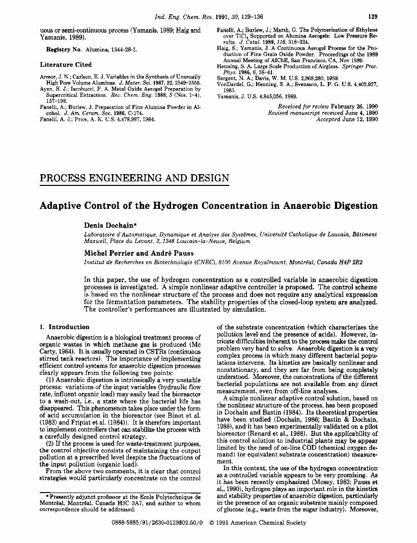
u Figure 1. Scheme of the anaerobic digestion.

hydrogen is easy to measure on-line (see Pauss et al., 1990). In this paper, a control algorithm of the hydrogen con-

centration is developed, which presents the following features: it is adaptive, in order to deal with the process parameter uncertainty; it is based on the nonlinear structure of the process; its theoretical stability and convergence properties are studied. In particular, its robustness with respect to neglected dynamics is analyzed by referring to singular perturbation arguments.

The paper is then organized as follows. Section 2 presents the dynamical model of anaerobic digestion including the hydrogen influence. Section 3 concentrates on the development and the theoretical properties of the control algorithm. The effectiveness of the adaptive controller is illustrated by different simulations in Section 4. In particular, its performances are compared to those of a fixed PI regulator.

2. Dynamical Model of Anaerobic Digestion The role of hydrogen in the kinetics of anaerobic di-

gestion has been recently emphasized by Mosey (1983). Four metabolic pathways can then be identified: two acidogenesis steps and two methanization steps (Figure 1).

In the first acidogenesis pathway (path l), glucose is decomposed into fatty volatile acids (acetate, propionate), hydrogen and inorganic carbon by acidogenic bacteria. In the second acidogenesis pathway (path 2), OHPA (obligate hydrogen-producing acetogens) decompose propionate into acetate, hydrogen, and inorganic carbon. In the first methanization pathway (path 3), acetate is transformed into methane and inorganic carbon by acetoclastic methanogenic bacteria, while in the second methanization pathway (path 4), hydrogen combines with inorganic carbon to produce methane under the action of hydrogenophilic methanogenic bacteria.

By using mass balance considerations in a CSTR, the following state space representation is readily obtained: path 1

(1) (2)

(3)

(4)

dXs/dt ~3x3 - DX3 (5) (6)

dXi/dt = pix1 - DX1 dS,/dt = -k lp iSI + DSi, - DS1

dXg/dt = ~2x2 - DX2 dS,/dt = -k2/~2X2 + k3~1X1- DS2

path 2

path 3

dS,/dt = - k 4 d 3 + k~,~iXi + k 8 ~ 2 X 2 - DS3

with

A =

0 3 k2k4k11 + kZkgk13 + k3k4k12 + k3k8k13

P 4 = klk4(k4k12 + k6k13)

P5 = klk2

@6 = P5k4

An important feature of the state variable z is that its dynamical equation is independent of the specific growth rates pi (i = 1-4). This allows us to emphasize the boundedness of the process variables independently of the usually badly known mathematical structure of the specific growth rates and under the following realistic assumptions:

(Al) The yield coefficients ki (i = 1-15) are positive and constant.

(A2) Xj(0) I 0 (i = 1-4), and Sj(0) L 0 0' = 1-5). (A3) D I 0 for all t I 0. (A4) 0 I Si, I S,,, and 0 I Shin 5 S5,= for all t L. 0. (A5) pi I 0 for all t I 0 (i = 149, pi(Si = 0) = 0 (i = 1-4),

and p4(S5) = 0.

Ind. Eng. Chem. Res., Vol. 30, No. 1, 1991 131

dynamics are faster than the corresponding acetate dynamics. Under this assumption, it is reasonable to believe that acting directly on the hydrogen concentration will prevent any process instability more quickly.

(3) The hydrogen concentration in the liquid phase is easier to measure on-line than any other substrate (COD, acetate, propionate) since it is basically a gas measurement (see Pauss et al. (1990)). It is assumed that the interphase hydrogen transfer is not limiting: the gas partial pressure thus reflects the hydrogen concentration in the liquid phase.

Statement of the Control Problem. Our objective is to control the hydrogen concentration S4 under the following conditions:

(Cl) The dilution rate D is the control input. (C2) The influent glucose concentration Si, and the

gaseous hydrogen flow rate Q1 are measured on-line. (C3) The specific growth rates pi (i = 1-4) are time-

varying and unknown. (C4) The yield coefficients are all unknown except k8/k l

(which is simply a yield coefficient between glucose and hydrogen).

Reformulation of the Dynamical Equations. Before deriving the adaptive control law, we shall first reformulate the dynamical model (1)-(10) for our control problem.

Let us consider the following assumptions: (A91 The propionate formation path is negligible; Le.,

Sz = X 2 = 0 and k3 = 0 in eqs 1-10. (A10) The acidogenic step kinetics (path 1) are much

faster than the dynamics of the methanogenic steps (paths 3 and 4).

The above assumptions appear to be in good accordance with the physical reality and the practical operation of anaerobic digestion reactors. Assumption A10 can be mathematically formalized by using singular perturbation arguments (Kokotovic et al., 1986; Lakin and Van den Driessche, 1977).

Let us consider an equilibrium point of the CSTR, and let us denote the equilibrium values of D, Xi, and SI as follows: D, Si, and Xi

If we define the following adimensional variables SI Si s i = - f = D t , e = - X i

= Z' SI' k l X 1

it is clear that the mass balance equations of the first acidogenesis path can be rewritten as follows

klk2k4S5max/P3. (A8) The specific growth rates p 3 and p4 are bounded:

pi I pi* (i = 3, 4). Theorem 1. Under assumptions Al-A8, the state vector

x and the methane gas flow rate Q3 are bounded as follows:

with

~ 0 0 0 0 0 0 0 0 1 1

Proof. Theorem 1 is a straightforward extension of lemma 1 in Dochain and Bastin (1984).

Comments. (1) Theorem 1 simply says that, with the above model (l)-(lO), the state variables, i.e., the reactant concentrations, will remain positive and bounded if the inputs D and Si, are positive and bounded (even without any upper bound on D being necessary): in that sense, it clearly strengthens the above model plausibility.

(2) We have mentioned in section 1 that one important feature of anaerobic digestion processes is their possibly unstable behavior. It is worth noting that the above BIBS stability result is compatible with the presence of (locally) unstable dynamical behavior: this instability can be represented theoretically (e.g. Dochain, 1986; Bastin and Dochain, 1990) and in simulation via the use, for instance, of an Haldane specific growth rate structure (as it will be illustrated in section 4). More precisely, in a simple mi- crobial growth process with one Haldane growth rate model, apart from the wash-out state, two different sets of equilibrium points can be associated to one value of the dilution rate D lower than the maximum value of the specific growth rate: one stable equilibrium point (corresponding to low substrate values) and one unstable equilibrium point (with higher substrate concentrations) (for further details on the properties of equilibrium points of stirred tank bioreactors, see Bastin and Dochain (1990)). In such an unstable equilibrium state, the process will be led in open loop to a wash-out by any disturbance. This requires a careful controller design in order to avoid this undesirable phenomenon.

(3) Assumption A5 (pi(Si=O) = 0) is simply the mathematical formulation of the (evident) feature that there is no growth without limiting substrate.

(4) Similarly, assumption A6 expresses that there is no hydrogen (respectively C02) gases flow rate without hydrogen (respectively inorganic carbon) in the liquid phase.

3. Adaptive Control of t he Hydrogen Concentration

In an automatic control context, the use of hydrogen as a controlled variable in anaerobic digestion appears to be very promising for the following three reasons:

(1) In some instances (e.g., in the presence of a glucose-type substrate (like wastewater from the sugar industry)), up to 30% of the methane gas may be produced from the hydrogen consumption.

(2) The two methanogenic pathways are, as far as we know, assumed to be essentially parallel, but the hydrogen

dxi 1.11 D _ - - -xi - -xi df D D

Note that t is defined as the ratio between the remaining glucose concentration that has not been consumed by the acidogenic reaction and the glucose concentration that has been transformed by the acidogenic bacteria (via a yield coefficient equal to k l ) . If we are considering the (realistic and often encountered in practice) situation when the steady-state of the process is characterized by a high glucose transformation (Le., a low value of Si and a high value of k l X 1 ) , then t is small:

si << k l X 1 * c << 1

The singular perturbation approximation consists of setting t = 0. Then we readily obtain the following alge- braic equation (which replaces the differential equation (2) or (12)):

~ I P ~ X I = Dsin (13)


Note that the above singular perturbation could have been directly obtained by setting S1 and its time derivative dS,/dt to zero in eq 2. The singular perturbation is simply the mathematical formalization of that model order re- duction often encountered in fermentation processes ap- plications. It is important to note that the singular approximation does not impose S1 to be equal to zero but simply to be small with respect to klXl. We shall see in theorem 2 how far from the ideal situation, when t = 0, the closed-loop system can theoretically go and yet remain stable.

Under assumptions A9 and A10, if we replace plX1 by its above expression (13), we can write the output dynamical equation (8) as follows:

dS,/dt = -DS4 + KDSi, - k 7 ~ 4 X 4 - Q1 (14)

with K = k8/kl. Let us now define

(1) the parameter (Y

P4 = as4 (15) (the above definition of the parameter a only implies, in accordance with the physical reality, that the hydrogenophilic methanogenic bacteria cannot grow in the absence of the limiting substrate S4 (i.e., p4 = 0 if S4 = 0)) (2) the auxiliary variable Z6

Z6 = KSI + S4 + k7X4 (16)

Z6 = S4 + k7X4 if t = 0 (17) Under assumption A9, Z6 has the following dynamical behavior:

(18)

By using the above definition, we can rewrite the output dynamical equation (14):

dS4/dt = -DS4 + KDSi, - aS4(Z6 - S4) - Q1 (19)

The derivation of the control algorithm is based on the above output dynamical equation (19).

dz,/dt = -DZ6 + KDSi, - Q1

The Control Algorithm. Define the control error s4 = s4* - s4 (20)

Consider that we wish to have the following first-order where S4* is the desired hydrogen concentration.

linear closed-loop dynamics: dS,/dt + CIS4 = 0 C1 > 0 (21)

The above closed-loop dynamics will be achieved by implementing the following nonlinear control law:

CIS4 + dS4*/dt + aS4(Z6 - S4) + Q1 D = (22) KSi, - S4

Since CY is unknown and Z6 is not a measured variable, we consider an adaptive version of the nonlinear control law (22):

Cis4 + dS,*/dt + aS4(& - 5'4) + Q1 KSi, - S4 D = (23)

where Z6 is estimated by using eq 18; i.e., d i6 /d t = -DZs + KDSi, - Q, (24)

and & is updated as follows

cz > 0 (25)

i.e., by using here a Lyapunov design estimation algorithm

I

ESTIMATION

0 - b I A , I I

I 1 I " ' I

Figure 2. Schematic view of the adaptive controller.

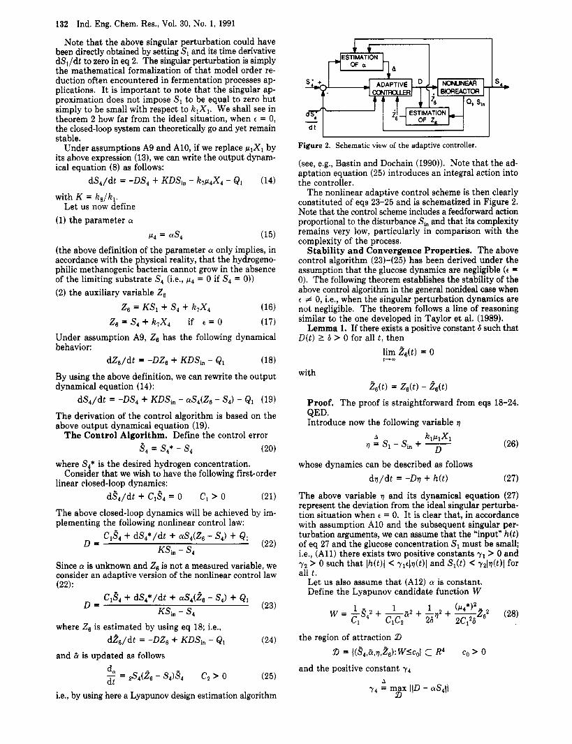
(see, e.g., Bastin and Dochain (1990)). Note that the ad- aptation equation (25) introduces an integral action into the controller.

The nonlinear adaptive control scheme is then clearly constituted of eqs 23-25 and is schematized in Figure 2. Note that the control scheme includes a feedforward action proportional to the disturbance Si, and that its complexity remains very low, particularly in comparison with the complexity of the process.

Stability and Convergence Properties. The above control algorithm (231425) has been derived under the assumption that the glucose dynamics are negligible (t = 0). The following theorem establishes the stability of the above control algorithm in the general nonideal case when t # 0, i.e., when the singular perturbation dynamics are not negligible. The theorem follows a line of reasoning similar to the one developed in Taylor et al. (1989).

Lemma 1. If there exists a positive constant 6 such that D ( t ) I 6 > 0 for all t , then

lim 26(t) = o t--

with 26(t) = Z6(t) - 26(t)

Proof. The proof is straightforward QED. Introduce now the following variable

A klP1Xl q = s, - si, + 7

from eqs 18-24.

D

(26)

whose dynamics can be described as follows dq/dt = -Dq + h(t) (27)

The above variable q and its dynamical equation (27) represent the deviation from the ideal singular perturbation situation when e = 0. It is clear that, in accordance with assumption A10 and the subsequent singular perturbation arguments, we can assume that the "input" h(t) of eq 27 and the glucose concentration S1 must be small; Le., (Al l ) there exists two positive constants y1 > 0 and y2 > 0 such that Ih(t)l C yltlq(t)l and Sl(t) r2lq(t)l for all t .

Let us also assume that (A12) a is constant. Define the Lyapunov candidate function W

1 - 1 1 (P4*)2 - C1 c,c2 26 2C126

W = -S4* + -it2 + -q2 + -26' (28)

the region of attraction D

and the positive constant y4 A

y4 = max {ID - aS411 a,


Then we can deduce the following stability result. Theorem 2. Under assumptions A1-A12, if co is such

that D ( t ) 2 6 > ?for all t and C, > K ( y 2 y 4 + y4 + p4*) A y3, then for all (S4(0),n(O),~(O),Z~(0)) E 52 and for every 6 satisfying

23 is a region of attraction for s4(5), C ( t ) , ? ( t ) , and &(t) for all t 2 0, and

lim S 4 ( t ) = o lim ? ( t ) = o t-- t--

Proof. After some straightforward calculations, it can be shown that the time derivative of W is bounded as follows:

d W / d t I ETQ[

Y3 -1 -

Q = [ 2 c1 -1 + - €;'I By definition of t, d W / d t is therefore negative definite in 5, and the rest of the proof follows from Lasalle's theorem (1968) and a result from Peiffer and Rouche (1969).

QED. Comments. (1) The above theorem shows that, as far

as C1 > y3, the closed-loop system remains stable for sufficiently small value of 6, i.e., if assumption A10 is fulfilled.

(2) In order to prove the above theorem, we had to introduce a positive condition on the dilution rate D ( D ( t ) 2 6 > 0). In practice, D has to be obviously positive: ideally, such a condition should appear explicitly in the control. However, the stability analysis would then be much more involved (as illustrated on a similar but simpler case in Dochain (1986)).

4. Simulation Results The performances of the nonlinear adaptive controller

have been tested by performing extensive simulation experiments. Simulation of the anaerobic digestion process has been carried out by integrating eqs 1-8 with the following set of yield coefficient values and specific growth rate expressions (which are obviously completely ignored by the adaptive controller):

kl = 3.2, k2 = 1.5, k, = 0.7, k4 = 16.7, k, = 0.27, k6 0.53, k7 = 1.15, k8 = 0.6, kg = 0.1

pl = a1S1 with a1 = 0.2 L/(g day) (Blackman model)

with p2*= 0.5 day-' and KM2 = p2*s2

" = KM2 + S2 0.4 g/L (Monod model)

for i = PiOSi

KMi + Si + S:/KIi Pi =

3, 4 (Haldane model)

with p: = 0.3 day-', KM3 = 4 g/L, K13 = 21 g/L, p40 = 0.5 day-', K M 4 = 4 pM, K14 = 3 pM.

Note that the Haldane models have been chosen to characterize the two methanogenic paths (paths 3 and 4)

: closed loop (adaptive control) : open loop (constant D)

____-__----__-. ,o 40 80 120

Y S4=3pM

40 80 120

time (d) 0 -

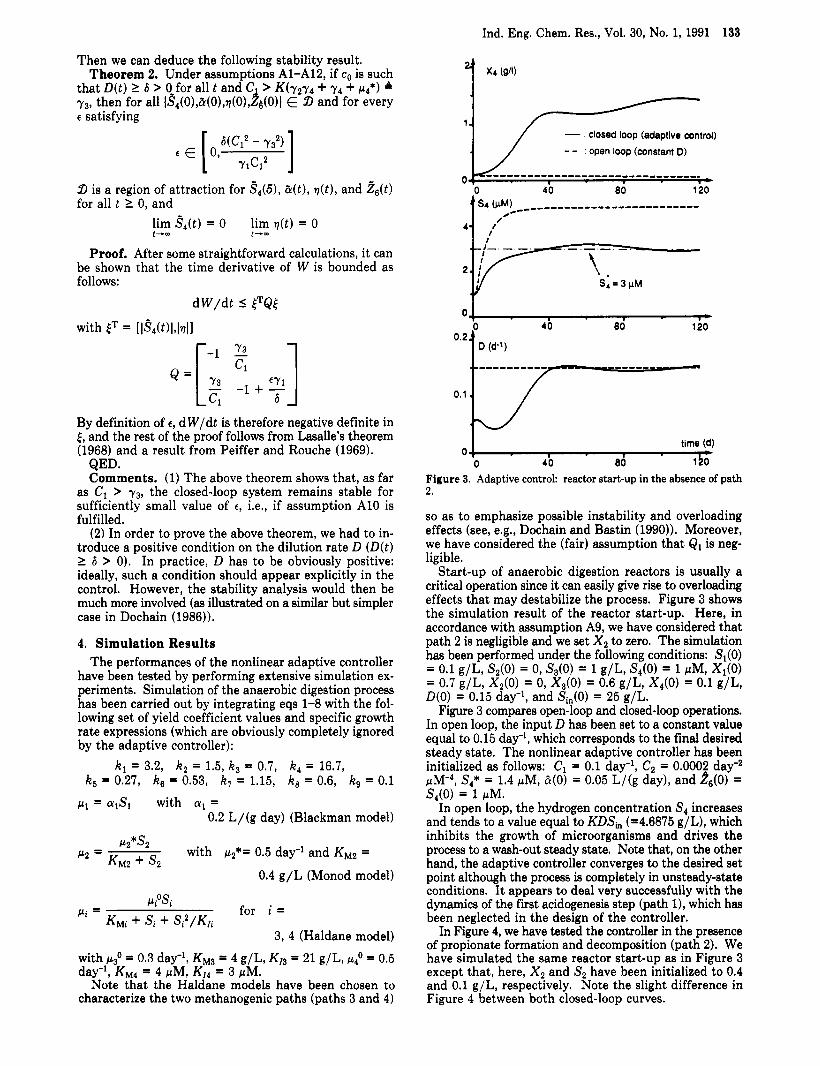
Figure 3. Adaptive control: reactor start-up in the absence of path 0 40 80 1 bo

n L.

so as to emphasize possible instability and overloading effects (see, e.g., Dochain and Bastin (1990)). Moreover, we have considered the (fair) assumption that Q1 is negligible.

Start-up of anaerobic digestion reactors is usually a critical operation since it can easily give rise to overloading effects that may destabilize the process. Figure 3 shows the simulation result of the reactor start-up. Here, in accordance with assumption A9, we have considered that path 2 is negligible and we set X 2 to zero. The simulation has been performed under the following conditions: Sl(0) = 0.1 g/L, S,(O) = 0, S3(0) = 1 g/L, S4(0) = 1 pM, Xl(0) = 0.7 g/L, X2(0) = 0, X&O) = 0.6 g/L, X4(0) = 0.1 g/L, D(0) = 0.15 day-', and Si,(0) = 25 g/L.

Figure 3 compares open-loop and closed-loop operations. In open loop, the input D has been set to a constant value equal to 0.15 day-', which corresponds to the final desired steady state. The nonlinear adaptive controller has been initialized as follows: C1 = 0.1 day-', C2 = O.OOO? day-, PM-~, S4* = 1.4 pM, N O ) = 0.05 L/(g day), and Z6(0) = S4(0) = 1 pM.

In open loop, the hydrogen concentration S4 increases and tends to a value equal to KDSh (=4.6875 g/L), which inhibits the growth of microorganisms and drives the process to a wash-out steady state. Note that, on the other hand, the adaptive controller converges to the desired set point although the process is completely in unsteady-state conditions. I t appears to deal very successfully with the dynamics of the first acidogenesis step (path l), which has been neglected in the design of the controller.

In Figure 4, we have tested the controller in the presence of propionate formation and decomposition (path 2). We have simulated the same reactor start-up as in Figure 3 except that, here, X 2 and S2 have been initialized to 0.4 and 0.1 g/L, respectively. Note the slight difference in Figure 4 between both closed-loop curves.


1.'

'1 / _ _ : Path 2 is neglected

I *

- : with Path 2 (OHPA-proprionate)

O . 7 D (d-l)

time (d) I 1 -

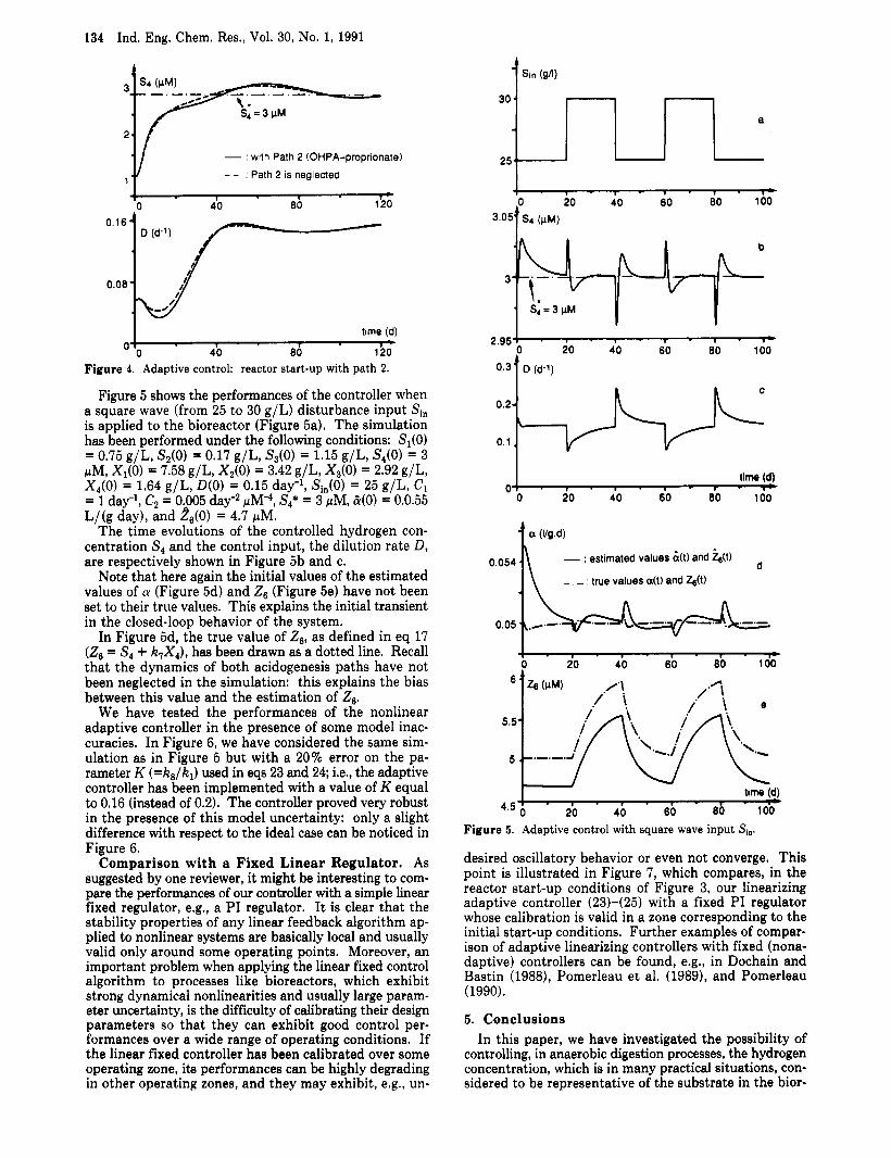
40 80 120 Figure 4. Adaptive control: reactor start-up with path 2.

Figure 5 shows the performances of the controller when a square wave (from 25 to 30 g/L) disturbance input Si, is applied to the bioreactor (Figure 5a). The simulation has been performed under the following conditions: Sl(0) = 0.75 g/L, S,(O) = 0.17 g/L, S3(0) = 1.15 g/L, S4(0) = 3 pM, Xl(0) = 7.58 g/L, X,(O) = 3.42 g/L, X3(0) = 2.92 g/L, X4(0) = 1.64 g/L, D(0) = 0.15 dag1, Si,(0) = 25 g/L, C1 = 1 day-', C2 = 0,005 day-, pM4, S4* = 3 pM, &(O) = 0.0.55 L/(g day), and ZJO) = 4.7 pM.

The time evolutions of the controlled hydrogen concentration S4 and the control input, the dilution rate D, are respectively shown in Figure 5b and c.

Note that here again the initial values of the estimated values of (Y (Figure 5d) and Z6 (Figure 5e) have not been set to their true values. This explains the initial transient in the closed-loop behavior of the system.

In Figure 5d, the true value of Z6, as defined in eq 17 (Z6 = S4 + k7X4) , has been drawn as a dotted line. Recall that the dynamics of both acidogenesis paths have not been neglected in the simulation: this explains the bias between this value and the estimation of Zg.

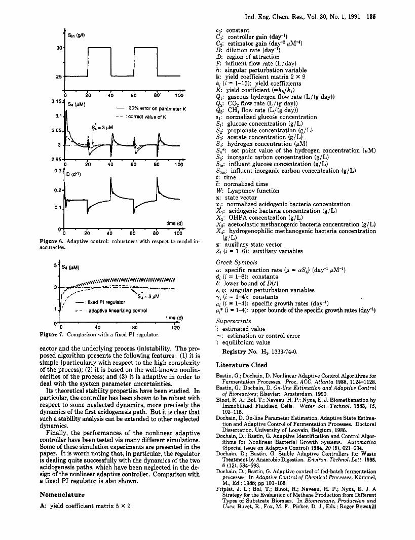
We have tested the performances of the nonlinear adaptive controller in the presence of some model inac- curacies. In Figure 6, we have considered the same simulation as in Figure 5 but with a 20% error on the parameter K ( = k 8 / k l ) used in eqs 23 and 24; Le., the adaptive controller has been implemented with a value of K equal to 0.16 (instead of 0.2). The controller proved very robust in the presence of this model uncertainty: only a slight difference with respect to the ideal case can be noticed in Figure 6.

Comparison with a Fixed Linear Regulator. As suggested by one reviewer, it might be interesting to com- pare the performances of our controller with a simple linear fixed regulator, e.g., a PI regulator. I t is clear that the stability properties of any linear feedback algorithm applied to nonlinear systems are basically local and usually valid only around some operating points. Moreover, an important problem when applying the linear fixed control algorithm to processes like bioreactors, which exhibit strong dynamical nonlinearities and usually large parameter uncertainty, is the difficulty of calibrating their design parameters so that they can exhibit good control performances over a wide range of operating conditions. If the linear fixed controller has been calibrated over some operating zone, its performances can be highly degrading in other operating zones, and they may exhibit, e.g., un-

Sin 1

I time (d) . .- i o . i o ' $0 . i o 100

u r - 0

' a (11g.d)

d - : estimated values &(t) and Z&t)

- - : true values a(t) and &(t)

I , . . . , . , . . - + ? 20 40 60 80 100

Figure 5. Adaptive control with square wave input Si,.

desired oscillatory behavior or even not converge. This point is illustrated in Figure 7, which compares, in the reactor start-up conditions of Figure 3, our linearizing adaptive controller (23)-(25) with a fixed PI regulator whose calibration is valid in a zone corresponding to the initial start-up conditions. Further examples of comparison of adaptive linearizing controllers with fixed (nona- daptive) controllers can be found, e.g., in Dochain and Bastin (1988), Pomerleau et al. (1989), and Pomerleau (1990).

5. Conclusions In this paper, we have investigated the possibility of

controlling, in anaerobic digestion processes, the hydrogen concentration, which is in many practical situations, considered to be representative of the substrate in the bior-


80 100 0 20 40 60

- : 20% error on parameter K - - : correct value of K 3.1

3 . 0 5 1 1 3 8 0

2.954 . , . , . , . , . , 0 20 40 60 80 100

time (d)

20 40 60 80 100

Figure 6. Adaptive control: robustness with respect to model in- accuracies.

s d (W

: fixed PI regulator : adaptive linearizing control

time (d) I f

O'0 40 80 120 Figure 7. Comparison with a fixed PI regulator.

eactor and the underlying process (in)stability. The proposed algorithm presents the following features: (1) it is simple (particularly with respect to the high complexity of the process); (2) it is based on the well-known nonlinearities of the process; and (3) it is adaptive in order to deal with the system parameter uncertainties.

Its theoretical stability properties have been studied. In particular, the controller has been shown to be robust with respect to some neglected dynamics, more precisely the dynamics of the first acidogenesis path. But it is clear that such a stability analysis can be extended to other neglected dynamics.

Finally, the performances of the nonlinear adaptive controller have been tested via many different simulations. Some of these simulation experiments are presented in the paper. It is worth noting that, in particular, the regulator is dealing quite successfully with the dynamics of the two acidogenesis paths, which have been neglected in the design of the nonlinear adaptive controller. Comparison with a fixed PI regulator is also shown.

Nomenclature A: yield coefficient matrix 5 x 9

c,,: constant C1: controller gain (day-') C,: estimator gain (day-2 P M - ~ ) D: dilution rate (day-') a: region of attraction F influent flow rate (L/day) h: singular perturbation variable k: yield coefficient matrix 2 x 9 ki (i = 1-15): yield coefficients K: yield coefficient ( = k , / k , ) Q1: gaseous hydrogen flow rate (L/(g day)) Q,: COz flow rate (L/(g day)) Q3: CH, flow rate (L/(g day)) sl: normalized glucose concentration S1: glucose concentration (g/L) S,: propionate concentration (g/L) SB: acetate concentration (g/L) S4: hydrogen concentration (pM) S4*: set point value of the hydrogen concentration (pM) S5: inorganic carbon concentration (g/L) Sin: influent glucose concentration (g/L) SSin: influent inorganic carbon concentration (g/L) t : time f: normalized time W Lyapunov function x: state vector xl: normalized acidogenic bacteria concentration X1: acidogenic bacteria concentration (g/L) X,: OHPA concentration (g/L) X 3 : acetoclastic methanogenic bacteria concentration (g/L) X4: hydrogenophilic methanogenic bacteria concentration

z: auxiliary state vector Zi (i = 1-6): auxiliary variables

Greek Symbols a: specific reaction rate ( p = as4) (day-' pM-l) pi (i = 1-6): constants 6: lower bound of D(t ) t, 7: singular perturbation variables y i (t = 1-4): constants pi ( I = 1-4): specific growth rates (day-') pi* (i = 1-4): upper bounds of the specific growth rates (day-') Superscr ip ts *: estimated value -: estimation or control error -: equilibrium value

Registry No. H,, 1333-74-0.

(g/L)

Literature Cited Bastin, G.; Dochain, D. Nonlinear Adaptive Control Algorithms for

Fermentation Processes. Proc. ACC, Atlanta 1988, 1124-1128. Bastin, G.; Dochain, D. On-line Estimation and Adaptioe Control

of Rioreactors; Elsevier: Amsterdam, 1990. Binot, R. A.; Bol, T.; Naveau, H. P.; Nyns, E. J. Biomethanation by

Immobilized Fluidised Cells. Water Sci. Technol. 1983, 15,

Dochain, D. On-line Parameter Estimation, Adaptive State Estima- tion and Adaptive Control of Fermentation Processes. Doctoral Dissertation, University of Louvain, Belgium, 1986.

Dochain, D.; Bastin, G. Adaptive Identification and Control Algor- ithms for Nonlinear Bacterial Growth Systems. Automatica (Special Issue on Adaptive Control) 1984, 20 ( 5 ) , 621-634.

Dochain, D.; Bastin, G. Stable Adaptive Controllers for Waste Treatment by Anaerobic Digestion. Enuiron. Technol. Lett. 1981,

Dochain, D.; Bastin, G. Adaptive control of fed-batch fermentation Drocesses. In AdaDtiue Control of Chemical Processes: Kummel.

103-115.

6 (12), 584-593.

M., Ed.; 1988; pp'lO3-108. FriDiat. J. L.: Bol. T.: Binot. R.: Naveau. H. P.: Nvns. E. J. A

Strategy for the Evaluation i f Methane Production fiom'Different Types of Substrate Biomass. In Biomethane, Production and Uses; Buvet, R., Fox, M. F., Picker, D. J., Eds.; Roger Bowskill

136 Ind. Eng. Chem. Res . 1991, 30, 136-141

Ltd.: Exeter, U.K., 1984; pp 95-105. Lakin, W. D.; Van den Driessche, P. Time scales in population bi-

ology. SIAM J. Appl. Math. 1977,32,694-705. Lasalle, J. P. Stability Theory for Ordinary Differential Equations.

J . Differ. Equations 1968, 4 , 57-65. Mc Carty, P. L. Anaerobic Waste Treatment Fundamentals. Public

Works 1964, Sept, 107-112; Oct, 123-126; Nov, 91-94; Dec, 95-99. Mosey, F. E. Mathematical Modelling of the Anaerobic Digestion

Process: Regulatory Mechanisms for the Formation of Short- chain Volatile Acids from Glucose. Water Sci. Techno!. 1983,15,

Pauss, A.; Beauchemin, C.; Samson, R.; Guiot, S. Continuous Mea- surement of Dissolved H2 in Anaerobic Digestion Using a Com- mercial Probe Hydrogen/Air Fuel Cell-based. Biotechno!. Bioeng.

Peiffer, K.; Rouche, N. Liapunov’s Second Method Applied to Par-

209- 23 2.

1990, 35, 491-502.

tial Stability. J . MBc. 1969, 8 (2), 323-334.

Pomerleau, Y. Mod6lisation et contrBle d’un procBdB fed-batch de cultures des levures ti pain. Ph.D. Thesis, Ecole Polytechnique de MontrBal, Canada, 1990.

Pomerleau, Y.; Perrier, M.; Dochain, D. Adaptive nonlinear control of the Baker’s yeast fed-batch fermentation. Proc. 1989 Am. Control Conf. (Invited Session on Intelligent Systems and Ad- vanced Control Strategies in Biotechnology), 1989,2,2424-2429.

Renard, P.; Dochain, D.; Bastin, G.; Naveau, H. P.; Nyns, E. J. Adaptive Control of Anaerobic Digestion Processes. A Pilot-scale Application. Biotechno!. Bioeng. 1988, 31, 287-294.

Taylor, D. G.; Kokotovic, P. V.; Marino, R.; Kanellapoulos, I. Adaptive Regulation of Nonlinear Systems with Unmodelled Dy- namics. IEEE Trans. Autom. Control 1989, 405-412.

Received for review February 2, 1990 Revised manuscript received July 2, 1990

Accepted July 24, 1990

A General Equation for the Heat-Transfer Coefficient at Wall Surfaces of Gas/Solid Contactors

Daizo Kunii Fukui Institute of Technology, 3-6-1 Gakuen, Fukui City, 910 Japan

Octave Levenspiel* Chemical Engineering Department, Oregon Sta te University, Coruallis, Oregon 97331 -2702

The general equation derived here accounts for the thermal properties of the solids, the particle size, the properties of the gas, the state of the gas/solid system (bubbling characteristics), and the contribution of radiation transfer. This equation reduces to a variety of simpler special case expressions: for fine particle and for large particle fluidized beds, for low-temperature operations, a t the surfaces immersed in both fluidized and moving beds, and for the tube wall surfaces of fast fluidized beds. All these expressions are simple to use, and we point out where these expressions have been tested against the reported experimental data.

The study of heat interchange between surfaces and fluidized beds has a long history, and numerous expressions have been proposed to represent the heat-transfer coefficient in this situation. Reviews of these studies can be found in Gelperin and Einstein (I), Botterill (2), Xavier and Davidson (3), and Baskakov ( 4 ) .

In this paper, we propose to develop a general equation for h to encompass a broad spectrum of conditions and operations. I t reduces to a number of special cases for various contacting regimes, including the freeboard, moving bed, and fast fluidization regimes.

Development of the General Equation We start by considering heat transfer in fixed and in-

cipiently fluidized beds and then extend this analysis to bubbling fluidized beds, to the freeboard region, and to fast fluidized beds.

Within a Fixed Bed with Stagnant Gas. If heat flows in parallel paths through the gas and the solid, then the effective thermal conductivity of the fixed bed would be given by

(1) k: = tm$g + (1 - emf)ks

Here, the superscript ‘‘0” refers to stagnant gas conditions, and 4b = d,,,/d, represents the equivalent thickness of stagnant gas film around the contact points between particles, which aids in the transport of heat from particle to particle. Since 4b depends on the bed voidage and since we are interested in using eq 2 later in our fluidized bed development, Figure 1 gives the values of 4b for the loosest packing of a normal fixed bed, which is at about = 0.476.

For most gas/solid systems, k, >> k,; thus, the last part of the second term in eq 2 is smaller than unity. This means that the thermal conductivity of a fixed bed is lower than for the parallel path model of eq 1.

At the Wall of a Fixed Bed with Stagnant Gas. Consider the wall region to extend a half particle diameter out from the heat-exchange surface. Then, similar to eq 2, the thermal conductivity in this layer can be represented by

However, to account for the actual geometry and the small Contact region between adjacent particles, Kunii and Smith (5) developed the following modification to the parallel path model:

where e, is the mean void fraction of this wall layer. Kunii and Suzuki (6) derived the above equation and used it successfully to represent the surface heat-transfer data reported by workers at that time. They also explained why a thickness of half a particle diameter was selected to represent the wall region.

Figure 1 shows the calculated values for 4,, defined as the equivalent thickness of stagnant film at a contact point between a sphere and the wall surface. Note that the

r 1 (2)

0888-5885/91/2630-0136$02.50/0 0 1991 American Chemical Society

adaptive control of the hydrogen concentration in anaerobic digestion

Documents