adaptive and robust query processing with sharp

University of Wisconsin – Madison, Computer Sciences Department Technical Report #1562, April 2006

Adaptive and Robust Query Processing with SHARP

Pedro Bizarro David J. DeWitt

University of Wisconsin – Madison University of Wisconsin – Madison

[email protected] [email protected]

Abstract Database catalogs often do not contain enough statistical information to correctly cost all possible physi-cal plans. In their absence, the optimizer can produce incorrect estimates and select sub-optimal plans for execution. To address this problem for a sub-class of queries, we propose SHARP, a new multi-join, adaptive, relational operator that joins three or more relations of a star-join. SHARP reduces the possible impact of optimizer mistakes by determining which plan to execute independently of optimization esti-mates. During normal query processing, SHARP collects statistics, and by using a combination of late-binding plan decisions and tuple routing strategies, it is able to change join order and table access meth-ods. However, unlike previous tuple routing operators used for in-memory stream processing, SHARP was designed to process local relations with sizes much larger than available memory. We have imple-mented SHARP in the open-source DBMS Predator, and we present an extensive experimental evalua-tion showing the significant performance benefits of SHARP.

1. INTRODUCTION Database optimizers cost and choose query plans as if they have precise information about data distribu-tions. However, that is rarely the case. When statistics are not available in the catalog, the optimizer es-timates them by assuming that some data distributions are uniform or independent, by using a combination of other (possibly estimated) statistics, or even by using default values [37]. These esti-mates may contain errors that grow exponentially with the number of estimated statistics derived from other estimated statistics [23] and the chosen plans may be sub-optimal by orders of magnitude [32]. Having more information in the catalog (e.g., histograms [34]) reduces the problem, but the information needed to correctly cost all possible query plans is likely to increase exponentially as database sizes grow, as queries become larger, and as query languages become more complex. If that is the case, then database optimizers may have insufficient information to choose good, non-adaptive query plans for all queries. Instead, decisions about which query plan to run may have to be made at run-time–using adap-tive operators and/or late binding decisions–after some of the data is observed.

Following this reasoning, we propose SHARP1, a new, adaptive, relational operator for processing star-joins with three or more relations. At run-time, after observing some data, SHARP can opportunistically choose any possible join order to process those relations (without using Cartesian products). These plan changes are made using a combination of late-binding plan decisions and tuple routing strategies. In ad-dition, although tuple routing has previously been used mainly for in-memory data processing, SHARP does not keep all the joins completely in memory. This allows SHARP to have both a smaller memory

1 Streaming, Highly Adaptive, Run-time Planner


footprint than other adaptive operators [16, 44], and to have an efficient second pass to process relations much larger than available memory.

1.1 Contributions and Outline of the Paper The main contributions of this paper are the following:

•••• In Section 3.1, we introduce SHARP, a new, multi-join, adaptive, operator to process star-joins.

•••• We show that tuple routing policies used in data stream systems can be used in traditional databases processing relations larger than memory. We also provide the first apples-to-apples comparison of three tuple routing policies [2, 5, 15] in the same system. These policies are described in Section 3.2.

•••• We propose a series of late-binding decisions that can opportunistically change the query plan at run-time to improve performance. These decisions, described in Section 3.3, are taken after SHARP has seen some tuples, but before deciding on the final execution plan.

•••• We propose a new multi-join second-stage processing algorithm in Section 3.4. This algorithm shows good improvements over alternative techniques and its performance is insensitive to optimizer mis-takes.

•••• As described in Section 4, we implement and evaluate a prototype implementation of SHARP in Predator [38]. The results show good performance improvements over plans not using SHARP.

2. EDDIES AND MJOINS The operators most related to SHARP are the Eddy [2] and the MJoin [44], both multi-join adaptive op-erators using tuple routing. They are described here to provide context for the SHARP contributions in the next Section. Other related work appears in Section 5.

2.1 Terminology For an operator Op joining two or more relations, we say relation B is a build relation when tuples from that relation are inserted into some lookup structure (e.g., hash tables). We say relation D drives Op, or is a driving (or probing) relation for Op, if each input tuple t1 coming from D probes the build lookup structures of Op and potentially produces output tuples, or schedules t1 for second-stage processing, be-fore any other tuple t2 from D is processed2. A relation may be simultaneously a build and driving rela-tion. In the figures, driving relations are marked with arrowed lines and build relations are marked with dotted lines.

2.2 The Eddy The Eddy [2] is an operator that routes tuples through a pool of operators until they are processed by all operators or are dropped along the way. The Eddy continuously observes the performance of the opera-tors by collecting statistics at run-time (e.g., selectivity and cost) and routes tuples to the most efficient operator3. Since these statistics are potentially changing, the process is automatically adaptive, possibly sending different tuples through different routes. The ability to efficiently change routes (i.e., query plans) relies on operators with moments of symmetry [2], moments after which joins can be reordered. The symmetric hash join (SHJ) [45], typically used with Eddies, is an operator with frequent moments

2 For example, in a nested-loops join operator the left input is the driving source, and in a hybrid hash join operator the right

input is the driving source. 3 In reality, the Eddy routes most, but not all, tuples through the route expected to be most efficient (in a process called ex-

ploitation) and simultaneously routes some few tuples through other routes to discover if any of those other routes has be-come the most efficient (exploration).


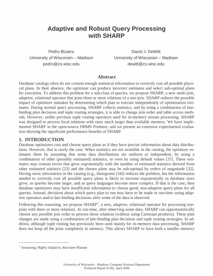
of symmetry. Each SHJ consists of two in-memory hash tables4, one for each relation being joined; tu-ples from one relation build into its hash table and probe the other. An Eddy with SHJs can then execute several plans, depending on the tuple source and routing policy. For example, the Eddy in Figure 1b executes R aS bT by sending R tuples to first probe hash table S.a and then probe T.b, T tuples first probe S.b and then R.a, and S tuples have two options: either they first probe T.b and then R.a, or first they probe R.a and then T.b (hash tables are represented as grey rectangles in Figure 1). This design, al-beit providing very adaptive plans, introduces a considerable overhead [15]: it requires maintaining two hash tables per join and requires that all joins be completely and simultaneously in memory (e.g., the Eddy of Figure 1b needs to maintain the four hash tables, R.a, S.a, S.b, and T.b in memory). Although the Eddy has the potential to join any number of relations in any order, its memory limitations restrict the Eddy for in-memory processing of data streams (possibly infinite, window-bounded, remote tuple sources that deliver tuples at unpredictable and bursty rates).

2.3 The MJoin The MJoin [44] is a completely symmetric multi-way data stream join operator, with one hash table per data stream. As with the Eddy using SHJs, tuples from a particular source build on that source’s hash table and probe the others. The MJoin uses fewer hash tables than the Eddy because it assumes that a data stream uses the same joining attribute for the all joins (see Figure 1c). This assumption also allows more join orders in the MJoin than in the Eddy. For example, the MJoin of Figure 1b can process any of the six join orders (RST, RTS, SRT, STR, TRS, and TSR), being restricted only by the incoming tuple source.

The important contributions of MJoins are i) producing tuples sooner than a tree of binary non-blocking join operators (e.g., SHJs), ii) extending the streaming behavior of SHJs to allow memory overflow, and iii) providing a rate-based cost model of the data stream join problem it addresses.

In contrast, our paper addresses the problem of joining local relations. Our goal is to execute plans that are insensitive to optimizer mistakes and our evaluation metric is time to completion. Other differences between the MJoin and SHARP are: the MJoin does not redistribute memory dynamically between joins, requires more memory then SHARP, does not evaluate routing policies, and, for the second-pass, assumes that all relations join on the same attribute.

4 Each one of the two hash-tables that composes a SHJ is called a SteM in the Eddies nomenclature [35].

S

Figure 1 – A SHARP and an Eddy processing R aS bT, and a MJoin processing R aS aT.

Eddy

R aS R.a S.a

R S T

S bT S.b T.b

R.a

R T

Output Output

R.a S.a

R S T

T.a

Output

T.b

a) SHARP c) MJoin b) Eddy

SHARP

MJoin


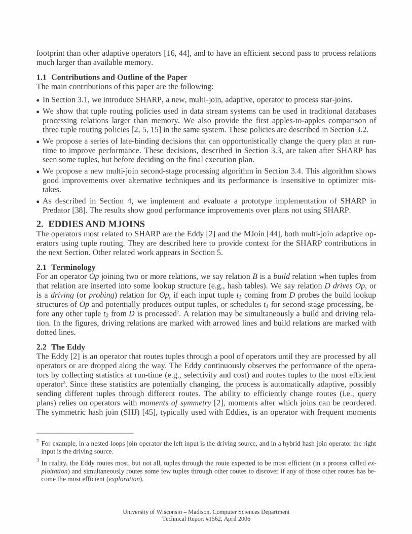
3. SHARP SHARP is an operator that keeps the inexpensive [15], tuple-routing, run-time adaptivity of the Eddy without incurring the overhead of SHJs [15] and without the requirement that all joins fit completely in memory. The trade-off is that, while Eddies and MJoins can process arbitrary plans, SHARP processes only star-joins and segments of linear-joins as shown in Figure 2. In spite of that, SHARP still has the potential to adaptively decide at run-time which join order to use. In addition to reducing memory usage, not using SHJs also allowed the development of a new technique to process joins between relations much larger than memory.

The rest of this Section is organized as follows. Section 3.1 describes the in-memory behavior of SHARP and minor multi-join improvements. Section 3.2 describes three tuple routing techniques im-plemented in SHARP. Section 3.3 introduces late-binding decisions that allow SHARP to change the query plan before tuple routing starts. Then, Section 3.4 describes how SHARP processes relations lar-ger than memory. Finally, Section 3.5 summarizes SHARP and compares it with Eddies and MJoins.

3.1 In-Memory Processing In a SHARP joining n relations, one relation is the single driving relation and all other n-1 relations are build relations. SHARP starts by reading tuples from the build relations and creates an in-memory hash table for each one. (Processing of build relations bigger than available memory is described in Section 3.4) Then, SHARP reads tuples from the driving relation, probes the in-memory build hash tables and outputs join results. Figure 1 (previous page) shows a SHARP joining R aS bT, where R and T are the build relations and S is the driving relation. Tuples from the driving relation–henceforth called driving tuples–probe the build hash tables in an order specified by an adaptive tuple routing policy, as described in Section 3.2.

3.1.1 Adaptive Redistribution of Memory. In SHARP, each build hash table is given a memory budget. If the total build size is larger than the budgeted amount, then the hash table must write hash partitions to disk for second-stage processing. However, before writing them to disk, SHARP first loads the remaining build tables into memory until they either consume their entire memory budget or load completely. If any budget is underutilized, SHARP reassigns the available memory to the yet to finish build hash tables. In contrast, the process of redistributing memory across joins is non-trivial for tree-shaped execution plans of binary operators. The process is more difficult because operators lower in the tree cannot obtain excess memory from opera-tors higher in the tree as they have not begun execution.

Note that many memory redistribution policies are possible. For simplicity, SHARP assigns all unused build memory to the first hash table build that did not fit its budget. If that build completes without using

Figure 2 – A SHARP processing a star-join, and two SHARPs processing a linear-join

A

Star-Join

E C

B

D

D C B A E

SHARP

A

Linear-Join

B C

C B C

D E

E A

SHARP

SHARP


all the newly assigned extra memory, SHARP further reassigns it to the next yet to finish build and so on.

3.1.2 Multi-Join Optimizations. SHARP takes advantage of its multi-join nature to obtain two performance benefits. First, SHARP avoids creating some intermediate results: when a tuple s from driving relation S, probes build relation R and finds a matching tuple r, the resulting rs is not generated. Instead, SHARP (like the Eddy’s imple-mentation in TelegraphCQ [11]) merely keeps a pointer to r and proceeds to probe the other build rela-tion T using tuple s. Then, an rst intermediate tuple is generated only if a matching tuple t of T is found. If the probe on T fails, no intermediate tuple is ever generated.

Another benefit is the reduction of getNext calls. Assume operator Op1 sends an s tuple to probe build hash table R and gets one single matching tuple r. In this scenario, two getNext calls are made on R: the first call returns r and the second call returns null, meaning that there are no more matches for s. In a traditional plan composed of binary hash join operators, the intermediate join tuple s.r is returned to Op2, the parent of Op1, before the second call is made. Op2 may then use the s portion of s.r to probe an-other hash table T. If the s.r probe on T fails, Op2 tries to get a new tuple from Op1. Op1 then finishes the probe of s on R by executing the second getNext call. This call is unnecessary: even if there was another tuple in R, say r2, matching with s, the s.r2 tuple would also be dropped by Op2 since it shares the same s component that failed the T probe. With SHARP, if a driving tuple probe into a build hash table returns no matches, then any outstanding open probes on other build hash tables are closed and spurious getNext calls are not made.

These two factors explain why SHARP shows a small performance advantage over trees of binary op-erators, even in scenarios where its adaptive mechanisms provide no benefit.

3.2 Adaptive Tuple Routing Strategies Used In SHARP, we implemented three routing policies adapted from three previous proposals [2, 15, 5].

The first routing policy, which we call Continuous or simply Cont, is a modification on the original rout-ing policy in the first Eddies paper [2]: a probabilistic routing mechanism based on lottery scheduling is used to determine where to route tuples next and routing decisions happen each time an operator finishes processing one tuple. The variation is that in Cont, we make a routing plan once per each driving tuple, instead of once per probe. In addition, instead of lottery scheduling, we route every r-th tuple to a ran-dom route. This makes the exploration mechanism independent of the currently estimated best route. For all other tuples Cont uses the estimated best routing order. Also, as in the Eddies implementation in TelegraphCQ [11], the selectivity of operators (the join selectivity of build hash tables in our case) is continuously updated after each probe and dropped tuples do not affect the selectivity of operators they do not probe.

Continuous-Batch, or simply ContB, the second tuple routing policy implemented, is taken from Deshpande [15]: instead of computing a routing order once per driving tuple, routing orders are com-puted once per batches of tuples. Policies Cont and ContB minimize the overhead of gathering statistics–tuples are not used to explore operators after being dropped–but they provide no optimality guarantees on the chosen routes: they may take too long to discover new optimal routes or may never discover them.

An alternative is A-greedy, a routing policy that uses a small percentage of tuples, called profile tuples, to keep a profile window: a moving window of pass/fail bits for each operator [5]. Because the profile window contains information even from otherwise dropped tuples, A-greedy can estimate the selectivi-


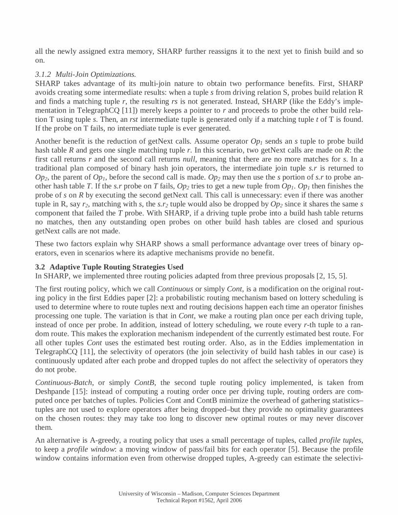
ties of operators even for routes that it never executes. This information is then used to provide strong guarantees on the optimality of routes that A-greedy selects [5]. However, A-greedy has a higher state update overhead then Cont or ContB and that is why it collects information just after every profile tuple, instead of after every tuple. A-greedy, developed for data stream scenarios where data and system char-acteristics are expected to change very quickly, computes a new routing order after every profile tuple. Since SHARP is processing local relations instead of data streams, and to lower the overhead of comput-ing routes and to produce the first routing order faster, our implementation of A-greedy, called Profile, uses the first n out of every p tuples as profile tuples. Thus, Profile, the third tuple routing policy imple-mented in SHARP, computes a new routing order after every n+K*p tuples, with K≥0, and uses that routing order for the next p driving tuples. Table 1 summarizes the routing policies implemented.

3.3 Late Binding Decisions In this Section we describe a series of late binding decisions–decisions made at run-time after some tu-ples are observed–that change the structure of the query plan executed by SHARP.

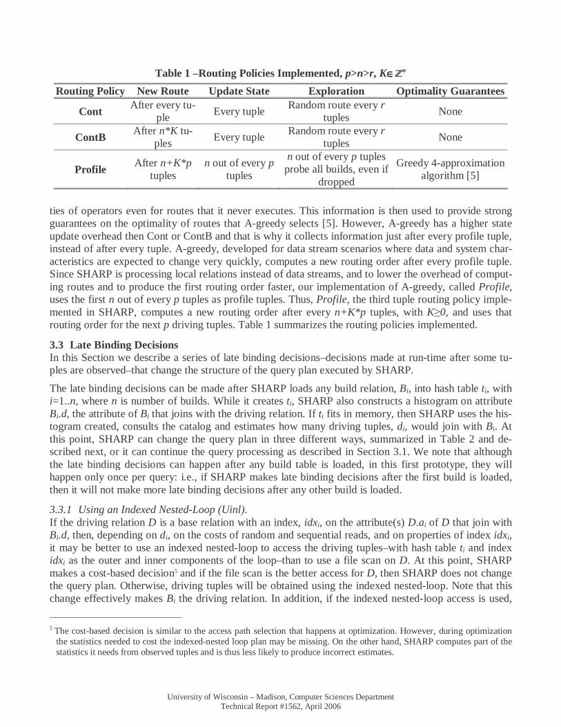
The late binding decisions can be made after SHARP loads any build relation, Bi, into hash table ti, with i=1..n, where n is number of builds. While it creates ti, SHARP also constructs a histogram on attribute Bi.d, the attribute of Bi that joins with the driving relation. If ti fits in memory, then SHARP uses the his-togram created, consults the catalog and estimates how many driving tuples, di, would join with Bi. At this point, SHARP can change the query plan in three different ways, summarized in Table 2 and de-scribed next, or it can continue the query processing as described in Section 3.1. We note that although the late binding decisions can happen after any build table is loaded, in this first prototype, they will happen only once per query: i.e., if SHARP makes late binding decisions after the first build is loaded, then it will not make more late binding decisions after any other build is loaded.

3.3.1 Using an Indexed Nested-Loop (Uinl). If the driving relation D is a base relation with an index, idxi, on the attribute(s) D.ai of D that join with Bi.d, then, depending on di, on the costs of random and sequential reads, and on properties of index idxi, it may be better to use an indexed nested-loop to access the driving tuples–with hash table ti and index idxi as the outer and inner components of the loop–than to use a file scan on D. At this point, SHARP makes a cost-based decision5 and if the file scan is the better access for D, then SHARP does not change the query plan. Otherwise, driving tuples will be obtained using the indexed nested-loop. Note that this change effectively makes Bi the driving relation. In addition, if the indexed nested-loop access is used,

5 The cost-based decision is similar to the access path selection that happens at optimization. However, during optimization

the statistics needed to cost the indexed-nested loop plan may be missing. On the other hand, SHARP computes part of the statistics it needs from observed tuples and is thus less likely to produce incorrect estimates.

Table 1 –Routing Policies Implemented, p>n>r, K∈∈∈∈

Routing Policy New Route Update State Exploration Optimality Guarantees

Cont After every tu-

ple Every tuple

Random route every r tuples

None

ContB After n*K tu-

ples Every tuple

Random route every r tuples

None

Profile After n+K*p

tuples n out of every p

tuples

n out of every p tuples probe all builds, even if

dropped

Greedy 4-approximation algorithm [5]


then the late binding decision “Using INL and Bloom-Filters”, below, is considered before any other build relation is processed.

3.3.2 Using INL and Bloom-Filters (Uibf). Given di and the average size of a driving tuple, SHARP computes the total expected size of those di tu-ples, Ti. If Ti is less than the budget given to any build hash table, then SHARP reads all the di driving tuples into memory before proceeding to read other builds. For each driving tuple it loads into memory, SHARP reads attribute aj that joins with build relation Bj and updates the a bloom filter bfj, for j=1..n, j≠i. Each bloom filter, bfj, is a bitmap of length k [9]. When driving tuples are read, attribute aj is hashed to a value between 0 and k-1, and the corresponding bit in bfj is set. Later, when the other build relations are read, for each tuple, SHARP hashes its join attribute, Bj.d, with the hash function used for bfj. If the bit corresponding to that value in bfj is 0, then the tuple is dropped, otherwise the tuple is processed nor-mally.

3.3.3 Using Driving Relation Pre-Filtering and Bloom Filters (Ufbf). As described in Section 3.4, SHARP’s second-stage processing requires a second pass on portions of the driving relation if any build relation requires a second pass. As such, filtering the build relations with bloom-filters may improve performance significantly because it could save both the builds and the driv-ing relations from spilling to disk. Thus, even if SHARP decides not to use an indexed nested-loop to retrieve the driving tuples, it will still check, after building any ti, if the Ti (the size of all tuples of D es-timated to match ti) fits the budget given to build hash tables. If it does, then, as in the case Uibf above, SHARP reads driving tuples into memory ahead of time. Each driving tuple read probes ti and if it finds no match, it is dropped. Otherwise, it is kept in an in-memory buffer and it is used to update bloom-filters on the other build relations. Then, build relations are loaded into memory while being filtered by the bloom-filters. Finally, driving tuples are read from the in-memory buffer, and used to probe the builds.

3.4 Second-Stage Processing Even after redistributing memory across joins (Section 3.1) and filtering tables using the late binding decisions (Section 3.3) it is still possible that one or more relations do not fit in memory. Those portions will have to be temporarily written to disk and processed at a later stage, typically referred to as second-stage. This Section describes SHARP’s second-stage processing algorithms.

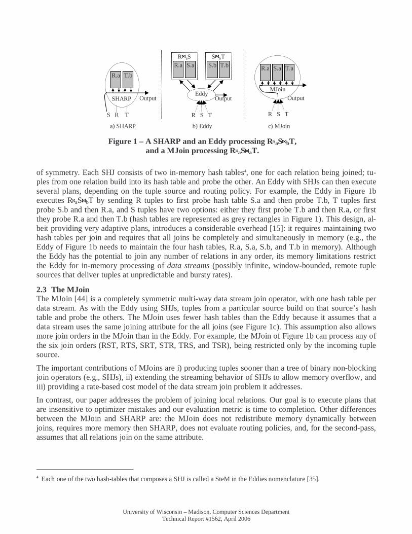
3.4.1 Split Tables into Partitions and Portions. When SHARP reads build relation Bi, it creates an in-memory hash table ti with p partitions. If there is no more memory space for Bi tuples, one in-memory partition of ti is selected, its current records are moved to a temporary file on disk, the partition is marked as frozen, and SHARP continues loading re-cords from Bi. Future records that hash to frozen partitions are held in very small memory buffers and flushed to disk when the buffers fill up. Then, for each ti, the partitions are assigned to sets of consecu-tive partitions called portions, such that the size of each portion does not exceed available memory. Figure 3a shows the state of a SHARP after it has completed the build stage. In the example, build hash

Table 2 – Summary of Late Binding Decisions

Decision Type of D Read D Access D Buffer D? Uinl Base After Bn Index No (stream) Uibf Base After Bi Index Yes Ufbf Base, intermediate After Bi Unchanged Yes


table t1 has four portions. Portion 0 is in memory, and the remaining three portions contain the frozen partitions.

After the builds are partitioned, SHARP reads the driving table and partitions it along all n join attributes with the build relations. This multi-dimensional split of D is shown in Figure 3b for the case of two build relations. Note that the split of D is done in terms of portions of the ti, instead of partitions of ti.

To split D, incoming driving tuples are routed to some ti for probing (according to SHARP’s routing policy as described in Section 3.2). When SHARP probes ti with driving tuple dt, using join attribute dt.ai, it gets one of three results: “match”, “fail”, or ti(dt.ai), the number of the in-disk partition of ti that dt.ai hashes to. We note that a “match” also includes the set of pointers to the dt matching tuples in ti and implicitly implies that portion ti(dt.ai) is in memory (i.e., ti(dt.ai)=0).

If any ti probe returns “fail”, tuple dt is dropped; otherwise the tuple is routed to another hash table. If dt is not dropped, there are three cases to consider, corresponding to the dotted, white, and gray portions of D in Figure 3b:

• If all ti probes return “match” (dt belongs to the dotted portion of D), then the resulting one or more join tuples are output by SHARP and not written for second-stage processing.

• If all ti(dt.ai)>0 (dt belongs to a white portion of D), then it is not known if tuple dt joins or not with any of the builds. Tuple dt is then written to a temporary file for second-stage processing.

• If at least one, but not all tables, ti returned “match” (ti(dt.ai)=0) then driving tuples dt belongs to a grey portion of D. In this situation, dt tuples can be processed in two ways: Save Intermediate Tuples (SIT) or Save Driving Tuples (SDT). In option SIT, SHARP writes to temporary files the intermedi-ate join between dt and its matching tuples (from the hash tables that returned “match”). In option SDT SHARP writes just dt to temporarily files and discards any matching tuples, which are then ob-tained again during the second-stage processing of dt.

When option SIT is used some D portions (marked gray in Figure 3b) will contain wider, intermediate join tuples, but the probing work will not be lost. When option SDT is used, all D portions contain just driving tuples, but the probing work will be lost and will have to be repeated later by reloading portions of build tables from disk. Depending on the relative sizes of driving tuples and their matching records, and on the selectivity of the joins, either option can be better. Furthermore, the choice between SIT and SDT made for driving tuples for which ti(dt.ai)=0 can be different of the choices between SIT and SDT for tuples for which tj(dt.aj)=0, j≠i. For example, in Figure 3b, choice SIT can be used for D portions marked 4, 6 and 8, and option SDT can be used for D portions 11 and 20. To simplify the second-stage algorithm, the prototype implementation of SHARP always uses option SDT.

Memory

Disk

t1 t2

Figure 3 – Second stage processing

a) End of build stage

t2

t1

D b) Multi-dimensional

split of D

0

1

2

0

1

2

3

1

2,10,... 3,…

4

5,… 7,…

6 8

13 15 17 9 11

18 22 24 26 20

Portions

Partitions …


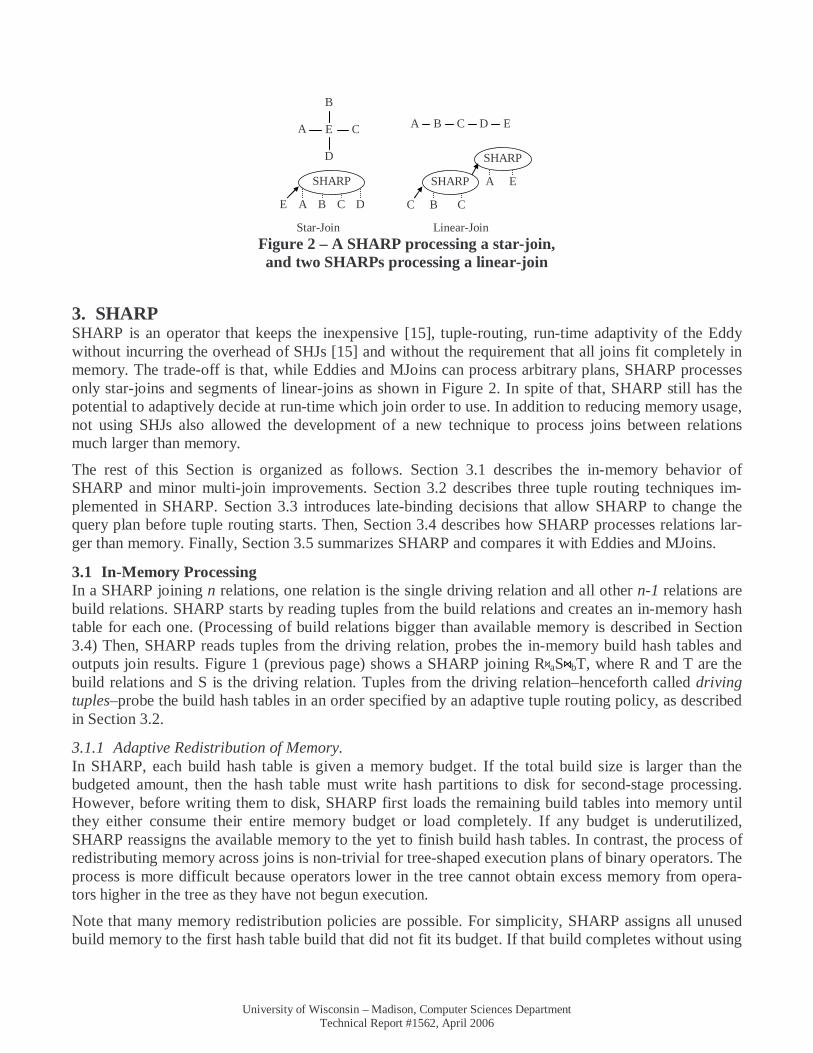
Figure 5 – Right-Deep Tree of DHJs D B1

DHJ B2

DHJ B3

DHJ

3.4.2 Second-stage Joins. After the multi-dimensional split of D is complete, SHARP begins the second-stage of the join. First SHARP orders the build hash tables based on the ascending number of portions and, if there is a tie, based on their descending total size. This order is represented by O(i), such that O(i) represents the i-th build hash table in the order. In the example of Figure 3, O(1)=t2 and O(2)=t1 because t2 has just three por-tions while t1 has four portions. Assume also that |O(i)| represents the number of portions in hash table O(i) and that O(i).load(k) loads portion k, with k<|O(i)| of hash table O(i) into memory, deleting from memory the current in-memory portion of O(i) and that function Dportion(i1, i2, …, in) returns the portion of D that corresponds to the i1-th portion of O(1), to the i2-th portion of O(2), …, and to the in-th portion of O(n). In the example of Figure 3, Dportion(1,2) corresponds to the portion of D marked with a circle.

Then, as shown in the pseudo-code of Figure 4, SHARP executes a series of loops, loading portions of O(1) to O(n) into memory, getting tuples from the corresponding D portion, probing the in-memory por-tions of O(1) to O(n) and outputting matches. This algorithm loads the on-disk portions of D one time and loads the in-disk portions of O(i) a number of times equal to ∏j=1..i-1|O(j)|. The numbers in Figure 3b rep-resent the order in which portions of the example of Figure 3a are loaded.

for (i1=0; i1<|O(1)|, O(1).load(i1); i1++) for (i2=0; i2<|O(2)|, O(2).load(i2); i2++) … for (in=0; in<|O(n)|, O(n).load(in); in++) for all tuples dt in Dportion(i1, i2, …, in) dt probes in-memory portions of O(i), …, O(n); output matches between dt and O(i), …, O(n); end for; end for; … end for; end for;

Figure 4 – Second-stage Pseudo Code

In contrast, a right deep tree of binary dynamic hash joins, reads each input relation just once, but may have to save to and read from disk (during the second-stage processing) the intermediate results multiple times. For example, if no Bi, i=1,2,3 fits completely in memory, the execution plan corresponding to the right-deep tree of Figure 5 will need to do a second-pass for each of the joins, saving to and reading from disk part of the intermediate results corresponding to D B1, D B1 B2, and D B1 B2 B3. To mini-mize the size of those intermediate results, an accurate optimizer estimates the join selectivities between D and Bi, and other things being equal, sets D’s join order to be from the most to the least selective Bi. However, join selectivities are hard to estimate correctly and an optimizer may choose an incorrect join order which negatively affects performance.


On the other hand, the performance of SHARP depends very little on the join order defined by the opti-mizer. If the builds fit in memory, the join order is determined by an adaptive tuple routing policy at run-time. If the builds do not fit in memory, the cost of SHARP’s second-stage depends mainly on the order O(i), but this order is determined only after all build tuples are observed; no estimates are needed. However, the performance of SHARP’s second-stage suffers from the “curse of dimensionality”: if sev-eral build relations are much larger than memory, then the repeated readings of the inner most build, O(n), (which is read ∏i=1..n-1|O(i)| times) may dominate the total cost of the join. In the Experimental Evaluation Section we explore how the available memory affects the performance of SHARP. It is also shown that even with an amount of available memory equal to just 10% the size of the largest build ta-ble, SHARP’s second-stage can still outperform other methods.

3.5 Summary of SHARP SHARP does not use symmetry plans (like the MJoin) nor symmetric operators (like the Eddy).and in-stead of allowing all relations to be used as builds or probes, the optimizer chooses one single driving relation. Since only build relations have hash tables, this design reduces the memory footprint of a SHARP to essentially half of what an Eddy and its SHJs would consume. The routing policy is then re-sponsible for determining the order with which driving tuples probe the build sources.

By having a single driving relation, routing policies in SHARP have fewer routes to choose from than in Eddies (because routing decisions affect only tuples coming from driving relations). However, because SHARP is a pull-based operator–in charge of obtaining new tuples from its sources–we were able to de-sign a series of late binding decisions that, in some cases, are able to promote any of the builds to be the driving relation before the tuple routing stage starts.

In short, an Eddy is able to change execution from any route to any other route at any stage of execution, while a SHARP first determines which source is the driving relation and then continuously adapts the sequence in which the driving tuples probe the build sources. With this two-step adaptive process, SHARP still has the potential to adaptively decide at run-time which one of all6 possible join orders to use but with a much smaller memory footprint.

4. EXPERIMENTAL EVALUATION We now describe an experimental evaluation of the query processing techniques described for SHARP using a prototype implementation in Predator [38]. All results were obtained using a dedicated machine with 512 MB of main memory and a buffer pool of 2000 16-Kbyte pages (hash table builds are kept out-side the buffer pool). Results are averages of three to five cold runs.

We note that the first experimental results (Section 4.2) do not evaluate any adaptivity feature of SHARP and exhibit only marginal improvements of a SHARP over competing plans. The purpose of that Section, though, is twofold. First, we want to show that, not only is the adaptivity overhead of SHARP very low, but also, even in scenarios where the adaptivity yields no benefit, SHARP still pro-vides a marginal performance advantage due to its multi-join nature. Second, the adaptivity benefits of SHARP compound these initial multi-join improvements.

4.1 Datasets The SHARP prototype was evaluated using two datasets, Star and TPCH, described below. Star, a syn-thetic dataset we created, allowed us to more easily explore different selectivities, join selectivities and

6 Ignoring join orders using Cartesian products.


table sizes. TPCH is used to evaluate SHARP’s adaptivity and robustness in a widely known bench-mark:

• Star: We created a synthetic benchmark, Star, based on a star schema, with a central fact table F, and four dimension tables, A, B, C, and D. F has 1,000,000 152-byte records and A, B, C, and D have 100,000 40-byte records. Our experiments use 2-way, 3-way, and 4-way join queries of the following form:

SELECT * FROM F, A, B, …, D WHERE F.fkdA = A.pk AND F.fkdB = B.pk … AND F.fkdD = D.pk AND σ1(A) AND σ2(B) … AND σ4(C); Where σi, i=1,..,4 represent selection predicates with selectivities between 0% and 100%.

• TPC-H: TPC-H is the decision support benchmark from the Transaction Processing Performance Council [40]. We used tables lineitem (L), orders (O), part (P), customer (C), and supplier (S), with scale size 1. We included an extra column in L (a foreign-key to C) to allow star-schema queries using one central fact table (L) and up to four dimension tables (O, P, C, and S). Our queries join either all tables, or all except O (the largest dimension), or all except S (the smallest dimension), and we use varying selection predicates on the dimension tables.

4.2 Evaluating Multi-Join Improvements As described in Section 3.1, SHARP has two benefits over plans composed of a tree of binary operators: it can avoid unnecessary intermediate tuple generation and unnecessary getNext calls. We note that these benefits are not due to any adaptive feature of SHARP. Instead, they are a positive side effect of the multi-join nature of SHARP.

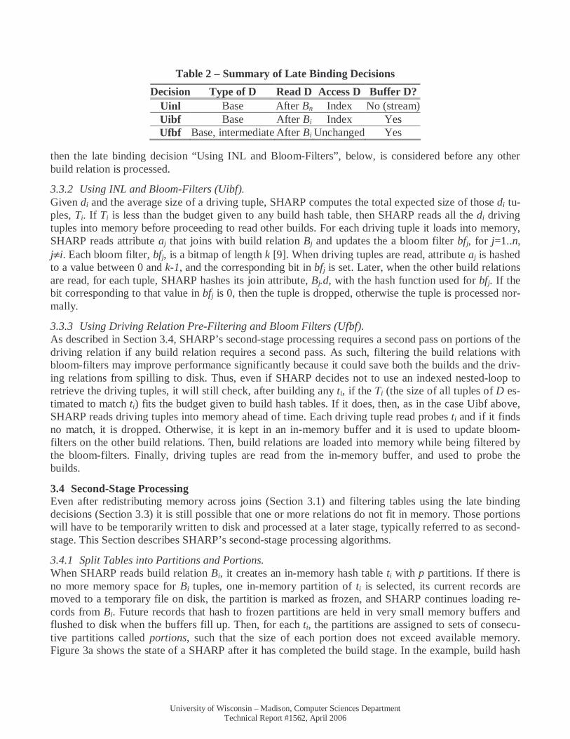
In the results shown in Figure 6, table F from schema Star, was joined with two, three, and four dimen-sion tables. All the dimension tables fit in memory, and all join selectivities7 are 100%. We compare three execution plans: SHARP, SHARP-IR, and RDH. SHARP-IR is a variation of SHARP that gener-ates intermediate join tuples after each successful probe. RDH is a plan composed of a right-deep tree of dynamic hash joins [33], with F as the rightmost table8 as shown in Figure 11. Both SHARP and SHARP-IR have their run-time statistics collection and adaptive routing policies turned off to ensure that the probing sequence is the same in all plans, and to ensure that we are measuring just the multi-join benefits. (The performance of routing policies in measured in Section 4.4.) All three plans use the same hash table implementation code. The benefit of avoiding intermediate results varies between 5% and 15%.

7 We use the term join selectivity of a build table as the average number of returned records per probing record. 8 The right-deep tree plan creates hash tables on the same relations and executes the same number of build and probe opera-

tions as SHARP.


In a second experiment, we set the selectivity of the last join to 0% (e.g., for the case of three joins, 100% of F tuples join with the first and second dimension, and 0% join with the third dimension). These contrived plans maximize the number of spurious getNext calls made by the RDH plan and give an up-per bound on the benefit obtained by avoiding those calls. Figure 8 shows the results for SHARP, SHARP-IR and RDH: SHARP is between 10% and 23% faster than RDH and SHARP-IR is around 5% faster than RDH.

The results show that, even without taking advantage of adaptivity, a tuple routing operator can slightly outperform plans composed of a tree of binary operators.

4.3 Redistributing Memory Between Joins For each query, our system gives a pre-specified memory budget for each hash table used to implement hash joins. Traditionally, if building the hash table requires more memory space than the memory budget, some partitions would have to be written to disk and a second-pass on those partitions would be required. In addition, if the hash table requires less memory than the allocated budget, then the unused memory–save some exceptions [14]–is not given to other operators. On the other hand, as described in Section 3.1, SHARP loads all its builds into memory before reading the driving relation and is therefore able to redistribute memory between different hash tables.

To evaluate the impact of memory redistribution, table F was joined with selections σ1 and σ2 on tables A and B. The selections are such that the size of σ2(B), |σ2(B)|, is four times the size of σ1(A), |σ1(A)|, and (|σ1(A)|+|σ2(B)|)/2 is equal to the memory budget for hash tables. Thus, σ1(A) underutilizes its budget while σ2(B) overutilizes it, but on average both fit in memory.

Four different plans were tested, for the four combinations of using SHARP and a RDH and of using two join orders, joining F with A first and then with B, or joining F with B first and then with A. Then, as shown in Figure 7, the size of the combined memory budget was varied from |σ1(A)|+|σ2(B)| (corre-sponds to 100%) to 2*|σ2(B)| (160%).

SHARP is able to take advantage of memory redistribution and avoid a second-stage for all amounts of memory tested. On the other hand, because the RDH executes a tree of independent operators, it does not redistribute memory amongst the operators. Thus, the RDH plan only avoids a second-pass in both operators when the budget per hash table is at least as large as the largest hash table. This happens only for a combined memory budget of 2*|σ2(B)|, or 160% the size of the |σ1(A)|+|σ2(B)|. If more than 2*|σ2(B)| of memory is available, the performance of all four plans remains unaffected. If less than

Figure 8 – Avoiding getNext Calls

Figure 6 – Avoiding Intermediate Results

Figure 7 – Redistributing Memory

0

10

20

30

3 4 5Number of tables joined

RDHSHARP-IRSHARP

Secs.

0

10

20

30

3 4 5Number of tables joined

RDHSHARP-IRSHARP

Secs.

0

10

20

30

40

100% 120% 140% 160%% of builds that fit in memory

RDH-BARDH-ABSHARP-BASHARP-AB

Secs.


Figure 10 – Low Profiling Overhead, High Probing Cost

|σ1(A)|+|σ2(B)| of memory is available, SHARP also needs a second-stage. Experiments showing the performance of the SHARP second-stage appear in Section 4.5.

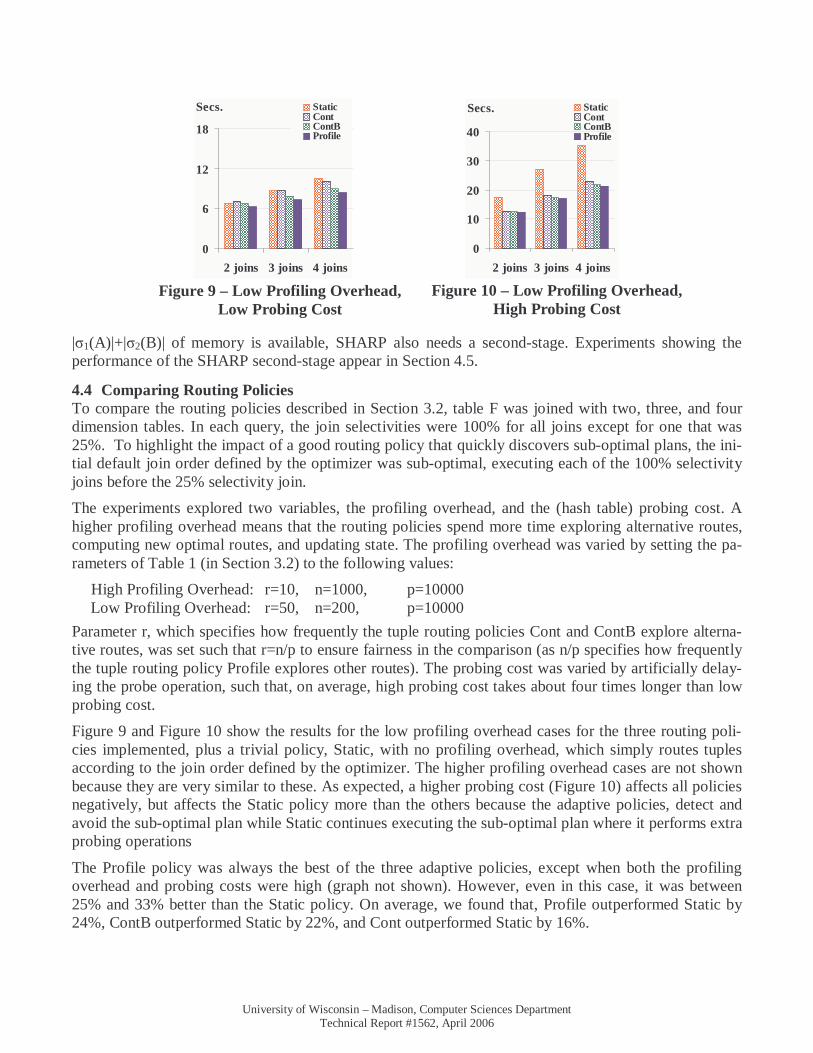
4.4 Comparing Routing Policies To compare the routing policies described in Section 3.2, table F was joined with two, three, and four dimension tables. In each query, the join selectivities were 100% for all joins except for one that was 25%. To highlight the impact of a good routing policy that quickly discovers sub-optimal plans, the ini-tial default join order defined by the optimizer was sub-optimal, executing each of the 100% selectivity joins before the 25% selectivity join.

The experiments explored two variables, the profiling overhead, and the (hash table) probing cost. A higher profiling overhead means that the routing policies spend more time exploring alternative routes, computing new optimal routes, and updating state. The profiling overhead was varied by setting the pa-rameters of Table 1 (in Section 3.2) to the following values:

High Profiling Overhead: r=10, n=1000, p=10000 Low Profiling Overhead: r=50, n=200, p=10000

Parameter r, which specifies how frequently the tuple routing policies Cont and ContB explore alterna-tive routes, was set such that r=n/p to ensure fairness in the comparison (as n/p specifies how frequently the tuple routing policy Profile explores other routes). The probing cost was varied by artificially delay-ing the probe operation, such that, on average, high probing cost takes about four times longer than low probing cost.

Figure 9 and Figure 10 show the results for the low profiling overhead cases for the three routing poli-cies implemented, plus a trivial policy, Static, with no profiling overhead, which simply routes tuples according to the join order defined by the optimizer. The higher profiling overhead cases are not shown because they are very similar to these. As expected, a higher probing cost (Figure 10) affects all policies negatively, but affects the Static policy more than the others because the adaptive policies, detect and avoid the sub-optimal plan while Static continues executing the sub-optimal plan where it performs extra probing operations

The Profile policy was always the best of the three adaptive policies, except when both the profiling overhead and probing costs were high (graph not shown). However, even in this case, it was between 25% and 33% better than the Static policy. On average, we found that, Profile outperformed Static by 24%, ContB outperformed Static by 22%, and Cont outperformed Static by 16%.

Figure 9 – Low Profiling Overhead, Low Probing Cost

0

6

12

18

2 joins 3 joins 4 joins

StaticContContBProfile

Secs.

0

10

20

30

40

2 joins 3 joins 4 joins

StaticContContBProfile

Secs.


4.5 Evaluating the Second-Stage To evaluate the performance of the second-stage processing of SHARP, we joined tables F, A, and B in one query and tables F, A, B, C, and D in another query. (Further experiments in the next two Sections also evaluate the second-stage.) The amount of memory was varied such that between 10% and 100% of tables A and B in the first query, and A, B, C, and D in the second would fit in memory. SHARP was compared with plans RDH and LDH. We note that both SHARP and the RDH plan are non-blocking plans, and therefore, their execution pipeline uses the in-memory parts of all the build hash tables simul-taneously (see Figure 11b showing RDH’s execution pipeline in gray). In contrast, the execution pipe-line of LDH plan, at any moment only manipulates two hash tables (see Figure 11c). Thus, to ensure the amount of total memory per plan was the same, hash tables in the LDH plan were allowed twice the memory of hash tables in SHARP and the RDH plans. The results are shown in Figure 12 and Figure 13.

Except when the amount of memory is very limited, SHARP outperforms the other two plans. If several build relations are much larger than memory, then the innermost build will be read many times and the performance of SHARP degrades quickly. On the other hand, as shown in Section 4.7, if just one or two builds are much larger than memory, and the remaining builds either fit in memory or are not much lar-ger than memory, then the performance of SHARP degrades much more slowly.

To address the exponential degradation problem, the SHARP could convert itself to a RDH plan: after all the builds are read and partitioned, SHARP can easily determine if its performance will degrade quickly or not. At this point, the conversion to a RDH plan is essentially free; all dimension tables are already partitioned with the right hash functions, and no work is lost. We leave this late binding decision that as future work.

0

50

100

150

0% 20% 40% 60% 80% 100%Percentage of builds that fit in memory

LDHRDHSHARP

Secs.

Figure 12 – Evaluating Second-Stage, 2 joins

Figure 11 – a) SHARP; b) right-deep tree of DHJs; c) left-deep tree of DHJs

c) LDH Plan F A

DHJ

a) SHARP Plan

D C B A F

SHARP

B

DHJ C

DHJ D

DHJ

b) RDH Plan F A

DHJ B

DHJ C

DHJ D

DHJ


0

250

500

0% 20% 40% 60% 80% 100%Percentage of builds that fit in memory

LDHRDHSHARP

Secs.

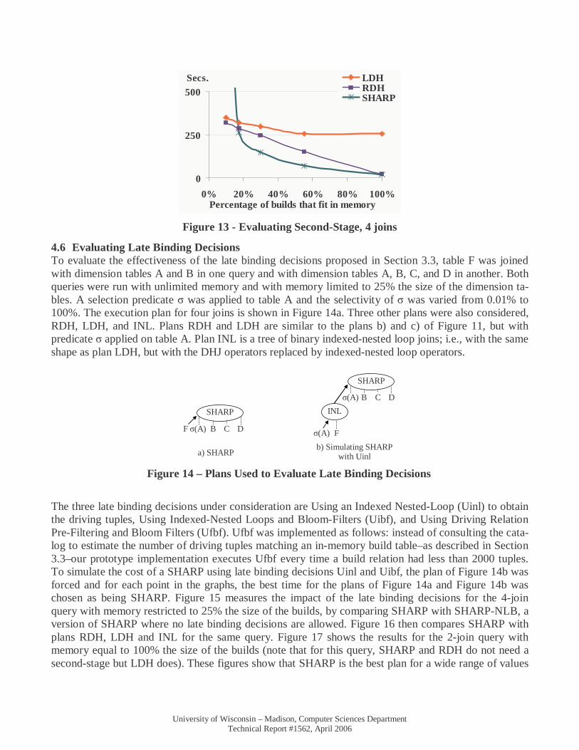
Figure 13 - Evaluating Second-Stage, 4 joins

4.6 Evaluating Late Binding Decisions To evaluate the effectiveness of the late binding decisions proposed in Section 3.3, table F was joined with dimension tables A and B in one query and with dimension tables A, B, C, and D in another. Both queries were run with unlimited memory and with memory limited to 25% the size of the dimension ta-bles. A selection predicate σ was applied to table A and the selectivity of σ was varied from 0.01% to 100%. The execution plan for four joins is shown in Figure 14a. Three other plans were also considered, RDH, LDH, and INL. Plans RDH and LDH are similar to the plans b) and c) of Figure 11, but with predicate σ applied on table A. Plan INL is a tree of binary indexed-nested loop joins; i.e., with the same shape as plan LDH, but with the DHJ operators replaced by indexed-nested loop operators.

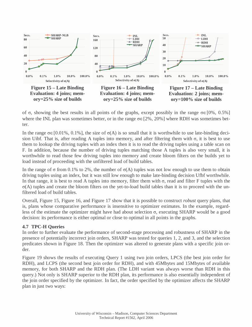
The three late binding decisions under consideration are Using an Indexed Nested-Loop (Uinl) to obtain the driving tuples, Using Indexed-Nested Loops and Bloom-Filters (Uibf), and Using Driving Relation Pre-Filtering and Bloom Filters (Ufbf). Ufbf was implemented as follows: instead of consulting the cata-log to estimate the number of driving tuples matching an in-memory build table–as described in Section 3.3–our prototype implementation executes Ufbf every time a build relation had less than 2000 tuples. To simulate the cost of a SHARP using late binding decisions Uinl and Uibf, the plan of Figure 14b was forced and for each point in the graphs, the best time for the plans of Figure 14a and Figure 14b was chosen as being SHARP. Figure 15 measures the impact of the late binding decisions for the 4-join query with memory restricted to 25% the size of the builds, by comparing SHARP with SHARP-NLB, a version of SHARP where no late binding decisions are allowed. Figure 16 then compares SHARP with plans RDH, LDH and INL for the same query. Figure 17 shows the results for the 2-join query with memory equal to 100% the size of the builds (note that for this query, SHARP and RDH do not need a second-stage but LDH does). These figures show that SHARP is the best plan for a wide range of values

Figure 14 – Plans Used to Evaluate Late Binding Decisions

a) SHARP

D C B σ(A) F

SHARP

b) Simulating SHARP with Uinl

F

INL

D C B

SHARP

σ(A)

σ(A)


of σ, showing the best results in all points of the graphs, except possibly in the range σ∈[0%, 0.5%] where the INL plan was sometimes better, or in the range σ∈[2%, 20%] where RDH was sometimes bet-ter.

In the range σ∈[0.01%, 0.1%], the size of σ(A) is so small that it is worthwhile to use late-binding deci-sion Uibf. That is, after reading A tuples into memory, and after filtering them with σ, it is best to use them to lookup the driving tuples with an index then it is to read the driving tuples using a table scan on F. In addition, because the number of driving tuples matching those A tuples is also very small, it is worthwhile to read those few driving tuples into memory and create bloom filters on the builds yet to load instead of proceeding with the unfiltered load of build tables.

In the range of σ from 0.1% to 2%, the number of σ(A) tuples was not low enough to use them to obtain driving tuples using an index, but it was still low enough to make late-binding decision Ufbf worthwhile. In that range, it is best to read A tuples into memory, filter them with σ, read and filter F tuples with the σ(A) tuples and create the bloom filters on the yet-to-load build tables than it is to proceed with the un-filtered load of build tables.

Overall, Figure 15, Figure 16, and Figure 17 show that it is possible to construct robust query plans, that is, plans whose comparative performance is insensitive to optimizer estimates. In the example, regard-less of the estimate the optimizer might have had about selection σ, executing SHARP would be a good decision: its performance is either optimal or close to optimal in all points in the graphs.

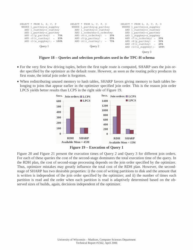
4.7 TPC-H Queries In order to further evaluate the performance of second-stage processing and robustness of SHARP in the presence of potentially incorrect join orders, SHARP was tested for queries 1, 2, and 3, and the selection predicates shown in Figure 18. Then the optimizer was altered to generate plans with a specific join or-der.

Figure 19 shows the results of executing Query 1 using two join orders, LPCS (the best join order for RDH), and LCPS (the second best join order for RDH), and with 45Mbytes and 15Mbytes of available memory, for both SHARP and the RDH plan. (The LDH variant was always worse than RDH in this query.) Not only is SHARP superior to the RDH plan, its performance is also essentially independent of the join order specified by the optimizer. In fact, the order specified by the optimizer affects the SHARP plan in just two ways:

0

20

40

60

80

0.0% 0.1% 1.0% 10.0% 100.0%

Selectivity of σ(A)

SHARP-NLBSHARP

Secs.

0

40

80

120

160

0.0% 0.1% 1.0% 10.0% 100.0%Selectivity of σ(A)

INLLDHRDHSHARP

Secs.

0

10

20

30

40

50

0.0% 0.1% 1.0% 10.0% 100.0%

Selectivity of σ(A)

INLLDHRDHSHARP

Secs.

Figure 15 – Late Binding Evaluation: 4 joins; mem-

ory=25% size of builds

Figure 16 – Late Binding Evaluation: 4 joins; mem-

ory=25% size of builds

Figure 17 – Late Binding Evaluation: 2 joins; mem-ory=100% size of builds


• For the very first few driving tuples, before the first tuple route is computed, SHARP uses the join or-der specified by the optimizer as the default route. However, as soon as the routing policy produces its first route, the initial join order is forgotten.

• When redistributing unused memory to hash tables, SHARP favors giving memory to hash tables be-longing to joins that appear earlier in the optimizer specified join order. This is the reason join order LPCS yields better results than LCPS in the right side of Figure 19.

Join orders:

0

100

200

300

400

500

600

RDH SHARPAvailable Mem = 45M

LCPSLPCS

Secs.

Join orders:

0

200

400

600

800

1000

1200

1400


LCPSLPCS

Secs.

Figure 19 – Execution of Query 1

Figure 20 and Figure 21 present the execution times of Query 2 and Query 3 for different join orders. For each of these queries the cost of the second-stage dominates the total execution time of the query. In the RDH plan, the cost of second-stage processing depends on the join order specified by the optimizer. Thus, optimizer mistakes may greatly influence the total cost of the RDH plan. However, the second-stage of SHARP has two desirable properties: i) the cost of writing partitions to disk and the amount that is written is independent of the join order specified by the optimizer; and ii) the number of times each partition is read and the order when each partition is read is adaptively determined based on the ob-served sizes of builds, again, decisions independent of the optimizer.

SELECT * FROM L, S, C, P WHERE l_partkey=s_suppkey AND l_custkey=c_custkey AND l_partkey=o_partkey AND σ1(p_partkey) ← 75% AND σ2(c_custkey) ← 25% AND σ3(s_suppkey); ← 100%

Query 1

SELECT * FROM L, C, P, O WHERE l_partkey=p_partkey AND l_custkey=c_custkey AND l_orderkey=o_orderkey AND σ4(o_orderkey) ← 25% AND σ5(p_partkey) ← 25% AND σ6(c_custkey); ← 75%

Query 2

SELECT * FROM L, S, C, P, O WHERE l_partkey=s_suppkey AND l_custkey=c_custkey AND l_partkey=o_partkey AND l_suppkey=s_suppkey AND σ7(o_orderkey) ← 25% AND σ8(p_partkey) ← 50% AND σ9(c_custkey) ← 25% AND σ10(s_suppkey);← 100%

Query 3

Figure 18 – Queries and selection predicates used in the TPC-H schema


Join orders:

0

400

800

1200


CPOPCOPOC

Secs.

Join orders:

0

250

500

750

RDH SHARP

Available Mem = 10M

COPSCPOSOCPSSCOP

Secs.

For the queries we run, RDH can take twice as long in a join order for a query then in another join order for the same query. In addition, across all experiments (some experiments not shown), RDH took on av-erage twice as long as SHARP to complete execution.

Finally, we created a variation of the TPC-H schema, which we call TPC-H-Thin, to explore how the width of the tuples affects SHARP’s relative performance. Each table in TPC-H-Thin is a projection of the corresponding table in TPC-H: table L contains only five integer columns, and tables O, P, C, and S contain only two integer columns. We run queries 1, 2, and 3 again, but this time with much less avail-able memory, such that not all build tables fit in memory. The results are similar to the ones shown in Figure 19, Figure 20, and Figure 21; SHARP is essentially insensitive to the join order specified by the optimizer while the RDH may time up to 3 times longer in one join order than in another join order for the same query. Furthermore, for the queries we run in TPC-H-Thin, RDH took on average 2.2 times longer than SHARP to complete execution.

5. RELATED WORK In addition to the Eddies, MJoin and SHJ operators described in Section 2, the work related to SHARP can be grouped in five broad categories: adaptive operators, tuple routing strategies, techniques for proc-essing joins larger than memory, techniques to change the query plan at run-time, and techniques that reduce the need for corrective behavior.

Other adaptive operators: The XJoin [42] is a binary adaptive operator that takes advantage of the non-blocking behavior of SHJ to process push-based remote relations. Although it can process relations bigger than memory, the XJoin schedules the join between out-of-memory relations to mask delays and bursty transfer rates of those sources. In contrast, SHARP uses adaptivity to execute robust plans over pull-based local relations. The operators most related to SHARP’s late-binding decisions are the choose-plan operator [13, 18] and the switchable plan operator [7], but neither provides the continuous fine-grained adaptivity of SHARP.

Tuple routing strategies: In SHARP, we implemented three routing policies adapted from three pro-posals by Avnur [2], Babu [5], and Deshpande [15]. CBR is a tuple routing policy that takes advantage of correlation and skew to make better routing decisions [8]. The implementation of CBR in SHARP is left as future work.

Techniques for processing joins larger than memory: The Dynamic Hash Join (DHJ) [33] is the stan-dard blocking binary hash join algorithm that adaptively freezes partitions to disk as needed and that we

Figure 20 – Execution of Query 2 Figure 21 – Execution of Query 3


extended to join multiple relations simultaneously. The XJoin [42] and Ives [27] proposed techniques extending the SHJ to process relations bigger than memory. However, these techniques were designed for binary joins over remote sources while SHARP processes multiple joins over local relations.

Changing query plan at run-time: In addition to the late-binding operators discussed before, there are proposals that use query re-optimization to correct possible optimizer mistakes [7, 27, 28, 30, 32]. These strategies are orthogonal to SHARP, i.e., a SHARP can be used as an adaptive operator in plans gener-ated by those systems. Other proposals keep the same query plan, but reschedule operators to cope with unpredictable delivery rates from remote data sources [10, 27, 28, 41, 42, 44] or to improve estimates for online queries [19¸20, 29]. In contrast, SHARP reschedules operators to better distribute memory be-tween in-memory hash tables and possibly avoid a second pass. (A method to redistribute memory in traditional query plans is described in [14].) Finally, some data stream systems periodically determine and change to new query plans [5, 16], and these strategies can be incorporated in SHARP as routing policies (e.g., we implemented [5] in SHARP).

Techniques that reduce the need for run-time corrective adaptivity: Other approaches tackle the problem of insufficient information available to the optimizer by somehow modeling the uncertainty about estimates used at optimization [3, 7, 18, 24, 43]. Optimizers following this approach are more likely to choose robust plans and therefore less likely to need corrective adaptation at run-time. Due to the complexity of the search space, we believe that a combination of some of these techniques, together with adaptive operators like SHARP will prove to be the best approach.

More related work can be found in surveys and other publications with extended discussion of related work [4, 6, 21, 25, 27, 28, 32].

6. CONCLUSIONS The observation that tuple routing is not expensive, but symmetric hash joins are [15] led us to design SHARP, a multi-join tuple routing operator without symmetric hash joins (SHJs). To avoid SHJs, we explored a new trade-off: instead of executing arbitrarily query plans, and being able to change from any join order to any other join order at any point during execution, SHARP adopts a two-step adaptive ap-proach. First, SHARP determines which source is the driving relation using late-binding decisions, and second, it continuously potentially changes the probing sequence of the build sources using tuple rout-ing. This two-step adaptive process yields two benefits: it requires less memory than previous adaptive operators and simplifies the design of second-stage processing.

In addition, the performance of the second-stage processing strategy is largely unaffected by estimates made during optimization. The second-stage was shown to be more effective than both left-deep and right-deep trees for a variety of scenarios. Most of the benefit of the proposed second-stage comes from avoiding writing intermediate results multiple times to disk. However, this new second-stage processing technique suffers from the “curse of dimensionality”, and thus beyond certain parameters (very little memory, very large build tables, or a high number of joins), we expect its performance to degrade expo-nentially. Nevertheless, the problem is easily solved: after all build tables are read, if the sizes of mem-ory and tables are such that the SHARP’s (second-stage) performance is worse than a right-deep tree of hash joins, then the SHARP can simply execute the same plan a right-deep tree of hash joins would.

In addition, our initial results suggest that, unless the operator processing cost is very high, the A-Greedy [5] tuple routing policy is likely to be the best.


7. REFERENCES [1] R. Arpaci-Dusseau. Run-time adaptation in river. ACM Trans. on Computer Systems, 21(1):36–86,

2003.

[2] R. Avnur and J. M. Hellerstein. Eddies: Continuously Adaptive Query Processing. In Proc. of the 2000 ACM SIGMOD Intl. Conf. on Management of Data, May 2000.

[3] B. Babcock and S. Chaudhuri. Towards a Robust Query Optimizer: A Principled and Practical Approach. In Proc. of the 2005 ACM SIGMOD Intl. Conf. on Management of Data, Jun 2005.

[4] B. Babcock, S. Babu, M. Datar, R. Motwani, J. Widom. Models and Issues in Data Stream Systems. PODS 2002: 1-16.

[5] S. Babu, R. Motwani, K. Munagala, I. Nishizawa, and J. Widom. Adaptive ordering of pipelined stream filters. In Proc. of the 2004 ACM SIGMOD Intl. Conf. on Management of Data, Jun 2004.

[6] S. Babu and P. Bizarro. Adaptive Query Processing in the Looking Glass. In Proc. of Second Biennial Conf. on Innovative Data Systems Research (CIDR), Jan 2005.

[7] S. Babu, P. Bizarro, and D. DeWitt. Proactive Re-optimization. In Proc. of the 2005 ACM SIGMOD Intl. Conf. on Management of Data, Jun 2005.

[8] P. Bizarro, S. Babu, D. DeWitt, and J. Widom. Content-Based Routing: Different Plans for Different Data. In Proc. of the 2005 Intl. Conf. on Very Large Data Bases, Sep 2005.

[9] Burton H. Bloom. Space/Time Trade-offs in Hash Coding with Allowable Errors. Commun. ACM 13(7): 422-426 (1970).

[10] L. Bouganim, F. Fabret, C. Mohan, P. Valduriez. A Dynamic Query Processing Architecture for Data Integration Systems. IEEE Data Eng. Bull. 23(2): 42-48 (2000).

[11] S. Chandrasekaran, O. Cooper, A. Deshpande, M. J. Franklin, J. M. Hellerstein, W. Hong, S. Krishnamurthy, S. Madden, V. Raman, F. Reiss, and M. Shah. TelegraphCQ: Continuous dataflow processing for an uncertain world. In Proc. First Biennial Conf. on Innovative Data Systems Research (CIDR), Jan 2003.

[12] F. Chu, J. Halpern, and P. Seshadri. Least expected cost query optimization: An exercise in utility. In Proc. of the 1999 ACM Symp. on Principles of Database Systems, 1999.

[13] R. L. Cole and G. Graefe. Optimization of dynamic query evaluation plans. In Proc. of the 1994 ACM SIGMOD Intl. Conf. on Management of Data, Jun 1994.

[14] B. Dageville and M. Zait. SQL memory management in Oracle9i. In Proc. of the 2002 Intl. Conf. on Very Large Data Bases, Aug. 2002.

[15] A. Deshpande. An initial study of overheads of eddies. SIGMOD Record 33(1): 44-49 (2004)

[16] A. Deshpande and J. M. Hellerstein. Lifting the Burden of History from Adaptive Query Processing. In Proc. of the 2004 Intl. Conf. on Very Large Data Bases, Sep 2004.

[17] S. Ganguly. Design and analysis of parametric query optimization algorithms. In Proc. of the 1998 Intl. Conf. on Very Large Data Bases, Aug. 1998.

[18] G. Graefe and K. Ward. Dynamic Query Evaluation Plans. In Proc. of the 1989 ACM SIGMOD Intl. Conf. on Management of Data, Jun 1989.

[19] P. Haas and J. M. Hellerstein. Ripple Joins for Online Aggregation. In Proc. of the 1999 ACM SIGMOD Intl. Conf. on Management of Data, Jun 1999.


[20] J. M. Hellerstein, P. Haas and H. J. Wang. Online Aggregation. In Proc. of the 1997 ACM SIGMOD Intl. Conf. on Management of Data, Jun 1997.

[21] J. M. Hellerstein, M. J. Franklin, et al. Adaptive query processing: Technology in evolution. IEEE Data Engineering Bulletin, 23(2):7–18, June 2000.

[22] A. Hulgeri and S. Sudarshan. AniPQO: Almost nonintrusive parametric query optimization for nonlinear cost functions. In Proc. of the 2003 Intl. Conf. on Very Large Data Bases, Aug. 2003.

[23] Y. Ioannidis and S. Christodoulakis. On the Propagation of Errors in the Size of Join Results. In Proc. of the 1991 ACM SIGMOD Intl. Conf. on Management of Data, May 1991.

[24] Y. Ioannidis, R. Ng, K. Shim, and T. Sellis. Parametric Query Optimization. In Proc. of the 1992 Intl. Conf. on Very Large Data Bases, Aug. 1992.

[25] Z. Ives. Efficient Query Processing for Data Integration. PhD thesis, University of Washington, Seattle, WA, USA, Aug. 2002.

[26] Z. Ives, D. Florescu, M. Friedman, A. Levy, D. Weld. An Adaptive Query Execution System for Data Integration. In Proc. of the 1999 ACM SIGMOD Intl. Conf. on Management of Data, Jun 1999.

[27] Z. Ives, A. Levy, et al. Adaptive query processing for internet applications. IEEE Data Engineering Bulletin, 23(2):19–26, June 2000.

[28] Z. Ives, A. Halevy, D. Weld. Adapting to Source Properties in Processing Data Integration Queries. In Proc. of the 2004 ACM SIGMOD Intl. Conf. on Management of Data, Jun 2004.

[29] C. Jermaine, A. Dobra, A. Pol, S. Joshi. Online Estimation For Subset-Based SQL Queries. In Proc. of the 2005 Intl. Conf. on Very Large Data Bases, Aug. 2005.

[30] N. Kabra and D. DeWitt. Efficient Mid-Query Re-Optimization of Sub-Optimal Query Execution Plans. In Proc. of the 1998 ACM SIGMOD Intl. Conf. on Management of Data, Jun 1998.

[31] R. Lawrence. Early Hash Join: A Configurable Algorithm for the Efficient and Early Production of Join Results. In Proc. of the 2005 Intl. Conf. on Very Large Data Bases, Sep 2005.

[32] V. Markl, V. Raman, D. E. Simmen, G. M. Lohman, H. Pirahesh. Robust Query Processing through Progressive Optimization. In Proc. of the 2004 ACM SIGMOD Intl. Conf. on Management of Data, Jun 2004.

[33] M. Nakayama, M. Kitsuregawa, and M. Takagi. Hash-partitioned join method using dynamic destaging strategy. In Proc. of the 1998 Intl. Conf. on Very Large Data Bases, Sep 1998.

[34] V. Poosala, Y. E. Ioannidis, P. J. Haas, and E. J. Shekita. Improved Histograms for Selectivity Estimation of Range Predicates. In Proc. of the 1996 ACM SIGMOD Intl. Conf. on Management of Data, Jun 1996.

[35] V. Raman, A. Deshpande, J. M. Hellerstein. Using State Modules for Adaptive Query Processing. In Proc. of the 21st Intl. Conf. on Data Engineering (ICDE2003), Apr 2003.

[36] M. A. Shah. Flux: A Mechnism for Building Robust, Scalable Dataflows. PhD Thesis, University of California – Berkeley, 2004.

[37] P. Selinger, M. M. Astrahan, D.D. Chamberlin, R. A. Lorie, T. G. Price. Access Path Selection in a Relational Database Management System. In Proc. of the 1979 ACM SIGMOD Intl. Conf. on Management of Data, May 1979.

[38] P. Seshadri. Predator: A Resource for Database Research. SIGMOD Record, 27(1): 16-20, 1998.


[39] F. Tian, D. J. DeWitt. Tuple Routing Strategies for Distributed Eddies. In Proc. of the 2003 Intl. Conf. on Very Large Data Bases, Sep 2003.

[40] Transaction Processing Performance Council. The TPC-H Benchmark. Available at http://www.tpc.org/tpch. Accessed March 12th, 2006.

[41] T. Urhan, M. J. Franklin, and L. Amsaleg. Cost Based Query Scrambling for Initial Delays. In Proc. of the 1998 ACM SIGMOD Intl. Conf. on Management of Data, Jun 1998.

[42] T. Urhan and M. J. Franklin. XJoin: A Reactively-Scheduled Pipelined Join Operator. IEEE Data Eng. Bull. 23(2): 27-33 (2000).

[43] S. Viglas. Novel Query Optimization and Evaluation Techniques, Ph.D. Thesis, Department of Computer Sciences, University of Wisconsin-Madison, Jun 2003.

[44] S. Viglas, J. Naughton, and J. Burger. Maximizing the Output Rate of Multi-Way Join Queries over Streaming Information Sources. In Proc. of the 2003 Intl. Conf. on Very Large Data Bases, Sep 2003.

[45] A. N. Wilschut and P. M. G. Apers. Pipelining in Query Execution. Conf. on Databases, Parallel Architectures, and their Applications, 1991.

adaptive and robust query processing with sharp

Documents