adams car solver - roads.dicea.unifi.itroads.dicea.unifi.it/proceedings-colloquium/p15.pdf · −...
TRANSCRIPT
2ND INTERNATIONAL COLLOQUIUM ON VEHICLE TYRE ROAD INTERACTION
Florence – February 23 rd 2001 Paper 01.15 pag . 1
BRITE EURAM PROJECT BRPR – CT97 – 0461
2ND INTERNATIONAL COLLOQUIUM ON VEHICLE TYRE ROAD INTERACTION “FRICTION POTENTIAL AND SAFETY : PREDICTION OF
HANDLING BEHAVIOR”
FLORENCE , FEBRUARY 23rd 2001
Title : Development and Validation of an Integrated MBS Vehicle and Driver Model for Simulations Under Dangerous Road Surface Conditions – Part 3 Driver behaviour model development
Authors: Dr. Ing. Leonardo Pascali, CRF
ABSTRACT
Driver behaviour introduces a new set of variables when you evaluate vehicle behaviour in closed loop manoeuvres. In order to understand how driver may change vehicle behaviour giving different inputs it’s necessary to have a driver model, able to perform simulations with different driver styles, identified by some parameters. It has been studied a commercial product, I.P.G. Driver, in order to evaluate it trying to understand how it works. Moreover It has been compared with experimental data in which different driver style had been defined in order to evaluate its capability to differentiate driver behaviour through some simple parameters.
2ND INTERNATIONAL COLLOQUIUM ON VEHICLE TYRE ROAD INTERACTION
Florence – February 23 rd 2001 Paper 01.15 pag . 2
1. INTRODUCTION
In this section, we aim to answer three fundamental questions:
− Does a commercial driver model, usable with ADAMS, exist which can be used to run closed loop manoeuvres simulations?
− Is the driver model chosen able to simulate the behaviour of a man driving a car on different kinds of road (with different curvature radius, slope, lane width, µ coefficient, wet or dry surface…) and in different dangerous situations?
− Is the driver model able to define different driver behaviours and in which way?
A suitable commercial driver model we can investigate is I.P.G. Driver, or Driver Lite , which is a simplified version of I.P.G. Driver that permits to change a smaller number of parameters, but does not have the capability to learn the characteristics of the car. This is the only commercial driver model able to work in Adams Car environment, i.e. using Adams Car Solver for its calculations. In order to understand driver model capability to differentiate driver behaviours simulation data have been compared with experimental data in which driver different style had been defined through different manoeuvres and different drivers.
2. HOW TO SIMULATE MANOEUVRES
In order to run closed loop manoeuvre simulations, taking into account different kinds of vehicles, different conditions of the road, dangerous situations and different drivers, we have to add the following models to the multi body vehicle model: − road course model; − driver model. 2.1 Road course model
Talking about road course models in ADAMS environment, we have to distinguish between: − how we can describe path from trajectory point of view, and geometric
characteristics in general; − how we can describe the characteristics that deal with the interaction between
tyres and road surface. Using I.P.G. Driver, the input file for path contains information about geometric characteristics of the road course. If the user decides to run a closed loop manoeuvre, using Driver Lite, (s)he must define the path just indicating centre line co-ordinates, without specifying lane width.
2ND INTERNATIONAL COLLOQUIUM ON VEHICLE TYRE ROAD INTERACTION
Florence – February 23 rd 2001 Paper 01.15 pag . 3
Furthermore (s)he can introduce some extra data to set different strategies of speed or steering controls. The road can be described either by a 2D or 3D mesh with the four λ coefficient value associated to each element of the mesh. Manoeuvres simulated in our tests
− ISO lane change (TR3888); − driving in curves with different radius and different µ at different speed without
longitudinal acceleration; − driving in curves with different radius and different µ at different speed with
longitudinal acceleration (braking); − Driving in a circuit in high condition of adherence.
2.2 I.P.G. Driver model
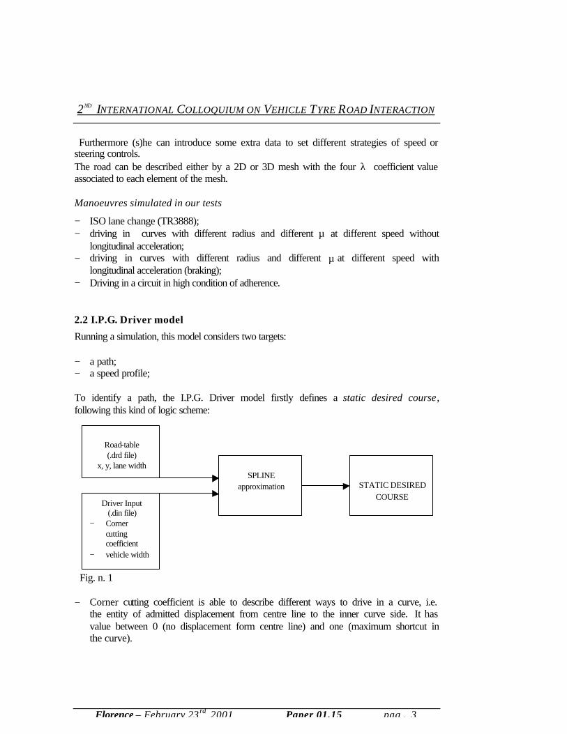
Running a simulation, this model considers two targets: − a path; − a speed profile; To identify a path, the I.P.G. Driver model firstly defines a static desired course, following this kind of logic scheme: Fig. n. 1 − Corner cutting coefficient is able to describe different ways to drive in a curve, i.e.
the entity of admitted displacement from centre line to the inner curve side. It has value between 0 (no displacement form centre line) and one (maximum shortcut in the curve).
Road-table (.drd file)
x, y, lane width
Driver Input (.din file)
− Corner cutting coefficient
− vehicle width
SPLINE
approximation
STATIC DESIRED COURSE
2ND INTERNATIONAL COLLOQUIUM ON VEHICLE TYRE ROAD INTERACTION
Florence – February 23 rd 2001 Paper 01.15 pag . 4
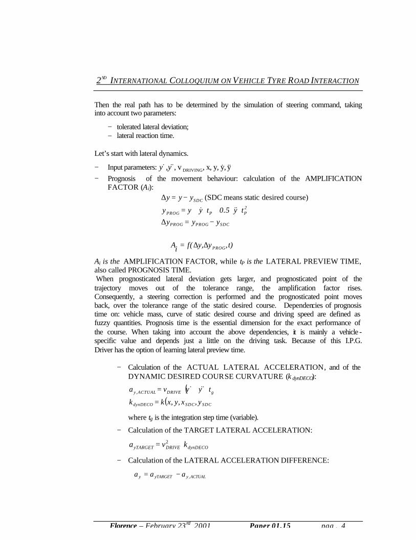
Then the real path has to be determined by the simulation of steering command, taking into account two parameters:
− tolerated lateral deviation; − lateral reaction time.
Let’s start with lateral dynamics.
− Input parameters: y ,y y,x, , v, , DRIVING &&&&&& ψψ − Prognosis of the movement behaviour: calculation of the AMPLIFICATION
FACTOR (Ai):
t) ,yy,f(iA
yyy
ty0.5tyyy
yyy
PROG
SDCPROGPROG
2PPPROG
SDC
∆∆=⇒
−=∆
⋅⋅+⋅+=
−=∆
&&&
course) desired static means (SDC
Ai is the AMPLIFICATION FACTOR, while tP is the LATERAL PREVIEW TIME, also called PROGNOSIS TIME. When prognosticated lateral deviation gets larger, and prognosticated point of the trajectory moves out of the tolerance range, the amplification factor rises. Consequently, a steering correction is performed and the prognosticated point moves back, over the tolerance range of the static desired course. Dependencies of prognosis time on: vehicle mass, curve of static desired course and driving speed are defined as fuzzy quantities. Prognosis time is the essential dimension for the exact performance of the course. When taking into account the above dependencies, it is mainly a vehicle -specific value and depends just a little on the driving task. Because of this I.P.G. Driver has the option of learning lateral preview time.
− Calculation of the ACTUAL LATERAL ACCELERATION, and of the
DYNAMIC DESIRED COURSE CURVATURE (k dynDECO):
( )( )SDCSDCdynDECO
gDRIVEACTUALy
yxyxkk
tva
,,,,
=
⋅+⋅= ψψ &&&
where tg is the integration step time (variable).
− Calculation of the TARGET LATERAL ACCELERATION:
dynDECODRIVEyTARGET kva ⋅= 2
− Calculation of the LATERAL ACCELERATION DIFFERENCE:
ACTUALyyTARGETy aaa ,−=
2ND INTERNATIONAL COLLOQUIUM ON VEHICLE TYRE ROAD INTERACTION
Florence – February 23 rd 2001 Paper 01.15 pag . 5
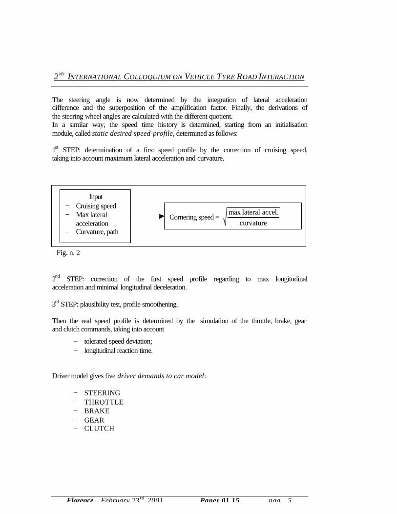
The steering angle is now determined by the integration of lateral acceleration difference and the superposition of the amplification factor. Finally, the derivations of the steering wheel angles are calculated with the different quotient. In a similar way, the speed time history is determined, starting from an initialisation module, called static desired speed-profile, determined as follows: 1st STEP: determination of a first speed profile by the correction of cruising speed, taking into account maximum lateral acceleration and curvature.
2nd STEP: correction of the first speed profile regarding to max longitudinal acceleration and minimal longitudinal deceleration. 3rd STEP: plausibility test, profile smoothening. Then the real speed profile is determined by the simulation of the throttle, brake, gear and clutch commands, taking into account
− tolerated speed deviation; − longitudinal reaction time.
Driver model gives five driver demands to car model:
− STEERING − THROTTLE − BRAKE − GEAR − CLUTCH
Input − Cruising speed − Max lateral
acceleration − Curvature, path
Cornering speed = curvature
accel. lateralmax
Fig. n. 2
2ND INTERNATIONAL COLLOQUIUM ON VEHICLE TYRE ROAD INTERACTION
Florence – February 23 rd 2001 Paper 01.15 pag . 6
2.3 Driver Lite model
Driver Lite is a sort of reduced version of I.P.G. Driver. The fundamental differences between two models can be resumed in two points. − Driver Lite is not able to LEARN, so it must obtain the best result at the first run. − Driver Lite is not able to distinguish between different lane widths, and,
consequently, it cannot introduce a corner cutting coefficient (or something similar), that seems to be an important variable to discriminate between different driving styles.
− Lateral preview time is fixed to 0.7. 2.4. Learning activity
Introducing the I.P.G. Driver functions, it is very important to describe the procedure called LEARNING, i.e. the ability of I.P.G. Driver to collect information about the vehicle, in order to use this knowledge in future simulations. By this acquired knowledge base, I.P.G. Driver can optimise the drivers’ regulation behaviour to best keep on the course. Within I.P.G. driver model the following learning activities are available:
1. BASIC_DINAMICS: driver model learns the longitudinal and lateral dynamics
2. LATERAL_DYNAMICS: driver model just learns the lateral dynamics 3. LIMIT_HANDLING: driver model aims to reach the maximum
performance. 2.4.1 The knowledge file Running a first simulation of a manoeuvre, I.P.G. Driver collects some information about the vehicle which will be taken into account in future simulations referred to the same vehicle. Selecting LIMIT_HANDLING option, I.P.G. Driver calculates the maximum speed by an iterative procedure, taking into account the maximum lateral acceleration for each value of curvature. These quantities are determined by knowing the maximum tyres slip and forces. This procedure does not require a step by step correction of lateral preview time, vehicle jaw response time and reinforcement factor steering wheel torque values. So it’s necessary only a run to have maximum speed. I.P.G. Driver learns to drive a VEHICLE, NOT to drive on a TRACK. Then if you do the learning activities in different circuits which cover a wide range of lateral acceleration and longitudinal acceleration vehicle knowledge of the driver will be quite similar in terms of: lateral preview time, vehicle jaw response time and reinforcement factor steering wheel torque values
2ND INTERNATIONAL COLLOQUIUM ON VEHICLE TYRE ROAD INTERACTION
Florence – February 23 rd 2001 Paper 01.15 pag . 7
2.4.2 Learning activity parameters
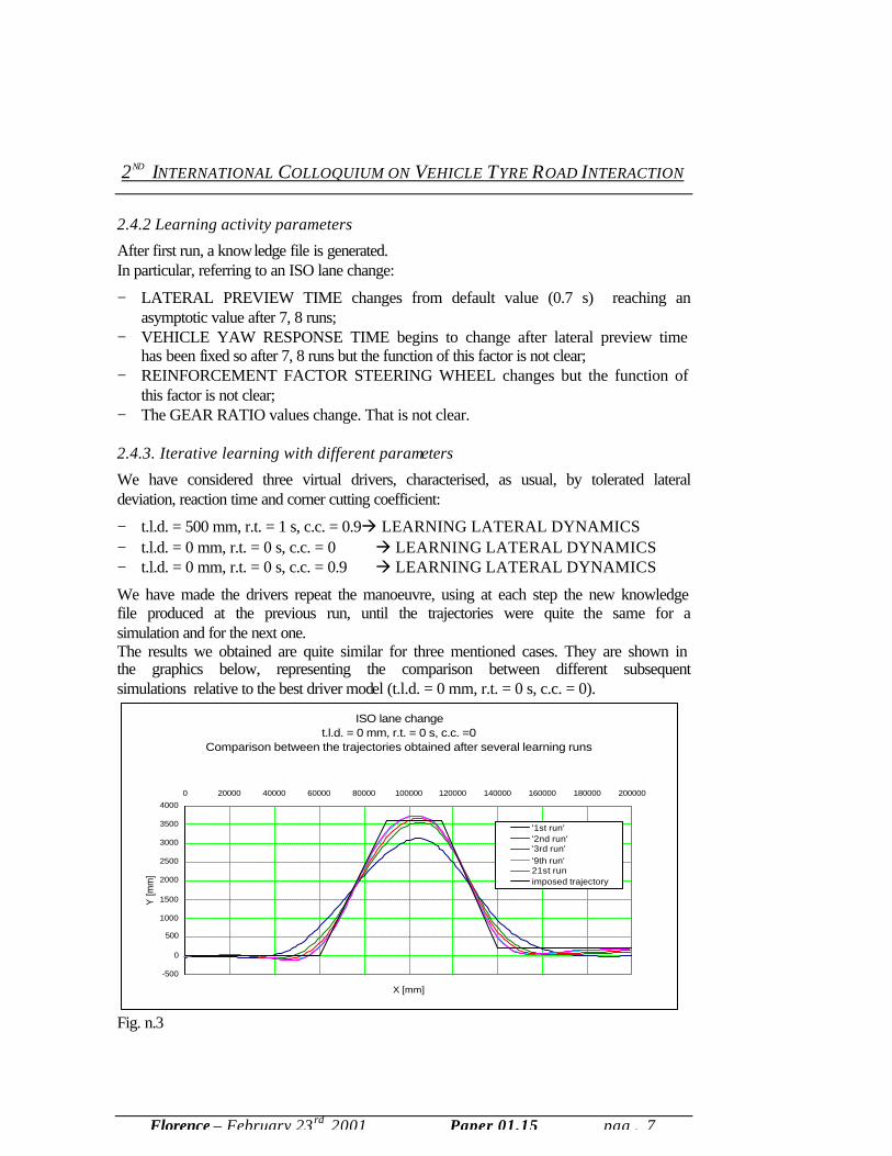
After first run, a knowledge file is generated. In particular, referring to an ISO lane change:
− LATERAL PREVIEW TIME changes from default value (0.7 s) reaching an asymptotic value after 7, 8 runs;
− VEHICLE YAW RESPONSE TIME begins to change after lateral preview time has been fixed so after 7, 8 runs but the function of this factor is not clear;
− REINFORCEMENT FACTOR STEERING WHEEL changes but the function of this factor is not clear;
− The GEAR RATIO values change. That is not clear. 2.4.3. Iterative learning with different parameters
We have considered three virtual drivers, characterised, as usual, by tolerated lateral deviation, reaction time and corner cutting coefficient:
− t.l.d. = 500 mm, r.t. = 1 s, c.c. = 0.9à LEARNING LATERAL DYNAMICS − t.l.d. = 0 mm, r.t. = 0 s, c.c. = 0 à LEARNING LATERAL DYNAMICS − t.l.d. = 0 mm, r.t. = 0 s, c.c. = 0.9 à LEARNING LATERAL DYNAMICS
We have made the drivers repeat the manoeuvre, using at each step the new knowledge file produced at the previous run, until the trajectories were quite the same for a simulation and for the next one. The results we obtained are quite similar for three mentioned cases. They are shown in the graphics below, representing the comparison between different subsequent simulations relative to the best driver model (t.l.d. = 0 mm, r.t. = 0 s, c.c. = 0).
ISO lane change t.l.d. = 0 mm, r.t. = 0 s, c.c. =0
Comparison between the trajectories obtained after several learning runs
-500
0
500
1000
1500
2000
2500
3000
3500
4000
0 20000 40000 60000 80000 100000 120000 140000 160000 180000 200000
X [mm]
Y [m
m]
'1st run''2nd run''3rd run''9th run'21st runimposed trajectory
Fig. n.3
2ND INTERNATIONAL COLLOQUIUM ON VEHICLE TYRE ROAD INTERACTION
Florence – February 23 rd 2001 Paper 01.15 pag . 8
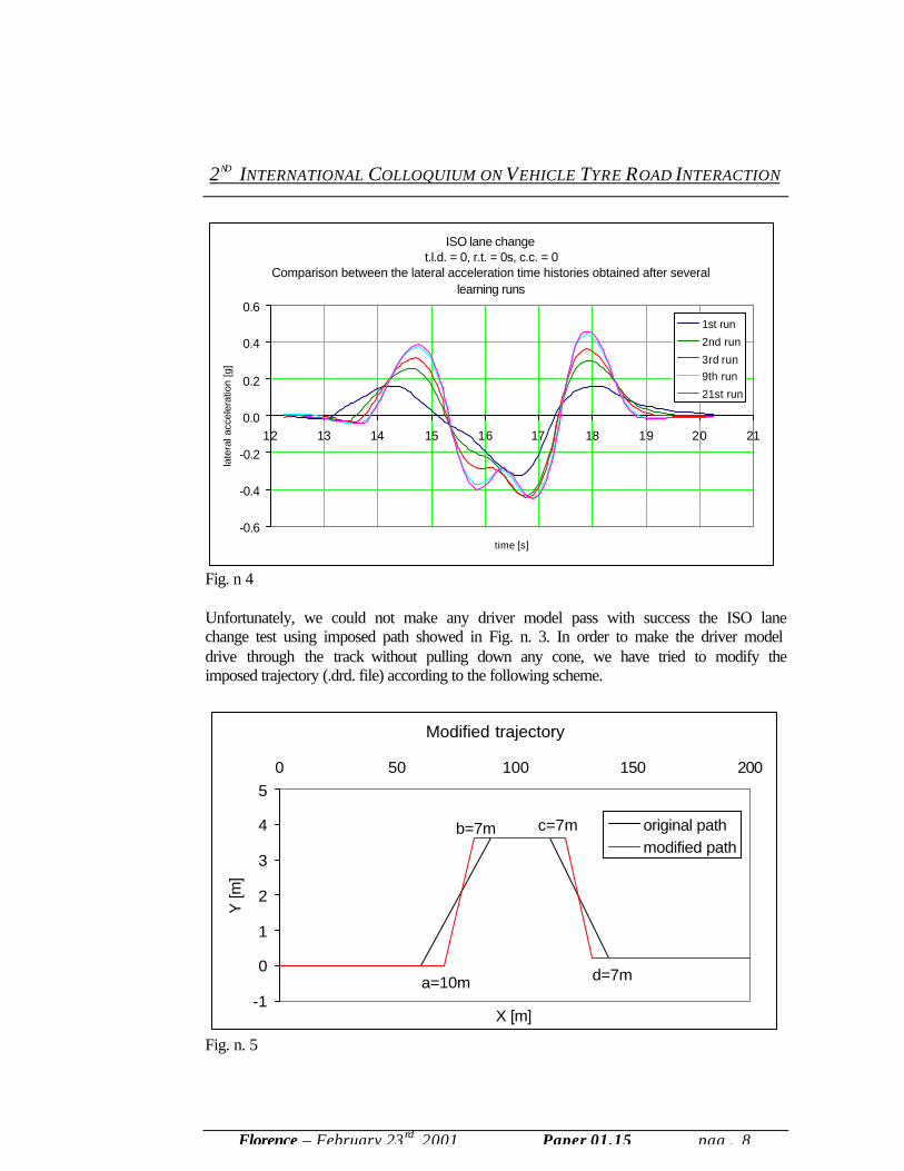
ISO lane changet.l.d. = 0, r.t. = 0s, c.c. = 0
Comparison between the lateral acceleration time histories obtained after several learning runs
-0.6
-0.4
-0.2
0.0
0.2
0.4
0.6
12 13 14 15 16 17 18 19 20 21
time [s]
late
ral a
ccel
erat
ion
[g]
1st run
2nd run
3rd run9th run
21st run
Fig. n 4 Unfortunately, we could not make any driver model pass with success the ISO lane change test using imposed path showed in Fig. n. 3. In order to make the driver model drive through the track without pulling down any cone, we have tried to modify the imposed trajectory (.drd. file) according to the following scheme.
Modified trajectory
-1
0
1
2
3
4
50 50 100 150 200
X [m]
Y [m
]
original pathmodified path
b=7m c=7m
d=7ma=10m
Fig. n. 5
2ND INTERNATIONAL COLLOQUIUM ON VEHICLE TYRE ROAD INTERACTION
Florence – February 23 rd 2001 Paper 01.15 pag . 9
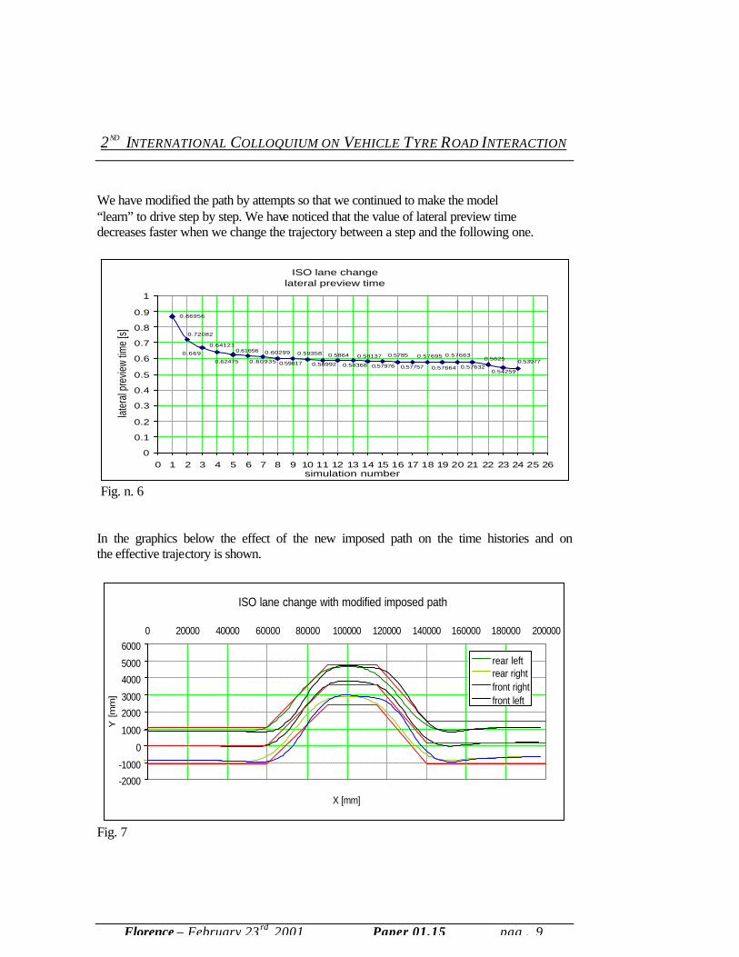
We have modified the path by attempts so that we continued to make the model “learn” to drive step by step. We have noticed that the value of lateral preview time decreases faster when we change the trajectory between a step and the following one.
ISO lane changelateral preview time
0.86956
0.53977
0.54259
0.5625
0.57632
0.57663
0.57664
0.57695
0.57757
0.5785
0.57976
0.58137
0.58368
0.5864
0.58992
0.59358
0.59817
0.60299
0.60935
0.61656
0.62475
0.64121
0.669
0.72082
0
0.1
0.2
0.3
0.4
0.5
0.6
0.7
0.8
0.9
1
0 1 2 3 4 5 6 7 8 9 10 11 12 13 14 15 16 17 18 19 20 21 22 23 24 25 26simulation number
later
al pr
eview
time
[s]
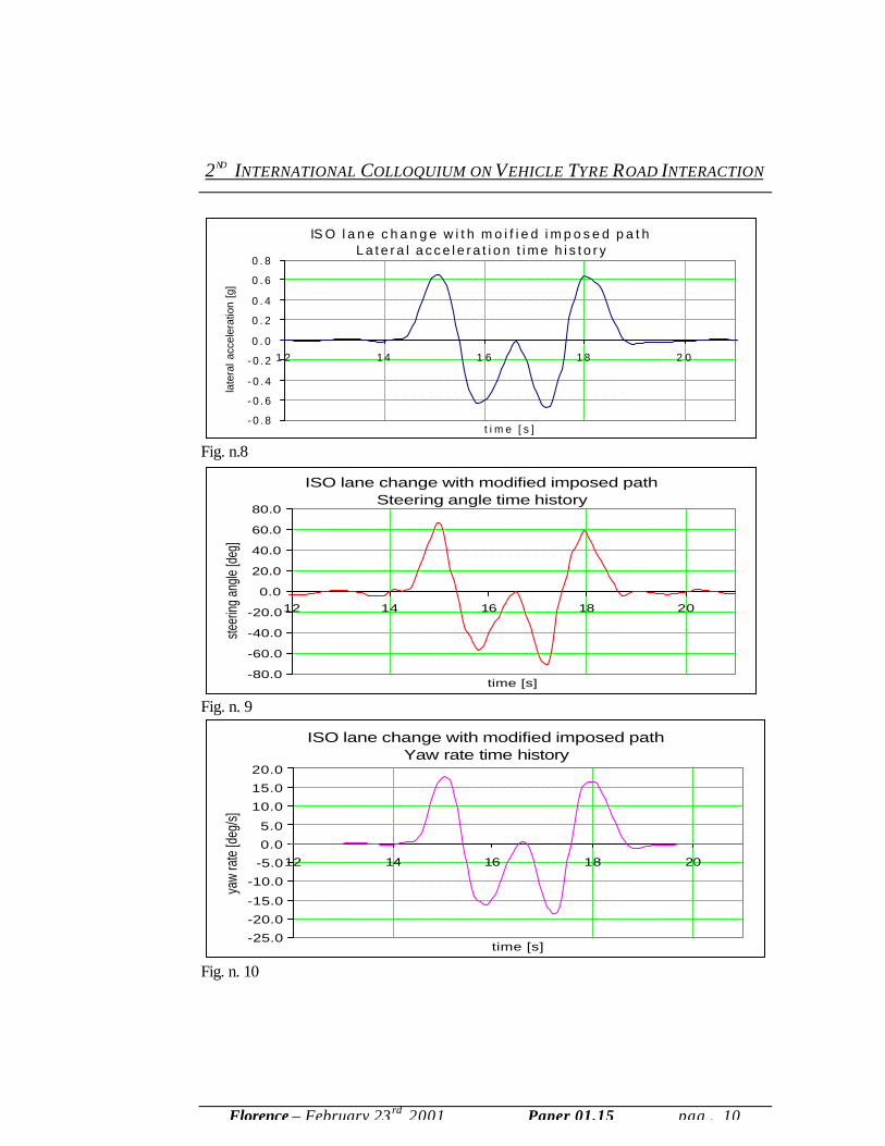
Fig. n. 6 In the graphics below the effect of the new imposed path on the time histories and on the effective trajectory is shown.
ISO lane change with modified imposed path
-2000
-1000
0
1000
2000
3000
4000
5000
60000 20000 40000 60000 80000 100000 120000 140000 160000 180000 200000
X [mm]
Y [
mm
]
rear leftrear rightfront rightfront left
Fig. 7
2ND INTERNATIONAL COLLOQUIUM ON VEHICLE TYRE ROAD INTERACTION
Florence – February 23 rd 2001 Paper 01.15 pag . 10
IS O l a n e c h a n g e w i t h m o i f i e d i m p o s e d p a t hL a t e r a l a c c e l e r a t i o n t i m e h i s t o r y
- 0 . 8
- 0 . 6
- 0 . 4
- 0 . 2
0 . 0
0 . 2
0 . 4
0 . 6
0 . 8
1 2 1 4 1 6 1 8 2 0
t i m e [ s ]
late
ral a
ccel
erat
ion
[g]
Fig. n.8
ISO lane change with modified imposed pathSteering angle time history
-80.0
-60.0
-40.0
-20.0
0.0
20.0
40.0
60.0
80.0
12 14 16 18 20
time [s]
steer
ing a
ngle
[deg
]
Fig. n. 9
ISO lane change with modified imposed pathYaw rate time history
-25.0
-20.0
-15.0
-10.0
-5.0
0.0
5.0
10.0
15.0
20.0
12 14 16 18 20
time [s]
yaw
rate
[deg
/s]
Fig. n. 10
2ND INTERNATIONAL COLLOQUIUM ON VEHICLE TYRE ROAD INTERACTION
Florence – February 23rd 2001 Paper 01.15 pag . 11
3. PARAMETRIC SIMULATIONS In order to evaluate the capability of I.P.G. Driver and Driver Lite in reproducing different manoeuvres and different drivers' behaviours, we have run some simulations aimed to answer the following questions.
− Do the results obtained in our simulations correspond to experimental ones? − Is it possible to identify different clusters of drivers, distinguishing between their
behaviour, by changing the parameters mentioned above? − Which are differences between results obtained with I.P.G. Driver and Driver Lite? − What are the most common problems that users has to face when running
simulations with I.P.G. Driver and Driver Lite? We are particularly interested in lateral dynamics; therefore, we have run our simulations trying to evaluate the effects of the parameters influencing this aspect. In this research, our achievement does not consist in reaching the best performance in terms of longitudinal speed and acceleration, but we want to investigate about models reproducing the way of following a given path, even in dangerous conditions. Using the Driver Lite, we have done parametric simulations just changing lateral preview time value. On the other hand, using I.P.G. Driver, we have considered the effects of the following parameters variation.
− corner cutting; − total lateral deviation; − lateral reaction time; − learning activity mode.
We have done parametric simulations using two different manoeuvres: − ISO lane change at different longitudinal speed (with I.P.G. and Driver Lite); − Driving in a curve using the same radius and different longitudinal speed (with
I.P.G. Driver).
The output signals we have used to evaluate the effect of parametric variations in the same manoeuvres are:
− car centre of gravity course; − lateral accelerations; − yaw rate; − side slip angle; − steering angle.
Furthermore, we have compared the r.m.s. values of steering angle and lateral acceleration obtained in our simulations with the experimental ones.
2ND INTERNATIONAL COLLOQUIUM ON VEHICLE TYRE ROAD INTERACTION
Florence – February 23 rd 2001 Paper 01.15 pag . 12
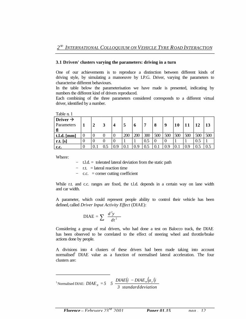
3.1 Drivers' clusters varying the parameters: driving in a turn One of our achievements is to reproduce a distinction between different kinds of driving style, by simulating a manoeuvre by I.P.G. Driver, varying the parameters to characterise different behaviours. In the table below the parameterisation we have made is presented, indicating by numbers the different kind of drivers reproduced. Each combining of the three parameters considered corresponds to a different virtual driver, identified by a number. Table n. 1 Driver à Parameters ↓
1 2 3 4 5 6 7 8 9 10 11 12 13
t.l.d. [mm] 0 0 0 0 200 200 300 500 500 500 500 500 500 r.t. [s] 0 0 0 0 1 1 0.5 0 0 1 1 0.5 1 c.c. 0 0.1 0.5 0.9 0.1 0.9 0.5 0.1 0.9 0.1 0.9 0.5 0.5 Where:
− t.l.d. = tolerated lateral deviation from the static path − r.t. = lateral reaction time − c.c. = corner cutting coefficient
While r.t. and c.c. ranges are fixed, the t.l.d. depends in a certain way on lane width and car width. A parameter, which could represent people ability to control their vehicle has been defined, called Driver Input Activity Effect (DIAE):
∑
= 2
2
DIAEdt
d ψ
Considering a group of real drivers, who had done a test on Balocco track, the DIAE has been observed to be correlated to the effect of steering wheel and throttle/brake actions done by people. A divisions into 4 clusters of these drivers had been made taking into account normalised1 DIAE value as a function of normalised lateral acceleration. The four clusters are:
1 Normalised DIAE: ( ) ( )( )
deviation standard3
iaDIAEiDIAE55DIAE ym
N ⋅
−⋅+=
2ND INTERNATIONAL COLLOQUIUM ON VEHICLE TYRE ROAD INTERACTION
Florence – February 23rd 2001 Paper 01.15 pag . 13
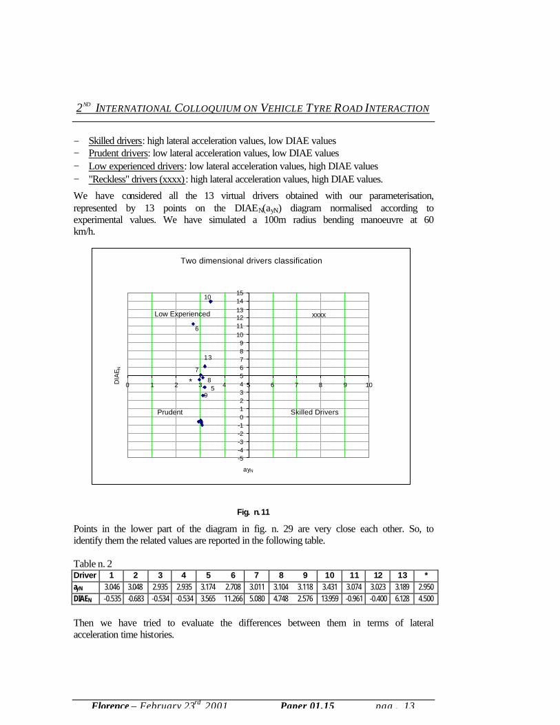
− Skilled drivers: high lateral acceleration values, low DIAE values − Prudent drivers: low lateral acceleration values, low DIAE values − Low experienced drivers: low lateral acceleration values, high DIAE values − "Reckless" drivers (xxxx): high lateral acceleration values, high DIAE values.
We have considered all the 13 virtual drivers obtained with our parameterisation, represented by 13 points on the DIAEN(ayN) diagram normalised according to experimental values. We have simulated a 100m radius bending manoeuvre at 60 km/h.
Two dimensional drivers classification
-5-4-3-2-10123456789
101112131415
0 1 2 3 4 5 6 7 8 9 10
ayN
DIA
E N
Low Experienced
Prudent
5
6
7
9
10
13
* 8
xxxx
Skilled Drivers
Fig. n.11
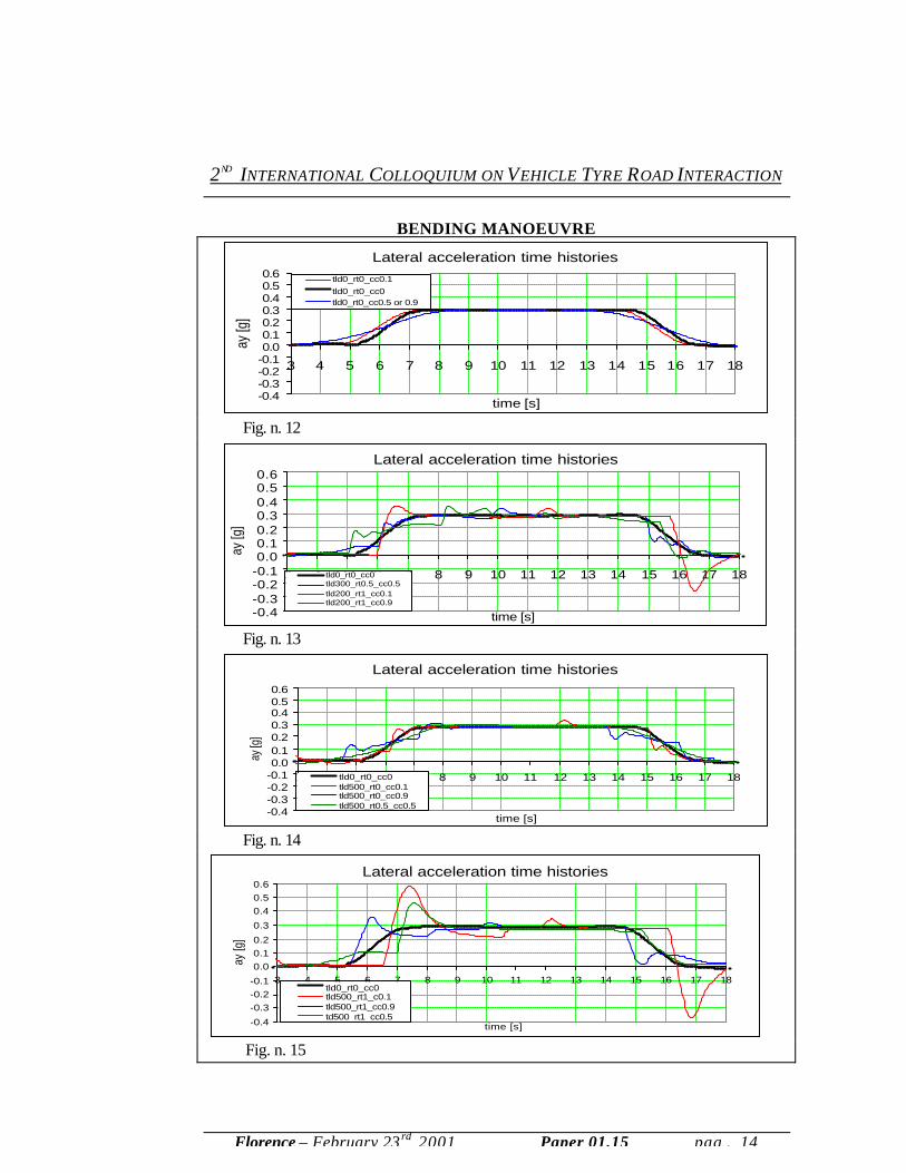
Points in the lower part of the diagram in fig. n. 29 are very close each other. So, to identify them the related values are reported in the following table. Table n. 2 Driver 1 2 3 4 5 6 7 8 9 10 11 12 13 * ayN 3.046 3.048 2.935 2.935 3.174 2.708 3.011 3.104 3.118 3.431 3.074 3.023 3.189 2.950 DIAEN -0.535 -0.683 -0.534 -0.534 3.565 11.266 5.080 4.748 2.576 13.959 -0.961 -0.400 6.128 4.500 Then we have tried to evaluate the differences between them in terms of lateral acceleration time histories.
2ND INTERNATIONAL COLLOQUIUM ON VEHICLE TYRE ROAD INTERACTION
Florence – February 23 rd 2001 Paper 01.15 pag . 14
BENDING MANOEUVRE
Lateral acceleration time histories
-0.4-0.3-0.2-0.10.00.10.20.30.40.50.6
3 4 5 6 7 8 9 10 11 12 13 14 15 16 17 18
time [s]
ay [g
]
tld0_rt0_cc0.1tld0_rt0_cc0tld0_rt0_cc0.5 or 0.9
Fig. n. 12
Lateral acceleration time histories
-0.4-0.3-0.2-0.10.00.10.20.30.40.50.6
3 4 5 6 7 8 9 10 11 12 13 14 15 16 17 18
time [s]
ay [g
]
tld0_rt0_cc0tld300_rt0.5_cc0.5tld200_rt1_cc0.1tld200_rt1_cc0.9
Fig. n. 13
Lateral acceleration time histories
-0.4-0.3-0.2-0.10.00.10.20.30.40.50.6
3 4 5 6 7 8 9 10 11 12 13 14 15 16 17 18
time [s]
ay [g
]
tld0_rt0_cc0tld500_rt0_cc0.1tld500_rt0_cc0.9tld500_rt0.5_cc0.5
Fig. n. 14
Lateral acceleration time histories
-0.4
-0.3-0.2-0.1
0.00.10.2
0.3
0.40.50.6
3 4 5 6 7 8 9 10 11 12 13 14 15 16 17 18
time [s]
ay [g
]
tld0_rt0_cc0tld500_rt1_c0.1tld500_rt1_cc0.9td500_rt1_cc0.5
Fig. n. 15
2ND INTERNATIONAL COLLOQUIUM ON VEHICLE TYRE ROAD INTERACTION
Florence – February 23rd 2001 Paper 01.15 pag . 15
How the three parameters influence the driver behaviour? − An increasing t.l.d. reproduces the behaviour of a driver who is not able to
correctly follow the trajectory. In fact a deviation of static path generates an irregular real path. So corresponding lateral acceleration and steering angle time histories are characterised by a great number of peaks.
− Reaction time amplifies the effect described above. The model corrects its trajectory when it realises that tolerated limit is exceeded. If reaction time increases, it takes a longer time for the model to do something about this situation. So the behaviour reproduced corresponds to a slowly reacting driver.
− A high corner cutting coefficient value makes the static path smoother. So the corresponding driver reaches lower lateral acceleration values being equal the other parameters. It does not necessarily correspond to the behaviour of a skilled driver, who is able to drive very close to the imposed path, reaching high lateral accelerations, but with low DIAE, it reproduces a prudent driver.
− Sometimes one effect can balance another one. Looking at drivers 12 and 2 we can observe that they are very closed each other, even if they correspond to very different values of the three parameters. Driver 12 balances the high values of t.l.d. and r.t. with a c.c. equal to 0.5.
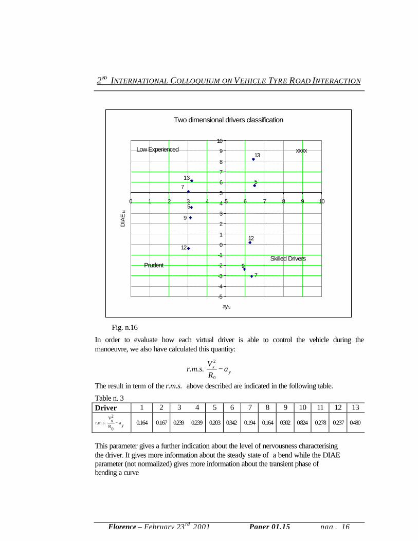
Note that this parameterisation is just referred to the part of the track where lateral acceleration is bigger than 2 m/s2. Looking at the diagram representing normalised DIAE as a function of normalised lateral acceleration, we can immediately notice that the points referring to different drivers are in a very small lateral acceleration range. This is due to the constant values of radius and longitudinal speed in our simulations. The point “*” corresponds to a simulation run with the knowledge file obtained after 20 runs of ISO lane change and with the same .din file identifying the virtual driver n.2. Considering some of the points corresponding to different drivers, we have tried to determine the related ones increasing the longitudinal speed up to 80 km/h. As shown in the graphic in fig. n. 16, the stratification between the different drivers behaviours does not remain. In fact some of them increase their value increasing the speed and some decrease. Trying to reproduce a large number of points, covering a big area on the considered diagram, it is necessary to make the model perform the manoeuvre at different imposed velocities.
In order to evaluate how each virtual driver is able to control the vehicle during the manoeuvre, we also have calculated this quantity:
− y
x aRV
r.m.s.0
2
2ND INTERNATIONAL COLLOQUIUM ON VEHICLE TYRE ROAD INTERACTION
Florence – February 23 rd 2001 Paper 01.15 pag . 16
Two dimensional drivers classification
-5
-4
-3
-2
-1
0
1
2
3
4
5
6
7
8
9
10
0 1 2 3 4 5 6 7 8 9 10
ayN
DIA
EN
Low Experienced
PrudentSkilled Drivers
xxxx
5
5
9
9
7
7
12
12
13
13
Fig. n.16
In order to evaluate how each virtual driver is able to control the vehicle during the manoeuvre, we also have calculated this quantity:
− y
x aRV
r.m.s.0
2
The result in term of the r.m.s. above described are indicated in the following table.
Table n. 3 Driver 1 2 3 4 5 6 7 8 9 10 11 12 13
− ya
0R
2xV
r.m.s.
0.164 0.167 0.239 0.239 0.203 0.342 0.194 0.164 0.302 0.824 0.278 0.237 0.480
This parameter gives a further indication about the level of nervousness characterising the driver. It gives more information about the steady state of a bend while the DIAE parameter (not normalized) gives more information about the transient phase of bending a curve
2ND INTERNATIONAL COLLOQUIUM ON VEHICLE TYRE ROAD INTERACTION
Florence – February 23rd 2001 Paper 01.15 pag . 17
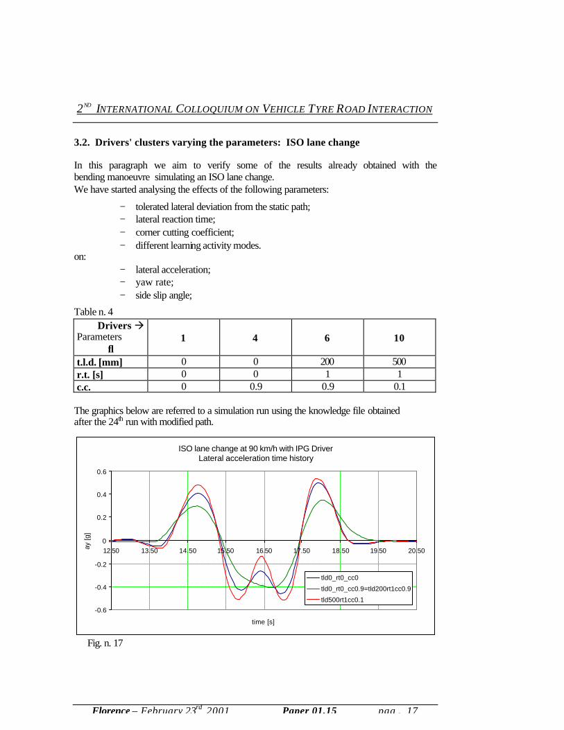
3.2. Drivers' clusters varying the parameters: ISO lane change In this paragraph we aim to verify some of the results already obtained with the bending manoeuvre simulating an ISO lane change. We have started analysing the effects of the following parameters:
− tolerated lateral deviation from the static path; − lateral reaction time; − corner cutting coefficient; − different learning activity modes.
on: − lateral acceleration; − yaw rate; − side slip angle;
Table n. 4 Drivers à
Parameters ↓
1 4 6 10
t.l.d. [mm] 0 0 200 500 r.t. [s] 0 0 1 1 c.c. 0 0.9 0.9 0.1
The graphics below are referred to a simulation run using the knowledge file obtained after the 24th run with modified path.
ISO lane change at 90 km/h with IPG DriverLateral acceleration time history
-0.6
-0.4
-0.2
0
0.2
0.4
0.6
12.50 13.50 14.50 15.50 16.50 17.50 18.50 19.50 20.50
time [s]
ay [g
]
tld0_rt0_cc0
tld0_rt0_cc0.9=tld200rt1cc0.9
tld500rt1cc0.1
Fig. n. 17
2ND INTERNATIONAL COLLOQUIUM ON VEHICLE TYRE ROAD INTERACTION
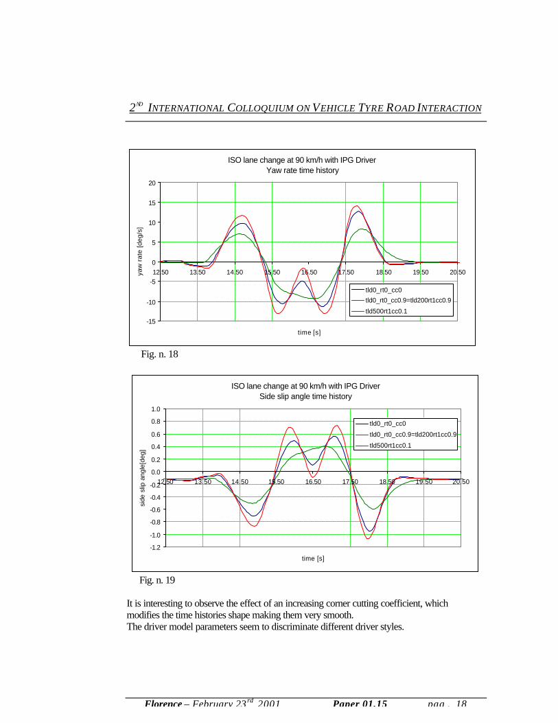
Florence – February 23 rd 2001 Paper 01.15 pag . 18
ISO lane change at 90 km/h with IPG DriverYaw rate time history
-15
-10
-5
0
5
10
15
20
12.50 13.50 14.50 15.50 16.50 17.50 18.50 19.50 20.50
time [s]
yaw
rat
e [d
eg/s
]
tld0_rt0_cc0
tld0_rt0_cc0.9=tld200rt1cc0.9
tld500rt1cc0.1
Fig. n. 18
ISO lane change at 90 km/h with IPG DriverSide slip angle time history
-1.2
-1.0
-0.8
-0.6
-0.4
-0.2
0.0
0.2
0.4
0.6
0.8
1.0
12.50 13.50 14.50 15.50 16.50 17.50 18.50 19.50 20.50
time [s]
side
slip
ang
le[d
eg]
tld0_rt0_cc0
tld0_rt0_cc0.9=tld200rt1cc0.9
tld500rt1cc0.1
Fig. n. 19 It is interesting to observe the effect of an increasing corner cutting coefficient, which modifies the time histories shape making them very smooth. The driver model parameters seem to discriminate different driver styles.
2ND INTERNATIONAL COLLOQUIUM ON VEHICLE TYRE ROAD INTERACTION
Florence – February 23rd 2001 Paper 01.15 pag . 19
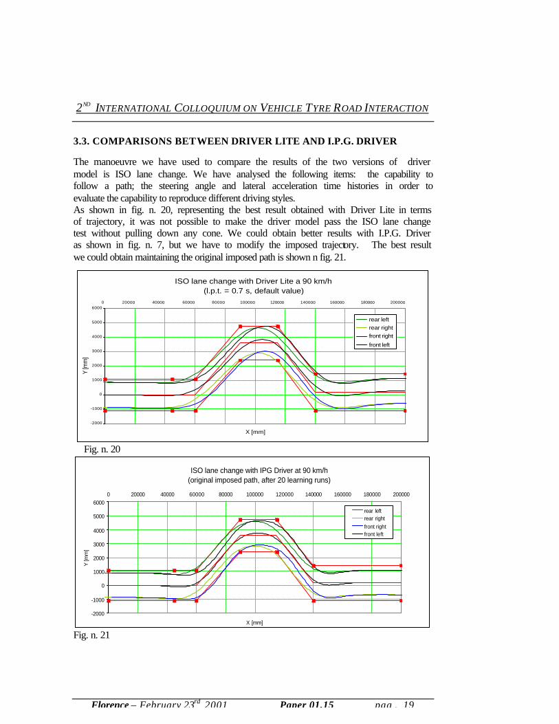
3.3. COMPARISONS BETWEEN DRIVER LITE AND I.P.G. DRIVER
The manoeuvre we have used to compare the results of the two versions of driver model is ISO lane change. We have analysed the following items: the capability to follow a path; the steering angle and lateral acceleration time histories in order to evaluate the capability to reproduce different driving styles. As shown in fig. n. 20, representing the best result obtained with Driver Lite in terms of trajectory, it was not possible to make the driver model pass the ISO lane change test without pulling down any cone. We could obtain better results with I.P.G. Driver as shown in fig. n. 7, but we have to modify the imposed trajectory. The best result we could obtain maintaining the original imposed path is shown n fig. 21.
ISO lane change with Driver Lite a 90 km/h (l.p.t. = 0.7 s, default value)
-2000
-1000
0
1000
2000
3000
4000
5000
60000 20000 40000 60000 80000 100000 120000 140000 160000 180000 200000
X [mm]
Y [m
m]
rear leftrear rightfront right
front left
Fig. n. 20
ISO lane change with IPG Driver at 90 km/h(original imposed path, after 20 learning runs)
-2000
-1000
0
1000
2000
3000
4000
5000
60000 20000 40000 60000 80000 100000 120000 140000 160000 180000 200000
X [mm]
Y [m
m]
rear leftrear rightfront rightfront left
Fig. n. 21
2ND INTERNATIONAL COLLOQUIUM ON VEHICLE TYRE ROAD INTERACTION
Florence – February 23 rd 2001 Paper 01.15 pag . 20
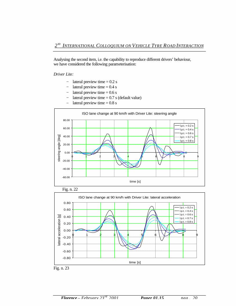
Analysing the second item, i.e. the capability to reproduce different drivers’ behaviour, we have considered the following parameterisation: Driver Lite:
− lateral preview time = 0.2 s − lateral preview time = 0.4 s − lateral preview time = 0.6 s − lateral preview time = 0.7 s (default value) − lateral preview time = 0.8 s
ISO lane change at 90 km/h with Driver Lite: steering angle
-60.00
-40.00
-20.00
0.00
20.00
40.00
60.00
80.00
0 1 2 3 4 5 6 7 8 9
time [s]
stee
ring
angl
e [d
eg]
l.p.t. = 0.2 sl.p.t. = 0.4 sl.p.t. = 0.6 sl.p.t. = 0.7 sl.p.t. = 0.8 s
Fig. n. 22
ISO lane change at 90 km/h with Driver Lite: lateral acceleration
-0.80
-0.60
-0.40
-0.20
0.00
0.20
0.40
0.60
0.80
0 1 2 3 4 5 6 7 8 9
time [s]
late
ral a
ccel
erat
ion
[g]
l.p.t. = 0.2 sl.p.t. = 0.4 sl.p.t. = 0.6 s
l.p.t. = 0.7 sl.p.t. = 0.8 s
Fig. n. 23
2ND INTERNATIONAL COLLOQUIUM ON VEHICLE TYRE ROAD INTERACTION
Florence – February 23rd 2001 Paper 01.15 pag . 21
With Driver Lite we have to impose a very low value of preview time to make the model produce time histories similar to the experimental ones (with the characteristic maximum point in the middle of central corridor). This low value of lateral preview time can give a lot of stability problems to the control. In this case the problem is evident at the end of iso lane change simulation with high signal oscillations. On the other hand I.P.G. Driver gives better results, but it takes a long time because of the high number of simulation needed. 3.4. Comparison between the results of our simulations and the experimental ones
We aimed to compare the results obtained in ISO lane change simulations with the experimental values. We have considered some simulations run with the I.P.G. Driver and we have calculated the r.m.s. values of the lateral acceleration and steering angle time histories, taking into account just the part of track corresponding to the “real” ISO lane change, cutting the extra straight parts at the beginning and at the end of the track. The results presented below are referred to the simulation run at the 24th learning step with modified imposed path.
deg 28.696angle) steering.(s.m.r
g 328.0)a.(s.m.r y
=
=
They are quite similar to the experimental ones.
2ND INTERNATIONAL COLLOQUIUM ON VEHICLE TYRE ROAD INTERACTION
Florence – February 23 rd 2001 Paper 01.15 pag . 22
3. CONCLUSION
Driver behaviour introduces a new set of variables when you evaluate vehicle behaviour in closed loop manoeuvres. We tried to understand the capability of I.P.G. Driver to do closed loop manoeuvres and its capability to discriminate different drivers with simple parameters. The target is to understand how driver change vehicle behaviour in closed loop manoeuvres in order to read them without considering driver style. We found that: − I.P.G. Driver permits to simulate manoeuvres with different driving styles varying
some input parameters. − There’s a good correspondence between its results and experimental tests, where
different driver styles had been defined through simple parameters. In case of a curve:
∑
= 2
2
DIAEdt
d ψ for transient phase;
− y
x aRVr.m.s.
0
2
for steady phase.
− It is very difficult to simulate an ISO lane change without pulling down any cone
with I.P.G. Driver using the standard path: we had to modify the imposed path and to run a very high number of learning simulations to obtain good results.
− It’s important to make fine tuning of the desired path in order to have success in simulations.
− The kind of learning activity has a relevant influence on the driver reproduced by the model, balancing for instance the lack of readiness or improving the lane-keeping capability.
− The way that I.P.G. Driver changes some parameters, it’s not clear. − It needs a lot of time to do parameter set up and run simulation in order to reach
good result . − It’s possible to define simple parameters which differentiate driver style. − I.P.G. Driver model is not an user friendly product.
2ND INTERNATIONAL COLLOQUIUM ON VEHICLE TYRE ROAD INTERACTION
Florence – February 23rd 2001 Paper 01.15 pag . 23
ACKNOWLEDGMENTS
The author wishes to acknowledge all the partners of the VERT Project, funded by the European Commission. CONTACT
Leonardo Pascali Dr. Ing. Centro Ricerche FIAT Strada Torino, 50 I-10043 Orbassano (Torino)
REFERENCES
1. Kondo, M. et al. ‘Driver’s sight point and dynamics of-driver vehicle system realted to it’, SAE paper 680104 (1968).
2. M.Mitschke, A. Apel ‘Driver behaviour model for longitudinal and directional control in emergency manoeuvres’, EAEC 5th International Congress Strasbourg, 21-23 June (1995).
3. A. Apel and M. Mitschke ‘Adjusting vehicle characteristics by means of driver models’, Int. J. of vehicle design, Vol. 18, No.6, pp.583-596 (1997).
4. Mouri, H., Furusho, H., ‘Investigation of automatic path tracking –Comparing the performance of LQ control with that of PD control’, Trans. JSAE, Vol.30, No. 1, pp. 121-126 (1999).
5. Mouri, H.,Yoshitaka Marumo, ‘Study on automatic path track using virtual point regulator’, Trans. JSAE, Vol.21, pp. 523-528 (2000).
6. ‘A Mathematical Model for Driver steering Control, with Design, Tuning and Performance Results’, V.S.D., Vol. 33, pp.289-326 (2000).
7. ISO/DIS 3888 Passenger cars – Test track for a severe lane-change manoeuvre