AD-A 197 2*4RADC-.TR-s-44Final Technical ReportApril 1988

Ii

:I

EUCLIDEAN DECODERS FOR BCHCODES

1

The MITRE Corporation

Wil~ard L. Eastman

z

i I :

= APPROVED FOR PUBLIC RELEASE; DISTRISUTION UNLIIW TED. :I DTIC-mELECTE

*1 JUL 0 8 1988

i ROME AIR DEVELOPMENT CENTERAir Force Systems Command

Griffiss Air Force Base, NY 13441-5700,!

i "'

A BEST 08 033AVAILABLE COPY

_46 Vrep.~ni' bawa reviwed by the RAZ)C Public Affairs office (PA) and* ~ W"*tble to tba htional techeical tnforuation Service (NTIS). At NTIS

*iU WJ be rolsa"ble to. the iseralr public,. including foreign nations.

T"9644 bas' bee reviewed and is approved for publication.

JOHN J. PATTIProjeact Engineer

7,'

tifg Teehnical DirectorDirectorate of Coimmunicatious.

FOR THlE COMNADER:

JAMES W. HYDE, IIIDirectorate of Plans-& Program

If your address has changed. or if you wish to be removed from the RADC

mnaitlng list, or if the addressee is no longer employed by your organization,plesee notify RADC (DCCD) Griffiss APE NY 13441-5700. This will assist us inmaintaining a current mailing list.

Do not return copies of this report unless contractual obligations ornoties. on a specific document require that it be returned.

V

UNCLASSIFIED

SECURITY CLASSIFICATION OF THIS PAGE

REPORT DOCUMENTATION PAGE oAINo 07p o0v88

Is. REPORT SECURITY CLASSIFICATION lb. RESTRICTIVE MARKINGS

UNCLASSIFIED N/A2a. SECURITY CLASSIFICATION AUTHORITY 3. DISTRIBUTION/AVAILABILITY OF REPORTN/A Approved for public release;

2b. DECLASSIFICATION /DOWNGRADING SCHEDULE distribution unlimited

N/A4. PERFORMING ORGANIZATION REPORT NUMBER(S) S. MONITORING ORGANIZATION REPORT NUMBER(S)

MTR10197 RADC-TR-88-44

NI. NAME OF PERFORMING ORGANIZATION 6b. OFFICE SYMBOL 7a. NAME OF MONITORING ORGANIZATIONThe MITRE Corporation licable)

D82 Rome Air Development Center (DCCD) ,

6C. ADDRESS (C1y, State, end ZIP Code) 7b. ADDRESS (Cty, State, and ZIP Code)D82-L-22

Burlington Road Griffiss AFB NY 13441-5700Bedford HA 01730

$. NAME OF FUNDING/SPONSORING 6b. OFFICE SYMBOL 9 PROCUREMENT INSTRUMENT IDENTIFICATION NUMBERORGANIZATION (f applicable)

Rome Air Development Center DCCD F19628-86-C-0001

fc. ADDRESS (City, State, and ZIP Code) 10. SOURCE OF FUNDING NUMBERSPROGRAM PROJECT TASK WORK UNIT 0

Griffiss AFB NY 13441-5700 ELEMENT NO. NO. NO CCSSION NO._______________MOLE 75 60,"

11. TITLE (Include Security Classification)

EUCLIDEAN DECODERS FOR BCH CODES

12. PERSONAL AUTHOR(S)

W1llArd L. Eastman13a. TYPE OF REPORT 13b. TIME COVERED 14. DATE OF REPORT (Year, Month, Day) 15. PAGE COUNT

Final FROM TO _0"_86 April 1988 19416. SUPPLEMENTARY NOTATION /

N/A

17. COSATI CODES 1,210. SUBJECT TERMS (Continue on reverse If necemsay and dentify by block number)FIELD GROUP SUB-GROUP Communications

25 02 Coding;25 05 Error Correction Codes ( !

19. ABSTRACT (Continue on reveuse if necessary and ident/ by block number) 1 V6This report investigates conventional decoding algorithms for BCH codes. The algorithm ofSugiyama, Kasahara, Hirasawa and Namekawa, Mills' continued fraction algorithm, and theBerlekamp-Massey algorithm are all viewed as slightly differing variants of Euclid'salgorithm. An improved version of Euclid's algorithm for polynomials is developed. TheBerlekamp-Massey algorithm is extended within the Euclidean framework to avoid computationof vector inner products. Inversionless forms of the algorithms are considered and the

results are extended to provide for decoding of erasures a well as errors. .

20. DISTRIBUTION/AVAILABILITY OF ABSTRACT 21. ABSTRACT SECURITY CLASSIFICATION ' 'r.OUNCLASSIFIED/UNLIMITED 3 SAME AS RPT. Q DTIC USERS UNCLASSIFIED

22a. NAME OF RESPONSIBLE INDIVIDUAL 22b. TELEPHONE (Include Area Code) 22c. OFFICE SYMBOL

-John J. Patti 315 330-3224 T RADC (DCCD)DO Form 1473, JUN 86 Pre vious ed itons are obsolete. SECURITY CLASSIFICATION OF THIS PAGE

UNCLASSIFIED

XECUTIVE SUMMARY

This report examines and evaluates three leading conventional

decoding algorithms for BCH and Reed-Solomon error-correcting codes:

* the decoding algorithm of Sugiyama et al., which is based on

Euclid's algorithm 0

* a decoding algorithm developed by Scholtz and Welch based on

Mills' continued fraction expansion

e the Berlekamp-Massey decoding algorithm.

The three algorithms can be viewed as slightly differing variations

of Euclid's algorithm for finding the greatest common divisor of two

polynomials. All, in appropriate versions, are suitable for VLSI

implementation in a two-dimensional array for pipelined decoding of

received codeword polynomials distorted by errors and erasures.

Extension of the classical decoding theory for BCH codes 6

The classical decoding theory for t-error-correcting BCH codes

as developed by Peterson, Gorenstein and Zierler, Chien, Forney, and

Berlekamp is centered about the key equation

Acce !ion For

Q(x) = S(x)k(x) (mod x2t) NTIS GF,,

F v-,I l " 'it, o eiJL t c

-0,-- .; . ' or 1

N% .r N..rPp

%s~i Z.'.y5 %~ % % .,%

. ,," -l%

relating three important polynomials:

* the known syndrome polynomial S(x)

* the unknown error locator polynomial k(x)

* the unknown error evaluator polynomial n(x)

The three conventional algorithms under study solve this

equation for the unknown polynomials &(x) and (x) given the known

syndrome polynomial S(x). The error locations can then be

determined by a Chien search for the zeros of A(x) and the error

magnitudes can be calculated directly by Forney's formula

y-1AQ(X.

where Yj is the jth error magnitude, Xj is the field element

denoting the jth error location, and k'(x) is the formal derivative

of the error locator polynomial.

We have rounded out the classical theory by defining a new

polynomial 4(x) such that

&(x)S(x) = x2tR.(x) + O(x).

The polynomial A(x) contains the same information as the

error evaluator polynomial O() in that the syndrome polynomial can

be recovered either from the pair (Q(x), A(x)) or from the pair

W.

Io

(A(x), A(x)). This leads to the derivation of a new formula for

calculation of the error magnitudes in terms of A(x) and &(x). This

new formula (an alternative to Forney's formula) can be used if A(x)

is easier to calculate than Q(x).

Inside Euclid's algorithm

O

Euclid's famous algorithm for finding the greatest common

divisor of two integers can be immediately generalized for finding

the greatest common divisior of two polynomials f(x) and g(x) over a

given field. In the extended version, the algorithm also yieldsO

polynomials a(x) and b(x) satisfying

gcd(f(x), g(x)) = a(x)f(x) + b(x)g(x).

0This form of the algorithm, with suitable modifications, can be used

to solve the key equation to produce the error locator polynomial

A(x) and the error evaluator polynomial Q(x) (or scalar multiples

yA(x) and yo(x) for some field element y), given the syndrome

polynomial S(x). Euclid's algorithm is the basis both for the

decoding algorithm of Sugiyama, et. al. and for the decoding

algorithm based on Mills' continued fraction expansion.

Imbedded within Euclid's algorithm is a polynomial division,

itself an iterative process, which must be performed once during

each iteration of the algorithm. To implement the algorithm in a

systolic array, it is desirable to break the polynomial division

down into its component sequence of partial divisions, where each

partial division consists of a field element inversion, a

multiplication of a polynomial by a scalar, and a polynomial

subtraction.

v.V. % %X% %% % %%"

NI XVI W .n.._k11W

We have looked inside Euclid's algorithm to examine the

implications of this replacement. When the polynomial divisions are

replaced by a sequence of partial divisions, Euclid's algorithm

exhibits a two-loop structure; one loop is executed when the partial

division does not complete a polynomial division, and the other loop

is executed whenever the partial division does complete the

polynomial division. (Both loops contain common steps.) A valid,

cleaner, and more efficient algorithm can be obtained by deleting

one of the loops, with suitable modifications to the remaining

loop. The resulting improved algorithm bears a striking resemblance

to Berlekamp's algorithm. In effect, this study shows why the

Berlekamp-Nassey decoding algorithm is more efficient than the

decoding algorithms based directly on Euclid's algorithm.

The Berlekamp-Massey algorithm in a Euclidean context 0

Both the Berlekamp-Massey algorithm and the decoding algorithmsbased upon Euclid's algorithm can be improved by adopting features

from each other. The chief drawback of the Berlekamp-Massey

algorithm when implementated in a systolic array is the need to

calculate a discrepancy between the value of the next syndrome

symbol and the next symbol output by the current linear feedbackshift register (in Massey's formulation). This calculation requires

an inner-product computation at each iteration of the algorithm, a

computation whose length increases with the number of iterations.

We have expanded the Berlekamp-Massey algorithm, employing

additional polynomials including a remainder-like polynomial r(x)

that corresponds to the remainder polynomial retained in the

Euclidean decoding algorithms. Retention of r(x) obviates the need

to calculate the discrepancy at each iteration, for at itcration j

the jth discrepancy is given by the coefficient rj. Thus, at the

vi

%.iv %,OI I .... _.E.],j- w- . w-, , , '. , ',Z' - - '," .,, ",.,..... ,.... ".- #; Zg, . , %-, . ,%

cost of additional multiplications and storage, expansion of the

Berlekamp-riassey algorithm in a Euclidean context renders the

algorithm suitable for VLSI implementation in a two-dimensional

systolic array.

The Mills'algorithm in a Berlekamp-Massey context

Similarly, the decoding algorithms based on Euclid's algorithm

can be improved by modifications that move them closer to

Berlekamp's algorithm. The polynomial divisions in Mills' decoding

algorithm are replaced by a sequence of partial divisions, again

resulting in a two-loop structure. One loop is then removed, n

yielding an improved decoding algorithm based on our enhanced

version of Euclid's algorithm. We have confirmed the validity of

the new algorithm by demonstrating that the partial results

generated by the algorithm can be mapped by scalar multiplication

into partial results generated by its predecessor. The new version

of the Mills' algorithm closely resembles the Euclideanized version

of the Berlekamp-Massey algorithm, and scalar multiples of the

partial results obtained from the one are equated to the partial

results obtained from the other. This demonstrates an equivalence

among all three of the decoding algorithms studied.

Inversionless decoding algorithms .

The three decoding algorithms under study and the variants and..-

hybrid versions constructed therefrom all require finite field

divisions or, equivalently, inversion of finite field elements.

These requirements can be removed, at the cost of further scalar"- ,

multiplications, by Burton's technique. When Burton's X.O.

transformation is applied to the Euclideanized Berlekamp-Massey

vii

A, eo.A

S

algorithm and to the enhanced version of the Mills algorithm, the P

resulting algorithms are identical, except for an algebraic sign in

one step.

Decoding with erasures ./ .

Forney has shown that, by defining a (known) erasure locator -

polynomial <(x) analogous to the error locator polynoriial Ax) and

defining a modified syndrome polynomial T(x) by

T(x) = r(x)S(x) (mod x2t) I

one can solve the key equation for errors-and-erasures decoding of

t-error-correcting BCH codes

i(x) = A(x)T(x) (mod x2t)

= -7x)S(x) (mod x2t)

Sfor the errata evaluator polynomial 1(x) and the error locator

polynomial A(x). An erratum is either an error or an erasure. The

errata locator polynomial I(x) can then be obtained as %

I(X) = c(X) &(X). A ,

Forney's formula for calculating the jth erratum magnitude is ,.rew ri tte n as

' --"

, I'( ) '' ' ,' ,

3 ~ IT" . , .

viii

*~ ~ ~~~ % % %~~~.~ :-'

where T'(x) is the formal derivative of 'I(x) and Xj is the field

element associated with the jth erratum location. Substitution of

T(x) for S(x) in any of the decoding algorithms yields the

appropriate values for &(x) and .(x).

Blahut has shown, however, that the errata locator polynomial

:I(x) can be obtained directly from Berlekamp's algorithm if the

feedback connection polynomial for the shift-register (in Massey's 0

formulation) is initialized by the erasure locator polynomial K(x)

in place of the polynomial 1. By combining these results, we derive

decoding algorithms of the Berlekamp type and of the Euclidean type V

that yield both the errata locator polynomial TI(x) and the errata

evaluator polynomial Q(x). These algorithms obviate the usual need

to calculate n(x) by a polynomial multiplication of ,(x) and A(x).

Conclusions

This study has demonstrated that versions of these three

BCH decoding algorithms can be constructed that

9 allow for the decoding of both errors and erasures q

* do not require finite field inversions or divisions ,-.

* are suitable for VLSI implementation in a two-dimensional

systolic array, allowing pipelining of the received codeword

polynomials.

This implementation will be the subject of further study.

%x,, %,

SF

ACKNOWLEDGMENTS

This study was performed under MDIE Project 7560, Error Control

Coding and Modulation Techniques, funded by the Rome Air DevelopmentCenter, U.S. Air Force Electronic Systems Division, Griffiss Air ?

Force Base, 14Y, under Contract No. F19628-86-C-0001 .

The author has receivea an unusual level of assistance from

numerous colleagues in Department D-82, including J.G. Bressel,

J.H. Cozzens, R.A. Games, B.L. Johnson, S.J. Meehan, D.j. Nluder, and

J.J. Vaccaro. In particular, Dr. John Cozzens read and criticized

the entire manuscript, offering many helpful suggestions for its

improvement, and Project Leader Bruce Johnson devoted many hours to

careful study of earlier drafts, provided mny fruitful suggestions,

and helped with an extensive reshaping of all parts of the report.

A-

T.J. McDonald provided editorial assistance, R.C. McLeman and "'

I,..

H.K. Conroy typed the manuscript. For all this support the author --is sincerely gratefulr e e E e 5 ro

N",

.p *.

Codig ad t~oduatin Tehniues funed y th Roe Ar Deelomen

TABLE OF CONTENTS

Section PageINTRODUCTION 1Pag

1.1 PURPOSE 1

1.2 BACKGROUND 2 •

1.3 SCOPE 3

2 EUCLID'S ALGORITHM 7

3 THE DECODING PROBLEH 19 •

3.1 THE CLASSICAL BCH DECODING THEORY 19

3.2 EXTENSION OF THE CLASSICAL THEORY 28

4 THE JAPANESE DECODING ALGORITHM 43 S

5 MILLS' CONTINUED FRACTIONS ALGORITHM 53 ,.\-.

5.1 CONTINUED FRACTIONS AND EUCLID'S ALGORITHM 53

5.2 DECODING BCH CODES BY MILLS' ALGORITHM 64

6 THE BERLEKAMP-MASSEY ALGORITHM 71

7 HYBRIDS AND COMPARISONS 83

7.1 THE BERLEKAMP-MASSEY ALGORITHM IN EUCLIDEAN BDRESS 83

7.2 CITRON'S ALGORITHM 92

7.3 INSIDE EUCLID'S ALGORITHM 105

7.4 MILLS' ALGORITHM IN BERLEKAMP-MASSEY DRESS 118

7.5 COMPARISONS 137

xi '.

TABLE OF CONTENTS (Concluded)

Section Page

8 INVERSIONLESS DECODING 143

8.1 BURTON'S ALGORITHM 143

8.2 INVERSIONLESS EUCLIDEAN ALGORITHMS 148 e

9 DECODING ERASURES 155

10 CONCLUSION 171

REFERENCES 173 •

bN l

N

SIP Sxii

LIST OF ILLUSTRATIONS

Figure Page

1 An L-Stage Linear Feedback Shift Register 72

2 Construction of c(n+1)(x) = c(n)(x)- x-

dndmlXn-mc(m) (x) 77

LIST OF TABLES

Table Page-

1 A Comparison of Outputs from Programs 12(rN(x)) and 8 (RN~(x)) 131

2 A Comparison of Outputs from Programs 9(rT(x)) and 10 (RT(x)) 136

3 Number of Multiplications Required forObtaining AWx in the Presence of t Errors 142

xiii

~% %J-. %. % **YV VV7,:~ . V-

;V

LIST OF PROGRAMS

Program Page

1 Euclid's Algorithm 9

2 Extended Euclid's Algorithm 12

3 Euclid's Algorithm for Polynomials Over GF(q) 15

4 Japanese Decoding Algorithm 49

5 Mills' Decoding Algorithm 67

6 Berlekamp-Massey Algorithm 80 , 0

7 Euclideanized Berlekamp-Massey Algorithm 88

8 Citron's Algorithm 102 N

9 Euclid's Algorithm Without PolynomialDivision 108

10 Simplified Euclid's Algorithm 115

11 Mills' Algorithm with Partial Divisions 119

12 Simplified Mills' Algorithm 126

13 Burton's Algorithm 144

14 Inverslonless Mills' Algorithm 149

15 Burtonized Mills' Algorithm - Final Version 151

16 Decoding with Erasures 162

17 Decoding with Erasures - Japanese Algorithm 169

Xiv

110 'WN N N

SECTION 1

INTRODUCTION

1.1 PURPOSE

The objective of Project 7560, Error Control Codes and

Modulation Techniques, is to identify and develop decoding 0

algorithms that lead to architectures well suited for very large

scale integrated (VLSI) circuit technology implementation. The

early thrust of the FY86 activities was to develop an awareness of

current research in convolutional coding, signal-space coding, and

algebraic block coding. We concluded that algebraic block coding

held the most unfulfilled potential for VLSI implementation, and

then focused project activities in this area.S

Three leading algorithms for the decoding of Bose-Chaudhuri-

Hocquenghem (BCH) codes and Reed-Solomon codes were selected for

study and comparison. These were the decoding algorithm of

Sugiyama, Kasahara, Hirasawa, and PJamekawa; Mills' continued-

fraction algorithm; and the Berlekamp-Massey algorithm. Hybrid

versions of the algorithms were developed, and enhancements that

improve the efficiency of the algorithms or their suitability for

VLSI implementation were proposed. This report documents the

results of our investigation.

The report is intended to provide the circuit designer with a ...

thorough understanding of the decoding algorithms. The approach 0

taken is a descriptive rather than a formal mathematical one. Each

algorithm is described concisely and precisely using Iverson's

programming language (APL). Each algorithm is illustrated by a

decoding example. Formal theorems and proofs are avoided throughout I

11

$

the report, but the attempt is made to show how and why each

algorithm works. Estimates are made of the complexity (number of

scalar multiplications) and throughput (number of cycle times or

systolic array levels) associated with each algorithm.

We assume that the reader has some knowledge of the basics of

algebraic coding theory. The design and structure of BCH codes are

not discussed. Encoding is not discussed. Decoding is discussed in

great detail, but with emphasis placed on solution of the so-called

key equation. Each of the three algorithms solves the key equation

for the error locator and error evaluator polynomials, given the

syndrome polynomial derived from the received codeword polynomial.

This is the critical section of an algebraic decoder.

1.2 BACKGROUND

The advent of BCH codes [1-3] gave birth to a flurry of

activity in the design of algebraic decoders. Peterson [4,5)

developed the fundamental algorithm, based upon inversion of finite

field matrices, for decoding binary BCH codes. Gorenstein and

Zierler [6] extended Peterson's algorithm to nonbinary BCH codes,

noting that the codes of Reed and Solomon [7) form a special case of

nonbinary BCH codes. Chien [8) proposed a search method for

deriving the error locations from the error locator polynomial.

Forney [9) gave a direct formula for calculating the error

magnitudes from the error evaluator polynomial and the formal

derivative of the error locator polynomial and also developed a

method for decoding erasures.

Berlekamp [10) developed an efficient algorithm for determining

the error locator and error evaluator polynomials. Massey [11)

2

-/ IforI

elucidated Berlekamp's algorithm by deriving it as a method for

synthesizing the shortest linear feedback shift register (LFSR) that

will generate a given sequence. The algorithm now is frequently

called the Berlekamp-Massey algorithm.

Sugiyama, Kasahara, Hirasawa, and Namekawa [12] employed

Euclid's algorithm to solve the key equation for the error locator

polynomial and the error evaluator polynomial. Mills [13]

gave a continued-fraction algorithm for finding linear recurrences.

Mills' algorithm is in essence the same as the algorithm of

Sugiyama et al. Welch and Scholtz [14] showed an equivalence

between Mills' algorithm and the Berlekamp-Massey algorithm.

We regard these last three algorithms as variants of Euclid's

algorithmi. Viewing the Berlekamp-Massey algorithm in a Euclidean

framework, for instance, provides a deeper insight into its

workings, leading to computational simplification and to the

elicitation of further information from its employment.

1.3 SCOPE

This report contains a detailed examination of these three

algebraic decoding algorithms proposed for the decoding of BCH

error-correcting codes. We compare the suitability of the

algorithms for VLSI implementation. All three algorithms are viewed

essentially as variants of Euclid's extended algorithm for

polynomials. Several versions, including hybrids, of these

algorithms are developed and compared. Each version is represented

3N %t

,w -w- ,# Z -¢ .. ,, --•• . -w•. - -...-.- ,- , -..... ,. -.-. /••-,. - - -,-, ,-j, ;, ",-.', ... S

d

in the forln of a program. This provides both concision and

precision in the description of each algorithm, highlighting the

similarities and differences between different variants.

Section 2 of the report reviews Euclid's algorithm. Section 3

consists of two parts: a brief review of the decoding problem for

BCH codes and of the classical decoding algorithms as developed by

Peterson, Gorenstein and Zierler, Chien, and Forney; and an 0

extension of the classical development, providing an alternative to

Forney's formula for calculating the error magnitudes.

Sections 4, 5, and 6 contain reviews of the three algebraic

decoding algorithms under consideration. Section 4 examines the

algorithm of Sugiyama, Kasahdra, Hirasawa, and Namekawa. Section 5

explores the relationship between Euclid's algorithm and Mills' Scontinued-fraction expansion. The decoding algorithm obtained by

Scholtz and Welch from Hills' algorithm is examined and shown to be

essentially the same as the algorithm of Sugiyama et al. Section 6

reviews the decoding algorithm invented by Berlekamp arid rederived

by Massey in the context of LFSR synthesis.

Section 7 contains the main results of the report and is

divided into five parts. In the first part, the Berlekamp-Massey

algorithm is expanded in a Euclidean context by the calculation of

additional polynomials analogous to those computed in the extended

Euclid's algorithm. The resulting algorithm is more efficient for

VLSI implementation because the inner-product calculation of

4

-N~'. - - N--.

0

discrepancies is obviated. Section 7.2 examines a new decoding

algorithm proposed by Citron, and shows that it belongs to the class

of Euclidednized Berlekamp-Massey algorithms developed in section

7.1. Euclid's algorithm for polynomials is dissected in section

7.3. The polynomiial divisions inherent in the algorithm are first

separated into their component partial divisions. The resulting

algorithm is then modified and rearranged into a cleaner, more

efficient version of Euclid's algorithm. In section 7.4 this same

dissection and modification are applied to Mills' decoding

algorithm. The resulting algorithm, incorporating the more

efficient version of Euclid's algorithm, is more efficient for

decoding and closely parallels the Euclideanized versions of the

Berlekamp-Massey algorithm. An equivalence between Mills' algorithm

and the Berlekamp-Massey algorithm is then established by

demonstrating that the partial results obtained by the various

versions can be mapped into one another by multiplication by

suitable scalar factors. Section 7.5 summarizes the similarities

and differences among the several algorithms and their variants.

In section 8, the decoding algorithms are modified, using a 1

technique developed by Burton, to avoid all finite field division or

inversion. The resulting versions of Mills' algorithm and the

Berlekamp-Massey algorithm are seen to be nearly identical. In

section 9, results are extended to include the decoding of erasures

as well as errors. Results of Forney and of Blahut can be combined

to give decoding algorithms that directly furnish both the errata -

locator polynomial and the errata evaluator polynomial. Section 10

summarizes the conclusions of the study.

5

V,

SECTION 2

EUCLID'S ALGORITHM

In Book VII, Proposition 2 of his Elements [15). Euclid gave

his famous algorithm for finding the greatest common divisor

gcd (s,t) of two integers s and t.15-

Let s> t > 0. Dividing s by t,

s = q1t + rl, (0 < r, < t)

and, if r, > 0, the gcd (s,t) must also divide the remainder rl.

Continuing the process if r, * 0,

t = q~,+ r2, (0 < r2 < r)

etc.

r= qk+ 2 r k+1 +rk+21 (0 < r k+2 <r k+1)

until finally, for some n, rn must equal 0:

n-2 n-~r1 + 0.'

Since rn..1 divides rn..2, it must divide rn..3 qn rn- +

rn-.1, and, similarly, all rjk, back to in0 = t and r-..1 = s. Thus,

rn-.1 is a commnon divisor of s and t, and since the gcd (s,t) must

-- - -- N

divide each nonzero remainder rk, rnl must be the greatest

common divisor of s and t. The recursion of Euclid's algorithm is

given by

rk rk-2 - qkr 1 . (1)

A simple program for Euclid's algorithm is shown in program 1.

The programming notation is loosely adapted from Iverson [16). The

back-arrow can be read as "is specified by," the colon as "is

compared to." For each specification statement, the quantity to the

left of the arrow is replaced by the quantity to the right. For 0

comparison statements, branches leaving the statement at either

side are followed if, and only if, the relation represented by the

branch label is satisfied when substituted for the colon in the

comparison statement. A branch with no label is always followed. •

The notation Ia/bj denotes the integer part or quotient of the

division of a by b. r0 and rN represent the "old" and "new"

values of the remainder rk at iteration k. At the beginning of

the kth iteration, rO is rk2 and rN is rk-1; at the end

of the kth iteration, rO is rk1 and rN is rk.

Example 1: s = 9022, t = 4719. r -;

Initialization: r0 9022r N + 4719 . .

Iteration 1: q + 1y + 4303r0 + 4719rN + 4303

, 8M'S

rN -y - -qrN

rO - rN

INITIALIZATION SW: EI

RECURSION

INPUT: INTEGERS s > I > 0

OUTPUT: r0 gcd(s,t)

Program 1. EUCLID'S ALGORITHM

N~~* M-0- So-4

.%~~~~~ owr - P

% % %

% Ne ? WS4M_* &* ,

Iteration 2: q + 1y + 416

r - 4303rN + 416

Iteration 3: q + 10y + 143r0 +416r N + 143

Iteration 4: q + 2y +- 130r0 + 143rN + 130

Iteration 5: q + 1y + 13

0 - 130rN + 13

Iteration 6: q + 10y + 0r0 13 rN +0 -'

At termination of the example, when rN = 0, the gcd

(9022,4719) is found to be 13. Tracing through all the remainders

r0 and rN for the six iterations yields

gcd(9022,4719) = gcd (4719,4303)= gcd (4303,416)= gcd (416,143) •= gcd (143,130)= gcd (130,13)= gcd (13,0) ' " .= 13

Euclid's algorithm also will provide integers a and b which

satisfy the equation S.

a-s + b-t = gcd (s,t). (2)

10 %

To achieve this the initial values a-,, ao, b-1, and bo are chosen

as (1,0,0,1). A recursion analogous to (1) is then applied to a and

b:

ak ak- 2 qkk-

bk = bk2 k (3)

It follows, by induction on k, that at each iteration k,

ak.s + bk t = rk (4)

Program 2 is a modification of program 1 which provides a and h. -.

Example 1 (continued): s = 9022, t = 4719.

r0 rN a0 aN b0 bN

k q r r a N b0 b

0 - 9022 4719 1 0 0 11 1 4719 4303 0 1 1 -12 1 4303 416 1 -1 -1 23 10 416 143 -1 11 2 -214 2 143 130 11 -23 -21 445 1 130 13 -23 34 44 -656 10 13 0 34 -363 -65 694

At termination

34.9022 + (-65).4719 = 13

satisfying (2).

4, aa-a-, .. % *. -

t" - •., ,-"- -",, ."., 2" . - . ,. , - . .", ", • • •."- ,."-".' ,, '-' , " * ,, %'. . Iw fi, .. ', .%'%*"w%* "2' ,, ,is ,. ,

START r-

rN - ty -a 0O- qaN

a" 0a 0 - yN

INITIALIZATION y b0 - qb N

bc bN

b N-

:irN 0 EXIT

RECURSION

INPUT: INTEGERS s >t > 0

OUTPUT: r" gcd(s,t) =a~s + b~t

Program 2. EXTENDED EUCLID'S ALGORITHM j. :

12

J4

"Oe% % %* % 4.1'.

It

S

The recursion (3) for ak and bk can be written in matrix

form as

ak a a ak k-i k-i k-2 -qk 1

L k bk1 Kk-1 bk2 1 j 0

ak 2 a k-3 1 1

L k-2 bki iL0 1

Taking determinants on both sides,

akbk_1 bkak 1 (-5)k+1)

- ' .5-

which gives the useful result that gcd(ak,bk) = 1 for all k. '

13

NI ~~

- . .. ..:.. .- .: : .:;: . . . x ;} : ?:%"%.' ' .%...1'......z,. ..;....,:,.Z.'-,.,Z..:..

Euclid's algorithm can be immediately extended to polynomials

and, in particular, to polynomials over a finite field GF(q). The

greatest common divisor of two nonzero polynomials f(x) and g(x) is

defined as the monic polynomial of greatest degree that divides both

f(x) and g(x). For every pair of polynomials f(x) and g(x), with

g(x) * 0, there exists a unique pair of polynomials q(x) and r(x)

such that

f(x) = q(x)g(x) + r(x) (6)

and deg(r(x)) < deg (g(x)). However, r(x) is not necessarily

monic. At the termination of Euclid's algorithm (program 3),

0 0 00.gcd(f(x),g(x)) = r (x) = a (x)f(x) + b (x)g(x)

0where B = r0 £ GF(q) is a field element.

Program 3 is identical to program 2, except that polynomials

have replaced integers in all program statements. The notation

f(x)/g(x) represents the rational function or infinite power series

in x obtained when the polynomial f(x) is divided by the polynomial

g(x). The notation [f(x)/g(x)l denotes the quotient polynomial q(x)

of (6), i.e., the polynomial or "integer" part of the division of

f(x) by g(x). The notation f(x)lg(x) will be used to represent

the remainder polynomial r(x).

1 4 S

S

rNX - -. -.x - rOx -- ~~Nx

80W - qr(x) - Lr(x)Ir~~

bx)-0y(x) - a0(x) - q(x)r"(X)

bN(X -r 0 (x) - a"(x)

aN(X) - y(X)INITIALIZATION y(x) - b0(x) - q(x)bN(X)

b0(x) - bN(x)

bN(X) .- y(X)

rN(): 0 EXIT

RECURSION

I . p

INPUT: POLYNOMIALS f(x), g(x) >0; DEG(f(x)) a DEG(g(x))

OUTPUT: r0(x) = -gcd(f(x), g(x)) = ao(x) f(x) + b0(x) g(x), ~3GF(q)

Program 3. EUCLID'S ALGORITHM FOR POLYNOMIALS OVER GF(q)

15

* ~ * .~. ~~. .~ p.. ( *.~ ~ '%*% %

I4

The recursion in program 3 is directly analogous to that of

program 2. An analogy can also be drawn to equations (4), and (5)

for polynomials ak(x), bk(x) and rk(x):

ak(x)f(x) + bk x)g(x) = r kx) (7)

ak (x)bk-l(x) - bk(x)ak-1 (x) = (-1 )k+1 (8)

Equation (8) implies that gcd(ak(x),bk(x)) = B, a field element.

Example 2: f(x) = x5 + 3x4 + 3x2 + 5x + 10

g(x) = 2x 2 + 7x + 3 2 *

over GF(11).

f(x)/g(x) = 6x3 + 8x2 + 7x + 9 + lOx -' + 6x- 2 + 8x - 3 + 7x-4 + 2x - 5

+ lox - 6 + 6x - 7 + 8x-8 + 7x-9 + 2x-1 0 + ..

tf(x)/g(x)] = 6X3 + 8X2 + 7x + 9 = q'(x)

if(x lg(x) = 9x + 5 = r 1(x)

Results of applying program 3 are presented in the following table:

16

N , 41

k rN(X) q(x) aN(X) bN(X)

-1 x 5+3x 4+3x 2+5x+10 1 00 2x2 +7x+ 3 - 0 11 9x+ 5 6x 3+8x 2+ 7x+9 1 5X4+3 +3x 2+4x+22 0 10x+5 x+6 5x4 4x+2

O.gCd(f(x),g(x)) = 9x + 5

= f(x) + (5x 3 + 3x 2 + Ux + 2)g(x)

89

gcd(f(x),g(x)) =x + 3

Program 3 is adapted in sections 4 and 5 for solving the key

equation for BCH decoding. First, a brief review of the decoding

problem is presented in section 3.

17

iN M' %0

SECTION 3

THE DECODING PROBLEM

In this section, based in part on material from Peterson [5)

and Blahut [17], the decoding problem for BCH codes ard the key

equation are briefly reviewed. In subsequent sections various

algorithms which have been proposed for solving the key equation and

which are shown to be variants of Euclid's algorithm are presented.

This section presupposes some familiarity with algebraic coding

theory on the part of the reader. Encoding is not discussed, and

knowledge of the structure and construction of generalized BCH and

Reed-Solomon codes is assumed. The reader should refer to any of

several excellent standard texts on algebraic coding theory, e.g.,

[10], [17-20], for further background material.

This section is divided into two parts. In section 3.1 the,

classical theory as developed by Peterson [4), Gorenstein and

Zierler [6], and Forney [9) is presented. In section 3.2 a slightly

different view is taken, and an alternative to Forney's formula for

the error magnitudes is developed. The new formula is important for

completion of the classical theory rather than for any computational

advantage.

3.1 THE CLASSICAL BCH DECODING THEORY

Assume a BCH code designed to correct t errors in a codeword of

length n, where n is the order of the element a of GF(qm), the

finite field of qm elements, used in defining the code, q is a

power of a prime, and m is a given integer. If a is a primitive

19

element, n = qm 1 1. Throughout this report we assume that the '9.

code is generated by a generator polynomial g(x) defined by b

g(x) = 1cm (fl(x), f2(x), ..., f2t(X))

where fj(x) is the minimal polynomial of r.J and lcmi denotes the

least common multiple. Let c(x) represent the transmitted codeword

polynomial, e(x) be an error polynomial, and v(x) = c(x) + e(x) be

the received codeword polynomial. Define 2t error syndromes Sj by

Sj = v(aJ) = c(J) + e(aJ) e(J) (j = 1 ... , 2t)

where the aJ (j = 1, ..., 2t) are roots of the code generator

polynomial g(x).

Suppose v (v < t) errors have occurred during transmission.

Define v unknown error locations X9 , where X9 is the field

element of GF(qm) associated with the Xth error location in the

codeword (numbered in ascending order of the error location

numbers), and v unknown (unless q = 2) error magnitudes Y., where

Yo k 0 and Y9 c GF(q). For example, if e(x) = 6x9 + 5X8 + 3x3-

then v = 3, X, = a" X2 =8, X3 = T9, Yj = 3, Y2 = 5, Y3 = 6.

The 2t syndromes are given by the 2t BCH decoding equations V .

n-i V %

Sj= e(J) = 7 ei(aJ) i =7 YX . (9)i=0 9.=1

20

.1*~~~~~ m*I k. r % W

~.p ? q

The decoding problem for BCH codes is to solve this set of 2t

(nonlinear simultaneous) equations for the v unknown error locations

XX and the v unknown (if q > 2) error magnitudes Yj, given the

2t syndromes Sj.

To assist in finding a solution, the error locator polynomial

is defined as the monic polynomial having zeros at the inverse error-1locations X 1 for k = 1, ... , V:

V V '

&(x) = 7 (1 - Xtx) =1 + A .ixi (10)=Ii=1 S

(If u= 0, k(x) is defined as the zero-degree polynomial 1.)

Next, multiply (10) by YtXj+v and set x Xj 1 For each j and

each X we then have an equation

0= YXj+v(1 + v3 AiX- ' )

i = 1 Ai- ,

Summing over It from 1 to v, for each j % J.€-

- Y(Xjv + Ai YxX + v -

= Sj+ V + A. iSj+v- i (1 £,.N,.:.21?

I= 411 e

or, in matrix format,

S1 S2 S3 * * * SV- SV AV S~

S2 S3 S4. 0 0 SV, Sxj+1 AV..1 S- (12)

;v ;vj+1 Sv+ ; 2v-2 S2v-l Al -S2v

We can solve (12) for P,(x) if the matrix of syndromes is

nonsingular. The syndrome matrix in (12) can be shown to be the

product of a Vandermonde matrix V, a diagonal matrix D, and the

transpose of V:

S2 S3 * 0 0 SV+

S2 5

S4 Sv+1 ***S~j...

% %

22

1 1 ..- 1 Y1X1 1 X, X ... Xy-

X X2 X .. X- I

X X3 . .. X2V0

X Xv 0 YVXV 1 Xv X 2 NVDVT.

The determinant of the Vanoermonde matrix V is given by

IVI = i7r(Xi - Xj)

(see, e.g., Hamming [21], pp. 233-4). Since XZ * Xk for X. k, •

ii * 0. since X9 and YZ are nonzero for R = 1, ... , u, c

IDI 1 0. Hence, ISI * 0, and the system of equations (12) can be

solved by inverting the matrix of syndromes S. This forms the basis

for Peterson's decoding algorithm [4,5). S

There is one remaining problem. The actual number of errors v

is unknown. Peterson's algorithm, therefore, initializes v as t and

evaluates the determinant of the t x t syndrome matrix S. If

lJl* 0, then A is obtained as S-. (-St+l, -St+2, .. ,

-S2t)T; if IS = 0, v is reduced by 1 and S is redefined by

deletion of the last row and column as a v x v matrix. Eventually,

unless all Sj = 0 (implying no transmission errors have occurrea),

23

for some value of v we have ISl 0, and A is obtained as (AV,... . I)T = S-1 . (_Sv+l ' ..., _S2v)T•

From Peterson's decoding algorithm we know that for a

t-error-correcting BCH code, so long as v < t errors occur in the

transmission of a codeword, there exists a unique error locator

polynomial A(x) of degree v which is a solution to the system of

equations (12). The decoding algorithms to be discussed in the

succeeding sections finesse the direct inversion of the syndrome

matrix, yet rely, to some extent, on Peterson's result which proves

the existence and uniqueness of the solution.

To complete the decoding after finding Alx) we need to

determine the error locations and, if q > 2, calculate the error

magnitudes YX. Since A(x) was defined as the polynomial having

zeros at the inverses of the error locations, these inverses can be

obtained by evaluating A(x) for all field elements of GF(qm).

This brute force solution was first proposed by Chien [8) and is

known as a Chien search. It can be efficiently implemented as a

finite field transform [17].

When q > 2, the error magnitudes can be obtained from the 2t

equations (9) by substituting the v determined error locations XJ %

into the first v equations and inverting the v x v matrix

1k~

S.. ;-,

p,. ".. ,

r-= ,

I.

X1 X2 .. Xv I 1 o. I X, 0 *.. 0

X1 X" X2 X1 X2 V 0 X2 ese 0

V V V v-i v-1 v-1X1 X2 X X2 see2 ... X 0 0 *..

whose determinant is equal to XIX2 X , where V is again "4*

the Vandermonde matrix, yielding (YiY 2,...,Yv)T = x-1 N

(SI,S 2 ,...,S)T. However, a more efficient algorithm has been

given by Forney [9], based on the direct computation of the YX

from the error locator polynomial and the error evaluator

polynomial.

Let the syndrome polynomial S(x) be defined by

2t 2t v g xSW = 1 (13)

j=1 j=i i=1

and let the error evaluator polynomial Q(x) be defined by

OWx) = IS(x)A(x)1x2t. (14)

Equation (14) is known as the "key equation" for BCH decoding. (It

differs slightly from the form given by Berlekamp in [10], as the

syndrome polynomial has been defined differently, allowing a slight

simplification of Forney's formula.)

25

%~ *X. %,. S5 %*. % % % %%~ .

Expanding (14), we have ~

Q(x) I S(X)A(X)1 2t

2t

-~~Y V n Y 1 XYxi]( -~x) 1 j1j= Xx1I

2t2tIV ~~ yXj( X- Xx-l( X XX) 1][ Qi (1 - Yv]

1= I= .i X 1 1x2t *

1=1 -ii( tix n (1 Xx)L Y~jxl(1 Ti( XX]1~

izl j=

V

- y1 i 1 1 ~).(51=1~

VAYi~~~~4i TI( 'X)(5

Note that deg(.k(x)) =v, deg (Q(x)) < -1

Evaluating (15) at x =Xj' gives

Q(Xj =) YjXj ni (1 - Xj

%% %~ %%

SYj Xj l 11 -XI

since

ri (1 - XzXjI = 0 for all i •"

But the formal derivative of the error locator polynomial is given •

by

A'(X) = - i (1 - X)

1= 1 i ,K.-

and

I(-1(X 1 ) : -Xj n 1 - XIXj 1 ) 0. S

Therefore, -" ',"

Q(xj I) Q(x 1) .- },Yj = - (16)

Xj rI (1 - xj'(x )

Expression (16) is Forney's formula for direct calculation of the

efor magnitudes. If the more customary definition of S(x) as

Six J is used, the denominator in (16) must be premultiplied by

the term Xj.

S

27

_P.v - -.... ,,, , ,.. .. v .r -, . ;-. .2. . . - .- .. .. -... . . . -.-. -. - - .-..-. - .-- .o -.. --- -.-. .- ,,-',.,'7,'." ',- C:,J" . .. -,,, ,, , .. • :',' ;. - ','v, 'v -," .'.... S. V .S.' - d ,,. -V . • --V ....-- • - - ... ... . .-

3.2 EXTENSION OF THE CLASSICAL THEORY .

In this section, an alternative to Forney's formula (16) for

the error ragnitudes is developed. To facilitate this discussion,

the concept of reversal of a polynomial is introduced. If

np(x) = Z pj xJ

j=0

is a polynomial over sotie field, then the reversal of p(x), denoted

by p(x), is defined by

n0

p(x) = j PjXj = xnp(llx) (17)L=0

i.e., p(x) has the same coefficients as p(x) but in reverse order. 9

Let

nla(x) j3 ajxJ

j=O

and .N

n2b(x) Z bjxJ. 'j: =0

By definition of polynomial multiplication, their product is given ,..-...-.

by

a(x)b(x) = c(x) = cjxJj =0

28 06* N*%*

where

and

Cj ai) abj..j.

Now

ni5(x)= jlan *x3

and

B(x)= jlbn .X3

so thatS

ni(x)B(x) =d(x) = djx~

j 0

where

n =n, + n

and

29

-N ord W', %r Mop %

w..~~~~ -. . . .. .. . .1.,

d a b

j nl-i n2-j0

g.I %

i~e. dj s th sumof il poducs ofthe orm kbj hos

indies andx sm tolk.

3 j=0 l- l-~

i.e., dn- is the sum of ll products of the form ab hs .

akkoeindices ad9 sum to

i + in - j inj.

Hence,

cn-j n-i

3=0S

.'WeP Ob

and

a(x)b(x) i (x)6(x). (18)

There is no relationship analogous to (18) that holds for

addition. However (18) is sufficient to show that

gcd(?(x),g(x)) 9 -gcd(f(x),g(x))

for some field element 3. For if cU*) = gcd(f(x),g(x)) then

f(x) = c(x)d(x)

and

g(x) =c(x)e(x)'R "N

for some polynomials d(x) and ekx), and by (18), EWx is a common

divisor of

f(x) E (x)a(x)

and

5(X) =(~~)

31.p*. *

%.~

PYP

Similarly, if c'(x) =gcd(?(x),j(x)), then F7(x) is a common divisor

of f(x) and g(x). Thus

c'(x) = E(x

for some field element S~.

An alternative formula to (16) can now be developea in terms of

reversals. Let

~(x) = 2t (9AW [A(X)S(x))/x (1)j

Then

&(x)S(x) =~ AW + O(x. (20)

The polynomials &~(x) and Q(x) contain equivalent information in that

the syndrome polynomial can be recovered either from the pair

(A(x),A(x)) or from the pair (kAx),Q2(x)):

S(x) x x2t AWx + ()(x) = (x 2tA(x))/A(X)j (21)

since deg(A&(x)) =v and deg(a(x)) < v -1. Similarly,

(x 2t(x) + j(x) = 2t6x/KxjSW[ (x ~()/~~.(22)

K(x) .

32

4'' ky j ZN -

The degrees of the polynomials in (21) and (22) are defined as

follows. By (10), AWx has degree v, so A

M~X) =x" + A1Xvi + + A X + AV.~

V-1'

The deg(S(x)) is defined as 2t - 1 (even when S2t =0) and '

deg(Q(x)) as v - 1 (even when Qv-l 0) so that

Six) = 5 x2tl1 + * + S2

2tS

and

Q(x) = ~0 Vv i + Q~V_ + + Q x +l

Finally, AWxSWx is defined to have degree v + 2t - 1 and AWx is -

defined to have degree v - 1 so that

I(x) = A~xv-i + Ajx v-2 + .. + Av-2x + AV-i.

Example 3: Reed-Solomon code defined over GF(11) with a =2, t =3,

g(x) = (x - 2)(x - 4)(x - 8)(x - 5)(x -10)(x -9) 0= X6 + 6x5 + 5x~ + 7x0 + 2x0 + 8x + 2.

Let c(x) =0, v(x) =e(x) =6x9 + 5x.

%

33

Then

S2 = e(a 2) =5ca6 + 6a'9 = 5.3 + 6.6 = 4 + 3 = 7

S= e(cr2) = 5ar + 6ar = 5.9 + 6.3 = 1 + 9 = 8

S4 =e(a 4) =5a 2 + 6 6 5 4 + 69=9+ 10= 8

S5 = e(a 5) = 5cr' + 6 a5 = 5-1 + 6.10 = 5 + 5 = 10

S= e(a 6) = 5a' + 6 a4 = 5.3 + 6.5 = 4 + 8 = 1

S(x) = x 5 + lOx4 + 8x 3 + x2 + 8x + 7AWx = (I a c8x)(1 - a 9 x) = (1 - 3x)(1 - 6x) = 7x2 + 2x + 1A(X)S(x) = 7x 2 + 2x + W)x 5 + lox 4 + 8x 3 + x2 + 8x + 7)

= 7x7 + 6x6 + 7PNX) = IA(x)S(x)Ix2t = Ox + 7

AWx = I(A(X)S(X))/x 2tJ = 7x + 6

A(X) = 7x2 + 2x + 1Q(x) = Ox + 7_ _

Mx) = 7x + 6S(x) = [((7x + 6)x 6)/(7 X2 + 2X + 1)]

S(x) = 7x 5 + 8x 4 + x3 + 8x 2 + lox + 1

K~x =x 2 + 2x +- 7

5(x) = 7x + 0

A(x = 6x + 7

S(x) = L((7x)x 6)/(X2 + 2x + 7)]

Next we show that

K(x) =A i(1 - X). N

Vi=i

34

M

From the definition of the reversal (17) and (10)

V

K(x) = 1 - Xix)i=1

= fl 1 - XlX) by (18)1=1 0

V

- r (-X1 + x)1=1

V V

TI (-Xi l (1 U- XIx)

- i (1 - Xix). (23)V=1

Equation (23) says that K(x) is an unnormalized error locator

polynomial for an error polynomial with errors at the inverse error

locations X71 (i = 1, ... , v). This will be used in deriving the

new formula for error magnitudes.

It hs been shown in (21) and (22) that the polynomials A(x) "?.

and Q(x) are equivalent in the sense that either can be used in

conjunction with A(x) to obtain the syndrome polynomial S(x). This 0

equivalence between A(x) and P(x) suggests that an alternative to 0 4..

Forney's formula (16) can be derived in terms of the polynomial 4

A(x). We now show that

35 NN,.

Xi

) n-d

Y - (j = 1 ... v)

K'(X) j

where d = 2t + 1 is the designed distance of the code. Define

n-1 (n-i)d 1 ,yse*(x) = 3 en~i xi O •

where all exponents and subscripts are taken modulo n. Let X*i

and Y*i denote the error location numbers (field elements) and

error magnitudes specified by e*(x), but, for convenience, indexed

to correspond directly to Xi and Yi. For example, if over

GF(11) with a = 2, e(x) = 6x + 5x8 + 3x3, then e*(x) = 6x 7 + x2 +

4x and X*1 7 , X,2 = 2 , X*3 = al, Y = 6, Y*2 = 1, Y*3 = 4.

Next, let S*(x) denote the syndrome polynomial defined with respect

to the error polynoiial e*(x):

S*j e*(ai)

= n (n-i)d a ij

Sn-i'i=O

= e i(j-d)

i=O n-i"

n-ie a i(d-j)

i=0= Sd~j

--

36

* ?~ '~gu~f~*z. ~:: ,I

Therefore, S*(x) =S .

Let &*(x) denote the error locator polynomial defined w.r.t.

the error polynomial e*(x) and let Q*(x) denote the corresponding

error evaluator polynomial. Then

A*(x) = I (1 - X'ix)

i=1

But

X-i ' -

so that

A*(x) = rI (1 - X Ix) = A-IA(x) :

i=l V

by (23). Then

P*(x) = 0*(x)S*lXl x2t

A fA2(xst

xNA- A,,V

37% % % %% %I% .%, .1 4 \\ * * '.

0

By Forney's formula

A*'(X*. )

- K'(X*:'

P(x.

But if Xj ak, then

=* e* -

nkd

eka

Therefore

= X(X.) (d)-1

Y'.. (x

- -xd (24)

giving us an alternative to (16) for calculating the error

magnitudes Yj. I

38

Ne ~ PJ.

- .' .~ i....., I .- / -,,

-U--

SExample 4: Reed-Solonmon 3-error-correcting code over GF(11). '.J

Let = 2, c(x) = 0, v(x) = e(x) = 6x9 + 5xb + 3x.

Then S(x) : lOx + 7x" + 9x0 + 8x2 + 2x + 9. Qi

Ax) = lOx3 + 2x2 + 5x + 1 T(x) = x3 + 5x2 + 2x + 10kl(x) = 8x2 + 4x + 5 .'(x) = 3x2 + 10x + 2n(x) = 3x2 + 3x + 9 T(x) = 2x + I

By Forney's formula (16)

- ( 7 ) _ 3L + 3j + 9 4 + 10 + 9 17) 8 4 + 4o7 + 5 7 + 6 + 5 7

(22) 3*,23, + 3r,2 + 9 4 + 1 + 9 3

q2) 8r4 + 4et2 + 5 7 + 5 + 5 6

--(3) - 32 + 3rx + 9 1 + 6 + 9.... 5 : 6 " W,

A(a ) 8- 2 + 4.t + 5 10 + 8 + 5 .in:-,n

By the new formula (24)

- A(a ) . .3 2a3 + 1 -a g 5 + 1 6 = - .6 - = 3

Y a 3) 3a6 + 10a3 + 2 5 + 3 + 2 10 .

8)( 8 3) 2a8 + 1 4 = + 6+1 .5= - 7.5 = 5

K'(3) + +10a + 2 5 + 8 + 2 4

Y3= __ *a .93 2a9 + 1 . 7 1 + 1 .7 1- 7 6( 9 ) 3a 8 + 10a 9 + 2 9 + 5 + 2 5

p' ,V,/.

in.-" .,'?

. ..,., ,. ., ... ... ... ... ... . ... .. .. . ... ... ... ,.. :in ' ...- - ,. I .' ,',' :-'; ;_:".' ' . .'.- .."-4."...-; ;.. .-- .'...-.:...... ,......-..-.. :-.:-.- .o.. -i-n.--.-':.

Example 5: BCH (15,5) 3-error-correcting code.

Let a be a root of f(x) = X4 + x + 1 z 0 over GF(2).

Let e(x) = x14 + x12 + X9

Then S(x) = a 1 2 x 5 + alUx 4 + a9 x 3 + a 6 x 2 + al2x + X6.

A(X) = X + a 5 x 2 + (6x + 1 6 (x) X3 + 6 X 2 + alx + C5

( = a5 x 2 + 6 T (X) = 1 x 2 + 102

Nx) = 5X2 + 6 (X) = 1X2 + a x + Oc= ' (x)•

xN

By Forney's formula (16) r %- .,

Yj - ,X 1 - 1. .

X -7.1-

By the new formula (24)

9 1 0r 1 8 + a9 a9 + O2

Y= - (o~ 2 o9 2" = "ca96 *i ' '

('( ) a' 8 + a 1a 0 "908 72

+ a3 + a 2 6 12 = a 0 1

a3 + a 10 a 12

7(a 12 10 or4 + a- 9 a 2 + a2 ,

S 12 .8 2461

(aa 2 + a1

a + (X6+ a 2 6 a~a 7 1

40

- - t J. - - - WI

18 8 21L 2

a+ cx+ ax 7 aX 7

1'3 + a 1 0 a 9 ..-

The algorithms given in succeeding sections solve the key

equation (14) for A(x) and, either directly or indirectly, for Q)(x)

and A(x as well. Decoaing is then completed by applying a Chien

search to kIx) to aeterrnine the error locations X~j (j i.. v)

and then employing either (16) or (24) to obtain the error

magnitudes Yj (i 1, . V).

41

* *~U bSS~% ' * * .

%.& ~ & a. ~ a- ~ -0%

SECTION

THE JPANEE DEODIN ALGRITH

In~~~~~~~~ ~ ~ ~ ~ ~ thsscio h ecdn lortmo Sgym. aaaa

Hiraawa an Namkaw [11, hichwe alltheJapaesedecdin

(slng thsseo the dubrfecoing algori h tag of Sugyama,hra

et solutio in tapolynomi s x andorithm with gx ~)adfx

xe~~x)< tn dgx ) wil to jus 1 s well,

~2. Any nonzero scalar multiple of twildjutawe,

since the term ak(x)f(x) in the Euclidean relation

k k k

rk (x) =ak (x)f(x) + bk (X)g(x) (25)

will disappear modulo x2t. The choice f(x) = ..x2t will beV

adopted in this section. This is done simply for convenience sothat at termination ak(x) becomes the polynomial A(x) of (19).

With f(x) = x2t expression (25) becomes a..a

rk (x) = -ak (Xxt + bk WxSWx,

where rk(x) denotes the polynomial rN(x) defined in the kth

iteration, etc. Reducing modulo x2t yields

rk (x) lb I(x)S(x)i 2 t*

43 3

,. a .- .- a .' a- - . ~ - a* *

'a- J, p, ~ : . ~ - . a" a % %. '

%- %-a -a~- a~I a,

Thus, if Euclid's algorithm can be terminated in such a way that the

degrees of rk(x) and bk(x) at termination satisfy the conditions

for the degrees of n(x) and Mx), respectively, then it provides an

effective means for solving the key equation. A.

J11

Recall that, in program 3, bk(x) is the value of bN(x)

defined at the kth iteration; it follows that

kdeg(bkx)) = deg(q ix)).

i=i

Also,

qk(x) = rk- 2 (x)/rk-l(x). -*.

Thus,

deg(qk(x)) = deg(rk-2 (x)) - deg(rk-l(x))

or .

deg(rk-l(x)) = deg(rk-2(x)) - deg(qk(x))

= deg(rk-3(x)) - (deg(qk(x)) + deg(qk-l(x)))

= deg(r- - k deg(q x)

Ji,

= deg(f(x)) - deg(bk(x)). 0

44SA -

O S

If Euclid's algorithm is terminated at the least value of k > 0for which deg(rk(x)) < t, then

deg(rkx) > t

which implies that

deg(b k(x)) =deg(f(x)) -deg(r k-1x)) < 2t -t =t.

Therefore, rk(x) and bk(x) satisfy the degree conditions for

Q(x) and hMx), respectively.9

Suppose, however, that Q*(x) and A*(x) are another pair of

solutions to (14), with

kS

deg(A*(X)) < deg(b (W).

Then

rk ()*x =-ak xx 2tA*(x) + k(x)S(x)*x

(26)S

Q*(x~ W = A*(x)x tb (x) + A*(X)S(x)bk W

or

k= kr (x~k*(x)IO*(x)bW

45

W- -f- ro. ,IV

However, -

deg~ k~)) <t, eg(*(x) < => eg~ k x)A*x))< 2

k* k

deg ~ ~ a (x) 't, eA*(x)) <k t d(r h(x)A*x),2

deggbk(x)) > 0e.Q(xb

k% kaxA()=A*xb()(8

Then

aklx = hlx)g*lx)bk W = h(x)A*(x)

and h(x) is a common divisor of ak(x) and bk(x). But by (8),

gcd(ak(x),bk(x)) = s, a scalar, leading to a contradiction.

Therefore, there can be no solutions to (14) of lower degree than

rk(x) and bk(x). Thus, rk(x) and bk(x) are the desired

solutions O.(x) and &(x), except for possible multiplication by a , j

scale factor Y. Z

I,%

To obtain Ao = 1, choose y=bo and define

W(x b (-bkx)'

Olx) =Y-1rklx.

The polynomial alx) need not be computed in program 3 as it is not"

used; if it is computed, then at termination ak(x) is a scalar Zmultiple of the polynomial AWx and is the part of the product Y

bk(x)S(x) excised by the residue taking operation:

ak(x) [( (lkxlS(xlllx~t =yAlx) .

W %

4 7 % ,-

% %.

%-:tz% % % 4

all%I Then

Program 4 can be used to solve the key equation for A(x) and

Q(x) by the Japanese algorithm. The termination box can be omitted;

it serves no useful purpose. Neither the Chien search nor the

calculation of the error magnitudes by Forney's algorithm is

affected by multiplication of AW(x) and Q(x) by the same nonzero

field element.

For an illustration of the execution of program 4, let us again

call on the 3-error-correcting Reed-Solomon code over GF(11) with

a = 2 that was used in examples 3 and 4.

Example 6: g(x) = (x - 2)(x - 4)(x - 8)(x - 5)(x - 10)(x - 9)

= x6 + 6x5 + 5x4 + 7x3 + 2x2 + 8x + 2.

Let c(x) = 0, v(x) = e(x) = 6x9 + 5x8 + 3x3.

Then S(x) = lOx 5 + 7x4 + 9X3 + 8X2 + 2x + 9.

Values of rNW(x), q(x), and bN(x) are shown in the following

table for successive iterations k of program 4:

k rN(x) q(x) bN(x)

-1 -x2t = -x 6 00 S(x) = 10x + 7x4+gx3+8x2+2x +9 - 11 8x +6x3+8x2+10x+3 x+7 10x+42 9x +7x2+3x +3 4x+2 4x2+8x+43 7x2+7x +10 7x+5 5x3+x2+8x+6

y= 6, y-1 = 2

A(x) = lOx 3 + 2x2 + 5x + 1 = a x3 + a x2 + a x + a0

Q(x) = 3x + 3x + 9 = aX 2 + aBx + a.

. -' "

---" ., -.-'e L'._,¢. . .- '.',' . -' :. ', , .' '.' ' -; '',':', ,7',7":' ' -' ', . 'x .' ".. . - ..--. .. ... -' .. . ... ..-

START

---- W - xtq(x) - tr0(x)/t'4(x)i F4l.-rN~x) S~x)y(x) - r0(x) - q(x)rN(x)

r0x)- (x) - rN(x)

b N(X - 1rN(X) - y(X)

y(x) - b0(x) - q(x)b N(X)INITIALIZATION b0(x) - bN(X)

b N(X) - y(X)

DEG(rN(x)) -t

RECURSION

A(X) - ,-I bN~(x)

ON~x - lr(x)

TERMINATION

INPUT: POLYNOMIALS X21, S(X), INTEGERt wtVzW

OUTPUT: POLYNOMIALS A(X), fl(X) fl(X) =A(X) S(X)!. 1,:

Program 4. JAPANESE DECODING ALGORITHM

491

% %"% %

II _- - - -.,..° o .

The error locations Xj (j = 1, ... , 3) are recovered by a

Chien search on A(x):

Mlao) = a5 + al + a4 + a0

= 10 + 2 + 5 + 1= 7

A(a=) = a5a3 + a1a2 + a4 al + a0

Sa8 + a3 + a5 + a 0

= 3 + 8 + 10 +1=0

A(=2 ) = a5C6 + a1c 4 + a4a2 + =0

- a+ a5 + a6 + a0

= 2 + 10 + 9 +1=0

A(a3) = a5a9 + ala6 + a4a3 + a0

- a4 + a7 + a7 + a5 + 7 + 7 +1=9

k(a4 ) = a5a2 + =1xa8 + a4 4 + a0

a 7 + a9 + a8 + 0

= 7 + 6 + 3 +1= 6

A(a5) = 5a 5 + a'aO + a4a5 + a0

a 0 + a + a9 + a0

= 1 + 2 + 6 +1=10

A(o6) a5a8 + aia 2 + a4a6 + a0

- 3 + a3 + a0 + a0

= 8 + 8 + 1 +1=7

A(W7 ) = a5 cI + a1a4 + a4a7 + a0

a6 + a5 + (I + a0

9 + 10 + 2 +1=0

A(a8 ) = a5a4 + ala 6 + a4a8 + a0

a9 + a7 + a2 + a0

6 + 7 + 4 +1=7

A(a9) = a5a7 + aia 8 + c4a 9 + a0

a a2 + a9 + a3 + 0

= 4 + 6 + 8 + 1 =8

,

50% %

Therefore, the inverse error locations are given by {a1,a 2 a 71 andthe error locations are given by {a ,a,8 3 ). The error magnitudes

are calculated by either Forney's formula (16) or the new formula

(24) as in example 4.

To assist in comparing decoding algorithms, estimates can be

made of the number of scalar multiplications required for correcting

t errors. For program 4, it is assumed for this analysis that

deg(q(x)) is always 1. In that case t iterations will be required.

Each iteration involves two multiplications of rN(x) by a scalar

and two multiplications of bN(x) by a scalar. The polynomial

rN(x) initially has degree 2t - 1 (i.e., 2t terms), and at the

last iteration has degree t (i.e., t + 1 terms). The number of

multiplications required to update rN(x), then, is

2t2 ) i = 2t(t + 1 + 2t)/2 = 3t2 + t.i=t+l

The polynomial bN(x) initially has degree 0 (i.e., one term), and

at the last iteration has degree t - 1 (i.e., t terms). The number

of multiplications required to update bN(x), then, is

2t2 i =2t( + t)/2 =t 2 + t.

(Another t2 - t would be required if a(x) were also retained.)2S

Program 4, then, needs on the order of 4t2 multiplications for -

determining Ax) when t errors occur.

51

V "W '"%% %.

%

In addition to estimating the number of scalar multiplications

it is important to provide some estimate of the number of basic time

units required by the algorithm, corresponding, roughly, to the

number of levels which might be required in a systolic array -

implementation. For this analysis it is again assumed that t errors

are to be corrected and that deg(q(x)) is always 1. In this case, t

iterations of the algorithm are required, each involving two

multiplications of rN(x) and bN(x) by q(x) = qjx + q0 . The

important question to answer is whether the updates of rN(x) and

bN(x) can proceed simultaneously. At the start of an iteration q,

is immediately available as the ratio of the leading terms of

rO(x) and rN(x). Thus, both the update of rN(x) and bN(x)

can be initiated using qj, and all terms of each polynomial can be

multiplied at the same time and then subtracted from the appropriatecorresponding terms of r0(x) and bO(x). At completion, qo is

then available for completion of the division and polynomial ,

updates. The algorithm thus requires 2t basic time units (systolic

array levels), where a basic time unit includes the time required .'

for one finite field scalar division, one scalar multiplication, and

one subtraction. The number of cells required at each level is

N Ndeg(r (x)) + 1 + deg(b (x)) + 1 = 2t + 1

resulting again in a total of 4t2 + 2t multiplications. This

assumes that the additional cells needed for bN(x) as it grows in

length can be supplied from the cells no longer needed for rN(x)

as it shrinks.

In conclusion, then, the Japanese algorithm requires on the

order of 4t2 multiplications and 2t basic time units for decoding t

errors in a codeword of length n. S

52

-'F U r

A% %~ %

"NSECTION 5

MILLS' CONTINUED FRACTION ALGORITHM

Continued fraction approximations are closely related to x

Euclid's algorithm. In [13] Mills developed a eontinued fraction

algorithm for solving linear recurrences. This algorithm can be €

applied to solving the key equation (14) for BCH decoding.

Following the results of Welch and Scholtz [14], we show that the

recursion employed in Mills' algorithm is the Euclidean recursion

(1), and that, in the decoding context, the algorithm is essentially

the same as the Japanese decoding algorithm with different initiali- '---7

zati on.

This section is divided into two parts. In section 5.1 the ~+

relation of continued fractions to Euclid's algorithm is explored.In section 5.2 the decoding of BCH codes by Mills' algorithm is

discussed.

5.1 CONTINUED FRACTIONS AND EUCLID'S ALGORITHM-,

e l + Y2 + 1 (29) "%",)

where yl, Y2, Y3,., are elements from some field. We can write +3

I/z1 = Y2 + Z2 '-.1/z2 = Y3 + Z3

53 ,

-' .v

.,~~~~~~~~~ ~~~~ ... ,. ., ... , .,..+ _.. I.. ... .... .+.. ....... ,..... .+..."I..,I,.. .... .. ... ,, . %

%W % 07

and so forth. (In the classical case a is a real number, the ym

are integers, and 0_< zi < 1 for all i.) If zm = 0 for some m,

then the continued fraction terminates with ym• Otherwise, the

continued fraction is infinite. The kth continued fraction _

approximation uk to a is defined by setting zk = 0:

uk = Y + LkY +

1 ( 030)

Suppose a is rational, i.e., a = s/t for integers s and t, with

s > t. Then

y, = Lsltjz, = s/t - s/t( = (s - (s/ttt)/t

i.e., yi is identical to q, in Euclid's algorithm and z, is identi-

cal to rl/t. Continuing,

Y2 1/z j = q2Z2 i/z 1 - Y2 = r2/r1

and so forth. Taking the continued fraction expansion of a rational

number s/t is the same as applying Euclid's algorithm to find the

gcd(s,t). Let us repeat example 1 from section 2 as a continued

fraction expansion of 9022/4719.

54 i

%0% % % %w,,;,. ,.:",,.,,... ,".:.zw.:,'..' .,,.:-,,.,,.%.'.,-'., - -.:,--.-. : . " -'..,. ,-:.'.:.-. ._.-..,.,'-.'-.'-.'..'-.".,,'... ,.%.";-.- ! ' ...'Al.,

Example 7: s =9022, t =4719. s/t =1.9118457300275 ...

Iteration 1: sit = yi + zyj= L9022/47191 1z= 4303/4719 = .911845730027 ...

The first continued fraction approximation to s/t is obtained by

setting z, equal to 0:0

U1 = 1.

Iteration 2: s/t =Y1 + 11(Y 9 + Z2)Y2 = [1/z1J = L4719/4303] = 1Z= 416/4303 = .096676737160 ...

The second continued fraction approximation to s/t is obtained by

setting Z2 to 0:

U2 Y= + 11Y2 =1 + 1/1 =2. ?.

Iteration 3: s/t yi + Y

Y3+ Z3

Y3 L1z1 4303/4161 10

Z3 143/416 =.34375

U3 Y +Y2 + 1+

1 + 10 21- 1.9090 ... ~. ~

ve, 0% .I.V-z'~~~*d MUM1%- kA

Iteration 4: Y4 = 1416/143] =2

Z= i30/143 = .9090 ...U= 44/23 = 1.913043478260869 ...

Iteration 5: Y5 = 1143/130] = 1Z= 13/130 =.1

U= 65/34 =1.91176470588235 ...

Iteration 6: YA = 1130/13J 10Z6= 0U= 694/363 =s/t =1.9118457300275 ...

The expansion terminates at Y6. The equivalence with Euclid's

.4 algorithm shows that termination must always occur when a isrational, for the rk form a strictly decreasing sequence ofnonnegative integers which must eventually, for some finite mn,

satisfy rm = 0.

It may also be observed in example 7 that uk =-bk/ak.

That this is plausible follows from equation (4):

implies that

-bk/ak s/t r k/(tak (31)

and

4.-ak/bk t/s - k/(sbk) (32)

A% 44%lop

e_- pin

Thus the error, say ek, of the approximation -bk/ak to s/t is

given by J6,

ek rk/(tak ).(33)

When the expansion terminates with rn = 0 for some n, en = 0 and

the final approximation -bn/an is exact. Furthermore, by (5),

gcd(ak,bk) = 1 so that un = -bn/an is equal to s/t reduced

by cancellation of all common factors, i.e., %N%

I bn = s/gcd(s,t)(34)

lani = t/gcd(s,t)

More precisely, a comparison of examples 7 and 1 shows that the

relationship between the approximation uk in Mills' algorithm and

the quantities ak and bk in the extended Euclid's algorithm can

be expressed by

k(-1) bk-(3 5

u -I (3ak..

e.g.,

'J. " '.,

57

, , . , :.- .. , . . ., . _ . ... ..*. .. > - ,.. -.-. . . - .--%

Following Welch and Scholtz [14], we now show that adoption of the

relation (35) leads to the Euclidean recursion (3) for ak andbk . Equation (29) can be written as

s =1 (6 .:Yi + Y2 + (36

Yk + Z k

By a process of rationalization, (36) can always be manipulated into

the form•

s A k(Yk + Zk) + B k (37)C = k(Yk + zk) + D k (7

where the functions Ak , Bk , Ck , and Dk involve products of .

the yj for j < k. Substituting k + 1 for k in (37) gives .-

s Ak+l(Yk+l + 'k+1 + k+1 (38)Sk+lYk+ + zk+ 1 ) + Dk " I..-,

On the other hand, replacing zk by (Yk+l + Zk+l ) - I in (37) %..:, ,yields, after rationalization, w o w t i f

s (AkYk + Bk(Yk+ + Zk+) + A 3)kfor ak and

T (CkY k + D k)(Yk+ 1 + zk+1 ) + Ck (9 '' 3

The kth continued fraction approximation to s/t is obtained by

setting zk to 0 in (37): --

58"V . . . (36)

1 %

V+

-. ,..A

, ,, ,. , , .. ,,.. .. , . , .. .- ,. ,. - ,.,, ,- . . . . . . . , .. . . . . -. ,, . -- , . . . -,,, . ...- 4 .

.,wvw-.By a process of . '.i'.' '_,' rationalization,.':,,, (36)m'w,' canj,,w' .al-wys be-r-w maipulated intoa ,% ',.,_ _' .iZ, ',,,

S

AkYk + Bk (40)uk CkY k + Dk .(0

Combining (35) and (40) we set

(-i)b Akyk + Bk

(_I)k+l ak = CkYk + Dk

and

qk = Yk

Then

kbk€AAk+1AkYk+Bk = b( - ) b

k+1k= k k -q -Bk+l=Ak =(.l k-il => (l)kb k = (..l)kib~lqk+(.l)k2bk_2

Yk =q k '

or

bk k2 - qkbk- 1 (41) ( %

Ck+lCkYk+Dk=(-l k+l ak

k ()k+ak k(1) k k-i -'"k+1kk -=+ (-1) "k-2

Yk =k " "

ak =ak2 - qka k (42)

59

%. . . . . . . . .. ., 'w.- ,.;.'. ',', , * *-.'...,- * .","..",. . ,_,.. "._-.-**.-.,** , ,Z' ;; , " "." " ". ".-." ' ...

-. .;.'',: . z , ' -, I '.>. ' '" ': >..J ./,'Z" "'¢m'#Z'Z ' I..' ,'".v, Y . .p' "Z * * ...* .. _,,,.

* - c- ~ Ne

Equations ~ ~ ~ ~ ~ ~ ~ ~ ~ ~ ~ .(4)ad(2 aeteEcida euson feuto

Eartons (41) and (42)iared therEcidn rrstions ofin eqaioenb

(35). Initial conditions are obtained as follows:

s Aj~yj+ zj) + B1

Cyj+ z1) + D = Yi + Z

=> A, 1, B1 0, C1 = 0, D = 1

=> b, -q, a, =1

A(2+ Z2) + B2 Y1(Y2 +Z 2) +1

CY2+ Z2 ) + 02 Y2 + Z

=> A2 =q1, B2 = 1, C2 = 1, D)2 =0S

=> b2 =qjq2 + 1, a2 -q2.

a2 = a0 q2a, => a0 0

a, = a.- qla0 => a-,1 1

b2= bo q2b, => bo 1

b= b-.1 -qjbO => b-.1 =0

These are the same initial conditions as used for Euclid's

algorithm.

Next, consider the case where a of equation (29) is a ratio oftwo polynomials over a finite field: a =f(x)/g(x). In this case, a

is an infinite power series in x, the yj are polynomials, and the ~zi are infinite power series expansions in negative powers of x.

600

60 le

-A 1

Again, as in the case where a was a ratio of integers, the continued

fraction must terminate for some m for which zm = 0. We have

z = l.f(x)/g(x)] = qr(x)y = f(x)/q(x) [f(x)/g(x)j r(x)/g(x)Y2 = I/zIJ = q (xt 1Z2 lz 1 - Y2 = r (x)/r (x)

and so forth. Again, taking the continued fraction expansion of

f(x)/g(x) is the same as applying Euclid's algorithm to find the

gcd(f(x),g(x)). The equivalences are exactly analogous to the

integer case. Corresponding to (31) and (32) we have

-bk(x) _ f(x) r k(x) (43)

a (x) g(x) g(x)a (x)

and

-ak (x) _ g(x) rk (x) (44)

b k(x) f(x) f(x)bk(x) S

The error in approximating f(x)/g(x) by -bk(x)/ak(x) is given by

the rational function

ek = rk (x)/(g(x)ak (x)) (45)

and the error in approximating g(x)/f(x) by -ak(x)/bk(x) by

e' rk (x)/(f(x)bk(x)). (46)

61 -%rNS%* % %-

Let deg(e'k) denote the exponent of the first nonzero term ofelk in (46). Then, since

deg(rk(x)) < deg(rk4l(x))

and

deg(bk(x)) > deg(bk-l(x))

it follows that

deg(e2 ) < deg(ekl 2 (47)

that is, the approximations (43) and (44) match at least two moreterms of the series f(x)/g(x) or the series gfx)/f(x) at each

iteration.

Corresponding to (35), the kth continued fraction approxima-tion to f(x)Ig(x) is given by

u = (-l) 'b(x (48)k (1) K+1a k (x

and since by (8) cdkx)bk(x)) = y for some field element y,(48) is the approximation to f(x)Ig(x) with polynomials ak(x) and .--

bk(x) of lowest degree possible.

Finally, by setting

(~~b(x) =ky + Bk

62U

-. ~.~ S. * 5 5 ~ ~ S 55 ~ ~ /S%~ '\/%. 5 ' *N

k+1 ak (x y + Dk

and

k (x) =k

i n (40), one obtains the Euclidean recursion for polynomials:

b k(x) = b k-2(W - q k (x)b k-1(x)(49)

a k(x) =a k2(x) -q kxa k1(x)

For illustrative purposes, we repeat example 2 from section 2 as acontinued fraction expansion of f(x)Ig(x):

Example 8: f(x) = x 5 + 3X4 + 3x 2 + 5x + 10

g(x) = 2X2 + 7x + 3

over GF(11).

Iteration 1: f(x)Ig(x) =j + zYi 1 f(x)/gox)J 6x3 + 8x2 + 7x + 9

z (9x + 5)/(2x2 + 7x + 3)2

The first continued fraction approximation to f(x)/g(x) is obtainedby setting z, equal to 0:

U= y1 z 6x3 + 8x2 + 7x + 9 =-bl(x)/al(x)

Iteration 2: f(x)/g(x) = I + l1( x + 52Y2 = T1/zi]=1j

Z2= 0(X4

U= J+ 112= (5 + 4x~ + 2)(0 + 5= b (x)/(-a 2(X))

63

:!. A

A

In section 5.2 it is shown how continued fraction expansions

can be used for solving the key equation.

5.2 DECODING BCH CODES BY MILLS' ALGORITHM .

In section 5.1, the equivalence of a continued fraction expan- .*

sion of a ratio of polynomials to Euclid's algorithm has been demon-

strated. In this section our purpose is to show how a continued

fraction expansion can be employed for solving the key equation

(14). This is narrower than the question addressed by Mills in

[13), which is to find a continued fraction expansion for an

infinite power series defined from an arbitrary infinite sequence

so, sj, ... , of elements from some field. However, the expansion we

use is the same as Mills', and we shall call the resulting algo-

rithm, which is very similar to the Japanese algorithm, Mills'

decoding algorithm.

In section 3.2 it was seen that the reversal S(x) of the

syndrome polynomial is given by (22)

(x) = x2t5(x) + A(x)SK Cx

so that .

S(x) 5 (x) + I(x)/x 2t

K(x)

But, if we set flx) - -x2 t, g(x) - S(x), then by (44)

0

64

VpV 'N N..A

k -71 k

b (x) x b (x

or$

-a(x) a - X + rk(x)/x (50

X~bxx x- bkx, ti rqiedta

d(x)= ak (x)) < rkt)xt(0

x gbkx k(x) t

whe thbe th aproximation or~ ~ isic d given) by.Thn

eactxlbyx) For isetisn aprxmto4orprsnouino

~d(x) W) ylrgx) itg~ isrqirdtaYl.

deg2r x-)t t

and

de~aW)<deg(b x)<t

so thataK debK(x)) d g(x ) dif h e ~r e * --xIs

gcd(aK (x),bK (W)

65 '~l.

for some field element y, so that any other solution to (14) is some

polynomial multiple of aK(x), bK(x), and rK(x). Thus, the

polynomials aK(x), bK(x), and rK(x) are the desired F(x), R(x)

and W(x), except for possible multiplication by a scalar.

Program 5 is a representation of a BCH decoding algorithm based

upon Mills' continued fraction algorithm. The only significant

differences between program 5 and program 4 are in the initializa- O

tion of rO(x) and rN(x) and in the termination. In accordance

with the definition of S(x), the syndrome values defining the

polynomial rO(x) are in reverse order of those defining rO(x) in

the Japanese algorithm. At termination, the program furnishes

scalar multiples of the reversed polynomials .(x) and X(x).

For illustration we use the same example employed in section 4,

based on the 3-error-correcting Reed-Solomon code generated by

g(x) = x6 + 6x5 + 5x4 + 7x3 + 2x2 + 8x + 2 .-.. ,

over GF(11). .

Example 9: Let c(x) = 0, v(x) = e(x) = 6x9 + 5x8 + 3x. \' N

Then S(x) = 9x 5 + 2x4 + 8x0 + 9x2 + 7x + 10.

A% A'. *

% .% %.-

.- •*

01, (X) -Xq(x) -LrO(x)IrN(x)J

r"(x - (x)y(x) - r(x) - q(x)rw(x)

30(x) -r 0(x) - rN(x)

a N(X - 0rN(X) - y(X)

bO~x - 0y(x) .- a0(x) - q(x)a N(X)

N( a0 (X) *- IN(X)W, -, Y

INITIALIZATION y(x) -bOx) - q(x)b N(X)

b0(x) - b N(X)%

bN(X) .- y(X)<a

DEG (r'4(x)) t EXIT

RECURSION

INPUT: SYNDROME POLYNOMIAL 9(x); INTEGERt

OUTPUT: jA(x) b bN(X), yflX) O a(X)

Program 5. MILLS' DECODING ALGORITHM

67% a~

W,~~~~ .%i %f% 'I1

%9-- a~.. .4 - -*~ ~ A%

a~~~~~% - .- ****z* * *

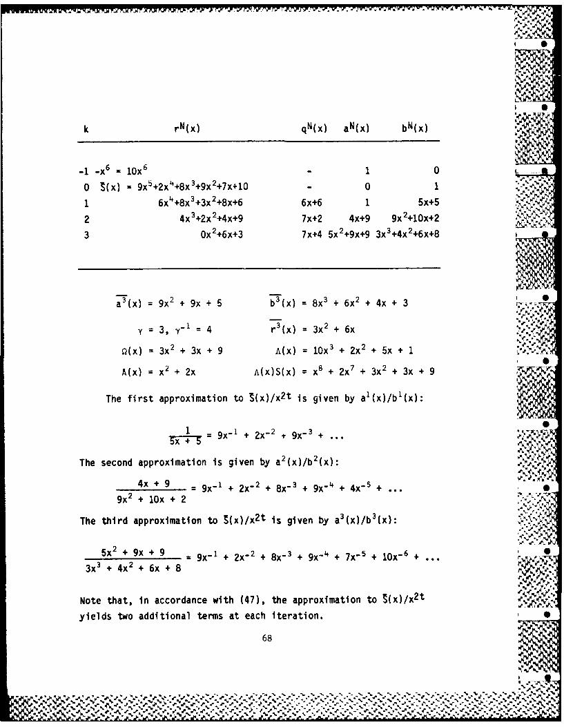
k rN(X) qN(x) aN(x) bN(X)

-1 -X 6 = OX6 -1 0

0 S(x) =9x +2x4+8x +9x +7x+10 04 3-w-

1 6x +8x +3x +8x+6 6x+6 1 5x+5

2 Ux3+2x 2+4x+9 7x+2 4x+9 9X2 +10x+2

3 Ox 2+6x+3 7x+4 5x2 +9x+9 3x 3+4x 2+6x+8

a() x + 9x + 5 b() 8x + 6x + 4x + 3

y= 3, Y- r3(x) =3X 2 + 6x

Q(x) = 3x 2 + 3x + 9 AWx 1 Ox3 + 2x 2 + 5x + 12 8 70

AWx = x2 + 2x A(X)S(x) =X8 + 2x7 + 3x2 + 3x + 9

The first approximation to S(x)Ix2t is given by al(x)/b'(x):

1 =9x- + 2x- 9x- +35x +

The second approximation is given by a (x/b2()

4x + ~ = 9x- + 2x- + 8x- x + 4x- +*.

9 2 10lx + 2

The third approximation to S(x)/x 2t is given by a 3(x/b 3(X):

5x +9x+9 =9x- + 2x- + 8x- + 9x- + 7x- + lox- +

x 0+4U + 6x + 8

Note that, in accordance with (47), the approximation to S(x)/x2t

yields two additional terms at each iteration.

68

% %

Program 5 is less efficient than program 4 because a(x) must 4...

now be retained. For correcting t errors, program 5 typically

requires 3t2 + t multiplications for r(x), t2 + t for b(x), and

- t for a(x) for a total of the order of 5t2. By dropping

unneeded terms of r(x) this total can be reduced to 4t2 . This is

discussed further in section 7.3.

Timing for program 5 is the same as for program 4, assuming 0

that a(x) can be updated sinultaneously with b(x). Under the

assumption of t errors and aeg(q(x)) = i, both programs require 2t

basic time units for their execution, where a basic time unit

represents the time required for one finite field scalar division,

one scalar multiplication, and one scalar subtraction.*( " ,

In conclusion, Mills' algorithm and the Japanese decoding algo-

rithm are seen to be versions of Euclid's algorithm which differ

only in their initial conditions and termination rules. The

Japanese algorithm gives identical results to Mills' algorithm if

the order of the syndromes is reversed, and vice versa. We are

really dealing with one algorithm. S

69

v' .. ,.-:

-" %- % ,.% 6, %

SECTION 6

THE BERLEKAMP-MASSEY ALGORITHM

In this section the Berlekamp-Massey decoding algorithm is

reviewed. The algorithm was originally formulated by Berlekamp [10)

for solving the key equation (14). Massey [11] rederived the

algorithm as a method for synthesizing the shortest-length linear

feedback shift register which will generate a given sequence. We

shall follow Massey's development. a.

Figure 1 is an illustration of a linear feedback shift-register

(LFSR) consisting of L stages. Each input sj to the first stage

is a linear combination, '

Ls. = - Y c i s.~ .i 1

spec'fied by the feedback polynomial coefficients ci (i = 1 ,"

L), of the preceding L inputs sj-i (i = 1, ..., L). For our

purpojes, ci and si are elements of the finite field GF(q) for

some q, a prime power. The output from the shift register is taken

from the last (Lth) stage. Thus, the first L outputs so ... ,

SL-1 are identical to the initial contents of the shift register.

An LFSR is said to generate a finite sequence so, SN- 4N

when this sequence coincides with the first N outputs for some

initial loading of the LFSR. If L > N, the LFSR always generates

the sequence, independent of the coefficients ci. If L < N, the

LFSR generates the sequence if and only if

Ls. + cis i = 0 (j = L, L+1, ... , N-i). (51) •

71 %a

% N-~% *'•~ ~~ % , . %-.. , -44N , - . . > ? %, .r,'. , ,- - ,-w ,'',"' w ,' ' w '?' '.,,- '.-" , ,'

%l

.%.

we SI-.

U7,

% %% % %

Equation (51) is the same as equation (11) relating the

syndromes Sj to the error locator polynomial coefficients Ai.

Thus, for known A, equation (11) is the equation of an LFSR which

generates the syndromes. We want to find a A(x) with lowest degree

v (i.e., fewest errors consistent with the decoding equations).

Therefore, we seek the shortest LFSR that generates the sequence of

syndromes.

We begin with the statement of Massey's Theorem 1 (for a proof,

see [11]).

THEOREM: If an LFSR of length L generates the sequence so, ... , ,*.

SN-1, but not the sequence so , ., SN, then any LFSR that

generates the latter sequence must have length L' satisfying

L' > N + 1- L.

Let s denote an infinite sequence so, s1, ..., and let LN(s)

denote the minimum of the lengths of all LFSR's that generate the -

first N symbols so, s, S--, sN-1 of s. Then we have the .

following

COROLLARY: If some LFSR of length LN(s) generates so, ... , , --.

SN- 1 , but not so, .. SN, then

LN+Ils) > maxlLN(s), N + 1 - LN(s)). (52)

Massey's strategy is to develop an LFSR synthesis algorithm that %

satisfies the constraint (52) of the corollary by strict equality.

,.% .. '., I

73 '

Mr.rM

: , 4%fk

S

For a given sequence s, let

(N) (xLN(S)c (x) = + l CN) x i

denote the connection polynomial of a minimum-length LN(S) LFSR

that generates so, -... SN-1 . As an inductive hypothesis, assume

that LN(s) and c(N)(x) have been found for N = 1, 2, ..., n with

equality obtaining in (52) for N = 1, 2, ..., n - 1. We seek

Ln+l(S) and c(n+l)(x) with equality holding in (52) for the caseN = n. From (51) we have 5

.- - wW

Ln(s) (n)0 j = Ln(s), .. , n-1sj + C, cnsj- i =

1 dn j=n

where dn is the discrepancy between sn and the (n+l) s t symbolgenerated by the LFSR of length Ln(s) which generates so,

Sn-1. If dn = 0, then this LFSR also generates so, ... , Sn,and Ln+l(S) = Ln(s) with c(n+l)(x) = c(n)(x). If dn * 0,a new LFSR must be found to generate so, ... , sn. We want to <-.'

construct this new LFSR, with connection polynomial c(n+l)(x), to

satisfy

L (s) = max[L (s), n + 1 - Ln(S)],n+1 n n

%S.

, ... .. % ' ]

and

Ln+llS) nl

sj + l+, c (n+1) = 0 j = Ln+ls), ... , n.

Massey cleverly constructs the desired LFSR by combining the latest

LFSR with the LFSR which existed at the time of the last length e'-

change, using the discrepancy, say dm, produced by that LFSR to

cancel out the discrepancy d,1 produced by the current LFSR.

Let m = the length of the sequence before the last LFSR length

change:

Lm(s) < Ln(s)

L m(S ) 0 J= Lm(S), ...,m- is j + c , s j i d , m

i=1 dm*0 3G1 (53)

and, by hypothesis,

Lm+l(s) Ln(s) =m + 1 Lmls)"

We now rewrite (53) as . ,

n m s 0 j = i 1- Ln(s) + n, ... , n - 1Si-n+m + l c m j n+m-i = ?"'-'

=1dm 0 J = n (54)

(since Lm(s) - m + n = 1 Ln(s) + n).

"U., "U. "

75

% % %U %

%* 10 -

* AA

Define the new connection polynomial c(n+l)(x) by

.'4c n+1 W) = c(n)(x) - dndml1x n-m c W)(W. (55)

Combining (53), (54) and (55) yields

Ln+l(s) (nlSj + CSn+l) j i

Ln(S) Lm(S)sj + c - - dn Sj-n+m + c1 Sj-n+m-i]i=1 i=1

0 for j = L nLn+l, ... , n-1 0 for j = 1-Ln n,...,n-1

d for j = n d 0 for = n •

0 for j =Ln+1 (s), Ln+1+l, ... , n-1

-ddId = for j =n (56)n A

The LFSR of length Ln+l(S) = max(Ln(s), n+l-Ln(s)) generates

the n+1 sequence symbols so, .. , sn and satisfies the constraint

(52) with strict equality.

Figure 2, adapted from Blahut [17] figure 7.3, illustrates the

new shift register construction. n - m new dummy stages are added

to the front end of the old shift register, whose connection

polynomial is c(m)(x), in order to line up its discrepancy dm to

coincide with (and cancel) the discrepancy dn produced at j = n by ..

the current shift register, with connection polynomial c(n)(x).

76

..................................................................................... .~': '. *%* ~ * .* .. ~ * - -- *. . . .

LL0

OFA

I w S%

EE

. 1

%4 .*

'AAN

- N

~%%

When combined, the new resulting shift register will have lengthdetermined by the maximum of the length Lm(s) of the old shiftregister augmented by the number n - m of new stages, and the length

Ln(s) of the current shift register. As can be seen directly fromfigure 2, the jth input sj to the com~bined shift register isgiven by

Ln(s) (n) 1Lm(s) (m= - c1 sj-i - dnd-i'(-sj.n+m - cmsjn+m-i).

Equation (56) provides a constructive proof of Massey's Theorem 2:

THEOREM: If LN(s) denotes the length of the shortest LFSR which

generates so ***, SN1 then

(a) if some LFSR of length LN(S) which generates so, ..

5N-1 also generates so, *.. sN' thenLN+1(s) = LN(S);

(b) if some LFSR of length LN(S) which generates so .,

sN-1 fails to generate so ... , SN, thenLN+1(s) = max(LN(s), N + 1 -LN(s)).

We observe that in case (b):

if Ln (s (n+l)/2, then Ln~ (s) =n + 1 -Ln (s);

if Ln (s > (n+1)/2, then Ln~ (s) Ln (s)

78 "

00 % 0

Program 6 is a representation of Massey's version of the

Berlekamp-Massey algorithm. Inputs to the program are the syndrome

polynomial S(x) and the BCH code error-correction capability t. The

latter is used at line 4 of the recursion in the test for

termination; the former in line 5 for calculating the discrepancy

between the jth syndrome and the jth symbol output by the

current shift register with connection polynomial bN(x).

The connection polynomial c(m)(x) which defines the

shift-register before the last length change is represented in

normalized form by bO(x). This polynomial is defined at line 9 of

the recursion by premultiplying the current bN(x) by the inverse

of the nonzero discrepancy d. (In later sections we shall consider -

versions of the algorithm with this normalization left out.) The

polynomial bO(x) is then updated in each iteration at line 1 of

the recursion by shifting once, corresponding to the creation of a ;

new dummy first stage, and is then ready for use in defining the new

shift register connection polynomial in line 7 of the recursion.

The program path flow is slightly more complicated than for the

Euclidean programs 4 and 5 as a result of the length test and

branching at line 8 and the discrepancy test and branching at 6.

However, both tests are, in a sense, implicit in the Euclidean

programs, as will be seen in section 7.3.

At termination, the error locator polynomial A(x) is given by

bN(x). The error evaluator polynomial P(x) is not immediately

available in Massey's version, and must be calculated by the key .

equation (14). However, as we shall see in the next section, by a

slight modification of program 6 we can also obtain Q.(x) as in the

Euclidean programs.

79

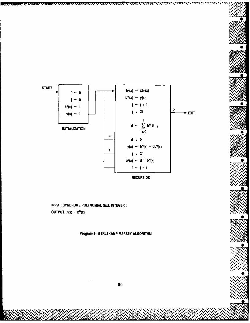
START

bO(x) - xbO(x)

b"(x) - y(x)b O (x ) 1- j / ' +' 0

y(x) 1 j 2t > EXIT

INITIALIZATION d -

d=Od 0y(x) - bN(x) - db°(x)

<A

be(x) - d-I bN(x)

I' "--'-.' -

RECURSION

INPUT: SYNDROME POLYNOMIAL S(x), INTEGER t

OUTPUT: A(X) = bN(x)

Program 6. BERLEKAMP-MASSEY ALGORITHM

80 %

- r

IN 0

This is an efficient algorithm in terms of the number of

multiplications required. Assuming that Z increases by 1 at every

odd numbered iteration, we require 1 multiplication to compute d at

the first iteration, 2 multiplications at the second and third, 3 at

the fourth and fifth, etc., t - 1 at the 2t - 2nd and 2t - Ist,

and t at the 2tth iteration, for a total of t2 multiplications for

computing the discrepancies. Assuming d > 0 at all iterations, we

need t2 + t multiplications to update bN(x) at line 7 of the

recursion and (t2 + t)/2 to update bO(x) at line 9, for a total of

the order of 2.5t 2 . This can be reduced to 2t2 by avoiding the

normalization by d-1 in line 7, as will be discussed in section

7.2.

Program 6 has the drawback, however, that the updating of b(x)

is held up until the calculation of d has been completed. This

drawback is removed in the programs considered in section 7, but at

the expense of requiring further multiplications. Unlike programs 4

and 5, program 6 cannot be executed in 2t basic time units, and is

not a candidate for implementation in a two-dimensional systolic

array. At each iteration, a varying additional computation time is

required to obtain the discrepancy d.

For illustration of program 6, we use the same example of a

Reed-Solomon 3-error-correcting code over GF(11) as used previously

for programs 4 and 5.

Example 10: t = 3; Let c(x) = 0, v(x) = e(x) = 6x9 + 5x8 + 3x"

S(x) = lOx5 + 7x4 + 9x3 + 8x2 + 2x + 9.

81

',~~~ %I.~-

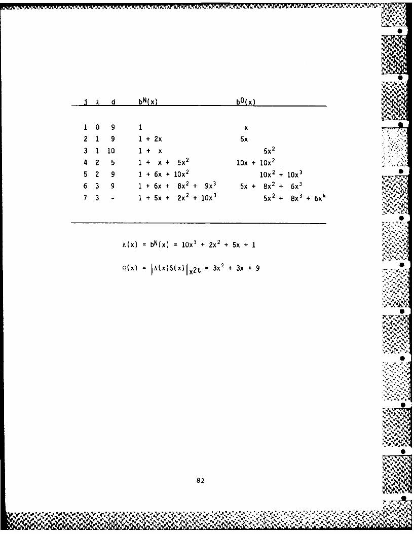
i d bN(x) bO(x)

1 0 9 1 x

2 1 9 1 + 2x 5x

3 1 10 1 + x 5x2

4 2 5 1 + x + 5x2 lOx + lOx 2

5 2 9 1 + 6x + lOx 2 lox 2 + lOx 3

6 3 9 1+6x + 8x2 + 9x 3 5x + 8x2 + 6x 3

7 3 - 1 +5X+ 2x2 + lOx3 5x2 + 8X3 + 6x;N %

A(x) = bN(x) = lOx3 + 2x2 + 5x + 1

Q(x) = x)s(x)Ix2t = 3x5 + 3x + 9 .

WeN

82'

01S

1&0* al,

... ,.

SECTION 7

HYBRIDS AND COMPARISONS

In this section, which contains the main results of this

report, comparisons are made between the Berlekamp-Massey algorithm

and Euclid's algorithm (in the Mills version). Hybrid programs are

developed which combine features of both algorithms to advantage. 0

The section is divided into five parts. First, the Berlekamp-Massey W.,

algorithm is expanded in a Euclidean context. Second, a new

algorithm developed by Todd Citron [22] is examined and shown to .

belong to this same class. Third, Luclid's algorithm is modified to -

replace polynomial division by a sequence of partial divisions.

Fourth, Mills' algorithm is modified to make it more closely

resemble the Berlekamp-Massey algorithm. Fifth, comparisons are

made among the resulting hybrid algorithms, which are then seen to

be very similar. This similarity has been noted previously by Welch

and Scholtz [14], as well as others.

7.1 THE BERLEKAMP-MASSEY ALGORITHM III EUCLIDEAN DRESS

Our objective in this section is to expand the Berlekamp-Massey

algorithm in a Euclidean context. Welch and Scholtz [14] have noted

a correspondence between partial results obtained for bN(x) at

certain iterations of the Berlekamp-Massey algorithm (program 6) and

partial results obtained for bN(x) at successive iterations of

Mills algorithm (program 5). To explore this relationship further,

we introduce polynomials a(x) and r(x) for the Berlekamp-Massey

algorithm analogous to the polynomials a(x) and r(x) of Mills'

algorithm.

83

Io .I . I

% %1? %%

In program 6, the next value for bN(x) is defined at line 7

of the recursion by

y(x) bN(x) - dbO(x). (57)

Let us replace y(x) in (57) by a polynomial bT(x). In a similar

fashion new values will be defined for aN(x) and rN(x) at each

iteration by

aT(x) + aN(x) - daO(x)(58)

rT(x) + rN(x) - drO(x).

At line 9 of the recursion of program 6 a new bO(x) is defined by

bO(x) + d-lbN(x). (59) -" %% -

In a similar fashion we now define -l

aO(x) d-laN(x) (0

Finally, lines 1 and 2 of the recursion of program 6 will be V

repeated in like manner for updating aO(x), aN(x), rO(x), and

rN ( x): .

a0 + xa0 (x)

rO - xrO(x) ... ,-.

aN + aT(x)

rN + rT(x)

84

;% % %

Let f(x) and g(x) be given polynomials. If initial values for

a0(x), b0(x), r0(x), ANx), bN(x), and rN(x) are chosen

to satisfy

rO(x) =a0(x)f(x) + bO(x)g(x) (61) .

rN(X) = aN(x)f(x) + bN(x)g(x) (62)

S

all iterations. Let ak(x), bk(x), and rk(x) denote the values Uof at4(x), bN(x), ana rN(x) defined at the kth iteration ofthe algoritho. Then for all k

rk(x) =ak(x)f(x) + bk(x)g(x) (63)

for the Berlekarip-Massey algorithm. This is the same relationship

that holds for Euclid's algorithm (25), even though the recursions

differ. For f(x) and g(x) in (63) we shall choose

f(x) =-

and

g(x) =xS(x)

converting (63) to

rk(x) = -ak(x) +bk(x)xS(x), k =1, .. ,2t. (64)

85

.1~~N. J.. 0 %f

% % *''** .. % %% %%~i

%~~~~~ % . * '.'~ * ~

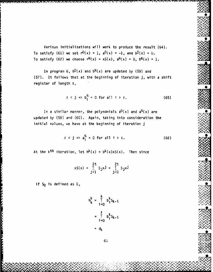
Various initializations will work to produce the result (64).

To satisfy (61) we set rO(x) = 1, aO(x) = -1, ana bO(x) = U.

To satisfy (62) we choose rN(x) = xS(x), aN(x) = 0, bN(x) = 1.

In program 6, bO(x) and bN(x) are updated by (59) and

(57). It follows that at the beginning of iteration j, with a shift

register of length X,0

R < j => bN = 0 for all i > R. (65)1

Ix

In a similar manner, the polynomials aO(x) and aN(x) are •

updated by (58) and (60). Again, taking into consideration the

initial values, we have at the beginning of iteration j

< => aN = 0 for all i > X. (66)1

At the kth iteration, let hk(x) = bk(x)xS(x). Then since

2t 2t

xS(x) SjxJ SjxJj=1 j=0

if So is defined as 0, 0

k =k kh = b Sk-i

= dk i~k-i

83Oe~

V V%%%..%~.~ - .d d.

~~q'_- -A''V

S

and by (64)

r _a k + h = 0 + h = dk. (67)

Therefore, if we keep r(x), we eliminate the inner-product

computation of the discrepancy d.0

Program 7 is a representation of the Berlekamp-Massey algorithm

in a Euclideanized version. We, perhaps wastefully, introduce three

temporary polynomials, denoted by aT(x), bT(x), and rT(x), for

temporarily holding the new versions of a(x), b(x), and r(x) created -

at lines 11-13 of the recursion. Observe that at each iteration j,

r = o. At line 17, r0 is set to 1; if the normalization by d-1

were not performea, its value would be d. After the next

incrementation of j, r9 is still equal to 1; if normalization were .

not performed at line 17 it would still have the value d = dn. At

line 13, rJ is set to 0. At termination, A(x) is given by bN(x)N

and rN = 0 for i = 1, 2, ..., 2t. Equations (14) and (64) jointly

imply that

)(X) : 1(aN (x) + rN (x))/xlx2t

so that 0(x) = aN(x)/x and rN(x)/x = A(x)x 2t. Thus the S

expanded version of the algorithm provides both the polynomials 0(x)

and A(x) in addition to the error locator polynomial k(x) obtained

in Massey's version.

To illustrate program 7 we again use the Reed-Solomon

3-error-correcting code over GF(11) which was used to illustrate

8 7

--------- so, b0(x) - xb0(x)

o 80(x) .- x80(x)

I r0(x) - xr0(x)

r T() -S(X)b"(x) -bT(x)80(x) -1a8(X) - aT(X)

aT~x - 0r"N(x) - r T(X)

b ()-2t >- --- EXIT

INITIALIZATION d-jd 0

bV(x) -b"(x) - dbO(x)

aT(x) -aN(x) - da0(x)

r T(X) -r"(x) - dr0(x)

b0(x) - d -I bN(X)

a0(x) - d-l aN(X)

r0(x) .- d -Ir(x)

RECURSION

INPUT: SYNDROME POLYNOMIAL S(x), INTEGERt

OUTPUT: A(X) b bN(X), fj(X) ON(X)/X.. ..

Program 7. EUCLIDEANIZED BERLEKAMP.MASSEY ALGORITHM

0

88 1-d% % f% 'p% k

% % %

programs 4-6. The polynomials rN(x), rO(x), etc., shown are

those defined prior to the next incrementation of the index J, i.e.

after execution of lines 1-6.

Example 11: t = 3. Let c(x) = 0, v(x) = e(x) = 6x9 + 5x8 + 3x3.

S(x) = lOx 5 + 7x4 + 9x3 + 8x2 + 2X + 9.

j-0, - 0.

rN(x) = xS(x) = lOx 6 + 7x5 + 9X4 + 8x3 + 2x2 + 9xrO(x) = xbN(x) = 1

b0(x) = 0aN(x) = 0

aO(x) = -x = lOx

J=1, 0, d = rN = 9, d- I = 5

rN(x) = lOx 6 + 7x5 + 9x4 + 8x3 + 2x2

rO(x) = 6X7 +2X6 + X 5 + 7x4 + lOx 3 + X2

bN(x) = 1

bO(x) = 5xaN(x) = 9xaO(x) = 0

No

j 2,1=1, d =r2 2 . :

rN(x) = lOx 7 + 6x6 + 5x5 + 6x4 + lOx 3

rO(x) = 6x8 + 2x7 + x6 + 7x5 + lOx4 + x3

bN(x) - x+ 1

bO(x) = 5x2 L

aN(x) = 9x

aO(x) = 0

89

P'.P r % - P W

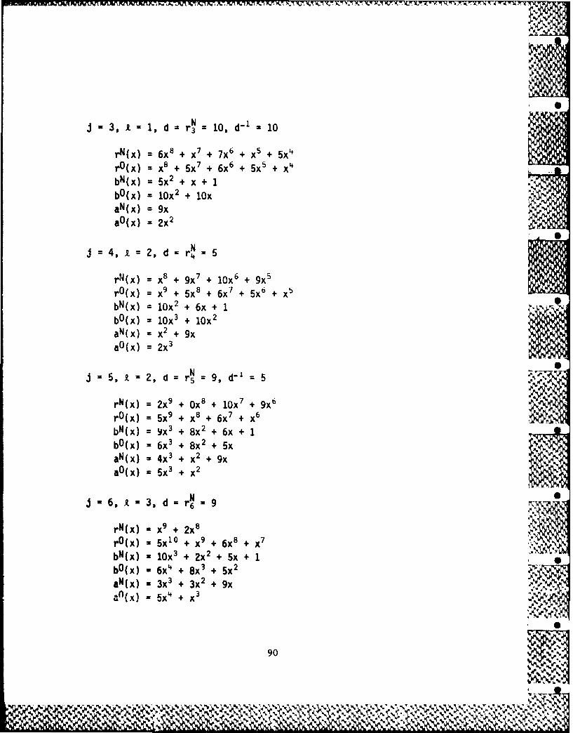
3,= 1, d rN 10 =- 10

rN(x) = 6x8 + x7 + 7x6 + x5 + 5x4

rO(x) = x8 + 5x7 + 6x6 + 5x5 + x4

bN(x) = 5x2 + x + 1

bO(x) = lOx 2 + lOxaN(x) = 9xa0(x) = 2X2

=4, A =2, d = rN = 5

rN(x) = X8 + 9x7 + lOx 6 + 9X5

rO(x) = x9 + 5x8 + 6x7 + 5x6 + x'

bN(x) = lOx 2 + 6x + 1bO(x) = lOx 3 + lOx

2

aN(x) = x2 + 9xaO(x) = 2X

3

5, A = 2, d = rN = 9, d-' = 5

rN(x) = 2x9 + Ox8 + 1Ox 7 + 9X6

rO(x) = 5x9 + x8 + 6x7 + x6

bN(x) = 9X3 + 8x2 + 6x + 1bO(x) = 6x3 + 8X2 + 5x

aN(x) = 4x3 + x2 + 9xaO(x) = 5X3 + X2

N06, 3. d = r6 9

rN(x) = x9 + 2xr0(x) - 5x"0 + x9 + 6x8 + X

bN(x) . lOx 3 + 2x2 + 5x + 1bO(x) - 6X4 + 8x3 + 5x2

aN(x) - 3x3 + 3x2 + 9x()X = 5x4 + x3

90

-p % ~ ' % ~ *

j =7, exit

A(X) = bN(x) = lOx 3 + 2x2 + 5x + 1

o(x) = aN(x)/x = 3x2 + 3x + 9 h

x2tA(x) = rN(x)/x = x8 + 2x7

A(X) = x2 + 2x

The price paid for retaining the polynomials a(x) and r(x) in

addition to b(x) is add4tional multiplications. If all coefficients

of rN(x) and rO(x) are retained, then to update rT(x) at the

first iteration takes one multiplication, and at each subsequent

iteration j takes 2t + 1 - Ij/2j for a total of 3t2. To update

rO(x) requires 2t - Ij/21 multiplications at each odd iteration j

(assuming t is incremented at each odd iteration) for a total of

(3t2 + t)/2 multiplications. However it is not necessary to retain

coefficients above those for x~t. Dropping these, 2t2 - t + 1. ,6

multiplications are required to update rT(x), and t2 + t to update

r0(x). In addition, t2 + t multiplications are required to update

bT(x), t2 - t for aT(x), (t2 + t)/2 for bO(x), and (t2 - t)/2

for aO(x), giving a total on the order of 6t2.

The updates of all polynomials can now be performed in

parallel, however, so that processing time is now 2t basic time

units, as for programs 4 and 5, where a basic time unit represents

the time required for one finite field multiplication and one

subtraction plus (half the time) one finite field inversion. ."-.,"

91

.:;.,.. I,

l444

4 4 *..4?..(Nv--'

9A

7.2 CITRON'S ALGORITHM

Todd Citron has presented a new algorithm [221, based on Kung's

generalized Lanczos recursion [23,24] and related to Schur's

algorithm [25,26), for solving the key equation (14). In this

section we shall not attempt to reproduce Citron's derivation, but

shall simply state Citron's algorithm using his notation and show

that it belongs to the class of Euclideanized Berlekamp-Massey 0

algorithms developed in section 7.1.

Citron describes his algorithm using matrix notation instead of

employing polynomials over finite fields. The elements of his

matrices correspond to the coefficients of our polynomials, as will

be shown. Citron retains three two-columned arrays: R(i),

corresponding to r(x), P(i), corresponding to b(x), and T(i),

corresponding to a(x). Citron's algorithm is stated as follows: S

Recursion: At ith iteration

z-VRz(i- o - z-'R2 (i-1)

= 1 L ~ R~ -1) (68)Iji Yi j1y)Rli1

z-:P2(i -1 0 1 ]Pi z'P2(i-1)Z (69) ". '.PL (i) 0 1 (1-yi) L Pl(i-1) ;..:.....,,.

= 0 r 1(70)TIFz0 1 Yj 1) ji1

92

-O- v y -0 ,

1P ; , o1

'. " " . .. " ", W :-, ",W," " 5 ,;K,.' - . " ..,e-.'v, w ,,.', "",';," ' ",", '. ,," ' 's', ,,,;e_ y % , ,a" ","'V

where z-1 denotes a left-shift operation (one place),

Pi = "top element" of z-lR 2(i - 1)/"top element" of R1(i - 1), (71)

-Ni if Ni > 0 and oi 0

Ni otherwise

1 if Ni > 0 and pi* 0

and yi = (72)

0 otherwise

Initialization:

z-1R2 (0) = [S1 S2 ... S2t]T

R1(O) = [1 0 ... o]T

Z 1P2(0) = EQ 0 . 1]T

pl(O) = [0 ... O]T (74)

zQIT2(O) = 10 O.. 0-1-(75)

Ti(O) [0 0 _1] T ...

At termination:

z'P 2(2t) [o A1 ... A2t3T % %

(76)z' T2(2t) [Qo Q, • t T

93 %. % %N

Let us first apply Citron's algorithm to ou~r Reed-Solomon3-error-correcting code (over GF(11)) example. Then we shall show

that Citron's algorithm is a slight modification of theEuclideanized Berlekamp-Massey algorithm of program 7. For the -

example, we display Citron's columns as rows. By (73) we need 2tplaces for RMi, and starting from (74) and (75) we need 2t + 1

places for PMi and T(i), since 2t left shifts will be made by the

algorithm employing (69) and (70).

Example 12: t = 3; c(x) = 0, v(x) =e(x) =6x 9 + 5x8 + 3x0SWx = lox5 + 7x4 + 9,0 + 8x2 + 2x + 9.

r_1R2(0) = (9, 2, 8, 9, 7, 10)RI(0) = (1, 0, 0, 0, 0, 0)

1 1: Pi 9/1 =9S

N= 1

z-'R2 (1) =(2, 8, 9, 7, 10, 0) 0RIM) (9, 2, 8, 9, 7, 10)

Z_ P2(1) =(0, 0, 0, 0, 0, 1, 0)P1(1) =(0, 0, 0, 0, 0, 0, 1) :

z'1T2(l) =(0, 0, 0, 0, 0, 9, 0)T1(1) =(0, 0, 0, 0, 0, 0, 0)

1 =2: P2=-2 /9 =10

N2 = 0

Y2 0

94%~L

N N N N -V., -J. .

*% ~ **%~* N~. N

z-'R 2(2) = (10, 6, 5, 6, 10, 0) 0Rj(2) = (9, 2, 8, 9, 7, 10)

z-IP2(2) = (0, 0, 0, 0, 1, 1, 0)Pl(2) = (0, 0, 0, 0, 0, 0, 1) .

z' T2(2 ) = (0, 0 , 0, 0, 9, 0, 0 ) . s, ,.d*T1(2) = (0, 0, 0, o, o, o, o)

1 3: P3 = 10/9=6N3 = 193 = -1Y3 -1

,,

z-lR 2(3) = (5, 1, 7, 1, 6, 0)R1(3) = (10, 6, 5, 6, 10, 0)

z-lP 2(3) = (0, 0, 0, 1, 1, 5, 0) ..

P1(3) = (0, O 0, 0, 1, 1, 0)

z-lT 2(3) = (0, 0, 0, 9, 0, 0, 0)T(3) = (0, 0, 0, 0, 9, 0. 0)

1= 4: P4 = 5/10= 6

N4 = 0 V1%

R4u - 0If 4 0 m'

Z'lR 2(4) = (9, 10, 9, 1, 0, 0)RI(4) (10, 6, 5, 6, 10, 0)

z-IP 2(4) - (0, 0, 1, 6, 10, O, 0)P1(4) = (0, 0, 0, 0, 1, 1, o)

z'lT2(4) = (0, 0, 9, 1, 0, 0, 0) I .T1 (4) = (0, 0, 0, 0, 9, 0, 0)

95

.'/'f' op 0-?F. eF.-4.% %<

1 5: P5 =9/10 2

N5 =1

Y5

r lR2(5) = (9, 10, 0, 2, 0, 0) i.

R1(5) = (9, 10, 9, 1, 0, 0)

z-lP(5) (0 1, , 8 9, , 0

'P1(5) = (0, 0,1, 6, 810, 0, 0)

z'lT2 (5) = (0, 9, 1, 4, 0, 0, 0)T1(5) = (0, 0, 9, 1, 0, 0, 0)

16: P6 = 9 /9 =1

N6 = 0

Y6 0

Z- R2(6) =(0, 2, 1, 0, 0, 0)R1(6) =(9, 10, 9, 1, 0, 0) 0

z'lP 2(6) =(1, 5, 2, 10, 0, 0, 0) =(A 0 , A20,P1(6) =(0, 0, 1, 6, 10, 0, 0)

r'lT2(6) =(9, 3, 3, 0, 0, 0, 0) =(00, 9*~ 20)T1(6) =(0, 0, 9, 1, 0, 0, 0)

96 N

MO N 7.NU177-.7 -T77 F.77777 W7-2 VV-71~mJV

P. %

A coparson ithexaple 1 sows hatthecompnens o

Z-'R(i) Z-'2(i, ad z-T2(), ae te sme a th coeficent

of ~ ~ ~ ~ ~ ~ ~ ~ ~ ~~~~. Axb~) n Nx bane tteihieaino

program 7.

A. comparhisaston wth eape show s that theon' componlent ofi

z1-R2(i), where(i, and -tei) aret o the sme -eise as thecins.ofinin ofxb~xad Nx banda the ith iteration ofth elkm-asy lgr h.

progam 7. Cto)=i- Qij(asy

Weof now asserto an laei hl hw hta ahieaini

Cirnsoi faCnyifrn Maseys ih icrpac d

b) Aswhere lemma is te legof th shf-egse atth

Laema: Nnit1n > 0 ad -1 (Mssy =>i 2o- 0- add-

Proo: byindutionon7

or It,A) Vei

Cirn %Mssey:

Citron: Massey: length change required.' "

Rn-i -Nn-i -n + 1 + 2. n_2 qn-i = n - i- In-2 ,',

Nn = Rn-1 + 1 = -n + 2 + 2-zn_ 2 n - 2R.n_ 1 = n - 2(n-1-4-_2 ) '

= -n + 2 + 2Rn_ 2

Case 2: Nn_ 1 <0 or Pn-1 = 0 => 24n_ 2 .1 n-1 or dn_ 1 = 0, ,-,,..

Citron Massey: no length change qire

Nn-1 = Nn-1 1n-1 = Xn-2 1 n

Nn = n_1+1 = Nn l+l N-2-n-1 =n-2ln- 2 = Nn.l+l

Therefore, truth of the lemma for i =n - 1 implies truth for

i =n.

Therefore, by induction on i, the lemma must be true for all i.

This result implies that for all iterations i Citron's

definition of yi is equivalent to - .

1 if = i * 0 an 2R < i

0 otherwise i

where i is Massey's shift-register length (not explicitly computed----z

in Citron's algorithm). yi is a logical variable employed by ..-Citron to eliminate branching. This may be important for VLS

I'

Thpeeoetuth of the alemimo bu to 1om ime t ut he for i

going on. For purposes of comparing algorithms we e falthe .

branching explicit in our programs. i on tn

98

S

The first matrix on the rhs of (68) produces

[z-lR 2(i),R(i)]T on the lhs instead of [R2(i),R1 (i)]T.

Removing this matrix multiplication to get at the recursion proper,

we have

R2(i) = z- R2(i-1) - pi1 (i-1) (78)

and

z-lR 2 (i-1) if oi t 0 and 29 < i

R1(i) = (79)

RI(i-1) otherwise

Citron shifts the arrays R2(i), P2(i), and T2(i) at each

iteration one place to the left, but does not shift R1(i), P1(i),

and Tj(i). On the other hand, in program 7, the polynomial

coefficients for rO(x), bO(x), and aO(x) are shifted once to

the right at each iteration (lines 1-3 of the recursion) while

rN(x), bN(x), and aN(x) are not shifted. Thus, the components

of R2(i), etc., bear the same relation to the components of R1(i),

etc., as the coefficients of rN(x), etc., to the coefficients of

rOW), etc. (Note, however, that at the ith iteration, the

component of R2(i) which corresponds to is now at the "top" of

the array.)

In order to compare Citron's algorithm with program 7 we should

like to remove his left shift of R2(i) and insert in its stead a

right shift of R1 (i). First, let us multiply relations (78) and

(79) by the right shift operator z, yielding

99

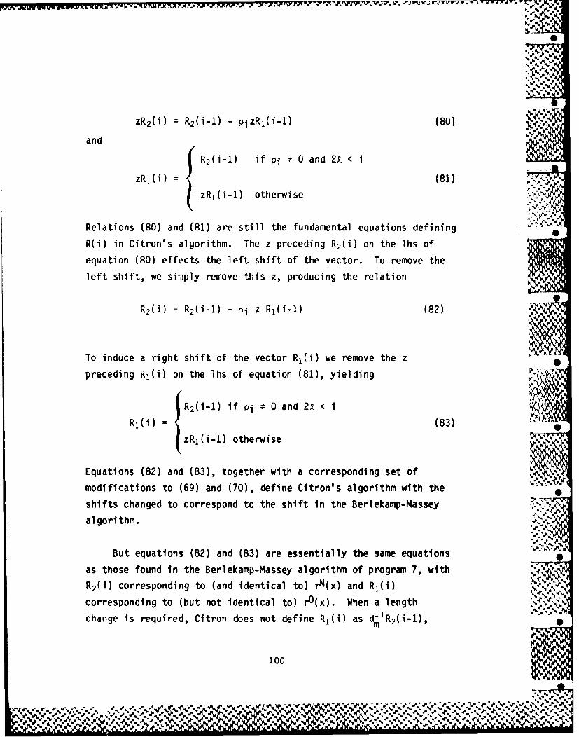
zR2(i) = R2(i-1) - PizR1(i-1) (80)

and

n R2 (i-1) if Pi 0 and 21 < i

zR1(i) = (81)

zR,(i-1) otherwise

Relations (80) and (81) are still the fundamental equations defining

R(i) in Citron's algorithm. The z preceding R2(i) on the lhs of

equation (80) effects the left shift of the vector. To remove the

left shift, we simply remove this z, producing the relation

R2(i) = R2(i-1) - oi z Rl(i-1) (82)

To induce a right shift of the vector R1(i) we remove the z P

preceding Rz(i) on the lhs of equation (81), yielding

R2(i-1) if Pi * 0 and 2R < i

R1(i) = (83)

zR(i-1) otherwise

Equations (82) and (83), together with a corresponding set of

modifications to (69) and (70), define Citron's algorithm with the

shifts changed to correspond to the shift in the Berlekamp-Massey

algorithm. ';'

But equations (82) and (83) are essentially the same equations

as those found in the Berlekamp-Massey algorithm of program 7, with i

R2(1) corresponding to (and identical to) rN(x) and Rj(i)

corresponding to (but not identical to) rO(x). When a length

change is required, Citron does not define RIM as d;'R 2(i-1),

100

r or , W, r " " , " • = " , W " " """". - - - ,4 -",". " "' "" w w" ' 4 " - i

%, .,, % %

as on line 17 of program 7, but simply as R2(i-1). Therefore, when

R2 is updated, it must be updated not as R2(i-1) - dnzR 1(i-1), but

as R2(i-1) - dnd-'zR(i-1). Thus, pi in Citron's algorithm is

the ratio of the current dn, given by the top element of R2(i-1),

diviaed by the old dm , given by the top element of R1 (i-1), and

pi * 0 if and only if dn * 0, as asserted.

Program 8 is a representation of the shifted version of

Citron's algorithm employing (82) and (83) with branching (at lines

10 and 14 of the recursion) shown explicitly. We now repeat our

Reed-Solomon GF(11) example for program 8. A comparison of the

polynomials rN(x), rO(x), bN(x), bO(x), a1 (x), and aO(x)

with Citron's arrays z-1R 2 (i), R1(i), z-P 2(i), Pl(i), z-T 2 (i), and

T(i) shows them to be identical (except for shifts and directions). ., "

Example 13: t = 3; c(x) = 0, v(x) = e(x) = 6x9 + 5x8 + 3x3

S(x) = lox5 + 7x4 + 9x3 + 8x2 + 2x + 9.

i = 0, 9 = 0

rN(x) = lOx 6 + 7 xb + 9x4 + 8x 3 + 2x 2 + 9x

rO(x) = xbN(x) = 1

b0 (x) = 0aN(x) = 0aO(x) lOx

N 0i = 1, 1 = 0: d = rl/r 1 = 9/1 = 9

rN(x) = 1Ox 6 + 7X5 + 9x4 + 8x3 + 2x2

tO(x) = lOx 7 + 7x6 + 9x5 + 8x4 + 2x 3 + 9X2

bN(x) 9x

aN(x) = 9xaO(x) =0 10

, i101

START

---------- 0----- op b0(x) - xb0(x)

0 sp(x) - xS0(X)

rO~x) -r 0(x) - xr0(x)

80(x)- -bN(X) - bT(X)

a T(X - 0rlN(x) - rT(X)

b ()-j 2t EXITd - f~/r?

INITIALIZATION-d 0

bT(X) - b"(x) - db0(x)

a T(X) - UN(x) - da0(x)

rT(x) *- r'4(x) - dr0(x)

b0(x) - bN(x)

a0(x W- a"(x

r0(x) - r'4(x)

RECURSION

INPUT: SYNDROME POLYNOMIAL S(x), INTEGERt

OUTPUT: A(X) =bN(X), (X) = SN(X)IX

Program 8. CITRON'S ALGORITHM

102

'~w 9

I=2, 1=1: d r2/r 2/9 =10

rN(x) = lOx 7 + 6x 6 + 5x 5 + 6X4 + lOX 3

r0(x) = lOx8 + 7x 7 + 9x 6 + 8x 5 + 2x 4 + 9x 3

bN(x) = x + 1b0(x) = x 2

aN(x) = 9x

a0(x) = 00

I=3, 1 = 1: d =r N/r3 :10/9 =6

rN(x) = 6x 8 + X7 + 7x 6+ x5 + 5x 4

r0(x) = lOx8 + 6X7 + 5X6 + 6x5' + lOX 4

bN(x) = 5x2 + x + 1~.b0(x) = x2 + X

aN(x) = 9xax)= 9X2

aO~NO

j 4, =2: d =rN /ro 5/10 =6

rN(x) = x8 + 9x 7 + lox 6 + 9x 5

rO(x) = lOx 9 + 6x 8 + 5x 7+ 6x 6 + lox 5

bN(x) = lOx2 + 6x + 1b0(x) = x3 + x2

aN(x) = x2 + 9xa0(x) = 9x 3

0

103

*PI 4vN LP w w' r

s, M1KI.~

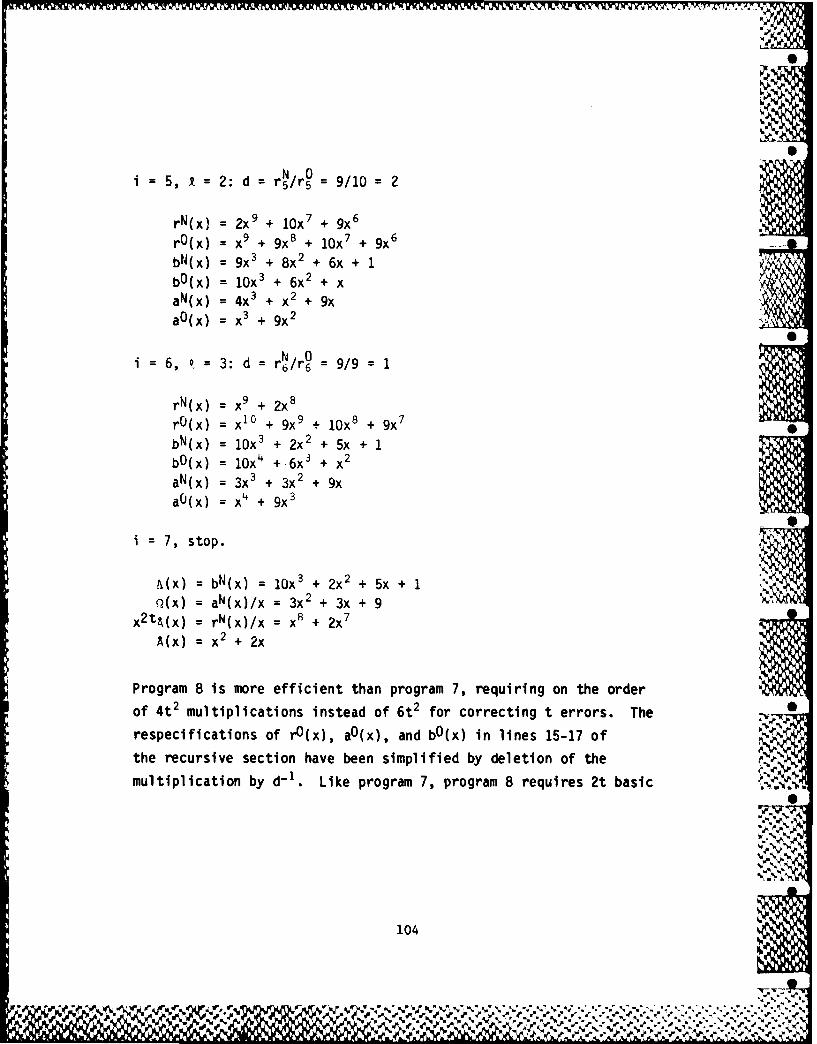
NO0i = 5, 1 = 2: d = r5/r5 = 9/10 = 2

rN(x) = 2x9 + lOx 7 + 9x6

rO(x) = X9 + 9X8 + lOx 7 + 9x6

bN(x) = 9x3 + 8x2 + 6x + 1

bO(x) = 1Ox 3 + 6X2 + xaN(x) = 4x3 + x2 + 9xaO(x) = x3 + 9x2

N 0i = 6, 9 = 3: d = r6/r6 = 9/9 = 1

rN(x) = x + 2x8

rO(x) = xI0 + 9x9 + lOx, + 9x,DN(x) = lOx 3 + 2x2 + 5X + 1bO(x) = 10X4 +.6x' + X2

aN(x) = 3X3 + 3X2 + 9X

aO(x) = x4 + 9x3

i = 7, stop.

.k(x) = bN(x) = lOx 3 + 2x2 + 5x + IQ(x) = aN(x)/x = 3X2 + 3x + 9

x2t&(x) = rN(x)/x = x8 + 2x7

A(x) = x2 + 2x

Program 8 is more efficient than program 7, requiring on the order

of 4t2 multiplications instead of 6t2 for correcting t errors. The •

respecifications of rO(x), aO(x), and bO(x) in lines 15-17 of

the recursive section have been simplified by deletion of the .2multiplication by d-1 . Like program 7, program 8 requires 2t basic PI..N

0

104

r -. r -'p.~~ v r %F .'". %v %*~~~~~ % .I rP. -e %.r ~% \fI g

time units, but a basic time unit now includes a finite field

division at every iteration (instead of a finite field inversion at

alternate iterations) as well as a multiplication and a

subtraction. Any way you look at it, however, this is still the

Berlekamp-Massey algorithm. Citron's achievement has been, not to

derive a new decoding algorithm, but to show an equivalence between

the Berlekamp-lassey algorithm and Kung's generalization of Lanczos'

algorithm.

7.3 INSIDE EUCLID'S ALGORITHMl

In this section we revisit Euclid's algorithm for polynomials 9

(program 3) in order to take apart the polynomial division defined

in the first step of the recursion

q(xl - LrO(xl/rN(x) (84) 9

To keep things as simple as possible, we shall work with the

original version of Euclid's algorithm rather than with the extended

version which obtains a(x) and b(x). We wish to replace the

polynomial division of (84) by a sequence of k + 1 partial divisions

where k is an integer defined by

k = deg(rO(x)) - deg(rN(x)) = deg(q(x)) (85)

Except at the initial iteration, where rO(x) = f(x) and rN(x) = ,g(x) may result in k = 0, we have k > 0 for all polynomial divisions

(84). Usually after the first iteration of program 3, though not

always, q(x) is linear so that k = 1.

105

In performing the sequence of k + 1 partial divisions we do not

want to redefine the divisor rN(x) until the polynomial division,

i.e., the k + 1st partial division, is completed. Until that time,

the new remainder, say rT(x), becomes the next numerator rO(x)

and the divisor rWlx) is unaltered (except for shifting right to

line up appropriately with rO(x)). On the other hand, when the

polynomial division is complete, the new remainder becomes the next

divisor, while the old divisor becomes the next numerator. Thus, we

have

rN(x) xlrN WxA

if not completing k times (86)

r0(x) + r(x) _ qrN(x) a polynomial division

and S

r Wx + r (x) -qr Wx

if completing k + 1st (87)rO) + x-irN W a polynomial division

where q is a scalar defined as the ratio of the leading coefficient

of r0(x) to the leading coefficient of rA(x).

In order to perform the subtractions in (86) and (87) it is

necessary to align the leading coefficients of the polynomials

rN(x) and rO(x). For convenience, we turn the polynomials

arouno and align the trailing coefficients. In this way we can dealwith the coefficients r and r at the jth iteration and define

q as r /r if r 0 0. Specifically, we shall initialize .,K "

106

;Ir N N~~

NV~~

rO(x) by the reversal P(x) of f(x). To properly align rO(x) and

rN(x) as f(x) and g(x) are initially aligned, we initialize

rN(x) by xdg(x), where d = deg(f(x)) - deg(g(x)) is assumed to

be strictly positive.

Program 9 is a representation of Euclid's algorithm for

polynomials (in the unextended version) when each polynomial

division is replaced by a sequence of k + 1 partial divisions, where

k is defined by (85). The polynomials rO(x) and rN(x) have been

initialized by T(x) and xdg(x), respectively. Correspondingly, at

termination, the gcd(1(x), §(x)) is given by r0(x), so that

gcd(f(x), g(x)) is given by r0 (x), as shown in section 3.

Program 9 is not essentially different from program 3, but

shows explicitly what is implied by (84). The recursion is divided •

into two loops, the left one for completing a polynomial division,

and the right loop for continuation of the division. Choice of

which loop to follow is determined by the integer variable i.

Assume that as we complete one polynomial division and initiate

its successor we have j = 2R.. (Observe that j can never be less

than 29., for 9 is incrememented only when j > 2R., and j is

incremented at the same time; on the other hand, if j > 2Y, we stay i _

in the continuation loop.) If deg(rO(x)) = deg(rN(x)) + k

in program 3, then we want to execute the right-hand loop of

program 9 k times, followed by one execution of the completion . , ..-

loop. Before the initial incrementation of j we have rQ = 0, -

r +i 0, and rj+ i = 0 for i = 0, ..., k-i and rj+k * 0.After the initial incrementation of j, r3 * 0. The upper part of

107

' .I , V.n P I V PJi' M'-R? Pr . x,1A ." L 7Xj k -c v ?F)

START

oTR No 0 r(x m x rox) rowx ~- r'(x)

j -0 ,H(X) 4~rT(X) r"(X) ~- er m~

- * CONTINUATION LOOPr0(x)4-f~x) rN 0-2- +

INITIALIZATION q ~-rIrN

rT(x) 4-r0(x) -qrN(x)

:2f

COMPLETION LOOP '

INPUT: POLYNOMIALS Ax), g(x); INTEGER d udog (1(x) - dog (9(x)) >.0

OUTPUT: gad (f(x),g(x)) 77'y(x)

Progrm 9. EUCLID'S ALGORITHM WITHOUT POLYNOMIAL DIVISION

108

%4 ~ ~I"

I

the completion loop is first executed k times; each iteration0increments j and shifts rO(x) once, so that rj is unchanged as j

increases. After k executions, rj , 0, so that we enter the

continuation loop with j = 2t. + k. In the continuation loop,

rN(x) is shifted once at each iteration, so that now remains

fixed and nonzero. We remain in the continuation loop for k

executions, incrementing both j and 1, after which we return to the

completion loop with j = 2. The final remainder rT(x) becomes

the divisor in the next polynomial division, while the current

divisor rN(x) becomes the numerator for the next polynomial

division. Termination occurs when the new divisor rN(x) = 0 after

completion of a polynomial division. For an example illustrating

program 9 we repeat example 2 from section 2.

Example 14: f(x) = x5 + 3x4 + 3x2 + 5x + 10g(x) = 2X2 + 7x + 3 over GF(11)

j = 0,- 2 = 0

rO(x) - x?(x) = lOx 6 + 5x5 + 3x4 + 3x2 + x

rN(x) x (x) = 3x5 + 7x4 + 2x'

j = 1, 1 = 0, rN = 0

rO(x) + xrO(x) = lox7 + 5x 6 +3x5 + 3x 3 + x2 -

j = 2, k =0, N orj

8 7 6 4 3rO(x) xrO(x) = lOx + 5x + 3x + 3x + x

109 IiN-. w > w.fw..D.,..h~ , ) ,L, .w,'- ) ,.'-, ..- ,:--. .:,. ,t

'w." ,-.w DF.- " .%,- -w "hT.W, ,, ,(,.- - ... ,. - -...- -. v

3, 0,rj 2, rQ 1, q= 1/2 =6

rT(x) -r 0(x) - qrN(x) = lOx8 + 5x' + 3x' + 4x' + 5X4

r0(x) + rT(x)rN(x) +- xrN(x) = 3X6 + 7 X5 + 2x'

j=4, 9.=1, Nj = 2, rQ = 5, q = 5/2 =8 .

rT(x) ~- r0(x) -qrN(x) = lox8 + 5X7 +X 6 + 3X5

r0(x) + rT(x)rN(x) - xrN(x) =3X

7 + 7 X6 + 2 X5 .

j =5, =2, rj = 2, rj = 3, q = 3/2 7

rT(x) - rO(x) - qr1l'(x) =lOx8 + 6x + 7x

rN(x) 4-xN(x) = 308 + 7 X7 + X6r~~ - x +

6, 3 r = 2, r? = 7, q = 7/2 =9

rT(x) - r0(x) - qrN(x) =5x8 + 9X7

r0(x) 4- xrN(x) U 3 9 + 7x8 +2X7

rN(x) - rT(x)

=7, =3, =9, =Q2, q 2/9= 10

rT(x) + r0(x) - qrN(x) =3x9 +x

8

r0(x) +rT(x)rN(x) 4- xrN(x) =5x

9 + Wx

1110-% l

N, 0

j 8, 4: r= 9, r= 1, q= 1/9 = 5

rT(x) - rO(x) - qrN(x) = 0

rO(x) + xrN(x) = 5x i o + 9x9

rN(x) + rT(x) = 0

stop

a-gcd(f(x), g(x)) = rO(x) = 9x + 5

e 9, y : 1- = 5 .e

...

gcd(f(x), g(x)) = x + 3

A comparison of this example with example 2 shows that the

sequence of q's defined above is identical to the successive

coefficients of q(x) obtained in the earlier example. .

Program 9 is somewhat awkward because two different loops are S

followed according as we are concluding a completion loop or a

continuation loop. Both loops contain some statements in common,-*

namely, lines 4-8 in the completion box. Both loops define a new

polynomial rT(x) at line 7, and retain this new polyno.iial -

together with one of the pair (r(x), rOlx)). In the

continuation loop rT(x) becomes the new numerator, while the other

retained polynomial (shifted) becomes the divisor; in the completion

loop the assignments are reversed: rT(x) becomes the new divisor,

while the other retained polynomial (shifted) becomes the

numerator. Surprisingly, all that really matters is that the

N -N

11b

w'-*.~~~~~~~ NIP% N %.% *..,...' V.* .. XX d& * * * .,

V I .

correct pair of polynomials be retained. It does not matter which .. w

polynomial is assigned to be the numerator and which the divisor.

We can take advantage of this fact to design an improved algorithm.

Let us first observe that it is permissible to multiply either

rO(x) - rN(x) by an arbitrary scalar B. For if

RO(x) = RrCix)

and

RNx) = vr1M(x)

for some s.ars 9 ana y, then

Rj/RN = (9/y)q

and RT(x) = RO(x) - QRN(x)

= SrO(x) - (P/y)qyrN(x) S

= qrT(x).

Thus the only effect produced by multiplying rO(x) or rN(x) by a S

scalar is to multiply future rO(x) and rN(x) by some scalar.

Next, consider the effect of swapping roles. If the

assignments of polynomials to rO(x) and rN(x) are reversed at 0

some stage, then we shall calculate a new RT(x), say, at line 7 by

112'Y, kl

wr ., ," . w" ,, w ," . , F ,, -- .. ,%-.-" . %, w %, '% . , " % %" '%' % ." " w -, .. , " "' -• @ -" , ,." -' -s

RT(x) = rN(x) - (rN/r5)rO(x)

so that

qRT(x) = -qrN(x) + rO(x) = rT(x)

or

RT(x) = -q-'r T (x).

Thus, reversing the roles of numerator and divisor has no effect on

the algorithm other than a multiplication of the result by a scalar

so long as we take care to retain the correct pair of polynomials at

each iteration.

We are now in a position to eliminate the continuation loop

from program 9, producing an improved version of Euclid's

algorithm. We shall still replace each polynomial aivision by a

sequence of k + 1 partial divisions. After the initial

determination of rT(x) (in a given polynomial division) we otfit

the branch to the continuation loop, define rO(x) by the old

divisor in the last line, and let rT(x) become the divisor at line

2, thus reversing the roles played by rO(x) and rN(x).

Having once defined rO(x) at line 9 of the completion loop,

however, we must not redefine it (except for shifts in line 1) until

the polynomial division is completed. This we can ensure by adding

the statement

113

or, - .% ,*. ¢ . S;,

-. .. ".."*"., S " - . . .....r. . 5. . .. - .. " '. ".. "W~'W / ,~ ,:¢' '7 ,' ' ,' .-. , ,

,¢ , .. ' ,"--"',, " ; ' '"""' , "

."0

to the end of the completion box, and replacing the branch from the

test

j 2.z.

with a branch to the first line whenever the relation is satisfied

by <. The first time through we have j = 2. + k. At the new last

line of the box, 9 is redefined as 9' = j -9 = 9 + k. Thereafter,

the branch test will succeed for the next k iterations, until

j = 2Z + 2k = 2', when the polynomial division is finally 0

completed. During these k iterations the roles of rO(x) and

rN(x) remain reversed. The divisor polynomials of program 9 are "

now numerators, and scalar multiples of the numerators of program 9

are now divisors.

There is one more point to be made. During the k iterationswith reversed roles rQ is fixed and nonzero (as r was fixed and

nonzero 4n program 9). However, it is possible that at some one of •N.

thes- terations r3 is zero, causing a branch to line 1 from

line 5. Th-s is more efficient than the longer path taken in

program 9, where q is defined as 0, rT(x) as rO(x), followed by %

a branch to the continuation loop which redefines rO(x) as 0

rT(x), i.e. as itself. The result is the same; the path taken is

longer in program 9.

Our final version of Euclid's algorithm is given by program 10

and illustrated by example 15, a reworking of examples 2 and 14.

Example 15: f(x) = x 5 + 3X4~ + 3x 2 + 5x + 101-g(x) = 2x2 + 7x + 3 over GF(11)

d=3

114

N N .

STARTo- 0 r'ix) - xr0(x)

j - 0 rN(x) rT(x)

r0(x) .- i(x) rN(x) : 0 EXIT

rT(x) . xdj(x) j -j +1

IN IT IA L IZ A T IO N r . 1 0

rT(x) _ ro(x) - qrN(x)

r(x)- rN(x)

C .- i-C

RECURSION 0

INPUT: POLYNOMIALS t(x), g(x); INTEGER d = dog (f(x)) - dog (g(x)) > 0

OUTPUT: gcd (f(x), g(x)) = yr(x)0

Program 10. SIMPLIFIED EUCLID'S ALGORITHM . .,,

115

r . d .' ~ '• .., - . -'

V P.. . . . .. . ...% V

rN= 0, 9 + x3() +70 x

r 0 (x)~~~ %- xx x x

i' l = O rN =xO

rO(x) 4- xrO(x) = 1x x 3x5 +x 3 + x23

j = 1, t. = 0: 0N= ,rO(x) - xr(x) = lOx + 5x + 3x + 3x' + x

j = 2, , = r N = 0,

rO(x) +xr0(x) = lOx 8 + 5X7 + 3X6 + 3X4 + X

j 3, 0O: rj 2, rj = 1, q = 1/2 =6

rT(x) + rO(x) - qriN(x) = 10x 8 + 5x7 + 3x6 + 4x5 + 5x4

rO(x) + xrN(x) = 3x6 + 7x5 + 2x4

rN(x) *- rT(x)

4, = 3: 5, r 2 q 2/5 = 7

rT(x) + rO(x) - qrN(x) = 7x8 + 9x7 + 4X6 + X5 5

rO(x) + xrO(x) = 3x7 + 7x6 + 2x5rN(x) + rT(x)

j =5,9. = 3: N = 1, r? = 2, q = 2/1 = 2

rT(x) 4- rO(x) - qrN(x) = 8x8 + 7x7 + lOx 6

rO(x) + xrO(x) = 3x8 + 7x7 + 2x6

rN(x) 4- rT(x)

6, Q = 3: rj = 10, rj = 2, q = 2/10 = 9 % %

rT(x) - rO(x) - qrN(x) = 8x8 + lOx 7

rO(x) + xrO(x) = 3x9 + 7x8 + 2x7

rN(x) + rT(x)

116

% % % * .. ..0 %

NNj 7, t = 3: = 10, r= 2, q= 2/10= 9

rT(x) - rO(x) - qrN(x) = 3x9 + x8

rO(x) + xrN(x) = 8x9 + lOx 8

rN(x) 4- rT(x)

j 8, P = 4: rj = 1, rj = 10, q= 10/1 = 10

rT(x) * rO(x) - qrN(x) = 0

rO(x) - xrO(x) = 8x ° + lOx 9

rN(x) + rT(x) = 0

stop

* gcd(f(x), g(x)) = rO(x) = lOx + 8 S0 10, Y 0 1 =10o

gcd(f(x),g(x)) = x + 3

Program 9 is an exact translation of Euclid's algorithm for I%

polynomials when polynomial division is broken down. Program 10 is

cleaner and more efficient than program 9. Program 10 closely '

parallels Berlekamp's decoding algorithm and, in effect, shows why

the Berlekamp-Massey algorithm is more efficient than decoding ,.-

algorithms based directly on Euclid's algorithm. In section 7.4 we aadapt the Mills' decoding algorithm of program 5 to reflect the

changes of programs 9 and 10. The resulting decoding algorithms are . .i-

then shown to be equivalent to the Euclideanized Berlekamp-Massey

algorithm of program 8.

1

7.4 MILLS' ALGORITHM IN BERLEKAMP-MASSEY DRESS

In this section the Mills' decoding algorithm of program 5 is

modified in two stages. First, the polynomial division is replaced

by a sequence of partial divisions as in program 9. The resulting

algorithm is essentially the same as program 5, but is free of

polynomial divisions and can test for termination by counting

iterations. However, like program 9 it suffers from a more

complicated control structure in that the recursive section consists

of two distinct loops. In the second stage we eliminate the

continuation loop, producing an algorithm analogous to program 10.

This version of Mills' algorithm closely parallels program 8 and

might be viewed as its Euclidean reflection. Finally, we show that

these new decoding algorithms are equivalent to the Berlekamp-Massey

algorithm of program 8.

An initial change which we make in program 5 in order to

conform to the initializations of programs 7 and 8 is to reverse the

signs of the initial values of rO(x) and aO(x). In program 5,

this would have the effect of reversing the sign of q(x) at each S

iteration and of r(x), a(x), and b(x) at each odd-numbered

iteration. Since at termination K(x) is obtained as some scalar ..

multiple of bN(x), and 5(x) as the same multiple of aN(x), this

sign reversal may change the scalar but does not affect the S

determination of A(x) and P(x), nor of the error magnitudes.

As in programs 9 and 10, it is convenient to be able to defineON.

q at the jth iteration as rj/rj instead of as the ratio of the S

leading coefficients. To achieve this, we initialize rN(x) by

xS(x) and rO(x) by 1, as in programs 7 and 8, rather than by S(x)

and -x2t , as in program 5. Initialization of rN(x) by xS(x)S

118 7

,~. ,, %. .

START-0 bc(x) - xb0(x) bo(x) - bT(X)

j a0(x) .- xa0(x) a(x) - aT(x)

r0(x) - 1 r0(x) .- xr0(x) r0(x) - rT x

r1(x - x 5(x) bN(x) -bT(X) bN(X) - xb N(X)

80

(x) - - IN(X) -ST(X) a N(X) _ XaN(X)

a T(X) -0 rN(x) - rT(X) rN(x) - xfrd(x)

b0(x) - 0 j - j+ I

bT(X) - 1j 2t CONTINUATION LOOP 9

INITIALIZATION q EI ~b T(X) -b

0(x) - qb N(X)

aT(X) -a 0(x) - qaN(X)

r T(X) -rO(x) - qrN(x)

b0(x) - b N(X)

a0(X) - aNo()

&0(X) - rN(X)

COMPLETION LOOP '9

INPUT: SYNDROME POLYNOMIAL S(x), INTEGERI

OUTPUT: -A(X) = bNX, )Q(X) = 8N(X)/X ~~

Program 11. MILLS' ALGORITHM WITH PARTIAL DIVISIONS

119%

N- "t k -1

means that at iteration 1, rN will be Sj; initialization of rO(x)0by 1 means that at iteration 1, after a right shift of rO(x), r0

will be 1, and the initial q is defined as 1/Sj, as required, 1 and

S, being the leading coefficients of x2t and S(x).

Program 11 is a representation of Mills' algorithm with these

initialization changes when the polynomial division is broken down

into its partial divisions (i.e., program 11 is the Mills' decoder

analog of program 9). This is not a different algorithm from that

represented in program 5, but explicitly shows what is implied by

the first statement in the recursion of program 5

q(x) - [rO(x)/rN(x)J.

The recursion in program 11 is divided into two loops, the left one

for completing a polynomial division, and the right loop for

continuation of the division as in program 9. Choice of which loop

to follow is determined by the integer variable 1.

Termination of the program can now be decided by counting

iterations j and stopping if j exceeds 2t. For, if in program 5

deg(rN(x)) < t then in program 11 r = 0 and the program makes

no further changes except to increment j. Suppose 2t iterations do

not suffice. Each polynomial division with k = deg(q(x)) requires

2k iterations (k shifts of rO(x) followed by k trips through the

continuation loop). Thus, if n polynomial divisions are required,

and ki denotes the degree of the ith quotient polnomial as defined

by (85) for the remainder polynomials of program 5, then

'U]

120

n2 ~k. 2t +2s

where s > 0 if 2t iterations do not suffice.

B t n 1 n -1k k. deg(rK (x)) - deg(r -(x))

-2t - deg(rnll(x))

Therefore,

deg(r n-I (x)) =2t - (t + s)

=t -s< t

leading to a contradiction. Therefore, 2t iterations suffice and

program 11 need not test for the degree of rN(x).

The treatment of r(x) is slightly different from that of

program 5. We need to keep only 2t terms, and at each iteration jwe set rj = 0, leaving only 2t -jcoefficients to be multiplied

at the next update. We thus require only 2t2 + t multiplications

121

%%

for updating rT(x), instead of the 3t 2 + t implied by prog-am 5.In program 5, the number of multiplications could also be reducedfrom 3t2 + t to 2t2 + t by recognizing that terms in r(x) beyond2t - j need not be retained after iteration j. However, this same

reduction cannot be applied in program 4 without losing (?(x) in the

process. 2t basic time units are required in program 11 to correct

t errors, where a basic time unit consists of the time required for

one finite field division, one multiplication, and one subtraction.

We now repeat our Reed-Solomon 3-error correcting code example

for program 11.

Example 16: Reed-Solomon 3-error-correcting code over GF(11) with

a=2.

t =3; let c(x) = 0, v(x) =e(x) =6x 9 + 5x8 + 3x.S(x = lox5 + 7x+9x + 8x2 + 2x + 9

rN(x) = XS(X) = lOx6 + 7X5 +9X 4 + 8X3 2X2 + 9Xr0(x) = x (after shift)bN(x) = 1b0(x) = 0aN(x) = 0

a0(x) = -x =lox

1, =0: =r 1/r1 1/9 =5; execute continuation loop

rN(x) +xrN(x) = Ox7 + 7 X6 + 95+ 8X4 + 2X3 + 9X2

rO(x) 4- rO(x) -qrN(x) =5x6 +9 5 +lx + 4x3 +x

bN(x) - xbN(x) =x

b0(x) +- bO(x) -qbN(x) =6

aN(x) +- xaN(x) =0

a0(x) +- aO(x) -qaN(x) =lox

122

'IN. I p

j=2, =1: q =r2/r2 = 1/9 = 5; execute completion loop

rN(x) - rO(x) - qrN(x) = 5X7 + 3X6 + 8X5 + 3X4 + 5X 3

rO(x) - xrN(x) = lOx9 + 7 X7 + 9x6 + 8X5 + 2X4 + 9X3 ...

bN(x) - bO(x) - qbN(x) = 6x + 6 ...'.bO(x) + xbN(x) = X2 -,

aN(x ) aO(x) - qaN(x) = lox

aO(x) - xaN(x) = 0 .R

3, 1 = : q = r01r 3 = 9/5 = 4; exceute continuation loop

rN(x) = 5x8 + 3x) x + 3x 6 + 8X6 + 3X + 54

rO(x) = 109 + 9x7 + 8x 6 + 9x 5 + x +x 9bN(x) = 6x + 6xbO(x) = X2 + 9x + 9

aN(x) = olx2a 0((x) = 0x

j=4, = 1: q = r3Ir4 = 1/5 = 9; execute completion loop

r (x) = 9x8 + 4x7 + 2x6 + 4x5 +.5x

rO(x) = 5x9 + 3x8 + 8X7 + 3x6 + 5X5 0bN(x) = 2x2 + lOx + 9

bO(x) = 6x + 6x + 9

aN (x) = 9X2 + 4xaO(x) = 1x 3

j = 5, . = 2: q = r5/r = 15 4 = 9; execute continuation loop

rN(x) = 9x9 + 4x8 + 2x 7 + 4 x-

rO(x) = 5x9 + 3x7 + 6x 6 , ... _

3 2

bN(x) = 2x2 + lox + 9xb0(x) = 6x + x +

aN(x) = 9x1 + 4x 2rx)= +OX 4X +2x+4

aO(x) = lOx 3 + 8x 2 + 6x

%

123

. ..- Wf *. % %I %- .'..",';.',,',' ., -.-.- ,,.'.", ,- ,F ., ,.",, , -.- ', .,_ ,,.,.,"', -,, " ' "'t,. . .v -' ' ' '. .

= 6, E = 3: q r /r6 N 6/4 = 7; execute completion loop

rN(x) = 8x 9 + x

rO(x) = 9x I u + 4x 9 + 2x 8 + 4X7 -

bN(x) = 3 3 + 5x + 7x + 8bOx X + 1O3+9XaN(x) = 2X 3 + 2X 2 + 6x

aO(x) = 9X4 + 4X3

j : 7, stop: y = 8, Y-1 = 7

&(x) = y-irN(x) = lOx 3 + 2X2 + 5x + 1n(x) = y- laN(x)/x = 3x

2 + 3x+9: ' ~x2t: (x) , (x)= - irN(x)/x = x 8 + 2X7

20

The computational flow of program 11 is awkward, like that of

program 9. A more efficient algorithm can be obtained by

incorporating the changes of program 10 into Mills' decoding, ,,:

algorithm. Three alterations are made to program 11:

(1) Eliminate the right-hand loop, returning the arrow to the '

top of the left-hand loop.

(2) Reverse the condition for taking the branch from " to•

(3) Add the specification statement,.-;Z;

to the bottom of the left-hand loop. o"

~124

. . . . - - -" "- -%

jN. 004 7, stp % ,y = y'lr~x) =l~x3 +2x. +5x +'

-- ' 'W.V'• ' # ; , ,i - ,) , = ,ylaN .- ,w ,.. , ,,'x)/.x = .3x2 -", , - , -+ 3x. + 9.-, . . -, . .- -. , - .

These changes result in program 12, which is seen to be very similar

to program 8. Like programs 8 and 9, program 12 requires 2t2 + t

multiplications for updating rT(x), and a total on the order of

4t 2 multiplications for finding &(x) when t errors have occurred.

Like programs 8 and 9, program 12 requires 2t basic time units where

a basic time unit includes the time to perform one finite field

division, one multiplication, and one subtraction.

We now repeat example 16 for program 12.

Example 17: Reed-Solomon 3-error-correcting code over GF(11) with :.

a =2. 0

t = 3; let c(x) = 0, v(x) = e(x) = 6x9 + 5xa + 3x3.

S(x) = lOx 5 + 7x4 + 9x3 + 8x2 + 2x + 9

j = 0, . 0:

rN(x) = xS(x) = lox6 + 7x5 + 9x4 + 8x3 + 2x2 + 9x b .

rO(x) = xbN(x) = 1

bO(x) = 0 xaN(x) = 0

aO(x) = -x lox

0 Nj = 1, 0 0: q= r /r1 = 1/9 = 5

rN(x) = 5x6 + 9x5 + lOx 4 + 4x3 + X 2

rO(x) = lOx 7 + 7X6 + 9X5 + 8x4 + 2X3 + 9x2 0

bN(x) = 6bO(x) = x %aN(x) = 10

aO(x) = 0

125

, .1 ', . "- ." - .. • -*•- - - , , " , •d - .

IF " .,,,, '%, ,,%, .%.,"

I

STARTf---0 b°(x) - xb°(x) --

0 aO(x) - xao(x)

r°(x) - I rO(x) - xrO(x)

r(x)- x S(x) bN(x) bT(x)0aN(x) - aT(x) "8T .)-

aT(X) - 0 rN(x) rT(x)b°(x) - 0 j j j+1

bT(x)- 1 j 2t > EXIT

INITIALIZATION r :0q - /r

bT(x) - bO(x) - qbN(x)

a T(x) - aO(x) - qaN(x)

rT(x) - rO(x) - qrN(x)

b°(x) bN(x)• .5-5.%-

aO(x) - a N(x). .-.

r&(x) - rN(x) . .. '

LSRECURSION

INPUT: SYNDROME POLYNOMIAL S(x), INTEGER I

OUTPUT: - A(X) = bN(x), " Q (X) = aN(x)IX . ,

Program 12. SIMPLIFIED MILLS' ALGORITHM N5

126

%.

N N %.% %TI

j=2, .= 1: q r 02/r2 N 9/1 =9

rN(x) = lOx 7 + 6X6 + 5x0 + 6X4 + 10xIrO(x ) = lOx8 + 7 X7 + 9X6 + 8W + 2X4 + 9X3

bN(x) = x + 1bO(x) = X2

aN(x) = 9x

aO(x) = o

O N

j = 1, = 1: q = r3/r3 = 9/10 = 2;

rN(x) = lOx 8 + 9x7 + 8x6 + 9x5 + x4

rO(x) = 108 + 6 7 + 5X6 + 6x5 + lOx •9

bN(x) = x2 + 1x + 9

bO(x) = X2 + X

aN(x) = 4x

aO(x) = 9X2

ON

j = 4, = 1: q = r/r 3 = 10/1 10

rN(x) = 9x8 + 4X + 2x6 + 4X 5

rO(x) = lOx + 68 + 5x7 + 6X6 + lOx,

bN(x) = 2x2 + 9Ox + 9 S,

bO(x) = X3 + x2

aN(x) = 9X2 + UxaO(x) = 9x3

0 Nj 5, i =2: q = r5/r 5 =10/4 =8

rN(x) = lOx9 + OxB + 6X 7 + x6

rO(x) = 9x9 + 4x + 2x7 + 4X6 +

bN(x) = x3 + 7x2 + 8X + 5bO(x) = 2x3 + 2Ox2 + 9X

aN(x) = 9x3 + 5x2 + X

aO(x) = 9x3 + 4X2

127 O

=~~~~ 2: q r5 r 1/=

rN x C. e-x9 +. Ox , ".7 +

j=6, 1 3: q r = r 4/1 =4

rN(x) = 2x 9 + Ux8 PA

r0(x = 9x10 + 490 + 2x8 + 4X7

bN(x) = 9X3 + 4X2 + 10x + 2b0(x = 2X4 + lOx3 + 9X2

aN(x) = 6X3 + 6X2 + 7xa0(x) = 9X4 + Ux3

j =7, stop: y=2, Y-1 = 6

Ak(x) = Y-rr(x) = lOX3 + 2X2 + 5x + 1n1x) = v-'ANx)Ix = 3X2 + 3x + 9

x2tR(x) = 'rN(x)/x = X8 + 2x 7

,R(x) = x 2 + 2x

Transformation of program 11 into program 12 is justified by

the same arguments used for validatng the transformation of program

9 into progranm 10. We now demonstrate that at each iteration j the

polynomials aJ(x), bJ(x), and rJ(x) produced by program 12

differ from those produced by program 8 only by a scale factor. To

distinguish between the polynomials produced by the two algorithms

we shall use lower case r(x), etc., for program 12 (Mills) and upper

case RWx, etc., for program 8 (Berlekamp-Massey). We assume that

at iteration j at the instant when the counter j is incremented the

polynomials r0(x) and rN(x) are related to ROWx and RMWx

by

rN(x) = yRN(x)

128

~. %*.*.%".

where and v are scalars (field elements), and show that if" -

A* 0

rT(x) = -qyRT(x) .

where

q = r_/r = (9/yld -

where d is the quantity computed at line 9 in the recursion section

of program 8. We have

RT(x) RN(x) - dRO(x)

or

d-1 RT(x) = ROx) - d-RN(x).

Therefore, V'

-(v/)qRT(x) = q-'rO(x) _ (Ylq)qy-rN(x).

Multiplying by 8, we find that

-qyRT(x) = r0lx) - qrN(x) rT (x). ..- *.*

Thus, each time rj 0, the ratios rN(x)/RN(x) are multiplied

by -q to obtain rT(x)/RT(x); when = 0, R= 0 so that q

12129 .w

•S

% 0

is undefined and rT(x) and RT(x) are unchanged. For j = 0,

= ,so that at iteration j

rT(x) = TI (-qi)RT(x). (88)

i=1qi defined

The same relationship holds between aT(x) and AT(x) and between

bT(x) and BT(x). Observe that qj is never zero in program 12,

because rO(x) is initialized as 1, r0 (x) is redefined as rN(x) /

N 0only when rj * 0, and r does not change when r = 0. Since

program 8 solves the key equation, it follows that program 12 must _

solve the key equation (14) for k(x) and nx). Again, we do not

care if the polynomials differ from those produced by program 8 by a

scale factor, for neither the Chien search nor application of

Forney's formula (16) is thereby affected.

Let j

Hj =7 (-qi)i=1

qi defined

in expression (88). Table 1 shows the values of 14, rN(x), and

RN(x) obtained in a comparison of examples 17 and 13. From this

table it is easily seen that equation (88) is satisfied by the

outputs for rN(x) and RN(x) from programs 8 and 12 for this

example. Similar tables can be constructed for aN(x) and bN(x).

130

*_..- ..- , - ".AZ~- N * .N

Table 1. A Comparison of Outputs from Programs 12 (rN(x))and 8 (RN(x))

j qj rN(x) tMj RN(x)

1 5 5x6+9x 3+10X4 4x 3 +x 2 6 lox 6+7x5 +9xl+Sx 3 +2x 22 9 10x 7+6x6+5x 5 +6x 4 +10x 3 1 10x7+6x 6+5x 5+6x 4 +10x 3

1 ~ U 5 5+x%0+ 4x3 x 6 l~"7x6%X4+x23 2 10x"+9x 7+8x6+9x5+x4 9 6x +x7+7x6+x5 +5X4

4 10 9x8+4x7+2x6+4x5 9 x8+9x 7+0X6+9X5

5 8 lox 9+6x7+x6 5 2x +lox +9x

6 4 2x9+4x8 2 x9+2x8

We now go back and show that at each iteration j the

polynomials aJ(x), bJ(x), and rJ(x) produced by program 11

differ from those produced by program 12, and hence from those

produced by program 8, only by a scale factor. Since program 11 is

equivalent to program 5, this demonstrates the equivalence of Mills'

algorithm and Berlekamp's algorithm.

To distinguish polynomials produced by program 11 from those

produced by program 12 we shall use lower case r(x), etc., for

program 11 and upper case R(x), etc., for program 12. We now have

two separate cases to treat, according as we have just executed the

completion loop or the continuation loop in program 11. In the

former case the branch at line 14 of the recursion of program 12 is

not taken; in the latter case the branch is always taken.

Case 1: Completion Loop

We assume

rO(x) = PROx)

rN(x) = yRN(x)

131

for some field elements R and Y, and show that

rT(x) = 6RT(x)

for some field element 6, namely B.

We have

rO/ N 0RJ N

q =rj-r = rj /yRj = ( /y)Q

rT(x) = rO(x) - qrN(x)

= RO(x) - (9/y)QyRN(x)

= QRT(x) (89)

so that A = 9, as claimed. At the conclusion of the iteration, we

then have

rO(x) (new) = rT(x) = RRT(x) RRN(x)new)

and

rN(x)(new) = xrN(x)(ola) = yxRN(x)(Old) = yRU(x)(new),

where rOx)(new) denotes the value of rO(x) just prior to the

next incrementation of the counter j, rN(x) (old) denotes the

value of rN(x) at the last incrementation of the counter j, etc.

132

N P.

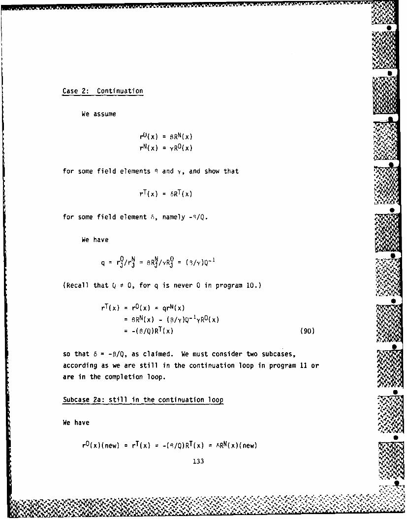
I0

S

Case 2: Continuation

We assume

rO(x) = SRN(x)

rN(x) = yRO(x)

for some field elements 9 and Y, and show that

rT(x) = 6RT(x)

for some field element 6, namely -P/Q.

We have

O N NOq = rj/rj = 9Rj/yRj = (9/y)Q-i

(Recall that Q # 0, for q is never 0 in program 10.)

rT(x) = r0(x) = qrN(x)

= BRN(x) - (0/y)Q-'yRO(x)

= -(B/Q)RT(x) (90)

so that 6 = -0/Q, as claimed. We must consider two subcases,

according as we are still in the continuation loop in program 11 or

are in the completion loop.

SSubcase 2a: still in the continuation loop

We have

r0 (x)(new) = rT(x) = "(9/Q)RT(x) ARN(x)(new)

133

and .-,

rN(x)(new) = xrN(x)(old) = YxRO(x)(old) = yRO(x)(new),

satisfying the conditions assumed for conclusion of a continuation

loop.

Subcase 2b: in the completion loop

We have

rO(x)(new) = xrN(x)(old) = yxRO(x)(old) = yRO(x)(new) 0

rN(x)(new) = rT(x) = -(q/Q)RT(x) = 6RN(x)

satisfying the conditions assumed for conclusion of a completion

loop. •

Since initially the programs begin with

r0lx) = ROx)

and

rN(x) = RN(x)

the assumptions for both case 1 and case 2 are always met. Thus, at

every iteration j the polynomials aJ(x), bJ(x), and rJ(x)

produced by program 11 differ from those produced by program 12 only

by a scale factor (though of coursa the roles of r0(x) and

rN(x), etc., are sometimes reversed).

134

I S

%

We have now shown that program 5 (Mills' algorithm) is

equivalent to program 11, which is equivalent to program 12, which

is equivalent to program 8, which in turn is equivalent to program

7, which is an expanded version of program 6 (Berlekamp's

algorithm).

A

We conclude that Mills' algorithm and the Berlekamp-Massey

alyorithm may be viewed as variants of Euclid's algorithm which are

equivalent in the sense that partial results produced by one

algorithm can be mapped directly into partial results produced by

the other.S

To complete this section we display table 2 showing the

polynomials rT(x) and RT(x) defined at each iteration j for

examples 16 and 17 using programs 11 and 12, respectively. Also

shown are the values of the polynomials rO(x), rN(x), RO(x),

and RW(x) at the beginning of the iteration (i.e., these are the

values determined for these polynomials during the j-ist

iteration). From the table it is readily observed that the

relations (89) and (90) hold for rT(x) and RT(x) determined at

iterations following execution of a completion loop and following

execution of the continuation loop, respectively.

%*%

135

Z' a. %'-

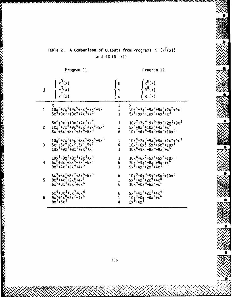
Table 2. A Comparison of Outputs from Programs 9 (rT(x))

and 10 (RT(x) )

Program 11 Program 12

0 0

r (x) 0R (x)

Ir (x) R T N(x)

x 6 5 4 3 21 x 6 5 4 3 210lx +7x +9x +8x +2x +9X 1 lox +7x +9x +8x +2x +9x

5x 6+9X5 +lox 4 4x 3+X2 1 5x 6+9x 5 +lOx+4x 3+X2

5x 6+9x 5+lox 4+4x 3+X2 1 lox 7+7x 6+9x 5+8X4 +2x 3+9x 2

2 1017 +7 -6+9X5 +8X4 +2X3+9X2 1 5x 6+9X5 +lox 4 +4x3 +X25x +3x +8x 5+3x 4 +5x 3 6 lox 7+6x 6+5x 5+6x4 +lox 3

1OXB+7x 7+9x 6+8x 5+2 X4+9X 3 1 lox 8+7x 7+9x6 +8x 5+2x 4+9x 3

3 5x 7+3x 6+8X 5+3X4~ +5x 3 6 lox 7+6x 6+5x 5+6x 4+10X3lox 8+9x 7+8X 6+9x 5+X 4 1 lox 9+9X 7+8X 6+9x5+x4

1Ox8+9x 7+8x 6+9X 5+X4 1 lox 8+6x 7+5x 6+6x 5+10X4

4 5x 8+3x 7+8x 6+3x 5+5X4 6 1OXB+9x 7+8x 6+9x 5+X49x8+4x 7+2x 6+4x 5 1 9x 8+4x 7+2x 6+4x 5

5x 9+3x 8+8X 7+3x.6 +50 6 lox 9+6x 8+5x 7+6x 6+lox 55 9x 8+4x 7+2x 6+4x 5 1 9X 8+4x 7+2x 6+4x3

5x9+0x8+3 X7+bX6 6 lox 9+Ox 8+bX 7+X6

5x 9+Ox 8+3x 7 +6X6 6 9X 9+4x 8+2x 7+4x 66 9x 9+4x 8+2x 7+4x 6 1 lox 9+Ox 8+6x 7+X6

8x 9+5x 8 4 2x 9+4x 8

136

%.-. . . . . . .

WWI~~. W. N.,l Iv

7.5 COMPARISONS .. %

In this section some comparisons are made among the various

algorithms which have been treated so far. We first compare,

briefly, the versions of the Berlekamp-Massey algorithm that have

been discussed; second, we make comparisons among the different

versions of the Euclidean algorithm; finally, we make comparisons

between the two classes and consider whether there is any choice to -

be made between programs 8 and 12.

The three versions of the Berlekamp-Massey algorithm which have

been discussed are represented by programs 6, 7, and 8. All three

programs solve the key equation (14) for k(x); programs 7 and 8 also

provide (x) at the cost of more multiplications and storage for

a(x). Program 6 requires computation of the discrepancy d at every

iteration by a vector inner product calculation whose length grows

at each iteration. This would be highly undesirable if the

algorithm were to be implemented in a VLSI systolic array. Programs

7 and 8 avoid this calculation by retaining, instead, an additional

trio of polynomials rN(x), rO(x), and rT(x).

Program 8 is more efficient than program 7 in that the updates

of the old polynomials rO(x), a0 (x), b0 (x) in lines 15-17 do .

not require a multiplication. However, both programs may be

unsuitable for VLSI implementation. Program 7 usually requires .

computation of a finite field inverse d-1 at alternate iterations,N 0 .- ""<

while program 8 requires a finite field division rj/rj at every

iteration. Both operations are considered difficult to implement in

VLSI. In section 8.1 we examine Burton's enhancement of the

Berlekamp-Massey algorithm. This modification obviates the need for

computing finite field inverses or performing finite field division

137

J. % % .w~I% ~ ~ -- :

within the Berlekamp-assey algorithm. (Of course, a division is__

still required outside the algorithm if Forney's formula (16) is

used to calculate the error magnitudes.)

The Euclidean decoding algorithms under consideration are

represented by programs 4, 5, 11, and 12. It is clear that programsanalogous to 11 and 12 can be constructed for the Japanese algorithmof program 4. Both programs 4 and 5 suffer certain deficienciesco lmpared to programs 11 and 1 an th Be l k -Massey programs: P

they require polynomial division, itself an iterative algorithm.; incertain situations they can have problems with termination; and _wthere is a constant irksome need to determine the degrees of, . %polynomials and vary action accordingly. '

The quotient polynomials q(x) in programs 4 and 5 are usually,7though not always, linear. On the average, one polynomial division %of the Euclidean algorithm is equated with two iterations of theBerlekamp-Mlassey algorithm. But when we break the polynomial' r....edivision of Mlills' algorithm down in to its component partial -€

divisions in program 11, the number of iterations becomes 2t for ._both algorithms. The difference is that each pair of iterations in 'Zthe Berlekamp-Massey algorithm consists of two nearly identicalsteps, whereas each pair of partial divisions in the Japanese or 'w

Mills' algorithms consists of two distinct steps, clearly favoring "°... ,t h e f o r mn e r ..

, .

• ~.. . -- .

Termination in programs 4 and 5 is correctly determined if the .. .

number of errors does not exceed t, the underlying assumption. .However, in the b~erlekamp-Massey algorithm, if more than t errors .. ,?have occurred, the length X of the shift-register will sometimes, -.-

Z .

VF %

*1 1v.P138.p~

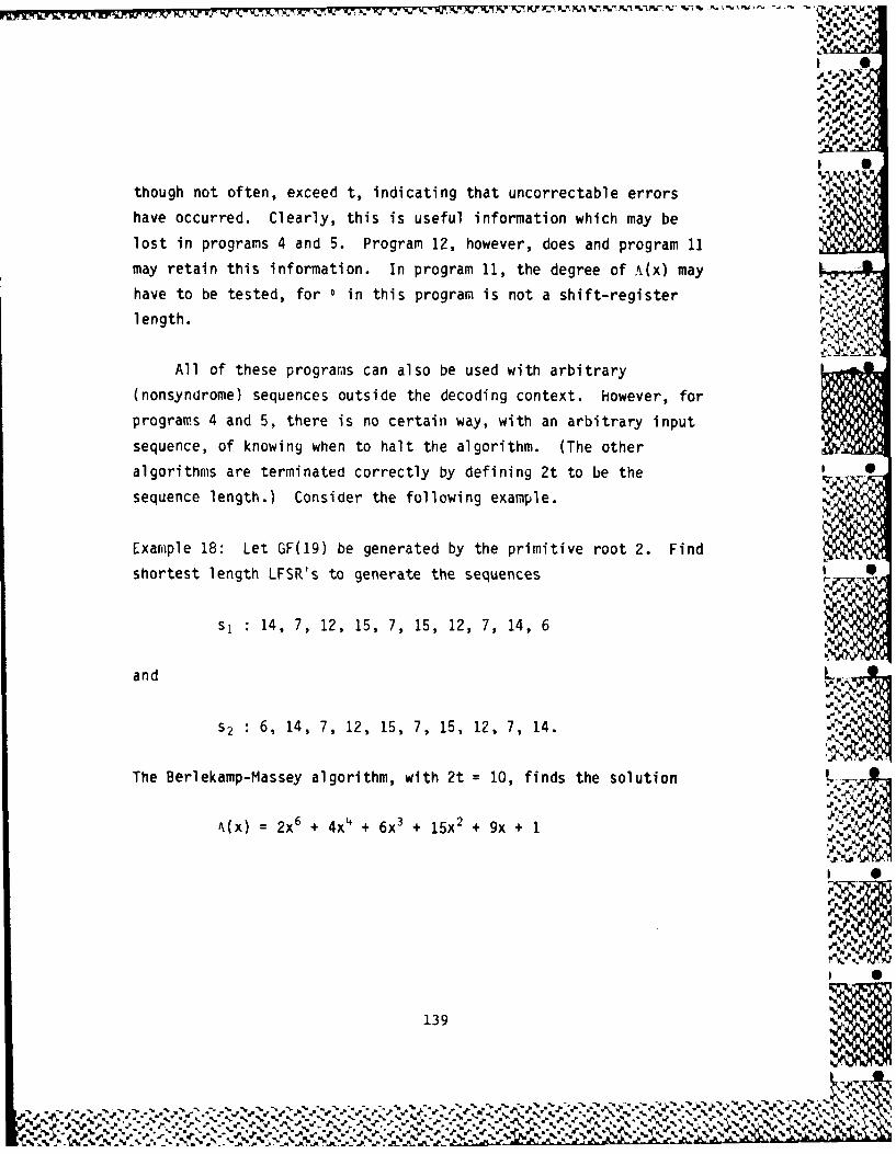
WU7 KIM? VJ KIT. '' ~ ~ ~ ~~

though not often, exceed t, indicating that uncorrectable errors

have occurred. Clearly, this is useful information which may be

lost in programs 4 and 5. Program 12, however, does and program 11

may retain this information. In program 11, the degree of A(x) may

have to be tested, for 0 in this program is not a shift-register-.>

length.

All of these programs can also be used with arbitrary

(nonsyndrome) sequences outside the decoding context. However, for

programs 4 and 5, there is no certain way, with an arbitrary input

sequence, of knowing when to halt the algorithm. (The other

algorithms are terminated correctly by defining 2t to be the

sequence length.) Consider the following example.

Example 18: Let GF(19) be generated by the primitive root 2. Find

shortest length LFSR's to generate the sequences 5

s, : 14, 7, 12, 15, 7, 15, 12, 7, 14, 6

and L

NS2 6, 14, 7, 12, 15, 7, 15, 12, 7, 14. .

The Berlekamp-Massey algorithm, with 2t 1 10, finds the solution

&Wx) 2x6 + 4x4 + 6x3 + 15x 2 + 9x + 1

"

139

% %- % % % %,

for sequence sl. Programs 11 and 12, with 2t = 10, find scalar

multiples of this same solution: 7

14f(x) = 9X6 + 18X 4 + 8x3 + X2 + 12x + 14.

and

3A(x) = 6x6 + 12x4 + 18x3 + 7x2 + 8x + 3. 0

However, programs 4 and 5, with t = 5, terminate too soon with the

polynomial

b(x) = 15xL + 2x3 + 16x 2 + 2x + 15. - . -

If allowed to continue for one more iteration (e.g., by setting

t = 6) both programs find a correct (though different) solution.

When the reversal input sequence S2 is used, both programs 4

and 5 terminate correctly if t is chosen to be 5, but produce an

incorrect result if t is set equal to 6. Thus, there is no safe way

to use these programs with an arbitrary input sequence. (The

programs terminate correctly if the sequence is repeated once and t

is taken to be its original length 10.) Programs 8 and 12 have no

difficulty with sequence s2 . _

" -. '1%

The third objection to programs 4 and 5 is the constant need

for determining the degrees of the polynomials used in the . ..... '9algorithms, and for varying the action taken accordingly. Such a

determination and comparison is implicit in each execution of (84).

140

I" .- " w ,; "',% , ,,'.. .- '.- .. .:.-..' .-.... .. ,- .' .".";% * "'~'.. "

- % .. /5 " " . "% ''. .%. 5,. ... , . -,

When used to find a minimum length LFSR which generates an

arbitrary sequence, even program 11 can have a problem, at ".

termination, in determining the correct degree of the shift-register

polynomial. (Recall that 9 in program 11 does n 't denote the

shift-register length.) A correct solution for the sequence S2 of

example 18 is

A(x) = Ox5 + x4 + 9x3 + 15x 2 + 9x + I.

The proper shift-register length is 5, not 4, that is, the last

stage must be included even though it is not tapped. Program 11

finds a correct shift-register connection polynomial (a scalar •

multiple of f(x)), but is unable to tell the correct shift-register

length. -C

We conclude that for three substantial reasons, programs 4 and

5 are not competitive with programs 7, 8, and 12. Program 11 also

seems to be out of contention; there is no reason to execute two

distinct equally complex loops instead of executing one of them

twice. Thus, we are left with comparing programs 8 and 12.

Between these two programs there would seem to be no

preference. Both have the flaw that a finite field division is ,

required. This we remove in section 8 by applying Burton's S

innovation. Program 8 produces a monic error locator polynomial

A(x). This may possibly give some advantage to program 8, depending

on the method chosen to complete the error correction. However, as -

we have seen, neither the Chien search nor Forney's formula (16) 0

%,..141,

7 % %

benefits from the use of a monic error locator polynomial.

Furthermore, incorporation of Burton's enhancement eliminates the

monicity advantage, if there is one.

Table 3 summarizes the estimates of the number of

multiplications required for each of the programs. All basically

require on the order of 4t2 multiplications to find A(x) when t

errors have occurred. Program 6 can get by with 2t2 multiplications

if bO(x) is not normalized, but does not provide r(x), and

involves an unacceptable delay in the computation of the

discrepancies. Program 7 becomes program 8 when the normalization

of bO(x), aO(x), and rO(x) is omitted. All programs except 0

program 6 require 2t basic time units for correction of t errors,

where a basic time unit includes the time required for a finite

field division (or inversion), a multiplication, and a subtraction.

Table 3. Number of Multiplications Required

for Obtaining k(x) in the Presence of t Errors

Program Number of Multiplications Remarks

4 4t2

5 5t2 16 2.5t 2 27 6t 2

8 4t 2

11 4t2

12 4t2

1 can be reduced to 4t2 by dropping terms from r(x)

2 can be reduced to 2t2 by omitting normalization of bO(x)

142

,% % % % % I

, •\

SECTION 8

INVERSIONLESS DECODING

All programs which have been considered so far require

inversion of finite field elements or, equivalently, division of

finite field elements. These operations are generally considered to

be difficult to implement efficiently in VLSI. In this section we S

consider algorithm modifications which avoid explicit computation of

inverses ana division at the cost of further multiplications. In

section 8.1 we examine Burton's [27] inversionless variant of the

Berlekamp-Massey algorithm,. In section 8.2 we look at analogous S

methods for avoiding the computation of inverses in the Euclidean

decoding algorithms.

8.1 BURTON'S ALGORITHM •

Burton [27] has given a modification to Berlekamp's algorithm

which eliminates the usual inversion of the discrepancy d at each

iteration, or, equivalently, the division r /r8 at each S

iteration in Citron's version (program 8).

At line 11 of the recursion in program 8 we want to compute the

new shift register polynomial by -

bTW b rr/r 9 lbO(x) (91)

143

*'P

START

0 ph0 b0(x) - xbO(x)

-0 a0(x) - x80(x)

&'(X) - 1 Ox -xOx

rr(x) - JcSfx) b N(X) - bT(x)0

so (x) - - 1 a N(X) - uT(X)

aT(X) -0 rN(x) - rT(X)

bT(x)1 2t >EXIT

b T(X) - lbaN(X) - rf'a0(x)%

arT(X) - IJaN(X) - ,4 0(X)

b0(x) b bN(X)

80(X) - aN(X) ,

r0(x) - r"(X)

RECURSION

INPUT: SYNDROME POLYNOMIAL S(x), INTEGERt

OUTPUT: A(X) b bN(X), 9,f(X) = aN(X)IX

Program 13. BURTON'S ALGORITHM

144

AeV

V~

% %*

without having to divide. Multiplying (91) by r gives

r 0 b T W = &'b(x) - r'b (x).

Burton accepts rjbT(x) as the new shift register polynomial in

place of bT(x) as defined by (91), and similarly for aT(x) and

rT(x), giving program 13. At the termination of program 13 we end

up with a2t(x)/x = yQ(x) and b2t(x) = yA(x) for some nonzero

field element y. This is acceptable, since neither the Chien search

for the error locations nor Forney's calculation of the error

magnitudes is affected. Citron [22] has also used Burton's L

modification to obtain an inversionless algorithm equivalent to

program 13.

Example 19: Reed-Solomon 3-error-correcting code over GF(11) with

=2. 4

t =3; Let c(x) = 0, v(x) = e(x) =6x + 5x8 + 3x.

S(x) = lOx 5 + 7X4 + 9X3 + 8x2 + 2x + 9

S0, 9 =0

rN(x) = xS(x) = 1OX6 + 7x' + 9X4 + 8X3 + 2X2 + 9xrO(x) = xbN(x) = 1

bO(x) = 0

aN(x) = 0

aO(x) = -x = lOx

N

145

. . . . . . . . . . . . . . .. . . . . . . . . . . .. ... i : - .

- - % %-"

j =1, . =0: r. 9, ry= 1

rN(x) '- rh(x) - 9r0(x) = lOx6 + 7x5 + 9X4 + 8,0 + 2xr0(x) +- xrN(x) = lOX7 + 7X6 + 95+ 8X4 + 2X3 + 9X2

bN(x) -bN(x) - 9b0(x) = 1b0(x) +- xbN(x) = x

aN(x) +- aN(X) - 9a0(x) = 9xa0(x) +- xaN(x) = 0

2, =1: r. 2, r.= 9

rM(x) -901k~) -2r0(x) =2,0+lx 0' + 203

r0(x) -xr 0(x) =lOxb + 7x7 + 9x6 + Wx + 2X4~ + 9X3

bN(x) 4- 9bN(x) -2b0(x) = 9x + 9

b0(x) 4- xb0(x) =X 2

aN~(x) +- 9aN(x) -2a0(x) = U4IxL

aolx) 4- xa3(x) U )

j 3, 9.=1: r. 2, r9= 9

rN(x) +- 9rN(x) - 2r0(x) =2x8+ 4X7 + 6x6 + 45~ + 9x 4

r0(x) +- xrN(x) =2x' + l~7 +x ~ + 2xbtJ(x) ,- 9bN(x) -2b

0(x) = 9X2 + 4U + 4b0(x) '- xbN(x) 9X2, + 9XaN(x) +9aN(x) -2a

0(x) =3xa0(x) +xaN(x) =4X2

%

146%

%~ %

4,. =2: r N 9, r0 2

vrN(x) -2rl4(x) - 9r0 (x) =8X8 + 6X7 + 3X6 + 6W

r0(x) 4- xrN(x) =2x' + lOX8 + X7 + lOX6 + 2xbbN(x) -2bN(x) -9b

0(x) = 3X2 + Ux + 8b0(x) 4-xb

0 (x) =9X3 + 9X2

aN(x) 4-2aN(x) -9a0(x) =8X2 + 6x

a0(x) 4-xa 0(x) =4X 3

j=5, ~.=2: r.=6, 0= 2

rN(x) 4- 2rN1(x) -6r0(x) =lOx

9 + Ox + 6X7 +X 6 9rO(x) .- xrN(x) W , + 6x' + 3, + 6x'bN(x) 4- 2bt4(x) -6b 0(x) = X3 + 7X2 + 8X + 5b0(x) 4- xbN(x) =3X

3 + 4X2 + 8xaN~(x) 4- 2aN(x) -6a

0(x) = 9X3 + 5X2 + Xa0(x) +- xaN~(x) =8X3 + 6, X2

j=6, Q.=3: r 1, r0= 6

rN(x) *-6rN(x) - rO(x) W x + Sxb + Ox7

r0(x) 4- xr0(x) 8 x" + 6x X + 3x X + 6x7

bN(x) 4- 6bN(x) -b 0(x) = 3 + 5x + 7x +8b0(x) 4-xbO(x) =3x' + 4X3 + 8X2

aN(x) ~-6aN(x) -a0 (x) = 2X3 + 2X2 + 6x

a0(x) 4-xa 0(x) =8 4 + 6x.' .

147 I.%Zp-

j = 7, stop. Y = 8, y- 1 7

&(x) = y-ibN(x) = lOx 3 + 2x2 + 5x + 1e(X) = y-laN(x)/x = 3x2 + 3x + 9

x2 tA(x) = y-'rN(x)/x = x8 + 2x7

AW = x 2 + 2x

Burton's modification almost doubles the number of

multiplications. We require 4t2 + 2t multiplications to update

rT(x), 2t2 + 2t for bT(x), and 2t2 - 2t + 2 for aT(x) for a

total on the oraer of bt2 multiplications.

8.2 INVERSIONLESS EUCLIDEAN ALGORITHMS S

The Japanese decoding algorithm and Mills' algorithm can be put

into inversionless form by Burton's technique if we first break the

polynomial divisions down explicitly into their partial divisions

as was done in program 11. To eliminate the finite field division

in the completion loop of program 11, we delete statement 10 (which

defined q) and replace statement 11 by

bT NO0 ON~(x) rb W(x) - r~b (x) (92)

etc., resulting in program 14. Sugiyama, et al. [12) have used

Burton's technique to yield an inversionless variant of their

algorithm which is equivalent to program 14. Program 14 requires on

the order of 8t2 multiplications. Shao, et al. [28] have also

presented an inversionless variant of the Japanese algorithm which

is similar to program 14.

148

-AL-

w ,i -~,'. ' . ', W '- i , " -w -- ' ._W- '-r

- . ,', "• " -" "% ,',"'"-. ."-"". ."" ." •."'-. .%-" .%

0 pb*X - xb~)b~x T

j 8 0 x) - X 8 0( ) 8 0 X) - 8 T'X

0SX bN(X) - b0() bllfx) - xb(x)

80(X) 1r() - aN(X ) 0() - rTx)rT~x KS~) bNx) -bT) - Xb"(X)BT(x) - 0 rN(X) - rT(X) aN(X) - XSN(X)

b0(x) -0 j - i f (+br(X) H 2t:t

INTAIZTOo CONTINUATION LOOP

bT(X) _rl'bOx) - &j bN(X)

aT~) ra0() -r8N(X) EXITrT(X) - r,"rO(X) FQ~"(x .-

b0(x) - bN(X)

a0(x) -aN(X)

COMPLETION LOOP

INPUT: SYNDROME POLYNOMIAL S(x), INTEGER tOUTPUT: I, X(x) =bN(x), Q f(x) =aNl(x)Jx

Program 14. INVERSIONLESS MILLS' ALGORITHM

149

I

Finally, let us apply Burton's technique to the simplified

Mill's decoder of program 12. Analogous to the changes made in

program 8 to obtain program 13, we delete statement 10 of the

recursion which defined q, and modify statements 11-13, replacing -

statement 11 by (92), etc., as in program 14. These changes produce

program 15. It is manifest that programs 13 and 15 are equivalent,

the only difference being the signs of the r.h.s. of statements

10-12 of the recursion. Example 20 shows how this change affects

the partial results.

Example 20: Reea-Solomon 3-error-correcting code over GF(11) with

=2.

t = 3; Let c(x) = 0, v(x) = e(x) = 6x9 + 5x8 + 3x.

S(x) = lOx 5 + 7x4 + 9x3 + 8x2 + 2x + 9.

j=0, 9=0

rN(x) = XS(x) = x + 7 + 9x4 + 8x0 + 2 + 9X

rO(x) = xbN(x) = 1

bO(x) =0aJ(x ;) = 0

aO (x) = -x = lOx

j = 1, 0 =: N = 9, r = 1

rN(x) + 9rO(x) rN(x) = X6 + 4X5 + 2x4 + 3X3 + 9X2

rO(x) + xrN(x) = lOx 7 + 7x6 + 9x 5 + 8x 4 + 2x3 + 9x 2

bN(x) - 9bO(x)- bk(x) = 10

bO(x) + xbN(x) = x .

aN(x) + 9aO(x) aN(x) = 2x .aO(x) - xaN(x) = 0

, 5

150 UN I

START

0 b0(x) - xb0(x)o 80(x) - Xa0(x)

10(x) - 1 r0(x) - x0(x)

rT(x) .- xS(x) bN(x) - bT(X)

80(x) - - 1 IN(X) - aT(X)agT(X) -0 rN(x) - rT(X)

b(x -O0 j-+1

bT(X)1 j:2t > EXIT0

T(K rrf ~ ) r:0x

INITIALIZATION %Tx -rb() ~Nx .~

aT(X) -rNa()- ONx

rT(x) .- 4(X) - rjor"(x)

b0(x) -bN(x) '

r0(x) -rN(x)

RECURSION .41-f

INPUT: SYNDROME POLYNOMIAL S(x), INTEGERt

OUTPUT: ,A(X) =bN(X), I 9l(X) = aN(X)j 1

Figure 15. BURTONIZED MILLS' ALGORITHM - FINAL VERSION

151

% % % P~~'~~~s~~'~~t- A-'j~.'p~..,'s".

~%

j 2, =1: r.N 9, r? 9

rN(x) ~- 9r0(x) -9rN(x) = 2X7 + lOX6 + X5 + lOX4 + 2x'r0(x) 4- xr0(x) =lOx 8 + 7x +9x + 8x + 2x +9x

bt1(x) ,9b 0(x) -9bN(x) = 9x + 9 .

b0(x) +- xb0(x) =X 2

aN(x) +- 9a0(x) -9aN(x) = Ux

a0(x) +- xa0(x) =0

j=3, 2=1: rN= 2, 0= 9

r1N(x) <- 2r0(x) -9rN(x) = 9x8 + 7 X7 + 5x6 + 705 + 2X4 .

r0(x) 4-xrN(x) =2x8 + l~7 +x ~ 5 + 2x

btN(x) 4-2b0(x) -9bN(x) = 2X2 + 7x + 7

b0(x) 4- xb14(x) =9X2 + 9X

aN(x) 4- 2a0(x) -9aN(x) =8x

+Ox - =a~x 4X2

N 04, 2:r i 2, i =

rN(x) 4- 2r0(x) - 2rN(x) W x + 6X7 + 3X6 + 6x 5

rO(x) - xrO(x) =2x9 + lOX 8 + X? + lOx 6 + 2X5

bN(x) 4- 2b0(x) -2bN(x) = 3X2 + Ux + 8b0(x) 4- xb0(x) =9X 3 + 9x 2

aN(x) +- 2a0(x) -2aN(x) =8X2 + 6x

a0(x) +- xa0(x) =4X 3 .4

fl 0

152

.............----

j=5, 9 2: =6, r9 2

rN(x) - 6r0(x) - 2rN(x) =X9 + Ox 8 + 5x 7 + lox 6

r0(x) 4- xrN(x) 8W + 6xp + 3X7 + 6X6

bN(x) -6b0(x) -2bN(x) = lOx 3 + X2 +3

b0(x) -xbN(x) 3X3 + 4X2 + 8x +4 +3

ANx) 4- 6a0(x) -2aN(x) = 2X3 + 6X2 + lOxa0(x) -xaN(x) 8X3 + 6X2

=6, ~'=3: r.=10, r.= 6

rN(x) 4- 10r0(x) - 6r1N(x) =x9 + 5xa + Ox7

-

r0(x) 4- xrO(x) 8X1 + 69+ -'X8 + 6x7bN(x) . lb 0(x) -bbN(x) = 3x3 + 5A 2 + 7x +8bO(x) 4- xb0(x) =3x' + 4x0 + 8xIaN(x) ~- 10a0(x) -6aN(x) = 2x3 + 2X2 + 6x

a(I.Xao(X) g X4 + 6X3

j=7, stop. y=8, y'=7 '

k(x) = v-'bN(x) = lOx3 + 2X2 + 5x +1.-()= Y'latl(x)/x = 3X2 +3x + 9

xt1(x = Y-'rN(x)/x = xS x?(X = 2+ 2x

153

% A

7 177

r

SECTION 9

DECODING ERASURES

In this section earlier results are extended to include the

decoding of erasures in addition to errors, where an erasure is an

error whose location is already known to the decoder. A BCH t-error

correcting code, with minimum distance 2t + 1, is capable of S

correcting any combination of v errors and 4 erasures for which

2v + p < 2t. Forney [9] first showea that by employing modified

syndromes one can still solve for the error locator polynomial in .

the presence of erasures. Blahut [29] showed that the errata 0

locator polynomial (where an erratum is either an error or an

erasure) can be calculated directly (without first finding the error

locator polynomial) by initializing Berlekamp's algorithm with the

erasure locator polynomial. In this section we combine these S

results to give a program which provides both the errata locator

polynomial and the errata evaluator polynomial. Errata magnitudes

can then be calculated by Forney's formula (16) or by the new

formula (24). 0

As in section 3, we assume a BCH code designed to correct t

errors in a codeword of length n = - 1 for q a power of a

prime. Let c(x) represent the transmitted codeword polynomial and 5

e(x) be an error polynomial. In addition, let d(x) represent the

channel erasure polynomial. The received codeword polynomial is now

v(x) = c(x) + d(x) + e(x).-

155

NO % % % % -•.,-

% le-" AZ'

We define 2t error syndromes by p.

Si = v(ai) = c(aj ) + d(qj) + e("j)-

= d(aj) + e(aj) (j = i, ... , 2t)

where a is a primitive element of GF(qm).

Suppose v errors and u erasures, where 2v + < 2t, have

occurred during transmission. We define v unknown error locations

X9, where Xo is the field element of GF(qm) associated with

the 9th error location, and N) unknown error magnitudes Yz, where

Y, > 0 and Yz c GF(q). In addition, we now define u known era-

sure locations Wk E GF(qm), where Wk is the field element

associated with the kth erasure location, and 4 unknown erasure

magnitudes Vk E GF(q). The Wk are always assumed to be distinct

from the Xz. Vk is the difference between the transmitted

symbol at location Wk and the symbol assumed for the kth erasure Ile

at the receiving end. Unlike YR, Vk may assume the value 0.

The 2t syndromes are now given by the 2t BCH decoding equations

S. = e("A + d(',3) Y X + Vk kk=k.1 k l 1

= E. + Di. (j = 1, ... , 2t). (93) A

4,.'% .W

156%- %

The error-and-erasure decoding problem for BCH codes is to solve

this set of 2t (nonlinear simultaneous) equations for the v unknown

error locations Xv, the v unknown error magnitudes Yj, and the t

unknown erasure magnitudes Vk, given the 2t syndromes Sj and the

p erasure locations Wk. Forney's solution is to derive from the

set of 2t equations (93) a reduced set of 2t - u equations of the

form (9) which can be solved for the error locator polynomial A(x).

If we define '(x) by (10), and Ej by .

E. = ? YXj, = 1, 2t)

then by a process identical to that which obtained equation (11)

from (10) in section 3, we arrive at A L

VS

0 +vi' 1= , 2t). (94)

This set of 2t simultaneous li,,ear equations could be solved to

obtain x) if we knew the Ej. However, we do not know the Ej,

but only the Sj =Ej + Dj, where

57

V-VW.

k% k

We now define the erasure locator polynomial as the monic -I

polynomial having zeros at the inverse erasure locations Wk for

k = 1, ...,

• (95) "" 'J< q s.. ' ',

x) = (1 - WkX) 1 + ix (95)k=1l i = 1- ,.

L. ki 2.1

(If ,i 0, K(x) is defined as the zero-degree polynomial 1.) Forney

uses the erasure locator polynomial <(x) to define a set of 2t -

modified syndromies Tj (j = ,. + 1, ... , 2t) and to derive a reduced

set of 2t - k equations froi (94) in the modified syndromes Tj

which can be solved for A(x). -- '--

Let the modified syndromes be defined by

Tj i=K i Sj + 1, 2t). (96)i". .

By extension, defining Sj = 0 for j outside the range (1, 2t)

allows (96) to be used for defining Tj for j outside the range "JV .;"*- '

(G + 1, 2t).

Now, since Wk-1 is a zero of i(x) for k = 1, ... , ±, we have

Ki 0=, 0--,_V --

i o=0 ; .*.{*

and -r

Y . L * i = 0 . V ,. V ..i:0 '- J - -

158

~ , ~

"A MR -k-wVrw it " rS

Therefore,

T. = KS. = Y .(E. + D. . \' .E.. (97) :~3 - J 1 0 i J-1

1=0 101 i=0 3

We now multiply (94) by K,~ and sum a± + 1 successive equations, .

using (97) to obtain the set of 2t - a equations __

V0

0; j+v-z+ i= 1 AjJ 4 1

T. + Y A.T. j (j = + 1, .. 2t). (98)

This set of 2t - iL equations in v unknowns ki, where 2v < 2t -iis exactly analogous to the set (11), and can be solved for A(x) byP0the Peterson-Gorenstein-Zierler algorithm exactly as in section 3.

The modified syndrome polynomial is defined analogously to S(x)by

2tT~)= j ~~ (99)

j=i

=IK(X)s(x)I X2t

and the errata locator polynomial 11(x) is defined as the product ofthe erasure locator polynomial and the error locator polynomial:

lix) = '.x)h(x). (100)

159..

,Il

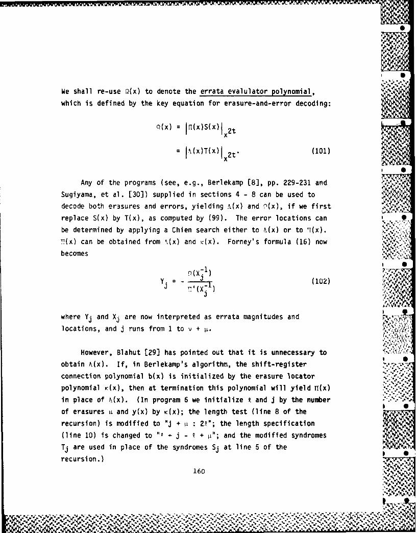
We shall re-use Q(x) to denote the errata evalulator polynomial,

which is defined by the key equation for erasure-and-error decoding:

Q(X) = INxIS(I x2t

= Ix(x)T(x)I x2t (101)

Any of the programs (see, e.g., Berlekamp [8], pp. 229-231 and

Sugiyama, et al. [30]) supplied in sections 4 - 8 can be used to

decode both erasures and errors, yielding A(x) and nx), if we first

replace S(x) by T(x), as computed by (99). The error locations can .

be determined by applying a Chien search either to &(x) or to i(x).

N(x) can be obtained from k(x) and K(x). Forney's formula (16) now

becomes

ix 1 I

Y -- (102) i .e I

(x"

where Yj and Xj are now interpreted as errata magnitudes and

locations, and j runs from 1 to v + '. ".

However, Blahut [29) has pointed out that it is unnecessary to "V:,

obtain A(x). If, in Berlekamp's algorithm, the shift-register . .

connection polynomial b(x) is initialized by the erasure locator

polynomial K(x), then at termination this polynomial will yield rI(x) ,

in place of f(x). (In program 6 we initialize t and j by the number

of erasures u and y(x) by d(x); the length test (line 8 of the

recursion) is modified to "j + u : 2"; the length specification

(line 10) is changed to ,,0 j - + ii"; and the modified syndromes

Tj are used in place of the syndromes Sj at line 5 of the

recursion.) V 6l

160 % p

% - -A - w .J " ..! .%,

If we use one of the Euclideanized versions of the Berlekamp-

Massey algorithm, we directly obtain the errata evaluator polynomial

o(x) as well as '1(x). We show this in program 16, which is program

13 (Burton's algorithm) modified for handling erasures, and with

a(x) superimposed on r(x). In this program the integer a represents ,

the number of erasures. If = 0, the program functions like

program 13. There is no confusion in superimposing aN(x) and

rN(x), since at iteration j, ri = 0 for i < j, 9 < j, and by 0

(66) a4 = U for i > z. When u > 0, r lmy be nonzero for i <

at iteration j > a, but af = 0, so there is no problem in

determining r.

There is a problem with r0(x), however. Note that r0(x) is

now initialized by U, the sum of the initializations for aO(x) and

r0(x) in program 13, but we still need rO(x) = 1 for the initial

update of rT(x). Therefore, following Burton L27], we retain an

additional variable 6 to represent the ola discrepancy value. This

is initialized as 1 and updated as the current discrepancy d at

every length change. The variable 6 is not needed if a(x) and r(x)

are not superimposed.

At termination we have

rN(x) = aN(x)(-l) + bN(x)xS(x).

For bN(x) to give Yr(X), we must have, by (101),

yQ(x) = 1(aNlx) + rN(x))/x2t

thus providing the motivation for superimposing the two polynomials.

161

' o r -r . .rV- .

START-

1 r0(x) - xr0(x)rowx - 0 bOx) - xb0(x)

b 0 (x) - 0r'(x) - rT(x)rT W) - xS(x) bN(x) - bT(x)-

.A

bT(X - 1 1-j1+11 0 j: 2t EXIT

j1 j+1 d :0rT() ( i)r T(X) rT(X) .- 6"N(x) - dr0(x)

bT(X) -(1 - Wix) bT(X) bT(x) - bN(X) - dbOx)

1 + u 2fINITIALIZATION r0(x) -r 4(x) O

b0(x) 4-bN(X)

RECURSION

INPUT: SYNDROME POLYNOMIAL S(x), ERASURE LOCATIONS W, (FIELD ELEMENTS)NUMBER OF ERASURES u, INTEGERt

OUTPUT: jfl(x) =bN(x), yOQ(x) =Ir'N(x)/xl;2, rI

Program 16. DECODING WITH ERASURES

162

I% % %

%~~I %~ %N'.-

If AW is deie analogously tov- (19)1C byW ,

sueifposed is defined 1 analogouly to (19)/tj byro

magnitudes can then be calculated by a revised version of (24): S

Y. X. -. (104)

where n is the codeword length and d is the designed distance of the

code.

For an example we again call upon the Reed-Solomon

3-error-correcting code over GF(11) with a =2.

No'

%A P

Example 21: Reed-Soloman 3-error-correcting code over GF(11) with

a =2

t 3; Let c(x) = 0, e(x) =3x0 + 7, d(x) =6x9 + 5x.

v(x) =c(x) + d(x) + e(x) =6x9 + 5x0 + 3x3 + 7

Since v(x) for this example is 7 + v(x) for ex. 3, the Sj for this

example are 7 + Sj for example 3.

S(x) 6x + 3X4~ + 5x3+ 4x 2 + 9x + 5

j=0, Z.= 2, 6 S 1, r0(x) = bO(x) = 0

rT(x) ,4 xS(x) 6X6 + 3x' + 5X4 + 4x' 9X2 +5x

bT(x) ,~ 1

=1: W~j a8 3

rT(x) (13x)rT(x) =**.* 8x +

rli) ,(1-x~r~x)= 9X8 + 8x7 + 3~X6 + 8X5 + Ox4 2X+

8x2 +5x

bT(x) .- (1-3x)bT(x) = 7X8 x + 1

j 3, 2 j 2, 8 1

rN~x) r(x) r(x) = 9x 8 + Ox7 + 3X6 + 8X + lOx4 +20+8x + + 5x

rN(x) .4-rN(x) - r0x) + x7 + 3 + 8 5 + loxx 5 +

2x +9~ 5x

bN(x) .- bN(x) -2b0Ox) = 7, + 2x + 1I' .~

b0(x) .- xbN(x) = 7x + 2x 2 + x

164

.- ,*- .', ~r...t~M~ r *4. .~.;~ ~*~ . ', - .-. * *-.-A. **v*. .

4, . : 3 rN 1 10, 6 = 2

rN(x) + 2rN(x) - lOrO(x) = 9x9 + 7x8 + 3x7 +3x6 + 4x 5 + Ox4 + x3 + lOx 2 + lOx

rO(x) + xrO(x) =9x10 + Ox 9 + 3x8 + 8x7 + lOx 6 +

2x 5 + 8x, + 5bN(x) + 2bN(x) - lObO(x) = 7x3 + 5x2 + 5x + 2bO(x) + xbO(x) = 7x4 + 2X3 + X2

J 5, . : 3 rN : 4, 6 = 2

rN(x) 8x1 o + 7x9 + 2x8 + 7x7 + lox 6 + Ox5 +x + 4x3 + 9x2 + 9x

rO(x) + 9x0 + 7x9 + 3x8 + 3X7 + 4x6 + Ox5 + x4 +lox 3 + 19x 2 •

bN(x) + 5x + 6x + 6x2 + lOx + 4bO(x) + 7x4 + 5x3 + 5;/ + 2x

j = 6, k = 4 = 0, 6 = 4

rN(x) 8x1° + 2x + Ox + 9x7 + Oxb + Ox5 + 5x4 + 4x3 +4-9 8K K

22x2 + 3x % %rO(x) 9x" + 7x" ° + 3x9 + 3x8 + 4x7 + Ox6 + x

5 + %

lOx 4 + lOx3

bN(x) - 5x4 + 7x3 + 7x2 + 9x + 5bO(x) + 7x5 + 5x4 + 5x3 + 2x2

j = 7, stop: y = 5, y- 9

T(x) = y'lbN(x) = x4 + 8x3 + 8x2 + 4x + 1 S

Ox = y IrN(x)/Xl2 t = y- (5x' + 4X2 + 2x + 3)

: x3 + 3x2 + 7x + 5

x2tA(x) y-(rN(x)/x) .'.. *. -.

A(x) = 6x3 + 7x2 + Ox + 4 -.

165

Chien Search: j aJ (J

0 1 01 2 02 4 0 L Ak3 8 3 . .4 5 95 10 9 .

b 9 107 7 0 '- "'.'- '',8 3 8 S9 6 4

Inverse errata locations: a0 a 7 , a2 , a'Errata locations: a0 , a 3 , a 8 a 9

Errata Magnitudes

a) evaluated by Forney's formula (16):

3 2

T'(x) 4x 3 + 2x2 + 5x + 4 . ,

o('zO) 1 + 3 + 7 + 5 5Y1 - -- -____ -- - 7 ,T'(a0) 4+ 2+ 5 +4 4 ,'

( 7 ) 2 + 4 + 5 + 5 5 %Y2 - = - - 3 .,,X .,, ,,:I'(a 7 ) 8 + 10 + 2 + 4 2 ,

Q(a 2 ) 9 + 4 + 6 + 5 2Y3 5

RI(a 2 ) 3 + 10 + 9 + 4 4

Q(a ) 8 1 + 3 + 5 6

r (a1 ) 10 + 8 + 10 + 4 10

I 0

166

%. I S %S .

b) evaluated by the new formula (24):

1(x) = 4x3 + 7x + 6

f(x) = x4 + 4x3 + 8x2 + 8x + 1 .4

W(x) = 4x3 + x + 5x + 8

n - d = (q-1) - (2t+1) = 3

1 ) +4 + 7 + 6 6YI (0) 4 + I + 5 + 8 7 ..- ]

A((T ) 2 + 1 + 6 9 -'Y - -6)"3 = 2 6 - * 6 = 3

FT () 2 + 9 + 7 + 8 4

A( X) 9 + 10 +6 3Y 3 - ,'. 3 : - 5 : * 5 5

('9 +9 +4 +8 8

A(a 9 ) 6 + 9 + 6 10y4 - --- a 9 3 = 7 = - * 7 = 6 S

9i'(a9 ) 6 + 3 + 8 + 8 3-

The loop in the initialization box of program 16, adapted from

Blahut [29], simultaneously computes the erasure locator polynomial

and the modified syndrome polynomial for initializing bT(x) and

rT(x). It is apparent that this loop, or its equivalent, can be

added to the initialization box of any of the decoding programs

discussed earlier for converting them for the handling of erasures.

167

Thus, we can appropriately modify any of these programs to yieldboth lix) and q(x) for error-and-erasure decoding of BCH codes. As

an example we give program 17, which is an adaptation of program 4

for erasure decoding.

In program 17 f(x) is defined as x 2t and g(x) as S(x), sothat at each iteration k we have the relation

rk(xflix 2t = Ibk(x)S(x) I x 2t

holding. In particular, for k = -1, rk(x) = X2t n

bk(x) = U and for k = 0, rk(x) = S(x) and bk(x) = 1. At the

conclusion of the initialization loop rk(x) =T(x) and bk(x)=

K(x). At termination of the program rk(x) Q (x) and bk(x)

7(x), as desired. "eV

Example 22: Reed-Solomon 3-error-correcting code over GF(11) witha2

t = 3; Let c(x) = 0, e(x) = 3x3 + 7, d(x) = 6x9 + 5x.

v(x) = c(x) + d(x) + e(x) = 6x 9 + 5x8 + 3x 3 + 7.

S(x) = 6x 5 + 3X4 + 5x 3 + 4x 2 + 9x + 5

j=0: ro(x) = X2 t, b0(x) = 0 Pi

rN(x) = S(x) =6X5 + 3X4 + 5X3 + 4X2 + 9X + 5

bN(x) = 1

168

~~~~ %. %. %44 %-s~ %~*.. %

*~a -l**

START r(x) 4- ,4 dog (r"(x)) I + A/ <EXIT

bo(x) 4- 0 y(X) - r(x) - q(x)i'4(X)

b"(x) 4- 1 (x) 4- V.

,i N

0 -y(x) 4- bo(x) - q(x)b"(x

j + 1b 0(x) 4- b"(x)

rN(x) (- I (-W x) r'4(x) bNx 4- y ) /

bN(X) 4- (1W~x) N~x)RECURSION

INITIALIZATION

INPUT: POLYNOMIALS x2', S(x); ERASURE LOCATIONS W,NUMBER OF~ ERASURES p. INTEGERt

OUTPUT: rI(x) =bN(x), yO(x) z Nx

PROGRAM 17: JAPANESE ALGORITHM WITH ERASURES

169

%%. -.%,--------------------------------------------------------

j 1: Wi a8 =3

rNW )*I~ xr(x) I ~ 2t= 8x5 + lOX4 +4x + lOx2 + 5x + 5

bN(x) ~-(1 -3x)bN(x) =8x + 1

j=2: Wi a9 =6

rN(x) +I(1 6x)rN(x)I 2 3x 5 + 8X4 + 1OX3 + 2x 2 + 8x + 5

bN(x) ~-(1 -6x)bN(x) =7X2 + 2x + 1 *'

q(x) + rO(x)rNx)J= 4x + 4 .? -

rN(x) +rO(x) - q(x)rN(x) = 5x+ 7x3 + 4U + 3x + 2bN(x) - bO(x) - q(x)bN(x) = 5 + lOx + 7

q(x) ,* LrO(x)/rNx)J = 5x + 10

rN(x) +- rO(x) - q(x)rN(x) = 8x3 + 2x2 + x + 7bN(x) 4- bO(x) - q(x)bN(x) = 8x+ x+9,+ lOx + 8N

deg(rN(x)) =3 < 4 =t + Lp/2j; stop.

y8,y 7

fl~x = 'bN~) = + 8, + 8, + Ux + 1

Q(x) Y yrN(x) =x3 + 3x2 + 7x + 5

170

% -V' %.* %

s~~7.\y

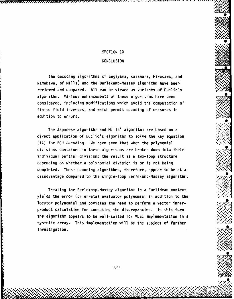
SECTION 10

CONCLUSION

The decoding algorithms of Sugiyama, Kasahara, Hirasawa, and

Namekawa, of Mills: and the Berlekamp-Massey algorithm have been

reviewed and compared. All can be viewed as variants of Euclid's

algorithm. Various enhancements of these algorithms have been

considered, including modifications which avoid the computation oF

finite field inverses, and which permit decoding of erasures in

addition to errors. ,

The Japanese algorithm and Mills' algorithm are based on a

direct application of Euclid's algorithm to solve the key equation

(14) for BCH decoding. We have seen that when the polynomial

divisions containeo in these algorithms are broken down into their .

individual partial divisions the result is a two-loop structure

depending on whether a polynomial division is or is not being

completed. These decoding algorithms, therefore, appear to be at a

disadvantage compared to the single-loop Berlekamp-Massey algorithm.

Treating the Berlekamp-Massey algorithm in a Euclidean context

yields the error (or errata) evaluator polynomial in addition to the

locator polynomial and obviates the need to perform a vector inner-

product calculation for computing the discrepancies. In this form

the algorithm appears to be well-suited for VLSI implementation in a .

systolic array. This implementation will be the subject of further

investigation. -

171 %-....

%171

LIST OF REFERENCES

1. Hocquenghem, A., "Codes Correcteurs d'Erreurs," Chiffres 2(September 1959), pp. 147-156.

2. Bose, R.C. and Ray-Chaudhuri, D.K., "On a Class of ,-.

Error-Correcting Binary Group Codes," Information and Control 3(March 1960), pp. 68-79.

3. Bose, R.C. and Ray-Chaudhuri, D.K., "Further Results onError-Correcting Binary Group Codes," Information and Control 3(September 1960), pp. 279-290.

4. Peterson, W.W., "Encoding and Error-Correcting Procedures forthe Bose-Chaudhuri Codes," IEEE Trans. on Information TheoryIT-6 (September 1960), pp. 459-470.

5. Peterson, W.W., Error-Correcting Codes, The MIT Press,Cambridge (1961).

6. Gorenstein, U. ans Zierler, N., "A Class of Cyclic LinearError-Correcting Codes in pm Symbols," J. SIAM 9 (June 1961),pp. 207-214.

7. Reed, I.S. and Solomon, G., "Polynomial Codes Over CertainFinite Fields," J. SIAM 8 (June 1960), pp. 300-304. WIN

8. Chien, R.T., "Cyclic Decoding Procedures forBose-Chaudhuri-Hocquenghem Codes," IEEE Trans. on InformationTheory IT-1O (October 1964), pp. 357-363.

9. Forney, G.D., "On Decoding BCH Codes," IEEE Trans. onInformation Theory_ IT-11 (October 1965), pp. 136-144.

10. Berlekamp, E.R., Algebraic Coding Theory, McGraw-Hill, NewYork (1968).

11. Massey, J.L., "Shift-Register Synthesis and BCH Decoding," IEEETrans. on Information Theory IT-15 (January 1969), pp. 122-=27. I

173...

[ ' " w . , . . -, .' " .' . ', '. '. -. '. - .K . 'w e •

" ' , " , " - " , " W "%,.*.'\.b" % .- ." V "L, ,. " " " ' ," ", " " . " '.."... . ,.'* *' '. ,'

I

LIST OF REFERENCES (Continued)

12. Sugiyama, Y., Kasahara, M., Hirasawa, S., Namekawa, T., "AMethod for Solving Key Equation for Decoding Goppa Codes,"Information and Control 27 (January 1975), pp. 87-99.

13. Mills, W.H., "Continued Fractions and Linear Recurrences,"Mathematics of Computation 29 (January 1975), pp. 173-180.

14. Welch, L.R., and Scholtz, R.A., "Continued Fractions andBerlekamp's Algorithm," IEEE Trans. on Information Theory IT-25(January 1979), pp. 19-27-.

15. Euclid, Elements, translated by Heath, T.L., Dover, New York(1956). 5

16. Iverson, K.E., A Programming Language, Wiley, New York (1962).

17. Blahut, R.E., Theory and Practice of Error Control Codes,Addison-Wesley, Reading (1983).

18. Peterson, W.W. and Weldon, E.J., Jr., Error-Correcting Codes,2d ed., The MIT Press, Cambridge (1967). V.

19. MacWilliams, F.J., and Sloane, N.J.A., The Theory/ ofError-Correcting Codes, North-Holland, New YorK (1"9//).

20. McEliece, R.J., The Theory of Information and Coding (Volume 3in The Encyclopedia of Mathematics and its Applications, G.C.Rota, ed.), Addison-Wesley, Reading (1977).

21. Hamming, R.W., Numerical Methods for Scientists and Engineers,McGraw-Hill, New York (1973).

* •

174

%* %~

LIST OF REFERENCES (Continued)

22. Citron, T., "Method and Means for Error Detection andCorrection in High Speed Data Transmission Codes," U.S. patentapplication, Hughes (1985).

23. Kung, S.Y., "Multivariable and Multidimensional Systems:Analysis and Design," Ph.D. Dissertation, Stanford University(1977).

24. Lanczos, C., "An Iteration Method for the Solution of theEigenvalue Problem of Linear and Integral Operators," J. Res.Nat. Bur. of Standards 45 (1950), pp. 255-282.

25. Schur, J., "Ueber Potenzreihen, die im Innern desEinheitskreises beschraenkt sind," J. Reine Angew. Math. 147,(1917), pp. 205-232.

26. Kailath, T., " Signal Processing in the VLSI Era," in Kung,S.Y., Whitehouse, H.J., Kailath, T., (eds.), VLSI and ModernSignal Processing, Prentice-Hall, Englewood Cliffs (1985), pp.1-24.

27. Burton, H.O., "Inversionless Decoding of Binary BCH Codes,"IEEE Trans. on Information Theory IT-17 (July 1971), pp.464-466.

28. Shao, H.M., Truong, T.K., Deutsch, L.J., Yuen, J.H., andReed, I.S., "A VLSI Design of a Pipeline Reed-Solomon Decoder,"IEEE Trans. on Computers C-34 (May 1985), pp. 393-403.

29. Blahut, R.E., "Transform Techniques for Error-Control Codes,"IBM J. Research and Development 23 (May 1979), pp. 299-315. 0

30. Suglyama, Y., Kasahara, M., Hirasawa, S., and Namekawa, T., "AnErasures-and-Errors Decoding Algorithm for Goppa Codes," IEEE -. . .Trans. on Information Theory IT-22 (March 1976), pp. 238-74"T

175

pI-J * ./'p

.. . ..,€ . . .- .- ,r, ,f .. .... ,,.-%-,,r, % . ". -,'- ' ' -.-. ".'.. % % .'- % . J.%1' • ' . 9.

MISSION

OfRome Air Development Center

RADC plans and executes research, development, test andselected acquisition programs in support of Command, Control,Communications and Intelligence (C1I) activities. Technical andengineering support within areas of competence is provided to

ESD Program Offices (POs) and other ESD elements toperform effective acqu:s ition of C3I systems. The areas oftechnical competence include communications, command andcontrol, battle management information processing, surveillance

sensors, intelligence data collection and handling, solid statesciences, electromagnetics, and propagation, and electronicreliability/maintainability and compatibiuity.