acp-16-7507-2016 | acp

Atmos. Chem. Phys., 16, 7507–7522, 2016www.atmos-chem-phys.net/16/7507/2016/doi:10.5194/acp-16-7507-2016© Author(s) 2016. CC Attribution 3.0 License.

The impact of lightning on tropospheric ozone chemistry using anew global lightning parametrisationD. L. Finney1, R. M. Doherty1, O. Wild2, and N. L. Abraham3,4

1School of GeoSciences, The University of Edinburgh, Edinburgh, UK2Lancaster Environment Centre, Lancaster University, Lancaster, UK3Department of Chemistry, University of Cambridge, Cambridge, UK4National Centre for Atmospheric Science, University of Cambridge, Cambridge, UK

Correspondence to: D. L. Finney ([email protected])

Received: 20 January 2016 – Published in Atmos. Chem. Phys. Discuss.: 15 February 2016Revised: 23 May 2016 – Accepted: 27 May 2016 – Published: 17 June 2016

Abstract. A lightning parametrisation based on upwardcloud ice flux is implemented in a chemistry–climate model(CCM) for the first time. The UK Chemistry and Aerosolsmodel is used to study the impact of these lightning nitricoxide (NO) emissions on ozone. Comparisons are then madebetween the new ice flux parametrisation and the commonlyused, cloud-top height parametrisation. The ice flux approachimproves the simulation of lightning and the temporal corre-lations with ozone sonde measurements in the middle andupper troposphere. Peak values of ozone in these regions areattributed to high lightning NO emissions. The ice flux ap-proach reduces the overestimation of tropical lightning ap-parent in this CCM when using the cloud-top approach. Thisresults in less NO emission in the tropical upper troposphereand more in the extratropics when using the ice flux scheme.In the tropical upper troposphere the reduction in ozone con-centration is around 5–10 %. Surprisingly, there is only asmall reduction in tropospheric ozone burden when using theice flux approach. The greatest absolute change in ozone bur-den is found in the lower stratosphere, suggesting that muchof the ozone produced in the upper troposphere is transportedto higher altitudes. Major differences in the frequency distri-bution of flash rates for the two approaches are found. Thecloud-top height scheme has lower maximum flash rates andmore mid-range flash rates than the ice flux scheme. Theinitial Ox (odd oxygen species) production associated withthe frequency distribution of continental lightning is anal-ysed to show that higher flash rates are less efficient at pro-ducing Ox ; low flash rates initially produce around 10 timesmore Ox per flash than high-end flash rates. We find that the

newly implemented lightning scheme performs favourablycompared to the cloud-top scheme with respect to simulationof lightning and tropospheric ozone. This alternative light-ning scheme shows spatial and temporal differences in ozonechemistry which may have implications for comparison be-tween models and observations, as well as for simulation offuture changes in tropospheric ozone.

1 Introduction

Lightning is a key source of nitric oxide (NO) in the tropo-sphere. It is estimated to constitute around 10 % of the globalannual NO source (Schumann and Huntrieser, 2007). How-ever, lightning has particular importance because it is the ma-jor source of NO directly in the free troposphere. The ox-idation of NO forms NO2 and the sum of these is referredto as NOx . In the middle and upper troposphere NOx has alonger lifetime and a disproportionately larger impact on tro-pospheric chemistry than emissions from the surface.

Through oxidation, NO is rapidly converted to NO2 untilan equilibrium is reached. NO2 photolyses and forms atomicoxygen, which reacts with an oxygen molecule to produceozone, O3. As a source of atomic oxygen, NO2 is often con-sidered together with O3 as odd oxygen, Ox . Ozone acts asa greenhouse gas in the atmosphere and is most potent in theupper troposphere where temperature differences betweenthe atmosphere and ground are greatest (Lacis et al., 1990;Dahlmann et al., 2011). Understanding lightning NO produc-tion and ozone formation in this region is important for de-

Published by Copernicus Publications on behalf of the European Geosciences Union.

7508 D. L. Finney et al.: Modelling lightning and ozone

termining changes in radiative flux resulting from changes inozone (Liaskos et al., 2015).

As reported by Lamarque et al. (2013), the parametri-sation of lightning in chemistry transport and chemistry–climate models (CCMs) most often uses simulated cloud-topheight to determine the flash rate as presented by Price andRind (1992). However, this and other existing approacheshave been shown to lead to large errors in the distributionof flashes compared to lightning observations (Tost et al.,2007). Several studies have shown that the global magnitudeof lightning NOx emissions is an important contributor toozone and other trace gases, especially in the upper tropicaltroposphere (Labrador et al., 2005; Wild, 2007; Liaskos et al.,2015). Each of these studies uses a single horizontal distri-bution of lightning, so the impact of varying the lightningemission distribution is unknown. Murray et al. (2012, 2013)have shown that constraining simulated lightning to satelliteobservations results in a shift of activity from the tropics toextratropics, and that this constraint improves the represen-tation of the ozone tropospheric column and its interannualvariability. Finney et al. (2014) showed using reanalysis datathat a similar shift in activity away from the tropics occurredwhen a more physically based parametrisation based on iceflux was applied.

The above studies and also that of Grewe et al. (2001)find that the largest impact of lightning emissions of tracegases occurs in the tropical upper troposphere. This is a par-ticularly important region because it is the region of mostefficient ozone production (Dahlmann et al., 2011). Under-standing how the magnitude of lightning flash rate or con-centration of emissions affects ozone production is an ongo-ing area of research, and so far has focussed on individualstorms or small regions (Allen and Pickering, 2002; DeCariaet al., 2005; Apel et al., 2015). DeCaria et al. (2005) foundthat whilst there was little ozone enhancement at the timeof the storm, there was much more ozone production down-stream in the following days. They found a clear positive re-lationship between downstream ozone production and light-ning NOx concentration which was linear up to ∼ 300 pptvbut resulted in smaller ozone increases for NOx increasesabove this concentration. Increasing ozone production down-stream with more NOx was also found by Apel et al. (2015).Allen and Pickering (2002) specifically explored the role ofthe flash frequency distribution on ozone production using abox model. They found that the cloud-top height scheme pro-duces a high frequency of low flash rates which are unrealis-tic compared to the observed flash rate distribution. This re-sults in lower NOx concentrations and greater ozone produc-tion efficiency with the cloud-top height scheme. Differencesin the frequency distribution between lightning parametrisa-tions were also found across the broader region of the tropicsand subtropics by Finney et al. (2014). The importance ofdifferences in flash rate frequency distributions to ozone pro-duction over the global domain remains unknown.

In this study, the lightning parametrisation developed byFinney et al. (2014), which uses upward cloud ice flux at440 hPa, is implemented within the United Kingdom Chem-istry and Aerosols model (UKCA). This parametrisation isclosely linked to the non-inductive charging mechanism ofthunderstorms (Reynolds et al., 1957) and was shown toperform well against existing parametrisations when appliedto reanalysis data (Finney et al., 2014). Here the effect ofthe cloud-top height and ice flux parametrisations on tro-pospheric chemistry is quantified using a CCM, focussingespecially on the location and frequency distributions. Sec-tion 2 describes the model and observational data used in thestudy. Section 3 compares the simulated lightning and ozoneconcentrations to observations. Section 4 analyses the ozonechemistry through use of Ox budgets. Section 5 then con-siders the differences in zonal and altitudinal distributionsof chemical Ox production and ozone concentrations simu-lated for the different lightning schemes. Section 6 providesa novel approach to studying the effects of flash frequencydistribution on ozone. Section 7 presents the conclusions.

2 Model and data description

2.1 Chemistry–climate model

The model used is the UK Chemistry and Aerosols model(UKCA) coupled to the atmosphere-only version of the UKMet Office Unified Model version 8.4. The atmosphere com-ponent is the Global Atmosphere 4.0 (GA4.0) as describedby Walters et al. (2014). Tropospheric and stratosphericchemistry are modelled, although the focus of this studyis the troposphere. The UKCA tropospheric scheme is de-scribed and evaluated by O’Connor et al. (2014) and thestratospheric scheme by Morgenstern et al. (2009). This com-bined CheST chemistry scheme has been used by Banerjeeet al. (2014) in an earlier configuration of the Met OfficeUnified Model. There are 75 species with 285 reactions con-sidering the oxidation of methane, ethane, propane, and iso-prene. Isoprene oxidation is included using the Mainz Iso-prene Mechanism of Pöschl et al. (2000). Squire et al. (2015)gives a more detailed discussion of the isoprene scheme usedhere.

The model is run at horizontal resolution N96 (1.875◦

longitude by 1.25◦ latitude). The vertical dimension has 85terrain-following hybrid-height levels distributed from thesurface to 85 km. The resolution is highest in the troposphereand lower stratosphere, with 65 levels up to ∼ 30 km. Themodel time step is 20 min with chemistry calculated on a 1 htime step. The exception to this is for data used in Sect. 6,where it was required that chemical reactions accurately co-incide with time of emission and hence where the chemicaltime step was set to 20 min. The coupling is one-directional,applied only from the atmosphere to the chemistry scheme.This is so that the meteorology remains the same for all varia-

Atmos. Chem. Phys., 16, 7507–7522, 2016 www.atmos-chem-phys.net/16/7507/2016/

D. L. Finney et al.: Modelling lightning and ozone 7509

tions in the lightning scheme, and hence differences in chem-istry are solely due to differences in lightning NOx .

The cloud parametrisation (Walters et al., 2014) uses theMet Office Unified Model’s prognostic cloud fraction andprognostic condensate (PC2) scheme (Wilson et al., 2008a,b) along with modifications to the cloud erosion parametri-sation described by Morcrette (2012). PC2 uses prognosticvariables for water vapour, liquid, and ice mixing ratios aswell as for liquid, ice, and total cloud fraction. The cloudice variable includes snow, pristine ice, and riming particles.Cloud fields can be modified by shortwave and longwave ra-diation, boundary layer processes, convection, precipitation,small-scale mixing, advection, and pressure changes due tolarge-scale vertical motion. The convection scheme calcu-lates increments to the prognostic liquid and ice water con-tents by detraining condensate from the convective plume,whilst the cloud fractions are updated using the non-uniformforcing method of Bushell et al. (2003).

Evaluation of the distribution of cloud depths and heightssimulated by the Met Office Unified Model has been per-formed in the literature. For example, Klein et al. (2013)conclude that, across a range of models, the most recentmodels improve the representation of clouds. They find thatHadGEM2-A, a predecessor of the model used in this study,simulates cloud fractions of high and deep clouds in goodagreement with the International Satellite Cloud ClimatologyProject (ISCCP) climatology. In addition, Hardiman et al.(2015) studied a version of the Met Office Unified Modelwhich used the same cloud and convective parametrisationsas used here. They found that over the tropical Pacific warmpool that high cloud of 10–16 km occurred too often com-pared to measurements by the CALIPSO satellite. This willbias a lightning parametrisation based on cloud-top heightover this region. Cloud ice content and updraught mass flux,which are used in the ice flux based lightning parametrisationpresented in this study, are not well constrained by observa-tions and represent an uncertainty in the simulated lightning.However, these variables are fundamental components of thenon-inductive charging mechanism, and therefore it is appro-priate to consider a parametrisation which includes such as-pects.

Simulations for this study were set up as a time-slice ex-periment using sea surface temperature and sea ice climatolo-gies based on 1995–2004 analyses (Reynolds et al., 2007),and emissions and background lower boundary greenhousegas concentrations, including methane, are representative ofthe year 2000. A 1-year spin-up for each run was discardedand the following year used for analysis.

2.2 Lightning NO emission schemes

The flash rate in the lightning scheme in UKCA is based oncloud-top height by Price and Rind (1992, 1993), with energyper flash and NO emission per joule as parameters drawnfrom Schumann and Huntrieser (2007). The equations used

to parametrise lightning are

Fl = 3.44× 10−5H 4.9, (1)

Fo = 6.2× 10−4H 1.73, (2)

where F is the total flash frequency (fl. min−1), H is thecloud-top height (km) and subscripts l and o are for landand ocean, respectively (Price and Rind, 1992). A resolutionscaling factor, as suggested by Price and Rind (1994), is usedalthough it is small and equal to 1.09. An area scaling factoris also applied to each grid cell, which consists of the area ofthe cell divided by the area of a cell at 30◦ latitude.

This lightning NOx scheme has been modified to haveequal energy per cloud-to-ground and cloud-to-cloud flashbased on recent literature (Ridley et al., 2005; Cooray et al.,2009; Ott et al., 2010). The energy of each flash is 1.2 GJ andNO production is 12.6× 1016 NO molecules J−1. These cor-respond to 250 mol(NO) fl.−1, which is within the estimate ofemission in the review by Schumann and Huntrieser (2007).It also ensures that changes in flash rate produce a propor-tional change in emission independent of location since dif-ferent locations can have different proportions of cloud-to-ground and cloud-to-cloud flashes. As a consequence, thedistinction between cloud-to-ground and cloud-to-cloud hasno effect on the distribution or magnitude of lightning NOxemissions in this study. The vertical emission distribution hasbeen altered to use the recent prescribed distributions of Ottet al. (2010) and applied between the surface and cloud top.Whilst the Ott et al. (2010) approach is used for both light-ning parametrisations, the resulting average global verticaldistribution can vary because the two parametrisations dis-tribute emissions in cells with different cloud-top heights.This simulation with the cloud-top height approach will bereferred to as CTH.

Two alternative simulations are also used within this study:(1) lightning emissions set to zero (ZERO) and (2) usingthe flash rate parametrisation of Finney et al. (2014) (ICE-FLUX). The equations used by Finney et al. (2014) are

fl = 6.58× 10−7φice, (3)

fo = 9.08× 10−8φice, (4)

where fl and fo are the flash density (fl. m−2 s−1) of land andocean, respectively. φice is the upward ice flux at 440 hPa andis formed using the following equation:

φice =q ×8mass

c, (5)

where q is specific cloud ice water content at 440 hPa(kgkg−1), 8 is the updraught mass flux at 440 hPa(kgm−2 s−1), and c is the fractional cloud cover at 440 hPa(m2 m−2). Upward ice flux was set to zero for instanceswhere c < 0.01 m2m−2. Where no convective cloud top isdiagnosed, the flash rate is set to zero.

www.atmos-chem-phys.net/16/7507/2016/ Atmos. Chem. Phys., 16, 7507–7522, 2016


Both the CTH and ICEFLUX parametrisations when im-plemented in UKCA produce flash rates corresponding toglobal annual NO emissions within the range estimated bySchumann and Huntrieser (2007) of 2–8 TgN yr−1. How-ever, for this study we choose to have the same flash rateand global annual NOx emissions for both schemes. A scal-ing factor was used for each parametrisation that results inthe satellite estimated flash rate of 46 fl. s−1, as given byCecil et al. (2014). The flash rate scaling factors neededfor implementation in UKCA were 1.44 for the Price andRind (1992) scheme and 1.12 for the Finney et al. (2014)scheme. The factor applied to the ice flux parametrisationis similar to that used in Finney et al. (2014), who used ascaling of 1.09. This is some evidence for the parametrisa-tion’s robustness since the studies use different atmosphericmodels; however, the scaling may vary in other models.Given that each parametrisation produces the same numberof flashes each year and each flash has the same energy, a sin-gle value for NO production can be used. As above, a valueof 12.6×1016 NO molecules J−1 was used for both schemes,which results in a total annual emission of 5 TgNyr−1.

2.3 Lightning observations

The global lightning flash rate observations used are a com-bined climatology product of satellite observations from theOptical Transient Detector (OTD) and the Lightning ImagingSensor (LIS). The OTD observed between+75 and−75◦ lat-itude from 1995 to 2000, while LIS observed between +38and−38◦ from 2001 to 2015 and a slightly narrower latituderange between 1998 and 2001. The satellites were low Earthorbit satellites and therefore did not observe everywhere si-multaneously. LIS, for example, took around 99 days to twicesample the full diurnal cycle at each location on the globe.The specific product used here is referred to as the HighResolution Monthly Climatology (HRMC), which provides12 monthly values on a 0.5◦ horizontal resolution made upof all the measurements of OTD and LIS between May 1995and December 2011. Cecil et al. (2014) provide a detaileddescription of the product using data for 1995–2010, whichhad been extended to 2011 when data were obtained for thisstudy. The LIS/OTD climatology product was regridded tothe resolution of the model (1.875◦ longitude by 1.25◦ lati-tude) for comparison.

2.4 Ozone column and sonde observations

Two forms of ozone observations are used to compare andvalidate the model and lightning schemes. Firstly, a monthlyclimatology of tropospheric ozone column between+60 and−60◦ latitude, inferred by the difference between two satel-lite instrument datasets (Ziemke et al., 2011). These are thetotal column ozone estimated by the Ozone Monitoring In-strument (OMI) and the stratospheric column ozone esti-mated by the Microwave Limb Sounder (MLS). The clima-

tology uses data covering October 2004 to December 2010.The production of the tropospheric column ozone climatol-ogy by Ziemke et al. (2011) uses the NCEP tropopause cli-matology, and so, for the purposes of evaluation, simulatedozone in this study is masked using the same tropopause. InSect. 3.2, the simulated annual mean ozone column is regrid-ded to the MLS/OMI grid of 5◦ by 5◦ and compared directlyto the satellite climatology without sampling along the satel-lite track.

In an evaluation against ozone sondes with broad coverageacross the globe, the MLS/OMI product generally simulatedthe annual cycle well (Ziemke et al., 2011). The annual meantropospheric column ozone mixing ratio of the MLS/OMIproduct was found to have a root-mean-square error (RMSE)of 5.0 ppbv, and a correlation of 0.83, compared to all sondemeasurements. The RMSE was lower and correlation higher(3.18 ppbv and 0.94) for sonde locations within the latituderange 25◦ S to 50◦ N.

Secondly, ozone sonde observations averaged into fourlatitude bands were used. The ozone sonde measurementsare from the dataset described by Logan (1999) (represen-tative of 1980–1993) and from sites described by Thompsonet al. (2003), for which the data have since been extendedto be representative of 1997–2011. The data consist of 48stations, with 5, 15, 10, and 18 stations in the southern extra-tropics (90–30◦ S), southern tropics (30◦ S–Equator), north-ern tropics (Equator–30◦ N), and northern extratropics (30–90◦ N), respectively. In Sect. 3.2, the simulated annual ozonecycle is interpolated to the locations and pressure of thesonde measurements. The average of the interpolated pointsis then compared to the annual cycle of the sonde climatol-ogy without processing to sample the specific year or time ofthe sonde measurements. Both of these observational ozonedatasets are the same as used in the Atmospheric Chem-istry and Climate Model Intercomparison Project (ACCMIP)study by Young et al. (2013).

3 Comparison to observations

3.1 Global annual spatial and temporal lightningdistributions

Using the combined OTD/LIS climatology allows extensionof the evaluation made by Finney et al. (2014) which wasover a smaller region. Figure 1 shows the satellite annualflash rate climatology alongside the annual flash rate esti-mated by UKCA using CTH and ICEFLUX. The annualflash rate simulated by UKCA is broadly representative ofthe decade around the year 2000 as it uses sea surface tem-perature and sea ice climatologies for that period. A spatialcorrelation of 0.78 between the flash rate climatology esti-mated by ICEFLUX and the satellite climatology is an im-provement upon the correlation of flash rates estimated byCTH, which is 0.65. Furthermore, the RMSE of the ICE-



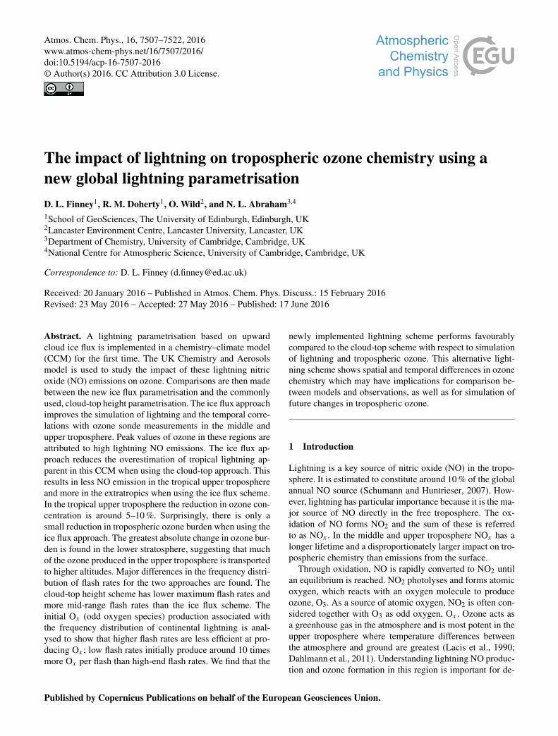
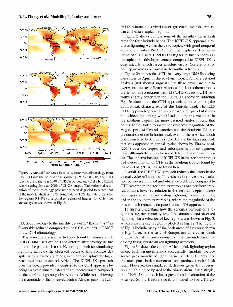
Figure 1. Annual flash rates from (a) a combined climatology fromLIS/OTD satellite observations spanning 1995–2011, (b) the CTHscheme using the year 2000 of UKCA output, and (c) the ICEFLUXscheme using the year 2000 of UKCA output. The horizontal reso-lution of the climatology product has been degraded to match thatof the model, which is 1.875◦ longitude by 1.25◦ latitude. Boxes forthe regions R1–R6 correspond to regions of interest for which theannual cycles are shown in Fig. 3.

FLUX climatology to the satellite data of 3.7 fl. km−2 yr−1 isfavourably reduced compared to the 6.0 fl. km−2 yr−1 RMSEof the CTH climatology.

These results are similar to those found by Finney et al.(2014), who used offline ERA-Interim meteorology as theinput to the parametrisation. Neither approach for simulatinglightning achieves the observed ocean to land contrast de-spite using separate equations, and neither displays the largepeak flash rate in central Africa. The ICEFLUX approachover the ocean provides a contrast to the CTH approach bybeing an overestimate instead of an underestimate comparedto the satellite lightning observations. While not achievingthe magnitude of the observed central African peak the ICE-

FLUX scheme does yield closer agreement over the Ameri-can and Asian tropical regions.

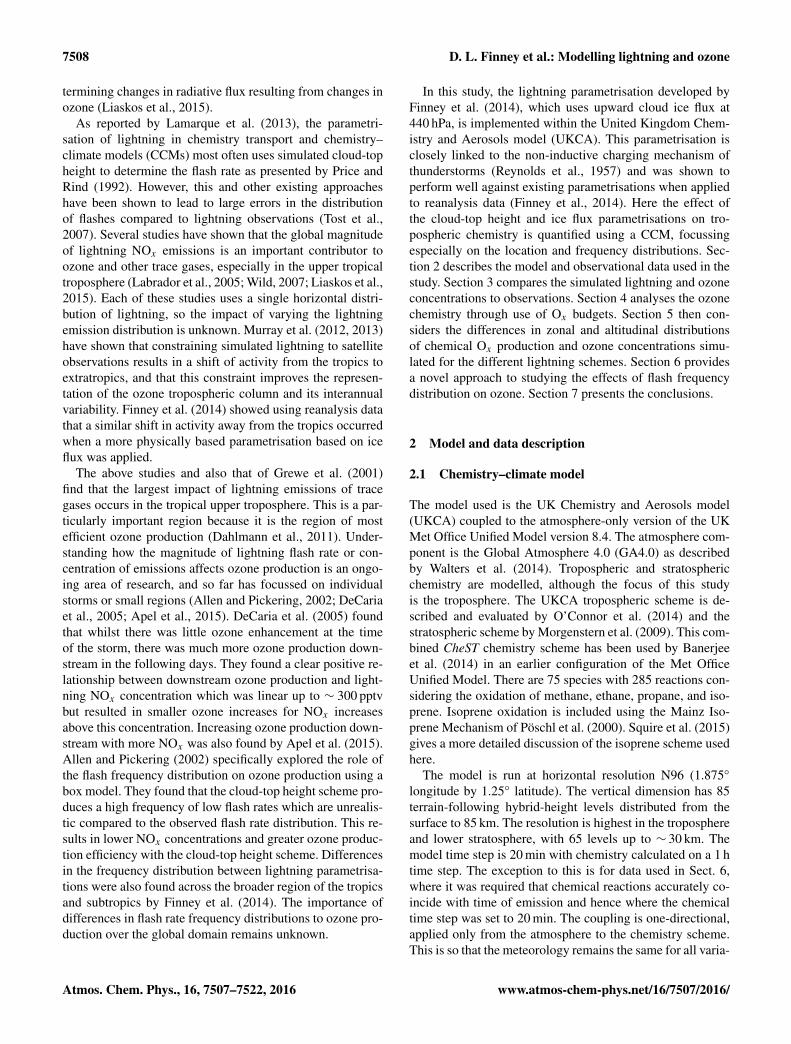
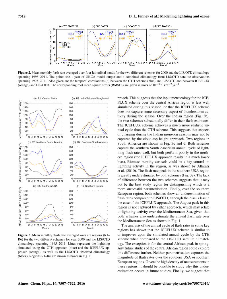
Figure 2 shows comparisons of the monthly mean flashrates for four latitude bands. The ICEFLUX approach sim-ulates lightning well in the extratropics, with good temporalcorrelations with LIS/OTD in both hemispheres. The corre-lation of CTH with LIS/OTD is higher in the southern ex-tratropics, but this improvement compared to ICEFLUX iscontrasted by much larger absolute errors. Correlations forboth approaches are lowest in the southern tropics.

Figure 2b shows that CTH has very large RMSEs duringDecember to April in the southern tropics. A more detailedanalysis (not shown) suggests that these errors are due tooverestimation over South America. In the northern tropicsthe temporal correlation with LIS/OTD suggests CTH per-forms slightly better than the ICEFLUX approach, althoughFig. 2c shows that the CTH approach is not capturing thedouble-peak characteristic of this latitude band. The ICE-FLUX approach appears to simulate a double peak but it doesnot achieve the timing, which leads to a poor correlation. Inthe northern tropics, the more detailed analysis found thatboth schemes failed to match the observed magnitude of theAugust peak of Central America and the Southern US, northe duration of the lightning peak over northern Africa whichlasts from June to September. The delay in the lightning peakthat was apparent in annual cycles shown by Finney et al.(2014) over the tropics and subtropics is not so apparenthere, although there may be some delay in the southern trop-ics. The underestimation of ICEFLUX in the northern tropicsand overestimation of CTH in the southern tropics found byFinney et al. (2014) is also found here.

Overall, the ICEFLUX approach reduces the errors in theannual cycles of lightning. This scheme improves the correla-tion between simulated and observed lightning compared toCTH scheme in the northern extratropics and southern trop-ics. It has a lower correlation in the northern tropics, whereboth approaches for simulating lightning have difficulties,and in the southern extratropics, where the magnitude of thebias is much reduced compared to the CTH approach.

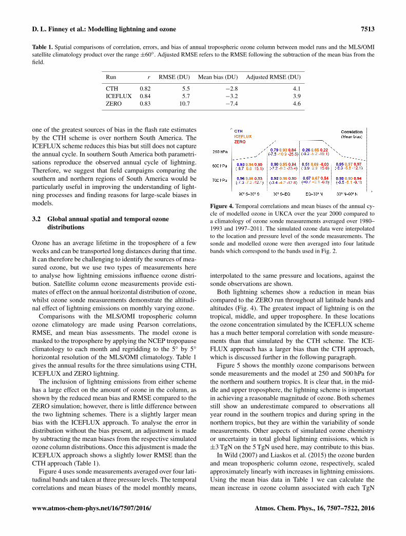
To further understand how the schemes perform on a re-gional scale, the annual cycles of the simulated and observedlightning, for a selection of key regions, are shown in Fig. 3.A box showing each region is plotted in Fig. 1a. The regionsof Fig. 3 include many of the peak areas of lightning shownin Fig. 1a or, in the case of Europe, are an area in whicha higher density of measurement studies are undertaken in-cluding using ground-based lightning detectors.

Figure 3a shows the central African peak lightning regionwhere both parametrisations successfully simulate the ob-served peak months of lightning in the LIS/OTD data. Forthe most part, both parametrisations produce similar flashrates. However, the simulated flash rates generally underes-timate lightning compared to the observations. Interestingly,the ICEFLUX approach has a greater underestimation of theobserved Spring lightning peak compared to the CTH ap-



Figure 2. Mean monthly flash rate averaged over four latitudinal bands for the two different schemes for 2000 and the LIS/OTD climatologyspanning 1995–2011. The points use 1 year of UKCA model output and a combined climatology from LIS/OTD satellite observationsspanning 1995–2011. Also given are the temporal correlations (r) between the CTH scheme (blue) and LIS/OTD and between ICEFLUX(orange) and LIS/OTD. The corresponding root mean square errors (RMSEs) are given in units of 10−3 fl. km−2 yr−1.

(a) R1: Central Africa

D J F M A M J J A S O N0

20

40

60

80

100

120

140

160

020406080100120140160

Mea

n fla

sh r

ate

(x10

-3 fl

. km

-2 d

ay-1) (b) R2: India/Pakistan/Bangladesh


20

40

60

80

100

120

140

160

(c) R3: Northern South America


20

40

60

80

100

120

140

160

020406080100120140160

Mea

n fla

sh r

ate

(x10

-3 fl

. km

-2 d

ay-1) (d) R4: Southern South America


20

40

60

80

100

120

140

160

(e) R5: Southern USA

D J F M A M J J A S O NMonth

0

20

40

60

80

100

120

140

160

020406080100120140160

Mea

n fla

sh r

ate

(x10

-3 fl

. km

-2 d

ay-1) (f) R6: Southern Europe

D J F M A M J J A S O NMonth

0

20

40

60

80

100

120

140

160

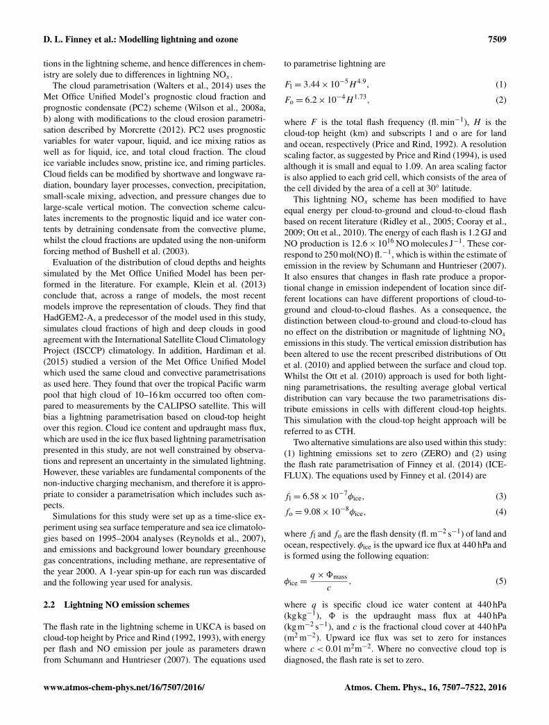
Figure 3. Mean monthly flash rate averaged over six regions (R1–R6) for the two different schemes for year 2000 and the LIS/OTDclimatology spanning 1995–2011. Lines represent the lightningsimulated using the CTH approach (blue) and the ICEFLUX ap-proach (orange), as well as the LIS/OTD observed climatology(black). Regions R1–R6 are shown as boxes in Fig. 1.

proach. This suggests that the input meteorology for the ICE-FLUX scheme over the central African region is less wellsimulated during this season, or that the ICEFLUX schemedoes not capture some necessary aspect of thunderstorm ac-tivity during the season. Over the Indian region (Fig. 3b),the two schemes substantially differ in their flash estimates.The ICEFLUX scheme achieves a much more realistic an-nual cycle than the CTH scheme. This suggests that aspectsof charging during the Indian monsoon seasons may not becaptured by the cloud-top height approach. Two regions inSouth America are shown in Fig. 3c and d. Both schemescapture the southern South American annual cycle of light-ning flash rates well, but both perform poorly in the north-ern region (the ICEFLUX approach results in a much lowerbias). Biomass burning aerosols could be a key control onlightning activity in the region, as was shown by Altaratzet al. (2010). The flash rate peak in the southern USA regionis greatly underestimated by both schemes (Fig. 3e). The lackof difference between the two schemes suggests that it maynot be the best study region for distinguishing which is amore successful parametrisation. Finally, over the southernEuropean region, both schemes show an underestimation offlash rates compared to LIS/OTD, although the bias is less inthe case of the ICEFLUX approach. The August peak in thisregion is not captured by either approach, which may relateto lightning activity over the Mediterranean Sea, given thatboth schemes also underestimate the annual flash rate overthe Mediterranean Sea as shown in Fig. 1.

The analysis of the annual cycle of flash rates in some keyregions has shown that the ICEFLUX scheme is similar toor improves upon the simulated annual cycle by the CTHscheme when compared to the LIS/OTD satellite climatol-ogy. The exception is for the central African peak in spring.Any future studies of the central African region could explorethis difference further. Neither parametrisation captures themagnitude of flash rates over the southern USA or southernEuropean regions. Given the high density of measurements inthese regions, it should be possible to study why this under-estimation occurs in future studies. Finally, we suggest that



Table 1. Spatial comparisons of correlation, errors, and bias of annual tropospheric ozone column between model runs and the MLS/OMIsatellite climatology product over the range ±60◦. Adjusted RMSE refers to the RMSE following the subtraction of the mean bias from thefield.

Run r RMSE (DU) Mean bias (DU) Adjusted RMSE (DU)

CTH 0.82 5.5 −2.8 4.1ICEFLUX 0.84 5.7 −3.2 3.9ZERO 0.83 10.7 −7.4 4.6

one of the greatest sources of bias in the flash rate estimatesby the CTH scheme is over northern South America. TheICEFLUX scheme reduces this bias but still does not capturethe annual cycle. In southern South America both parametri-sations reproduce the observed annual cycle of lightning.Therefore, we suggest that field campaigns comparing thesouthern and northern regions of South America would beparticularly useful in improving the understanding of light-ning processes and finding reasons for large-scale biases inmodels.

3.2 Global annual spatial and temporal ozonedistributions

Ozone has an average lifetime in the troposphere of a fewweeks and can be transported long distances during that time.It can therefore be challenging to identify the sources of mea-sured ozone, but we use two types of measurements hereto analyse how lightning emissions influence ozone distri-bution. Satellite column ozone measurements provide esti-mates of effect on the annual horizontal distribution of ozone,whilst ozone sonde measurements demonstrate the altitudi-nal effect of lightning emissions on monthly varying ozone.

Comparisons with the MLS/OMI tropospheric columnozone climatology are made using Pearson correlations,RMSE, and mean bias assessments. The model ozone ismasked to the troposphere by applying the NCEP tropopauseclimatology to each month and regridding to the 5◦ by 5◦

horizontal resolution of the MLS/OMI climatology. Table 1gives the annual results for the three simulations using CTH,ICEFLUX and ZERO lightning.

The inclusion of lightning emissions from either schemehas a large effect on the amount of ozone in the column, asshown by the reduced mean bias and RMSE compared to theZERO simulation; however, there is little difference betweenthe two lightning schemes. There is a slightly larger meanbias with the ICEFLUX approach. To analyse the error indistribution without the bias present, an adjustment is madeby subtracting the mean biases from the respective simulatedozone column distributions. Once this adjustment is made theICEFLUX approach shows a slightly lower RMSE than theCTH approach (Table 1).

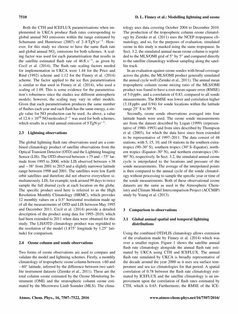
Figure 4 uses sonde measurements averaged over four lati-tudinal bands and taken at three pressure levels. The temporalcorrelations and mean biases of the model monthly means,

Figure 4. Temporal correlations and mean biases of the annual cy-cle of modelled ozone in UKCA over the year 2000 compared toa climatology of ozone sonde measurements averaged over 1980–1993 and 1997–2011. The simulated ozone data were interpolatedto the location and pressure level of the sonde measurements. Thesonde and modelled ozone were then averaged into four latitudebands which correspond to the bands used in Fig. 2.

interpolated to the same pressure and locations, against thesonde observations are shown.

Both lightning schemes show a reduction in mean biascompared to the ZERO run throughout all latitude bands andaltitudes (Fig. 4). The greatest impact of lightning is on thetropical, middle, and upper troposphere. In these locationsthe ozone concentration simulated by the ICEFLUX schemehas a much better temporal correlation with sonde measure-ments than that simulated by the CTH scheme. The ICE-FLUX approach has a larger bias than the CTH approach,which is discussed further in the following paragraph.

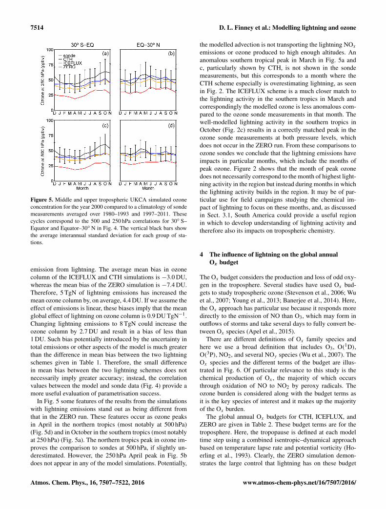
Figure 5 shows the monthly ozone comparisons betweensonde measurements and the model at 250 and 500 hPa forthe northern and southern tropics. It is clear that, in the mid-dle and upper troposphere, the lightning scheme is importantin achieving a reasonable magnitude of ozone. Both schemesstill show an underestimate compared to observations allyear round in the southern tropics and during spring in thenorthern tropics, but they are within the variability of sondemeasurements. Other aspects of simulated ozone chemistryor uncertainty in total global lightning emissions, which is±3 TgN on the 5 TgN used here, may contribute to this bias.

In Wild (2007) and Liaskos et al. (2015) the ozone burdenand mean tropospheric column ozone, respectively, scaledapproximately linearly with increases in lightning emissions.Using the mean bias data in Table 1 we can calculate themean increase in ozone column associated with each TgN



Figure 5. Middle and upper tropospheric UKCA simulated ozoneconcentration for the year 2000 compared to a climatology of sondemeasurements averaged over 1980–1993 and 1997–2011. Thesecycles correspond to the 500 and 250 hPa correlations for 30◦ S–Equator and Equator–30◦ N in Fig. 4. The vertical black bars showthe average interannual standard deviation for each group of sta-tions.

emission from lightning. The average mean bias in ozonecolumn of the ICEFLUX and CTH simulations is −3.0 DU,whereas the mean bias of the ZERO simulation is −7.4 DU.Therefore, 5 TgN of lightning emissions has increased themean ozone column by, on average, 4.4 DU. If we assume theeffect of emissions is linear, these biases imply that the meanglobal effect of lightning on ozone column is 0.9 DU TgN−1.Changing lightning emissions to 8 TgN could increase theozone column by 2.7 DU and result in a bias of less than1 DU. Such bias potentially introduced by the uncertainty intotal emissions or other aspects of the model is much greaterthan the difference in mean bias between the two lightningschemes given in Table 1. Therefore, the small differencein mean bias between the two lightning schemes does notnecessarily imply greater accuracy; instead, the correlationvalues between the model and sonde data (Fig. 4) provide amore useful evaluation of parametrisation success.

In Fig. 5 some features of the results from the simulationswith lightning emissions stand out as being different fromthat in the ZERO run. These features occur as ozone peaksin April in the northern tropics (most notably at 500 hPa)(Fig. 5d) and in October in the southern tropics (most notablyat 250 hPa) (Fig. 5a). The northern tropics peak in ozone im-proves the comparison to sondes at 500 hPa, if slightly un-derestimated. However, the 250 hPa April peak in Fig. 5bdoes not appear in any of the model simulations. Potentially,

the modelled advection is not transporting the lightning NOxemissions or ozone produced to high enough altitudes. Ananomalous southern tropical peak in March in Fig. 5a andc, particularly shown by CTH, is not shown in the sondemeasurements, but this corresponds to a month where theCTH scheme especially is overestimating lightning, as seenin Fig. 2. The ICEFLUX scheme is a much closer match tothe lightning activity in the southern tropics in March andcorrespondingly the modelled ozone is less anomalous com-pared to the ozone sonde measurements in that month. Thewell-modelled lightning activity in the southern tropics inOctober (Fig. 2c) results in a correctly matched peak in theozone sonde measurements at both pressure levels, whichdoes not occur in the ZERO run. From these comparisons toozone sondes we conclude that the lightning emissions haveimpacts in particular months, which include the months ofpeak ozone. Figure 2 shows that the month of peak ozonedoes not necessarily correspond to the month of highest light-ning activity in the region but instead during months in whichthe lightning activity builds in the region. It may be of par-ticular use for field campaigns studying the chemical im-pact of lightning to focus on these months, and, as discussedin Sect. 3.1, South America could provide a useful regionin which to develop understanding of lightning activity andtherefore also its impacts on tropospheric chemistry.

4 The influence of lightning on the global annualOx budget

The Ox budget considers the production and loss of odd oxy-gen in the troposphere. Several studies have used Ox bud-gets to study tropospheric ozone (Stevenson et al., 2006; Wuet al., 2007; Young et al., 2013; Banerjee et al., 2014). Here,the Ox approach has particular use because it responds moredirectly to the emission of NO than O3, which may form inoutflows of storms and take several days to fully convert be-tween Ox species (Apel et al., 2015).

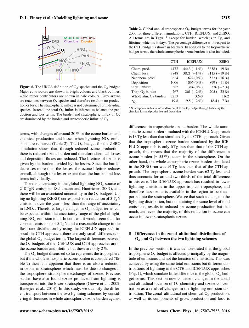
There are different definitions of Ox family species andhere we use a broad definition that includes O3, O(1D),O(3P), NO2, and several NOy species (Wu et al., 2007). TheOx species and the different terms of the budget are illus-trated in Fig. 6. Of particular relevance to this study is thechemical production of Ox , the majority of which occursthrough oxidation of NO to NO2 by peroxy radicals. Theozone burden is considered along with the budget terms asit is the key species of interest and it makes up the majorityof the Ox burden.

The global annual Ox budgets for CTH, ICEFLUX, andZERO are given in Table 2. These budget terms are for thetroposphere. Here, the tropopause is defined at each modeltime step using a combined isentropic–dynamical approachbased on temperature lapse rate and potential vorticity (Ho-erling et al., 1993). Clearly, the ZERO simulation demon-strates the large control that lightning has on these budget



Figure 6. The UKCA definition of Ox species and the Ox budget.Major contributors are shown in bright colours and black outlines,while minor contributors are shown in pale colours. Grey arrowsare reactions between Ox species and therefore result in no produc-tion or loss. The stratospheric influx is not determined for individualspecies. Instead, the total Ox influx is inferred to balance the pro-duction and loss terms. The burden and stratospheric influx of Oxare dominated by the burden and stratospheric influx of O3.

terms, with changes of around 20 % in the ozone burden andchemical production and losses when lightning NOx emis-sions are removed (Table 2). The Ox budget for the ZEROsimulation shows that, through reduced ozone production,there is reduced ozone burden and therefore chemical lossesand deposition fluxes are reduced. The lifetime of ozone isgiven by the burden divided by the losses. Since the burdendecreases more than the losses, the ozone lifetime reducesoverall, although to a lesser extent than the burden and lossterms individually.

There is uncertainty in the global lightning NOx source of2–8 TgN emissions (Schumann and Huntrieser, 2007), andthere will be an associated uncertainty in the Ox budgets. Us-ing no lightning (ZERO) corresponds to a reduction of 5 TgNemissions over the year – less than the range of uncertaintyin LNOx . Therefore, large changes in Ox budget terms canbe expected within the uncertainty range of the global light-ning NOx emission total. In contrast, it would seem that, forconstant emissions of 5 TgN and a reasonable change in theflash rate distribution by using the ICEFLUX approach in-stead the CTH approach, there are only small differences inthe global Ox budget terms. The largest differences betweenthe Ox budgets of the ICEFLUX and CTH approaches are inthe ozone burden and lifetime but these are only 2 %.

The Ox budget discussed so far represents the troposphere,but if the whole atmospheric ozone burden is considered (Ta-ble 2) then it is apparent that there is an also a reductionin ozone in stratosphere which must be due to changes inthe troposphere–stratosphere exchange of ozone. Previousstudies have also found ozone produced from lightning istransported into the lower stratosphere (Grewe et al., 2002;Banerjee et al., 2014). In this study, we quantify the differ-ent transport between the two lightning schemes by consid-ering differences in whole atmospheric ozone burden against

Table 2. Global annual tropospheric Ox budget terms for the year2000 for three different simulations: CTH, ICEFLUX, and ZERO.All terms are in Tg yr−1 except for burden, which is in Tg, andlifetime, which is in days. The percentage difference with respect tothe CTH budget is shown in brackets. In addition to the troposphericbudget terms, the whole atmospheric ozone burden is also included.

CTH ICEFLUX ZERO

Chem. prod. 4472 4443 (−1 %) 3638 (−19 %)Chem. loss 3848 3821 (−1 %) 3115 (−19 %)Net chem. prod. 624 622 (0 %) 522 (−16 %)Deposition 1006 1006 (0 %) 899 (−11 %)Strat. influx∗ 382 384 (0 %) 376 (−2 %)Trop. O3 burden 267 261 (−2 %) 205 (−23 %)Whole atm. O3 burden 3253 3240 3162τO3 19.8 19.5 (−2 %) 18.4 (−7 %)

∗ Stratospheric influx is inferred to complete the Ox budget through balancing thechemical loss and production and deposition.

differences in tropospheric ozone burden. The whole atmo-spheric ozone burden simulated with the ICEFLUX approachis 13 Tg less than that simulated by the CTH approach. Giventhat the tropospheric ozone burden simulated by the ICE-FLUX approach is only 6 Tg less than that of the CTH ap-proach, this means that the majority of the difference inozone burden (∼ 55 %) occurs in the stratosphere. On theother hand, the whole atmospheric ozone burden simulatedin the ZERO run was 91 Tg less than that of the CTH ap-proach. The tropospheric ozone burden was 62 Tg less andthus accounts for around two-thirds of the total differencein this case. The ICEFLUX approach has resulted in fewerlightning emissions in the upper tropical troposphere, andtherefore less ozone is available in the region to be trans-ported into the stratosphere. We see that such a change in thelightning distribution, but maintaining the same level of totalemissions, results in reduced net ozone production but thatmuch, and even the majority, of this reduction in ozone canoccur in lower stratospheric ozone.

5 Differences in the zonal–altitudinal distributions ofOx and O3 between the two lightning schemes

In the previous section, it was demonstrated that the globaltropospheric Ox budget is affected principally by the magni-tude of emissions and not the location of emissions. This wasachieved by using the same total emissions but different dis-tributions of lightning in the CTH and ICEFLUX approaches(Fig. 1), which simulate little difference in the global Ox bud-get terms. This section now considers changes in the zonaland altitudinal location of Ox chemistry and ozone concen-tration as a result of changes in the lightning emission dis-tribution. The zonal–altitudinal net chemical Ox production,as well as its components of gross production and loss, is



Figure 7. Annual total zonal–altitudinal distributions of Ox reaction fluxes for CTH for the year 2000. These fluxes are (a) net production,(b) gross production, and (c) gross loss of Ox . The respective differences between simulations using the ICEFLUX scheme and the CTHscheme are shown in (d–f). All units are Tg(O3). Values are annual and meridional totals. The solid line is the annual mean tropopause anddashed lines contour 10 and 100 % changes. The Ox fluxes were masked with the model tropopause every time step.

shown in Fig. 7a–c for the CTH scheme as well as changesas a result of using ICEFLUX instead of CTH in Fig. 7d–f.

The difference in net Ox production when using the ICE-FLUX scheme compared to the CTH scheme is dominatedby the change in gross production (Fig. 7d and e). Figure 7eshows a shift away from the tropical upper troposphere tothe middle troposphere and the subtropics. There is over a10 % reduction in the upper troposphere net production and100 % changes in the subtropics (Fig. 7d). However, the highsubtropical percentage change is principally due to small netproduction in these regions. The changes in Ox productionresult as a shift in emissions which happens by (1) reducedand more realistic lightning in the tropics (see Fig. 8) and(2) decoupling of the vertical and horizontal emissions distri-butions by not using cloud top in both aspects (as is the casein CTH). As described in Sect. 2.2, the column LNOx is dis-tributed up to the cloud-top, and this is how a coupling existsbetween the horizontal LNOx distribution simulated by theCTH approach and the height that LNOx emissions reach.This means that, by basing the horizontal lightning distri-bution on cloud-top height and then distributing emissionsto cloud top, LNOx is most effectively distributed to higheraltitudes. Hence, a lightning parametrisation for which thehorizontal distribution is different to that of cloud-top heightwill, to some extent, naturally distribute emissions at loweraltitudes. This is demonstrated best in Fig. 7e, which showsgross production in the northern tropics. Whilst both light-ning schemes have similar total lightning at these latitudes(shown in Fig. 8), and therefore similar column Ox produc-

Figure 8. Zonal mean lightning flash rate from the LIS/OTD clima-tology and as modelled by CTH and ICEFLUX. The zonal changesin net tropospheric column Ox production (ICEFLUX-CTH) areshown by the colour bar. The units of Ox are expressed as a mass ofozone.

tion, the gross Ox production occurs less in the upper tropo-sphere and more in the middle troposphere when using theICEFLUX scheme.

Results with the ICEFLUX approach are consistent withobservations of the zonal distribution of lightning, i.e. thatthere is less lightning in the tropics than estimated by CTHhere. Results with the ICEFLUX approach are also consis-tent with current understanding that the most intense light-



ning flash rates do not always occur in the highest clouds.We would therefore suggest that the change to the net Oxproduction of ICEFLUX is a more realistic representation ofthe distribution of production than with CTH. The improvedsonde correlations presented in Sect. 3.2 support this conclu-sion.

Whilst Ox gross production changes, mainly representingoxidation of NO to NO2 by peroxy radicals, show a close re-semblance to the lightning NO emissions changes, they areonly part of the picture with regard to changes in the distribu-tion of ozone. This is because the lifetime of ozone is muchlonger than the timescales for NO forming an equilibriumwith NO2. Furthermore, ozone precursors are transporteddownwind of convection before they form ozone. The dif-ference in Ox production (Fig. 7) between the two lightningschemes influences ozone not only locally but also down-wind, where ozone is transported to.

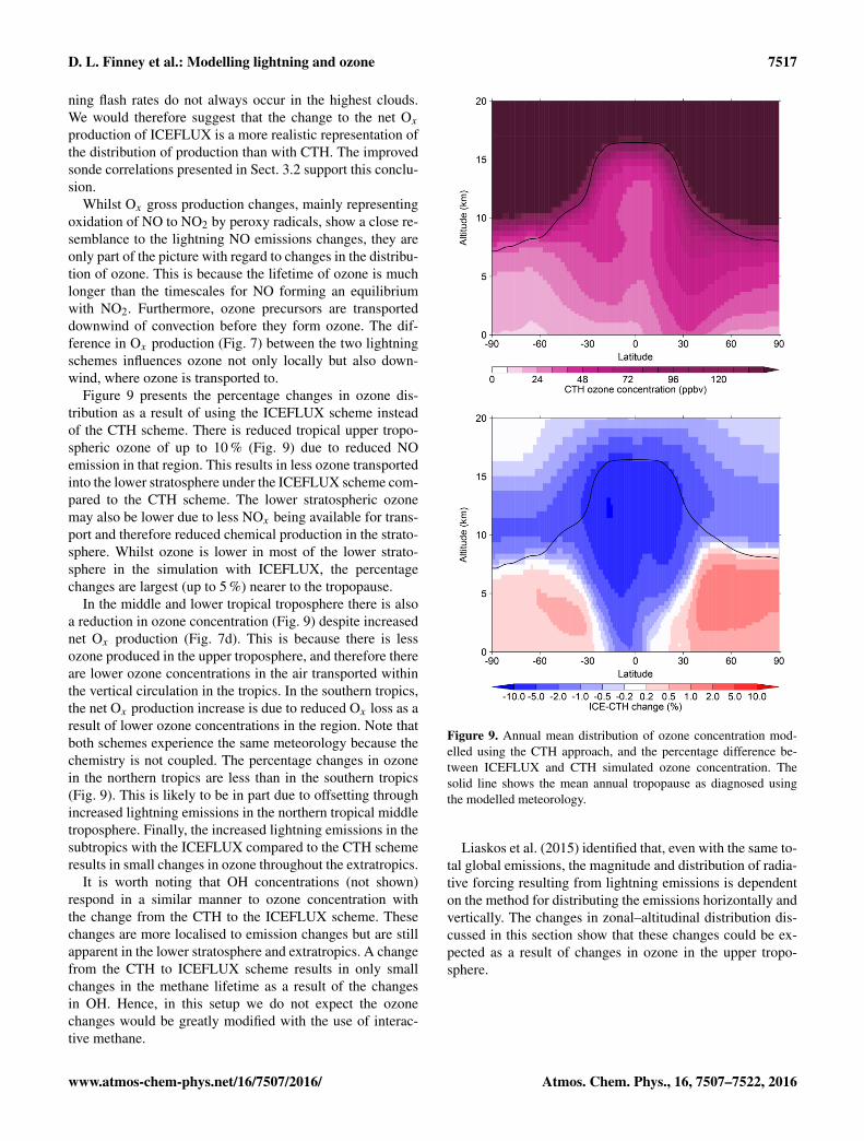
Figure 9 presents the percentage changes in ozone dis-tribution as a result of using the ICEFLUX scheme insteadof the CTH scheme. There is reduced tropical upper tropo-spheric ozone of up to 10 % (Fig. 9) due to reduced NOemission in that region. This results in less ozone transportedinto the lower stratosphere under the ICEFLUX scheme com-pared to the CTH scheme. The lower stratospheric ozonemay also be lower due to less NOx being available for trans-port and therefore reduced chemical production in the strato-sphere. Whilst ozone is lower in most of the lower strato-sphere in the simulation with ICEFLUX, the percentagechanges are largest (up to 5 %) nearer to the tropopause.

In the middle and lower tropical troposphere there is alsoa reduction in ozone concentration (Fig. 9) despite increasednet Ox production (Fig. 7d). This is because there is lessozone produced in the upper troposphere, and therefore thereare lower ozone concentrations in the air transported withinthe vertical circulation in the tropics. In the southern tropics,the net Ox production increase is due to reduced Ox loss as aresult of lower ozone concentrations in the region. Note thatboth schemes experience the same meteorology because thechemistry is not coupled. The percentage changes in ozonein the northern tropics are less than in the southern tropics(Fig. 9). This is likely to be in part due to offsetting throughincreased lightning emissions in the northern tropical middletroposphere. Finally, the increased lightning emissions in thesubtropics with the ICEFLUX compared to the CTH schemeresults in small changes in ozone throughout the extratropics.

It is worth noting that OH concentrations (not shown)respond in a similar manner to ozone concentration withthe change from the CTH to the ICEFLUX scheme. Thesechanges are more localised to emission changes but are stillapparent in the lower stratosphere and extratropics. A changefrom the CTH to ICEFLUX scheme results in only smallchanges in the methane lifetime as a result of the changesin OH. Hence, in this setup we do not expect the ozonechanges would be greatly modified with the use of interac-tive methane.

Figure 9. Annual mean distribution of ozone concentration mod-elled using the CTH approach, and the percentage difference be-tween ICEFLUX and CTH simulated ozone concentration. Thesolid line shows the mean annual tropopause as diagnosed usingthe modelled meteorology.

Liaskos et al. (2015) identified that, even with the same to-tal global emissions, the magnitude and distribution of radia-tive forcing resulting from lightning emissions is dependenton the method for distributing the emissions horizontally andvertically. The changes in zonal–altitudinal distribution dis-cussed in this section show that these changes could be ex-pected as a result of changes in ozone in the upper tropo-sphere.



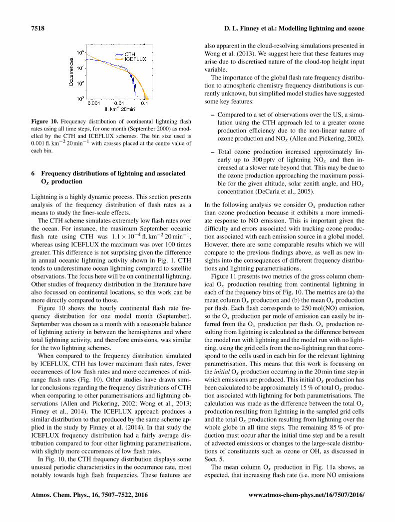
Figure 10. Frequency distribution of continental lightning flashrates using all time steps, for one month (September 2000) as mod-elled by the CTH and ICEFLUX schemes. The bin size used is0.001 fl. km−2 20min−1 with crosses placed at the centre value ofeach bin.

6 Frequency distributions of lightning and associatedOx production

Lightning is a highly dynamic process. This section presentsanalysis of the frequency distribution of flash rates as ameans to study the finer-scale effects.

The CTH scheme simulates extremely low flash rates overthe ocean. For instance, the maximum September oceanicflash rate using CTH was 1.1× 10−4 fl. km−2 20 min−1,whereas using ICEFLUX the maximum was over 100 timesgreater. This difference is not surprising given the differencein annual oceanic lightning activity shown in Fig. 1. CTHtends to underestimate ocean lightning compared to satelliteobservations. The focus here will be on continental lightning.Other studies of frequency distribution in the literature havealso focussed on continental locations, so this work can bemore directly compared to those.

Figure 10 shows the hourly continental flash rate fre-quency distribution for one model month (September).September was chosen as a month with a reasonable balanceof lightning activity in between the hemispheres and wheretotal lightning activity, and therefore emissions, was similarfor the two lightning schemes.

When compared to the frequency distribution simulatedby ICEFLUX, CTH has lower maximum flash rates, feweroccurrences of low flash rates and more occurrences of mid-range flash rates (Fig. 10). Other studies have drawn simi-lar conclusions regarding the frequency distributions of CTHwhen comparing to other parametrisations and lightning ob-servations (Allen and Pickering, 2002; Wong et al., 2013;Finney et al., 2014). The ICEFLUX approach produces asimilar distribution to that produced by the same scheme ap-plied in the study by Finney et al. (2014). In that study theICEFLUX frequency distribution had a fairly average dis-tribution compared to four other lightning parametrisations,with slightly more occurrences of low flash rates.

In Fig. 10, the CTH frequency distribution displays someunusual periodic characteristics in the occurrence rate, mostnotably towards high flash frequencies. These features are

also apparent in the cloud-resolving simulations presented inWong et al. (2013). We suggest here that these features mayarise due to discretised nature of the cloud-top height inputvariable.

The importance of the global flash rate frequency distribu-tion to atmospheric chemistry frequency distributions is cur-rently unknown, but simplified model studies have suggestedsome key features:

– Compared to a set of observations over the US, a simu-lation using the CTH approach led to a greater ozoneproduction efficiency due to the non-linear nature ofozone production and NOx (Allen and Pickering, 2002).

– Total ozone production increased approximately lin-early up to 300 pptv of lightning NOx and then in-creased at a slower rate beyond that. This may be due tothe ozone production approaching the maximum possi-ble for the given altitude, solar zenith angle, and HOxconcentration (DeCaria et al., 2005).

In the following analysis we consider Ox production ratherthan ozone production because it exhibits a more immedi-ate response to NO emission. This is important given thedifficulty and errors associated with tracking ozone produc-tion associated with each emission source in a global model.However, there are some comparable results which we willcompare to the previous findings above, as well as new in-sights into the consequences of different frequency distribu-tions and lightning parametrisations.

Figure 11 presents two metrics of the gross column chem-ical Ox production resulting from continental lightning ineach of the frequency bins of Fig. 10. The metrics are (a) themean column Ox production and (b) the mean Ox productionper flash. Each flash corresponds to 250 mol(NO) emission,so the Ox production per mole of emission can easily be in-ferred from the Ox production per flash. Ox production re-sulting from lightning is calculated as the difference betweenthe model run with lightning and the model run with no light-ning, using the grid cells from the no-lightning run that corre-spond to the cells used in each bin for the relevant lightningparametrisation. This means that this work is focussing onthe initial Ox production occurring in the 20 min time step inwhich emissions are produced. This initial Ox production hasbeen calculated to be approximately 15 % of total Ox produc-tion associated with lightning for both parametrisations. Thecalculation was made as the difference between the total Oxproduction resulting from lightning in the sampled grid cellsand the total Ox production resulting from lightning over thewhole globe in all time steps. The remaining 85 % of pro-duction must occur after the initial time step and be a resultof advected emissions or changes to the large-scale distribu-tions of constituents such as ozone or OH, as discussed inSect. 5.

The mean column Ox production in Fig. 11a shows, asexpected, that increasing flash rate (i.e. more NO emissions



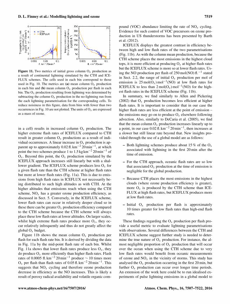
Figure 11. Two metrics of initial gross column Ox production asa result of continental lightning simulated by the CTH and ICE-FLUX schemes. The cells used in each bin correspond to thoseused in Fig. 10. The metrics are (a) mean column Ox productionin each bin and (b) mean column Ox production per flash in eachbin. The Ox production resulting from lightning was determined bysubtracting the column Ox production in the no-lightning run fromthe each lightning parametrisation for the corresponding cells. Toreduce noisiness in this figure, data from bins with fewer than twooccurrences in Fig. 10 are not plotted. The units of Ox are expressedas a mass of ozone.

in a cell) results in increased column Ox production. Thehigher extreme flash rates of ICEFLUX compared to CTHresult in greater column Ox productions as a result of indi-vidual occurrences. A linear increase in Ox production is ap-parent up to approximately 0.02 fl.km−2 20min−1, at whichpoint the two schemes produce 1 to 1.5 kgkm−2 20min−1 ofOx . Beyond this point, the Ox production simulated by theICEFLUX approach increases still linearly but with a shal-lower gradient. The ICEFLUX scheme produces less Ox fora given flash rate than the CTH scheme at higher flash ratesbut more at lower flash rates (Fig. 11a). This is due to emis-sions from high flash rates in ICEFLUX not necessarily be-ing distributed to such high altitudes as with CTH. At thehigher altitudes that emissions reach when using the CTHscheme, NOx has a greater ozone production efficiency, asdiscussed in Sect. 5. Conversely, in the ICEFLUX scheme,lower flash rates can occur in relatively deeper cloud so inthese there can be greater Ox production efficiency comparedto the CTH scheme because the CTH scheme will alwaysplace these low flash rates at lower altitudes. On larger scales,whilst high extreme flash rates produce more Ox , they oc-cur relatively infrequently and thus do not greatly affect theglobal Ox budget.

Figure 11b shows the mean column Ox production perflash for each flash rate bin. It is derived by dividing the datain Fig. 11a by the mid-point flash rate of each bin. WhilstFig. 11a shows that lower flash rates produce less Ox , theydo produce Ox more efficiently than higher flash rates. Flashrates of 0.0005 fl.km−2 20min−1 produce ∼ 10 times moreOx per flash than flash rates of 0.05 fl.km−2 20min−1. Thissuggests that NOx cycling and therefore ozone productiondecrease in efficiency as the NO increases. This is likely aresult of peroxy radical availability and volatile organic com-

pound (VOC) abundance limiting the rate of NOx cycling.Evidence for such control of VOC precursors on ozone pro-duction in US thunderstorms has been presented by Barthet al. (2012).

ICEFLUX displays the greatest contrast in efficiency be-tween high and low flash rates of the two parametrisations(Fig. 11b). As with the column mean production, because theCTH scheme places the most emissions in the highest cloudtops, it is more efficient at producing Ox at higher flash ratesbut the ICEFLUX scheme is more so at lower flash rates. Us-ing the NO production per flash of 250 mol(NO)fl.−1 statedin Sect. 2.2, the range of initial Ox production per mol ofemission is 25 mol(Ox) mol−1(NO) at low flash rates forICEFLUX to less than 2 mol(Ox) mol−1(NO) for the high-est flash rates in the ICEFLUX scheme (Fig. 11b).

In summary, we find similarly to Allen and Pickering(2002) that Ox production becomes less efficient at higherflash rates. It is important to consider that in our case thehigher flash rates are less efficient at the point of emission –the emissions may go on to produce Ox elsewhere followingadvection. Also, similarly to DeCaria et al. (2005), we findthat the mean column Ox production increases linearly up toa point, in our case 0.02 fl.km−2 20min−1, then increases ata slower but still linear rate beyond that. New insights pro-vided through the use of a global model are as follows:

– Both lightning schemes produce about 15 % of the Oxassociated with lightning in the first 20 min after thetime of emission.

– For the CTH approach, oceanic flash rates are so lowthat associated Ox production at the time of emission isnegligible for the global production.

– Because CTH places the most emissions in the highestclouds (where ozone production efficiency is greater),more Ox is produced by the CTH scheme than ICE-FLUX at high flash rates, but ICEFLUX produces moreat low flash rates.

– Initial Ox production per flash is approximately10 times greater for low flash rates than high-end flashrates.

These findings regarding the Ox production per flash pro-vide a useful metric to evaluate lightning parametrisationswith observations. Several differences between the CTH andICEFLUX scheme suggest further study is needed to deter-mine the true nature of Ox production. For instance, the al-most negligible proportion of Ox production that will occurover the ocean when using the CTH scheme due to verylow flash rates would benefit from oceanic measurementsof ozone and NOx in the vicinity of storms. This study hasanalysed the Ox production occurring in the first 20 min, butfurther Ox production can occur over longer time periods.An extension of the work here could be to run idealised ex-periments of pulse lightning emissions in a global model to



see how the Ox and ozone production develop with time andhence assess the lag between NO emission and ozone pro-duction.

7 Conclusions

A new lightning parametrisation based on upward cloud iceflux, developed by Finney et al. (2014), has been imple-mented in a chemistry–climate model (UKCA) for the firsttime. It is a physically based parametrisation closely linkedto the non-inductive charging mechanism of thunderstorms.The horizontal distribution and annual cycle of flash rates ascalculated through the new ice flux approach and the com-monly used, cloud-top height approach were compared tothe LIS/OTD satellite climatology. The ice flux approach isshown to generally improve upon the performance of thecloud-top height approach. Of particular importance is therealistic representation of the zonal distribution of lightningusing the ice flux approach, whereas the cloud-top height ap-proach overestimates the amount of tropical lightning andunderestimates extratropical lightning.

The ice flux approach greatly improves upon the cloud-topheight approach in UKCA with regard to the temporal corre-lation to the observed annual cycle of ozone in the middleand upper tropical troposphere. Through considering a sim-ulation without emissions and the simulated annual cycle oflightning, it is clear that the ice flux approach reduces the bi-ases in ozone in months where the cloud-top height approachhas the largest errors in simulating lightning.

The zonal flash rate distribution when using the ice fluxapproach instead of the cloud-top height approach results ina shift of Ox production away from the upper tropical tro-posphere. As a consequence there is a 5–10 % reduction inupper tropical tropospheric ozone concentration along withsmaller reductions in the lower stratosphere and small in-creases in the extratropical troposphere. These changes inozone concentration are a result of the change in distribu-tion of lightning emissions only; the total global emissionsare the same for both schemes. We conclude that biases inzonal lightning distribution of the cloud-top height schemeincrease ozone in the upper tropical troposphere and, asdemonstrated by comparison to ozone sondes, this reducesthe correlation to observations in ozone annual cycle in thisregion.

Analysis of the continental flash rate frequency distribu-tion shows the cloud-top height approach has lower high-endextreme flash rates, more frequent mid-range flash rates, andless frequent low-end flash rates compared to the frequencydistribution using the ice flux approach. Such features sim-ulated by the cloud-top height approach have been found incomparisons to the observed frequency distribution over theUS, and this current evidence suggests such a frequency dis-tribution is unrealistic. We apply a novel analysis to deter-mine the impact of the differences in flash rate frequency dis-

tribution on the initial Ox production resulting from lightningemissions. As expected, the higher the flash rate, the more Oxis initially produced. However, the Ox production efficiencyreduces for higher flash rates; lower flash rates initially pro-duce approximately 10 times as much Ox as higher flashrates. Further study is warranted to determine how emissionsproduce ozone downstream of a storm in complex chem-istry models, but the result here is relevant to aircraft cam-paigns measuring NOx and ozone near to the thunderstorms.It would be useful to study such measurements to determinewhether less intense storms exhibit such a difference in Oxproduction efficiency.

The global lightning parametrisation of Finney et al.(2014) using upward cloud ice flux has proven to be ro-bust at simulating present-day annual distributions of light-ning and tropospheric ozone. The reduced ozone in the uppertropical troposphere could be important for the understand-ing of ozone radiative forcing. In addition, the differencesin the frequency distribution when using different lightningschemes are shown to affect the chemical Ox production.The parametrisation is appropriate for testing in other chem-istry transport and chemistry–climate models, where it willbe important to determine how the parametrisation behavesusing different convective schemes. Furthermore, this newparametrisation offers an opportunity to diversify the esti-mates of the sensitivity of lightning to climate change, whichwill be the focus of future work.

Author contributions. D. L. Finney, R. M. Doherty, O. Wild, andN. L. Abraham designed the experiments and interpreted the results.D. L. Finney performed the analysis. D. L. Finney and N. L. Abra-ham developed the code and ran simulations. D. L. Finney preparedthe manuscript with contributions from all co-authors.

Acknowledgements. This work has been supported by a NaturalEnvironment Research Council grant (NE/K500835/1). We thankthe TRMM satellite team for access to the Lightning ImagingSensor products. Thanks to Paul Young for providing and assist-ing with use of the ozone column and sonde observations, andJonathan Wilkinson for guidance regarding implementation ofthe lightning parametrisation based on ice flux in the Met OfficeUnified Model. Finally, we thank the two anonymous reviewers,who greatly helped to improve the manuscript.

Edited by: P. Jöckel

References

Allen, D. J. and Pickering, K. E.: Evaluation of lightning flash rateparameterizations for use in a global chemical transport model,J. Geophys. Res., 107, 4711, doi:10.1029/2002JD002066, 2002.

Altaratz, O., Koren, I., Yair, Y., and Price, C.: Lightning responseto smoke from Amazonian fires, Geophys. Res. Lett., 37, 1–6,doi:10.1029/2010GL042679, 2010.


http://dx.doi.org/10.1029/2002JD002066

http://dx.doi.org/10.1029/2010GL042679


Apel, E. C., Hornbrook, R. S., Hills, A. J., Blake, N. J., Barth,M. C., Weinheimer, A., Cantrell, C., Rutledge, S. A., Basarab, B.,Crawford, J., Diskin, G., Homeyer, C. R., Campos, T., Flocke,F., Fried, A., Blake, D. R., Brune, W., Pollack, I., Peischl,J., Ryerson, T., Wennberg, P. O., Crounse, J. D., Wisthaler,A., Mikoviny, T., Huey, G., Heikes, B., Sullivan, D. O., andRiemer, D. D.: Upper tropospheric ozone production from light-ning NOx -impacted convection: Smoke ingestion case studyfrom the DC3 campaign, J. Geophys. Res. Atmos., 120, 1–19,doi:10.1002/2014JD022121, 2015.

Banerjee, A., Archibald, A. T., Maycock, A. C., Telford, P., Abra-ham, N. L., Yang, X., Braesicke, P., and Pyle, J. A.: LightningNOx , a key chemistry–climate interaction: impacts of future cli-mate change and consequences for tropospheric oxidising capac-ity, Atmos. Chem. Phys., 14, 9871–9881, doi:10.5194/acp-14-9871-2014, 2014.

Barth, M. C., Lee, J., Hodzic, A., Pfister, G., Skamarock, W. C.,Worden, J., Wong, J., and Noone, D.: Thunderstorms and uppertroposphere chemistry during the early stages of the 2006 NorthAmerican Monsoon, Atmos. Chem. Phys., 12, 11003–11026,doi:10.5194/acp-12-11003-2012, 2012.

Bushell, A. C., Wilson, D. R., and Gregory, D.: A descriptionof cloud production by non-uniformly distributed processes, Q.J. Roy. Meteor. Soc., 129, 1435–1455, doi:10.1256/qj.01.110,2003.

Cecil, D. J., Buechler, D. E., and Blakeslee, R. J.: Grid-ded lightning climatology from TRMM-LIS and OTD:Dataset description, Atmos. Res., 135-136, 404–414,doi:10.1016/j.atmosres.2012.06.028, 2014.

Cooray, V., Rahman, M., and Rakov, V.: On the NOx produc-tion by laboratory electrical discharges and lightning, J. Atmos.Sol.-Terr. Phy., 71, 1877–1889, doi:10.1016/j.jastp.2009.07.009,2009.

Dahlmann, K., Grewe, V., Ponater, M., and Matthes, S.: Quanti-fying the contributions of individual NOx sources to the trendin ozone radiative forcing, Atmos. Environ., 45, 2860–2868,doi:10.1016/j.atmosenv.2011.02.071, 2011.

DeCaria, A. J., Pickering, K. E., Stenchikov, G. L., and Ott,L. E.: Lightning-generated NOx and its impact on tropo-spheric ozone production: A three-dimensional modeling studyof a Stratosphere-Troposphere Experiment: Radiation, Aerosolsand Ozone (STERAO-A) thunderstorm, J. Geophys. Res., 110,D14303, doi:10.1029/2004JD005556, 2005.

Finney, D. L., Doherty, R. M., Wild, O., Huntrieser, H., Pumphrey,H. C., and Blyth, A. M.: Using cloud ice flux to parametriselarge-scale lightning, Atmos. Chem. Phys., 14, 12665–12682,doi:10.5194/acp-14-12665-2014, 2014.

Grewe, V., Brunner, D., Dameris, M., Grenfell, J., Hein, R.,Shindell, D., and Staehelin, J.: Origin and variability of up-per tropospheric nitrogen oxides and ozone at northern mid-latitudes, Atmos. Environ., 35, 3421–3433, doi:10.1016/S1352-2310(01)00134-0, 2001.

Grewe, V., Reithmeier, C., and Shindell, D. T.: Dynamic-chemicalcoupling of the upper troposphere and lower stratosphere region,Chemosphere, 47, 851–61, 2002.

Hardiman, S. C., Boutle, I. A., Bushell, A. C., Butchart, N., Cullen,M. J. P., Field, P. R., Furtado, K., Manners, J. C., Milton, S. F.,Morcrette, C., O’Connor, F. M., Shipway, B. J., Smith, C., Wal-ters, D. N., Willett, M. R., Williams, K. D., Wood, N., Lukeabra-

ham, N., Keeble, J., Maycock, A. C., Thuburn, J., and Wood-house, M. T.: Processes controlling tropical tropopause tempera-ture and stratospheric water vapor in climate models, J. Climate,28, 6516–6535, doi:10.1175/JCLI-D-15-0075.1, 2015.

Hoerling, M. P., Schaack, T. K., and Lenzen, A. J.: A global analysisof stratospheric–tropospheric exchange during northern winter,doi:10.1175/1520-0493(1993)121<0162:AGAOSE>2.0.CO;2,1993.

Klein, S. A., Zhang, Y., Zelinka, M. D., Pincus, R., Boyle, J., andGleckler, P. J.: Are climate model simulations of clouds improv-ing? An evaluation using the ISCCP simulator, J. Geophys. Res.-Atmos., 118, 1329–1342, doi:10.1002/jgrd.50141, 2013.

Labrador, L. J., von Kuhlmann, R., and Lawrence, M. G.: Theeffects of lightning-produced NOx and its vertical distributionon atmospheric chemistry: sensitivity simulations with MATCH-MPIC, Atmos. Chem. Phys., 5, 1815–1834, doi:10.5194/acp-5-1815-2005, 2005.

Lacis, A. A., Wuebbles, D. J., and Logan, J. A.: Radiative forc-ing of climate by changes in the vertical distribution of ozone, J.Geophys. Res., 95, 9971–9981, doi:10.1029/JD095iD07p09971,1990.

Lamarque, J.-F., Shindell, D. T., Josse, B., Young, P. J., Cionni, I.,Eyring, V., Bergmann, D., Cameron-Smith, P., Collins, W. J., Do-herty, R., Dalsoren, S., Faluvegi, G., Folberth, G., Ghan, S. J.,Horowitz, L. W., Lee, Y. H., MacKenzie, I. A., Nagashima, T.,Naik, V., Plummer, D., Righi, M., Rumbold, S. T., Schulz, M.,Skeie, R. B., Stevenson, D. S., Strode, S., Sudo, K., Szopa, S.,Voulgarakis, A., and Zeng, G.: The Atmospheric Chemistry andClimate Model Intercomparison Project (ACCMIP): overviewand description of models, simulations and climate diagnostics,Geosci. Model Dev., 6, 179–206, doi:10.5194/gmd-6-179-2013,2013.

Liaskos, C. E., Allen, D. J., and Pickering, K. E.: Sen-sitivity of Tropical Tropospheric Composition to Light-ning NOx Production as Determined by the NASA GEOS-Replay Model, J. Geophys. Res.-Atmos., 120, 8512–8534,doi:10.1002/2014JD022987, 2015.

Logan, J. A.: An analysis of ozonesonde data for the troposphere:Recommendations for testing 3-D models and development ofa gridded climatology for tropospheric ozone, J. Geophys. Res.,104, 16115–16149, doi:10.1029/1998JD100096, 1999.

Morcrette, C. J.: Improvements to a prognostic cloud schemethrough changes to its cloud erosion parametrization, Atmos. Sci.Lett., 13, 95–102, doi:10.1002/asl.374, 2012.

Morgenstern, O., Braesicke, P., O’Connor, F. M., Bushell, A. C.,Johnson, C. E., Osprey, S. M., and Pyle, J. A.: Evaluation ofthe new UKCA climate-composition model – Part 1: The strato-sphere, Geosci. Model Dev., 2, 43–57, doi:10.5194/gmd-2-43-2009, 2009.

Murray, L. T., Jacob, D. J., Logan, J. A., Hudman, R. C., andKoshak, W. J.: Optimized regional and interannual variabilityof lightning in a global chemical transport model constrainedby LIS/OTD satellite data, J. Geophys. Res., 117, D20307,doi:10.1029/2012JD017934, 2012.

Murray, L. T., Logan, J. A., and Jacob, D. J.: Interannual variabilityin tropical tropospheric ozone and OH : the role of lightning,J. Geophys. Res., 118, 11468–11480, doi:10.1002/jgrd.50857,2013.


http://dx.doi.org/10.1002/2014JD022121

http://dx.doi.org/10.5194/acp-14-9871-2014



http://dx.doi.org/10.1256/qj.01.110

http://dx.doi.org/10.1016/j.atmosres.2012.06.028

http://dx.doi.org/10.1016/j.jastp.2009.07.009

http://dx.doi.org/10.1016/j.atmosenv.2011.02.071

http://dx.doi.org/10.1029/2004JD005556


http://dx.doi.org/10.1016/S1352-2310(01)00134-0

http://dx.doi.org/10.1016/S1352-2310(01)00134-0

http://dx.doi.org/10.1175/JCLI-D-15-0075.1

http://dx.doi.org/10.1175/1520-0493(1993)121<0162:AGAOSE>2.0.CO;2

http://dx.doi.org/10.1002/jgrd.50141



http://dx.doi.org/10.1029/JD095iD07p09971

http://dx.doi.org/10.5194/gmd-6-179-2013

http://dx.doi.org/10.1002/2014JD022987

http://dx.doi.org/10.1029/1998JD100096

http://dx.doi.org/10.1002/asl.374



http://dx.doi.org/10.1029/2012JD017934

http://dx.doi.org/10.1002/jgrd.50857


O’Connor, F. M., Johnson, C. E., Morgenstern, O., Abraham, N.L., Braesicke, P., Dalvi, M., Folberth, G. A., Sanderson, M. G.,Telford, P. J., Voulgarakis, A., Young, P. J., Zeng, G., Collins,W. J., and Pyle, J. A.: Evaluation of the new UKCA climate-composition model – Part 2: The Troposphere, Geosci. ModelDev., 7, 41–91, doi:10.5194/gmd-7-41-2014, 2014.

Ott, L. E., Pickering, K. E., Stenchikov, G. L., Allen, D. J.,DeCaria, A. J., Ridley, B., Lin, R.-F., Lang, S., and Tao,W.-K.: Production of lightning NOx and its vertical distri-bution calculated from three-dimensional cloud-scale chemicaltransport model simulations, J. Geophys. Res., 115, D04301,doi:10.1029/2009JD011880, 2010.

Pöschl, U., von Kuhlmann, R., Poisson, N., and Crutzen, P. J.: De-velopment and Intercomparison of Condensed Isoprene Oxida-tion Mechanisms for Global Atmospheric Modeling, J. Atmos.Chem, 37, 29–52, doi:10.1023/A:1006391009798, 2000.

Price, C. and Rind, D.: A simple lightning parameterization forcalculating global lightning distributions, J. Geophys. Res., 97,9919–9933, doi:10.1029/92JD00719, 1992.

Price, C. and Rind, D.: What determines the cloud-to-ground light-ning fraction in thunderstorms?, Geophys. Res. Lett., 20, 463–466, doi:10.1029/93GL00226, 1993.

Price, C. and Rind, D.: Modeling global lightning distributions in ageneral circulation model, Mon. Weather Rev., 122, 1930–1939,1994.

Reynolds, R. W., Smith, T. M., Liu, C., Chelton, D. B., Casey,K. S., and Schlax, M. G.: Daily high-resolution-blended anal-yses for sea surface temperature, J. Climate, 20, 5473–5496,doi:10.1175/2007JCLI1824.1, 2007.

Reynolds, S. E., Brook, M., and Gourley, M. F.: Thunderstormcharge separation, J. Meteorol., 14, 426–436, 1957.

Ridley, B., Pickering, K., and Dye, J.: Comments on theparameterization of lightning-produced NO in globalchemistry-transport models, Atmos. Environ., 39, 6184–6187,doi:10.1016/j.atmosenv.2005.06.054, 2005.

Schumann, U. and Huntrieser, H.: The global lightning-inducednitrogen oxides source, Atmos. Chem. Phys., 7, 3823–3907,doi:10.5194/acp-7-3823-2007, 2007.

Squire, O. J., Archibald, A. T., Griffiths, P. T., Jenkin, M. E., Smith,D., and Pyle, J. A.: Influence of isoprene chemical mechanism onmodelled changes in tropospheric ozone due to climate and landuse over the 21st century, Atmos. Chem. Phys., 15, 5123–5143,doi:10.5194/acp-15-5123-2015, 2015.

Stevenson, D. S., Dentener, F. J., Schultz, M. G., Ellingsen, K.,van Noije, T. P. C., Wild, O., Zeng, G., Amann, M., Ather-ton, C. S., Bell, N., Bergmann, D. J., Bey, I., Butler, T., Co-fala, J., Collins, W. J., Derwent, R. G., Doherty, R. M., Drevet,J., Eskes, H. J., Fiore, A. M., Gauss, M., Hauglustaine, D. A.,Horowitz, L. W., Isaksen, I. S. A., Krol, M. C., Lamarque, J.-F.,Lawrence, M. G., Montanaro, V., Müller, J.-F., Pitari, G., Prather,M. J., Pyle, J. A., Rast, S., Rodriguez, J. M., Sanderson, M. G.,Savage, N. H., Shindell, D. T., Strahan, S. E., Sudo, K., andSzopa, S.: Multimodel ensemble simulations of present-day andnear-future tropospheric ozone, J. Geophys. Res., 111, D08301,doi:10.1029/2005JD006338, 2006.

Thompson, A. M., Witte, J. C., Oltmans, S. J., Schmidlin, F. J.,Logan, J. A., Fujiwara, M., Kirchhoff, V. W. J. H., Posny, F.,Coetzee, G. J. R., Hoegger, B., Kawakami, S., Ogawa, T., For-tuin, J. P. F., and Kelder, H. M.: Southern Hemisphere Additional

Ozonesondes (SHADOZ) 1998–2000 tropical ozone climatology2. Tropospheric variability and the zonal wave-one, J. Geophys.Res., 108, 8241, doi:10.1029/2002JD002241, 2003.

Tost, H., Jöckel, P., and Lelieveld, J.: Lightning and convec-tion parameterisations – uncertainties in global modelling, At-mos. Chem. Phys., 7, 4553–4568, doi:10.5194/acp-7-4553-2007,2007.

Walters, D. N., Williams, K. D., Boutle, I. A., Bushell, A. C., Ed-wards, J. M., Field, P. R., Lock, A. P., Morcrette, C. J., Strat-ton, R. A., Wilkinson, J. M., Willett, M. R., Bellouin, N., Bodas-Salcedo, A., Brooks, M. E., Copsey, D., Earnshaw, P. D., Hardi-man, S. C., Harris, C. M., Levine, R. C., MacLachlan, C., Man-ners, J. C., Martin, G. M., Milton, S. F., Palmer, M. D., Roberts,M. J., Rodríguez, J. M., Tennant, W. J., and Vidale, P. L.: TheMet Office Unified Model Global Atmosphere 4.0 and JULESGlobal Land 4.0 configurations, Geosci. Model Dev., 7, 361–386,doi:10.5194/gmd-7-361-2014, 2014.

Wild, O.: Modelling the global tropospheric ozone budget: explor-ing the variability in current models, Atmos. Chem. Phys., 7,2643–2660, doi:10.5194/acp-7-2643-2007, 2007.

Wilson, D. R., Bushell, A. C., Kerr-Munslow, A. M., Price, J. D.,and Morcrette, C. J.: PC2: A prognostic cloud fraction and con-densation scheme. I: Scheme description, Q. J. Roy. Meteor.Soc., 134, 2093–2107, doi:10.1002/qj.333, 2008a.

Wilson, D. R., Bushell, A. C., Kerr-Munslow, A. M., Price,J. D., Morcrette, C. J., and Bodas-Salcedob, A.: PC2: A prog-nostic cloud fraction and condensation scheme. II: Climatemodel simulations, Q. J. Roy. Meteor. Soc., 134, 2109–2125,doi:10.1002/qj.332, 2008b.

Wong, J., Barth, M. C., and Noone, D.: Evaluating a lightningparameterization based on cloud-top height for mesoscale nu-merical model simulations, Geosci. Model Dev., 6, 429–443,doi:10.5194/gmd-6-429-2013, 2013.

Wu, S., Mickley, L. J., Jacob, D. J., Logan, J. A., Yantosca, R. M.,and Rind, D.: Why are there large differences between modelsin global budgets of tropospheric ozone?, J. Geophys. Res., 112,D05302, doi:10.1029/2006JD007801, 2007.

Young, P. J., Archibald, A. T., Bowman, K. W., Lamarque, J.-F.,Naik, V., Stevenson, D. S., Tilmes, S., Voulgarakis, A., Wild, O.,Bergmann, D., Cameron-Smith, P., Cionni, I., Collins, W. J., Dal-søren, S. B., Doherty, R. M., Eyring, V., Faluvegi, G., Horowitz,L. W., Josse, B., Lee, Y. H., MacKenzie, I. A., Nagashima, T.,Plummer, D. A., Righi, M., Rumbold, S. T., Skeie, R. B., Shin-dell, D. T., Strode, S. A., Sudo, K., Szopa, S., and Zeng, G.: Pre-industrial to end 21st century projections of tropospheric ozonefrom the Atmospheric Chemistry and Climate Model Intercom-parison Project (ACCMIP), Atmos. Chem. Phys., 13, 2063–2090, doi:10.5194/acp-13-2063-2013, 2013.

Ziemke, J. R., Chandra, S., Labow, G. J., Bhartia, P. K., Froidevaux,L., and Witte, J. C.: A global climatology of tropospheric andstratospheric ozone derived from Aura OMI and MLS measure-ments, Atmos. Chem. Phys., 11, 9237–9251, doi:10.5194/acp-11-9237-2011, 2011.



http://dx.doi.org/10.1029/2009JD011880

http://dx.doi.org/10.1023/A:1006391009798

http://dx.doi.org/10.1029/92JD00719

http://dx.doi.org/10.1029/93GL00226

http://dx.doi.org/10.1175/2007JCLI1824.1

http://dx.doi.org/10.1016/j.atmosenv.2005.06.054



http://dx.doi.org/10.1029/2005JD006338

http://dx.doi.org/10.1029/2002JD002241




http://dx.doi.org/10.1002/qj.333

http://dx.doi.org/10.1002/qj.332


http://dx.doi.org/10.1029/2006JD007801




acp-16-7507-2016 | acp

Documents