1

ACCURACY ASSESSMENT OF LIDAR ELEVATION DATA USING SURVEY MARKS

Xiaoye Liu

1, 2

1 Centre for GIS, School of Geography and Environmental Science, Monash

University, Clayton VIC 3800, Australia 2 Australian Centre for Sustainable Catchments, and Faculty of Engineering and

Surveying, University of Southern Queensland Toowoomba QLD 4350, Australia

Email: xiaoye.liu@usq.edu.au

ABSTRACT Airborne LiDAR has become the preferred technology for digital elevation data acquisition in a wide

range of applications. The vertical accuracy with respect to a specified vertical datum is the principal

criterion in specifying the quality of LiDAR elevation data. The quantitative assessment of LiDAR

elevation data is usually conducted by comparing high-accuracy checkpoints with elevations estimated

from the LiDAR ground data. However, the collection of a sufficient number of checkpoints by field

surveying is a time-consuming task. This study used survey marks to assess the vertical accuracy of

LiDAR data for different land covers in a rural area and explored the performance of different methods

for deriving elevations from LiDAR data corresponding to the locations of checkpoints. Normality tests

using both frequency histograms and quantile-quantile plots were performed for vertical differences

between the LiDAR data and the checkpoints, so the appropriate measures (the formula 1.96×RMSE or

the 95th

percentile) can be used for the vertical accuracy assessment of the LiDAR data for different

land covers. The results demonstrated the suitability of using survey marks as checkpoints for the

assessment of the vertical accuracy of LiDAR data.

KEYWORDS: LiDAR, Airborne laser scanning, Digital elevation model, Survey mark, Accuracy assessment

INTRODUCTION

Airborne light detection and ranging (LiDAR), also referred to as airborne laser scanning (ALS), is one of the most effective means of terrain data collection. Using LiDAR data for the generation of digital elevation models (DEM) is becoming a standard practice in the spatial science community [10]. One of the appealing features in the LiDAR output is the high-density and high-accuracy of the three-dimensional coordinates of point, as characterised by the vertical accuracy of 10-50 cm RMSE (root mean square error) at 68% confidence level (or 19.6-98 cm at 95% confidence level) and the horizontal point spacing of 1-3 m [13]. A higher vertical accuracy of 10-15 cm RMSE (at 68% confidence level) can only be achieved under the most ideal circumstances [10]. The actual accuracy of LiDAR elevation data in a project depends on the flying height, laser beam divergence, location of the reflected point within the swathe, LiDAR system errors including errors from the Global Positioning System (GPS) and the Inertial Measurement Unit (IMU), the distance to the GPS ground base station, and the LiDAR data classification (filtering) reliability [10], [27]. Methods for the quality assessment of LiDAR data also vary with applications and the delivery format of the LiDAR data. For the purpose of a DEM generation, delivered with classified LiDAR point clouds, the vertical accuracy with respect to a specified vertical datum is the principal criterion in specifying the quality of the LiDAR elevation data [19]. The quantitative assessment of the LiDAR elevation data is usually conducted by comparing high-accuracy checkpoints with elevations estimated from the LiDAR

2

ground data. Checkpoints should come from independent sources and be at least three times more accurate than the dataset to be tested [21]. The accuracy of LiDAR data is also affected by the types of ground cover because the vegetation can limit ground detection. Areas with tall and dense vegetation tend to cause greater elevation errors than open terrain does [21]. Therefore, the checkpoints should be distributed over all major land cover types. ASPRS (American Society for Photogrammetry and Remote Sensing) and ICSM (Inter-Governmental Committee on Surveying and Mapping) recommend collecting a minimum of 20 checkpoints (30 is preferred) in each of the major land cover categories representative of the area for which the vertical accuracy of LiDAR data is to be verified [2], [13]. Specifying a minimum of 20 checkpoints for each of the major land cover types is necessary for a practical level of confidence in the statistical calculations. Obviously, a large number of checkpoints will provide more confidence in practice [20]. However, the collection of a large number of high-accuracy checkpoints is a time-consuming task even with GPS, leading to an increase of the costs of a project. The survey marks of the geodetic control have high-accuracy coordinates relative to the national horizontal and vertical datums. In some areas like in Victoria, Australia, there is a high density of survey marks. Existing survey marks with a higher accuracy of elevation values provide a potential for the efficient collection of checkpoints. An experiment testing the suitability of survey marks as checkpoints for the accuracy assessment of LiDAR data is needed. Once survey marks (here, used as checkpoints) are collected, the elevations from LiDAR data corresponding to each checkpoint are derived to compare with the elevations of the checkpoints. Given that the LiDAR data are used to predict the elevation value for a specific location (the location of the checkpoint), instead of the prediction of the entire terrain surface, the elevation corresponding to each checkpoint can be obtained from the LiDAR points which are around the checkpoint. The LiDAR data points within a specific radius around each checkpoint can be selected as a sub-dataset, so that the LiDAR elevations corresponding to each of the checkpoints can be derived from the sub-datasets. There are several ways to derive the corresponding elevations from these sub-set LiDAR data. For example, they can either be interpolated from the surrounding data using interpolation algorithms, obtained from constructed TIN (triangulated irregular networks) around each checkpoint or from the elevation of the nearest point [29]. Elevations from LiDAR data at the location of each checkpoint may vary with the used methods. This will affect the results of the accuracy assessment. Although some research has been done to compare the performance of some commonly used interpolators in the context of model accuracy, few studies have been conducted on the performance of the different methods used to extract the elevations from LiDAR data for the purpose of an overall absolute accuracy assessment. This study aims to assess the vertical accuracy of LiDAR data for different land cover categories in a large rural area using survey marks and explore the performance of the different methods for deriving the elevations from LiDAR data at the location of each checkpoint. The remainder of this paper is organised as follows. Airborne LiDAR is briefly introduced first. The next section describes the geodetic survey marks, their status in Victoria, Australia, and the suitability of using survey marks as checkpoints to assess the vertical accuracy of LiDAR data. This is followed by three sections describing the study area, LiDAR data and checkpoints and the methodology used for this study. The testing of the normal distribution, a vertical accuracy assessment of the LiDAR data for different land covers and the methods used for deriving the elevations from LiDAR data at the locations of the checkpoints are presented and discussed in a

3

result and a discussion section. Finally, conclusions are drawn.

AIRBORNE LIDAR

LiDAR is an active remote sensing technology [31]. It actively transmits pulses of laser light toward an object of interest, and receives the light that is scattered and reflected by the objects [32]. An airborne LiDAR system is typically composed of three components: a laser scanner unit, a GPS receiver and an IMU [8], [9], [12], [31]. The laser scanner unit consists of a pulse generator (Nd:YAG laser) with a wavelength in the range of 0.8 µm to 1.6 µm (typically, 1.064 µm or 1.500 µm) and a receiver to get the pulses scattered and reflected by the targets [22], [31]. The laser pulses are emitted at a rate of up to 250 kHz to the Earth surface [15]. The distance (range) between the LiDAR sensor and the target is calculated by multiplying the speed of light by half of the time it takes for the light to travel from the sensor to the target and back [32]. The GPS receiver is used to record the aircraft trajectory and the IMU measures the attitude of the aircraft (roll, pitch, and yaw or heading) [30]. The calculated range between the scanner and the target and the position and orientation information obtained from the GPS and IMU units are used to determine the target location in three-dimensional space [31]. The three-dimensional LiDAR points are initially represented by latitude, longitude, and ellipsoidal height based on the WGS84 reference ellipsoid. They can then be transformed to a national or regional coordinate system. During this process, elevations are converted from ellipsoidal heights to ortho-metric heights based on a national or regional height datum [18], [30]. Airborne LiDAR systems are also capable of detecting multiple return signals for a single transmitted pulse [31]. Most LiDAR systems typically record the first and last returns, but some are able to record up to six returns for a single pulse [16]. Multiple returns occur when a laser pulse strikes a target that does not completely block the path of the pulse and the remaining portion of the pulse continues on to a lower object. This situation frequently occurs in forested areas where there are some gaps between branches and foliage [24]. Recording multiple returns is useful for the topographic mapping in forested area [26]. For the purpose of a DEM generation, one of the critical steps is to separate the LiDAR points into ground (terrain) and non-ground points [17]. Some filter algorithms have been developed for automatically extracting ground points from all recorded LiDAR points [4], [14], [28], [34].

SURVEY MARKS AND SUITABILITY FOR CHECKPOINTS

Geodetic control surveys are usually performed to establish a framework of positions that provides a common reference system for establishing the coordinates of all spatial data [7]. Survey control marks are the basis of the geodetic control framework and an important component of the spatial data infrastructure. The geodetic survey marks have a physical position (mark on the ground) and their associated metadata, which have precisely measured horizontal and/or vertical locations based on the national horizontal and vertical datums [23], [25]. Like many countries, all states and territories in Australia have developed highly sophisticated survey control networks. State wide geodetic control networks mainly consist of standard survey marks (also referred to as permanent marks) with accurate horizontal position and usually accurate vertical heights and bench marks with accurate heights. In rural areas, 80% of the standard survey marks have a horizontal accuracy within ±0.20 m, and 90% of the standard survey marks and benchmarks have a vertical accuracy within ±0.03 m [6]. In Victoria, survey marks have a high density with 0.63 marks per square kilometre on average [3], which is ten times better than in the other states of Australia such as

4

New South Wales and Queensland [25]. Survey mark information in Victoria is recorded and maintained by Land Victoria in a database system which can be accessed through the Survey Marks Enquiry Service (SMES) on the internet. The SMES provides users with an efficient way of retrieving coordinate and height values as well as sketch plans of survey marks [6]. Around 3 cm vertical accuracy of the survey marks meets the accuracy requirement for a checkpoint, that is, three times more accurate than the LiDAR data. Although GPS has been used for height surveying, due to the geoid-ellipsoid separation and the variation between the geoid and mean sea level as evident in Australia, survey marks with a height accuracy of 4th order or better and obtained by conventional levelling techniques are still the most reliable source for users who are concerned about accurate orthometric heights [6]. Furthermore, compared with GPS field surveying, extracting enough checkpoints from a geodetic control database is much more efficient, especially for a large area.

STUDY AREA

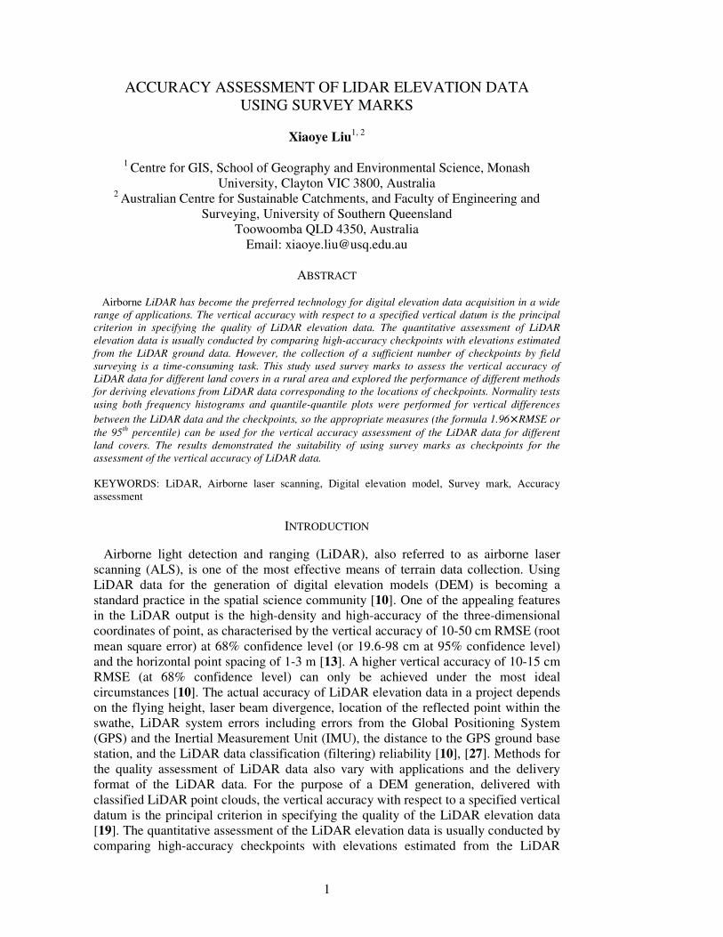
The study area is in the region of the Corangamite Catchment Management Authority (CCMA) in south western Victoria, Australia. The region features highlands in the north and south and the large Victorian Volcanic Plain (VVP) in the middle. The VVP is dominated by Cainozoic volcanic deposits and is characterised by vast open areas of grasslands, small patches of open woodland, stony rises denoting old lava flows, numerous volcanic cones and old eruptions, and dotted with shallow salt and freshwater lakes. The terrain types vary between the comparatively treeless basins of internal drainage on VVP to dissected terrains north and south. The plains have high priority for a range of research projects pertaining to environmental management issues addressed in the catchment management strategy plan. The study area, covered by LiDAR data from the first stage of the CCMA LiDAR project with the area of 6900 km² is shown in Figure 1.

Fig. 1. LiDAR data tiles and LiDAR data covered area

5

LIDAR DATA AND CHECKPOINTS

LiDAR data were collected using an Optech ALTM 3025 laser scanner from a fixed wing aircraft at flying heights of 2,000 m above ground from 19 July 2003 to 10 August 2003. The laser scanner was configured to record first and last returns with a frequency of 25 kHz (25,000 pulses per second). The laser footprint diameter at nadir is 0.6 m. The vertical accuracy of the LiDAR data was estimated as 0.5 m in terms of RMSE at 68% confidence level (or 0.98 m at 95% confidence level) for this project [1]. The primary purpose of this LiDAR data collection was to facilitate more accurate terrain pattern representation for the implementation of a series of environment related projects. The LiDAR data were separated into ground and non-ground points by using data filter algorithms across the project area. The manual checking and editing of the data led to a further improvement in the quality of the classification. The resulting data products used for the DEM generation are irregularly distributed ground 3D points, with an average spacing of 2.2 m [1]. The LiDAR data were delivered as tiles (5 km by 5 km) in ASCII files containing the x, y, z coordinates. The total of 277 LiDAR tiles is illustrated in Figure 1. The tiles on the project boundary contain LiDAR point data only inside the boundary. The LiDAR data covered area (project boundary) is shown in Figure 1 as well. Through the SMES, a total number of 199 survey marks which are located at ground level in the study area were obtained. All selected marks have 4th order or better vertical accuracy. The coordinates are based on the Map Grid of Australia 1994 (MGA94) and the Australian Height Datum (AHD).

METHOD

The general principle of assessing the vertical accuracy of a dataset is to compare the elevations obtained from the dataset with the reference data [5], so that statistical parameters such as the mean error, standard deviation or RMSE can be calculated to get an accuracy assessment of the results. For the vertical accuracy assessment of the LiDAR data, corresponding to the checkpoints, the LiDAR elevations are obtained from the LiDAR ground points. Except for the type of ground cover, the LiDAR data filtering process may also affect the accuracy assessment of the LiDAR data because some non-ground LiDAR points may not have been filtered out (and erroneously labelled as ground points). Therefore, ASPRS [2] requires open terrain to be tested separately from other ground types. There are four major land cover types in the study area: open terrain, weeds/crops, trees and residential areas. The number of checkpoints in each type of land cover is 80, 36, 36 and 47. The difference between each checkpoint’s elevation and the corresponding elevation from the LiDAR data can be calculated:

)()()( icheckidatai ZZZ −=∆ (1)

where )(icheckZ is the elevation of the ith checkpoint, and )(idataZ is the elevation from

the LiDAR data to be tested at the ith checkpoint. LiDAR ground points within a 10 m radius around each checkpoint were selected as a sub-dataset. The LiDAR elevation at the location of each checkpoint was derived from the sub-dataset. In this study, the TIN model, nearest point (NP) and cross validation methods were used to obtain the elevation from the sub-datasets. The first method is straightforward. A TIN was created for each of these sub-datasets. The elevation at the location of each checkpoint can be extracted from the TIN. The nearest LiDAR point was searched from each sub-dataset within a 3 m radius around the

6

checkpoint. The elevation of the LiDAR point closest to the checkpoint was then compared with the elevation of the checkpoint. The cross validation is another method for model evaluation. It removes one data point at a time and uses the remaining data points to predict the data value at the location of removed data point. The predicted and actual values at the location of removed data point are compared to assess the performance of interpolation methods. Here, the checkpoint was assumed to be the removed point in a sub-dataset. The ArcGIS Geostatistical Analyst Extension was used to carry out the cross validation. The result shows the elevation difference between the interpolated value and the checkpoint. The interpolated elevations at the location of each checkpoint may vary with the used interpolation algorithms. During the cross validation process, three commonly used interpolation algorithms, e.g. inverse distance weighting (IDW), Kriging and local polynomial (LP) were used to obtain elevations from the LiDAR sub-datasets. The results of accuracy assessment based on the interpolated elevations from the different interpolation algorithms were compared. The RMSE can be calculated from:

( )

n

ZZRMSE

n

i icheckidata∑ =−

= 1

2

)()( (2)

where n is the number of checkpoints used. If the elevation differences between the LiDAR data and the checkpoints follow a normal distribution, the overall vertical accuracy at the 95 percent confidence level can be calculated by using 1.96×RMSE [2]. In the case of a non-normal distribution, however, some robust measures such as the 95th percentile should be used for the accuracy assessment [2], [11]. A percentile is the interpolated absolute value in a dataset of errors, which divides the distribution of the individual errors in the dataset into one hundred groups of equal frequency [2]. The 95th percentile indicates that 95 percent of the errors in the dataset will have absolute values of equal or lesser value and 5 percent of the errors will be of a larger value. With this method, the accuracy is directly equated to the 95th percentile [2]. The elevation differences between the LiDAR data and the checkpoints in each of the four land cover categories and the combinations of land covers were tested using frequency histograms and quantile-quantile plots (or Q-Q plots) to see if they are normally distributed. The Q-Q plot is a scatter plot with the quantiles of the observed values on the horizontal axis and the expected normal values on the vertical axis. A dataset with a best-fit linear relationship indicates that the observed values are normally distributed [33].

RESULTS

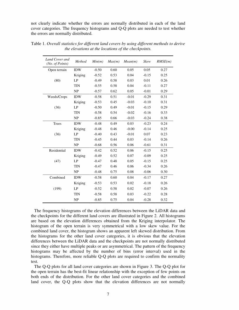
The overall descriptive statistics including the minimum, maximum and mean vertical errors, skew values, RMSE and the number of checkpoints used for each land cover category are listed in Table 1. The ranges between minimum and maximum errors vary mostly between -0.6 and 0.6 m for all land cover categories. The values outside this range only occurred when using the nearest point method to obtain elevations from the LiDAR data, indicating that the nearest point method may exaggerate the elevation errors. The mean generally also has the biggest absolute values when using the nearest point method. The RMSE values for the weeds/crops land cover are larger than for the other land cover categories irrespective of what methods were used for deriving the elevations from the LiDAR data. As a measure of the asymmetry of the probability distribution of a set, the skew values in Table 1 do

7

not clearly indicate whether the errors are normally distributed in each of the land cover categories. The frequency histograms and Q-Q plots are needed to test whether the errors are normally distributed. Table 1. Overall statistics for different land covers by using different methods to derive

the elevations at the locations of the checkpoints.

Land Cover and

(No. of Points) Method Min(m) Max(m) Mean(m) Skew RMSE(m)

Open terrain IDW -0.50 0.60 0.05 0.05 0.27

Kriging -0.52 0.53 0.04 -0.15 0.25

(80) LP -0.49 0.58 0.03 0.01 0.26

TIN -0.55 0.58 0.04 -0.11 0.27

NP -0.57 0.62 0.05 -0.01 0.29

Weeds/Crops IDW -0.58 0.51 -0.01 -0.29 0.31

Kriging -0.53 0.45 -0.03 -0.10 0.31

(36) LP -0.50 0.49 -0.01 -0.15 0.29

TIN -0.58 0.54 -0.02 -0.16 0.33

NP -0.85 0.66 -0.03 -0.24 0.38

Trees IDW -0.48 0.49 0.03 -0.23 0.24

Kriging -0.48 0.46 -0.00 -0.14 0.25

(36) LP -0.40 0.43 -0.01 0.07 0.23

TIN -0.45 0.44 0.03 -0.14 0.26

NP -0.68 0.56 0.06 -0.61 0.31

Residential IDW -0.42 0.52 0.06 -0.15 0.25

Kriging -0.49 0.52 0.07 -0.09 0.25

(47) LP -0.47 0.48 0.05 -0.15 0.25

TIN -0.47 0.46 0.06 -0.34 0.26

NP -0.48 0.75 0.08 -0.06 0.30

Combined IDW -0.58 0.60 0.04 -0.17 0.27

Kriging -0.53 0.53 0.02 -0.18 0.26

(199) LP -0.52 0.58 0.02 -0.07 0.26

TIN -0.58 0.58 0.03 -0.22 0.28

NP -0.85 0.75 0.04 -0.28 0.32

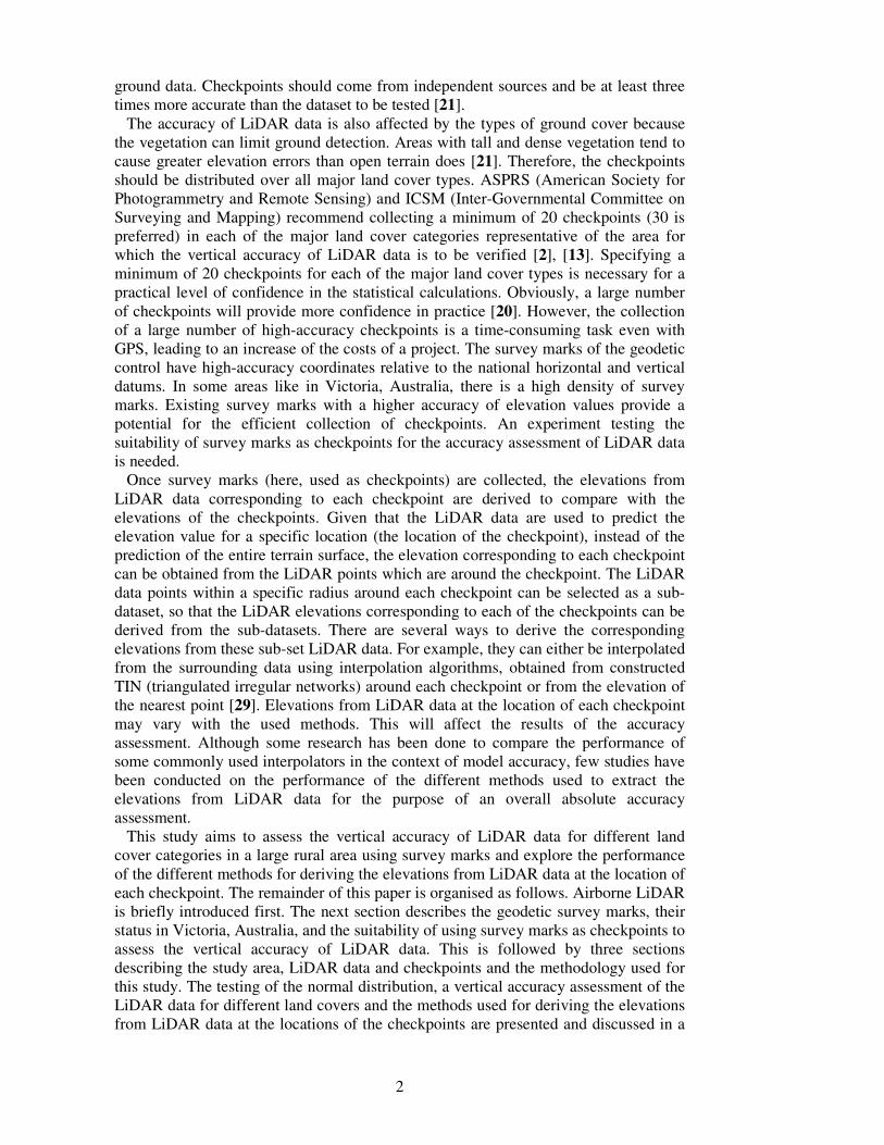
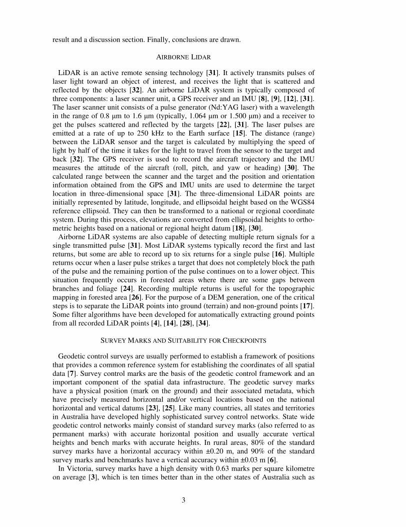
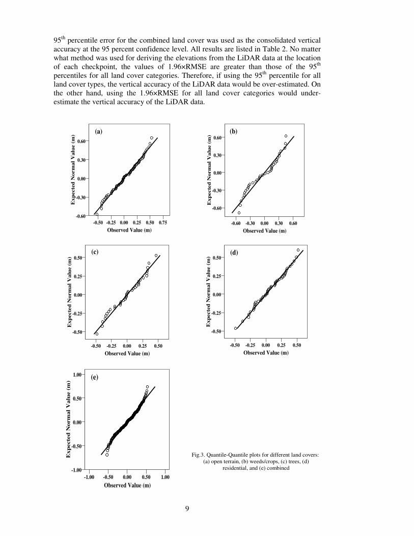
The frequency histograms of the elevation differences between the LiDAR data and the checkpoints for the different land covers are illustrated in Figure 2. All histograms are based on the elevation differences obtained from the Kriging interpolator. The histogram of the open terrain is very symmetrical with a low skew value. For the combined land cover, the histogram shows an apparent left skewed distribution. From the histograms for the other land cover categories, it is obvious that the elevation differences between the LiDAR data and the checkpoints are not normally distributed since they either have multiple peaks or are asymmetrical. The pattern of the frequency histograms may be affected by the number of bins (error interval) used in the histograms. Therefore, more reliable Q-Q plots are required to confirm the normality test. The Q-Q plots for all land cover categories are shown in Figure 3. The Q-Q plot for the open terrain has the best-fit linear relationship with the exception of few points on both ends of the distribution. For the other land cover categories and the combined land cover, the Q-Q plots show that the elevation differences are not normally

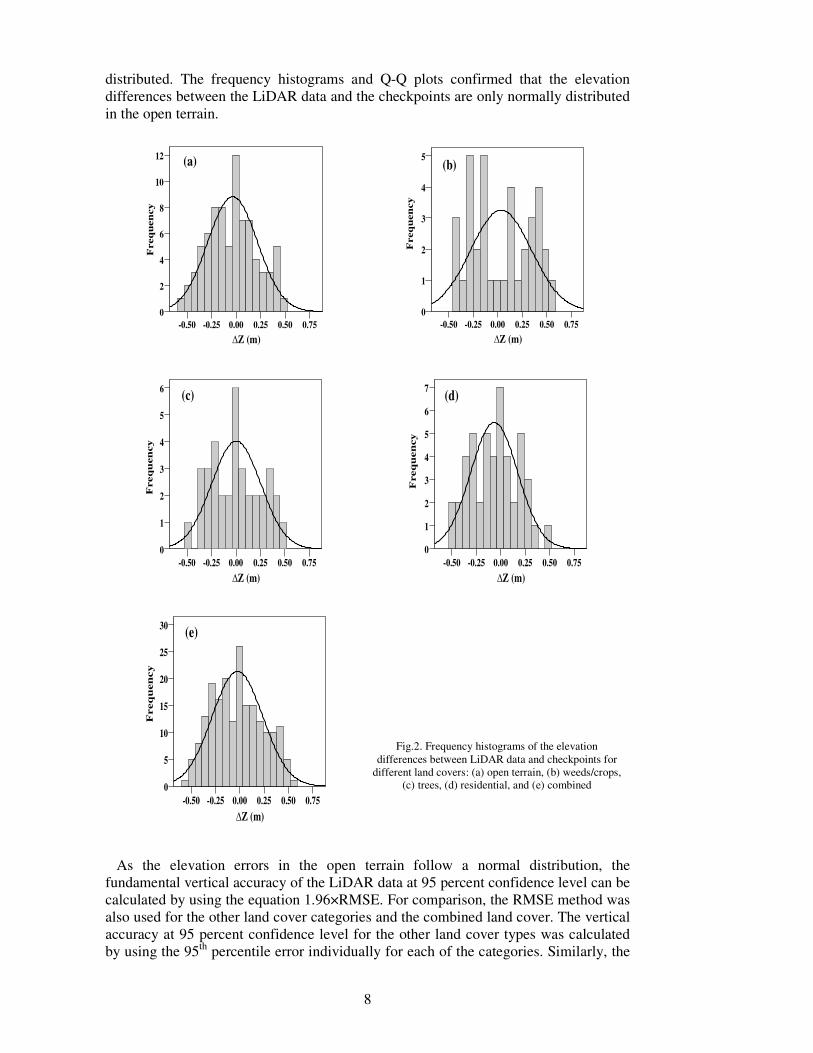
8

distributed. The frequency histograms and Q-Q plots confirmed that the elevation differences between the LiDAR data and the checkpoints are only normally distributed in the open terrain.

∆Z (m)

0.750.500.250.00-0.25-0.50

Freq

uen

cy

12

10

8

6

4

2

0

(a)

∆Z (m)

0.750.500.250.00-0.25-0.50

5

4

3

2

1

0

(b)

Freq

uen

cy

∆Z (m)

0.750.500.250.00-0.25-0.50

6

5

4

3

2

1

0

(c)

Freq

uen

cy

∆Z (m)

0.750.500.250.00-0.25-0.50

7

6

5

4

3

2

1

0

(d)F

req

uen

cy

∆Z (m)

0.750.500.250.00-0.25-0.50

30

25

20

15

10

5

0

(e)

Freq

uen

cy

Fig.2. Frequency histograms of the elevation differences between LiDAR data and checkpoints for

different land covers: (a) open terrain, (b) weeds/crops, (c) trees, (d) residential, and (e) combined

As the elevation errors in the open terrain follow a normal distribution, the fundamental vertical accuracy of the LiDAR data at 95 percent confidence level can be calculated by using the equation 1.96×RMSE. For comparison, the RMSE method was also used for the other land cover categories and the combined land cover. The vertical accuracy at 95 percent confidence level for the other land cover types was calculated by using the 95th percentile error individually for each of the categories. Similarly, the

9

95th percentile error for the combined land cover was used as the consolidated vertical accuracy at the 95 percent confidence level. All results are listed in Table 2. No matter what method was used for deriving the elevations from the LiDAR data at the location of each checkpoint, the values of 1.96×RMSE are greater than those of the 95th percentiles for all land cover categories. Therefore, if using the 95th percentile for all land cover types, the vertical accuracy of the LiDAR data would be over-estimated. On the other hand, using the 1.96×RMSE for all land cover categories would under-estimate the vertical accuracy of the LiDAR data.

Observed Value (m)

0.750.500.250.00-0.25-0.50

Exp

ecte

d N

orm

al

Valu

e (

m)

0.60

0.30

0.00

-0.30

-0.60

(a)

Observed Value (m)

0.600.300.00-0.30-0.60

Exp

ecte

d N

orm

al

Va

lue (

m)

0.60

0.30

0.00

-0.30

-0.60

(b)

Observed Value (m)

0.500.250.00-0.25-0.50

Ex

pecte

d N

orm

al

Valu

e (

m) 0.50

0.25

0.00

-0.25

-0.50

(c)

Observed Value (m)

0.500.250.00-0.25-0.50

Exp

ecte

d N

orm

al

Valu

e (

m) 0.50

0.25

0.00

-0.25

-0.50

(d)

Observed Value (m)

1.000.500.00-0.50-1.00

Ex

pecte

d N

orm

al

Va

lue (

m)

1.00

0.50

0.00

-0.50

-1.00

(e)

Fig.3. Quantile-Quantile plots for different land covers:

(a) open terrain, (b) weeds/crops, (c) trees, (d) residential, and (e) combined

10

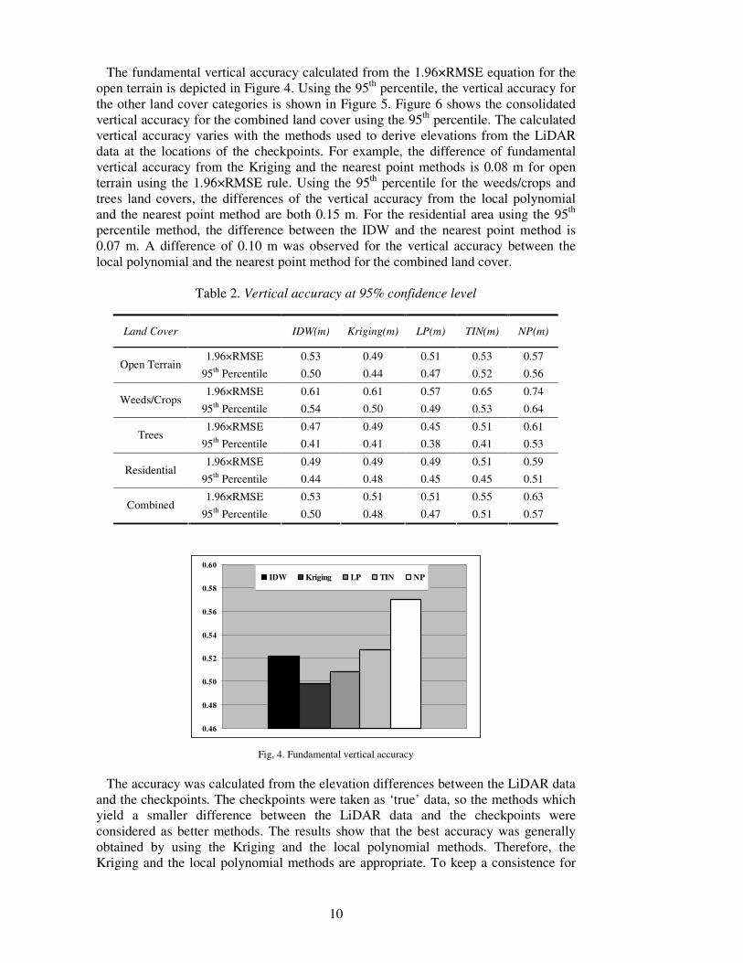
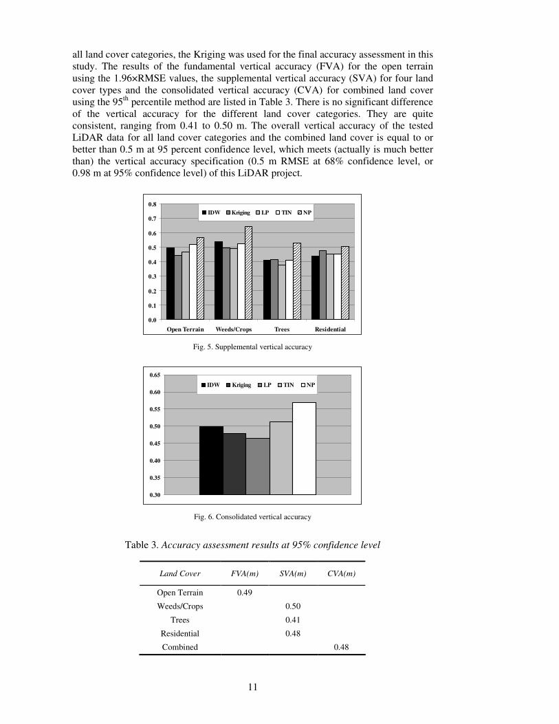
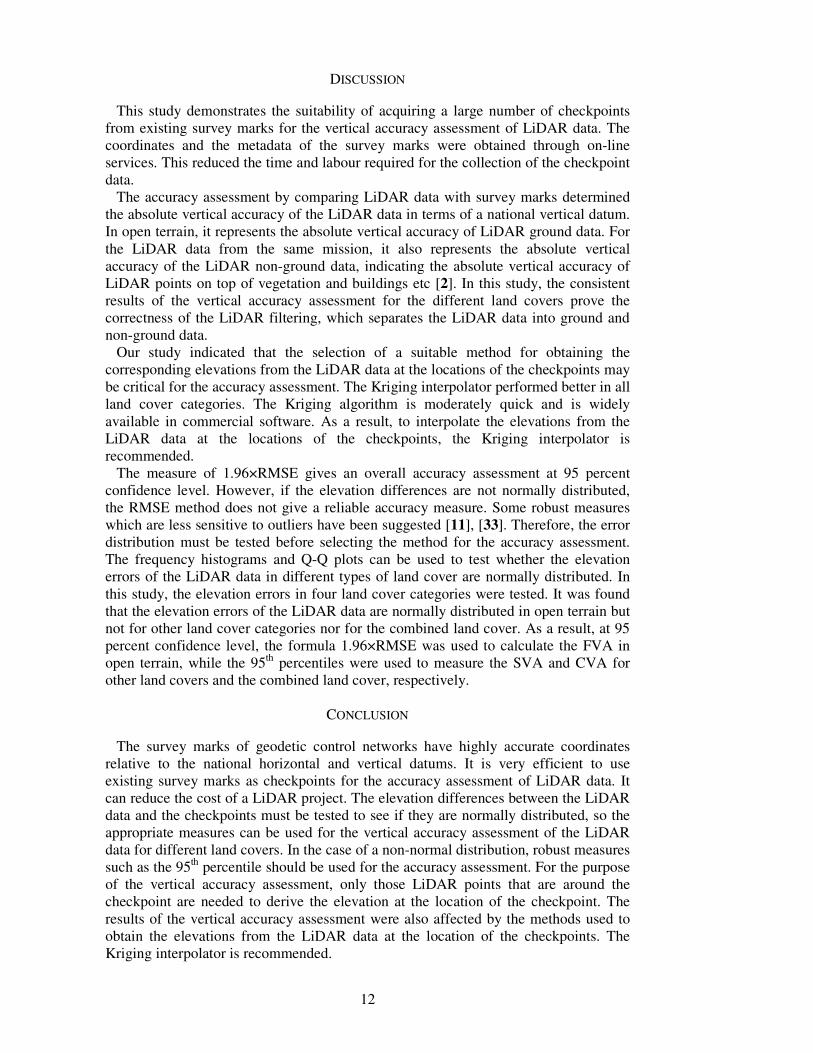
The fundamental vertical accuracy calculated from the 1.96×RMSE equation for the open terrain is depicted in Figure 4. Using the 95th percentile, the vertical accuracy for the other land cover categories is shown in Figure 5. Figure 6 shows the consolidated vertical accuracy for the combined land cover using the 95th percentile. The calculated vertical accuracy varies with the methods used to derive elevations from the LiDAR data at the locations of the checkpoints. For example, the difference of fundamental vertical accuracy from the Kriging and the nearest point methods is 0.08 m for open terrain using the 1.96×RMSE rule. Using the 95th percentile for the weeds/crops and trees land covers, the differences of the vertical accuracy from the local polynomial and the nearest point method are both 0.15 m. For the residential area using the 95th percentile method, the difference between the IDW and the nearest point method is 0.07 m. A difference of 0.10 m was observed for the vertical accuracy between the local polynomial and the nearest point method for the combined land cover.

Table 2. Vertical accuracy at 95% confidence level

Land Cover

IDW(m) Kriging(m) LP(m) TIN(m) NP(m)

1.96×RMSE 0.53 0.49 0.51 0.53 0.57 Open Terrain

95th Percentile 0.50 0.44 0.47 0.52 0.56

1.96×RMSE 0.61 0.61 0.57 0.65 0.74 Weeds/Crops

95th Percentile 0.54 0.50 0.49 0.53 0.64

1.96×RMSE 0.47 0.49 0.45 0.51 0.61 Trees

95th Percentile 0.41 0.41 0.38 0.41 0.53

1.96×RMSE 0.49 0.49 0.49 0.51 0.59 Residential

95th Percentile 0.44 0.48 0.45 0.45 0.51

1.96×RMSE 0.53 0.51 0.51 0.55 0.63 Combined

95th Percentile 0.50 0.48 0.47 0.51 0.57

0.46

0.48

0.50

0.52

0.54

0.56

0.58

0.60

IDW Kriging LP TIN NP

Fig, 4. Fundamental vertical accuracy

The accuracy was calculated from the elevation differences between the LiDAR data and the checkpoints. The checkpoints were taken as ‘true’ data, so the methods which yield a smaller difference between the LiDAR data and the checkpoints were considered as better methods. The results show that the best accuracy was generally obtained by using the Kriging and the local polynomial methods. Therefore, the Kriging and the local polynomial methods are appropriate. To keep a consistence for

11

all land cover categories, the Kriging was used for the final accuracy assessment in this study. The results of the fundamental vertical accuracy (FVA) for the open terrain using the 1.96×RMSE values, the supplemental vertical accuracy (SVA) for four land cover types and the consolidated vertical accuracy (CVA) for combined land cover using the 95th percentile method are listed in Table 3. There is no significant difference of the vertical accuracy for the different land cover categories. They are quite consistent, ranging from 0.41 to 0.50 m. The overall vertical accuracy of the tested LiDAR data for all land cover categories and the combined land cover is equal to or better than 0.5 m at 95 percent confidence level, which meets (actually is much better than) the vertical accuracy specification (0.5 m RMSE at 68% confidence level, or 0.98 m at 95% confidence level) of this LiDAR project.

0.0

0.1

0.2

0.3

0.4

0.5

0.6

0.7

0.8

Open Terrain Weeds/Crops Trees Residential

IDW Kriging LP TIN NP

Fig. 5. Supplemental vertical accuracy

0.30

0.35

0.40

0.45

0.50

0.55

0.60

0.65

IDW Kriging LP TIN NP

Fig. 6. Consolidated vertical accuracy

Table 3. Accuracy assessment results at 95% confidence level

Land Cover FVA(m) SVA(m) CVA(m)

Open Terrain 0.49

Weeds/Crops 0.50

Trees 0.41

Residential 0.48

Combined 0.48

12

DISCUSSION

This study demonstrates the suitability of acquiring a large number of checkpoints from existing survey marks for the vertical accuracy assessment of LiDAR data. The coordinates and the metadata of the survey marks were obtained through on-line services. This reduced the time and labour required for the collection of the checkpoint data. The accuracy assessment by comparing LiDAR data with survey marks determined the absolute vertical accuracy of the LiDAR data in terms of a national vertical datum. In open terrain, it represents the absolute vertical accuracy of LiDAR ground data. For the LiDAR data from the same mission, it also represents the absolute vertical accuracy of the LiDAR non-ground data, indicating the absolute vertical accuracy of LiDAR points on top of vegetation and buildings etc [2]. In this study, the consistent results of the vertical accuracy assessment for the different land covers prove the correctness of the LiDAR filtering, which separates the LiDAR data into ground and non-ground data. Our study indicated that the selection of a suitable method for obtaining the corresponding elevations from the LiDAR data at the locations of the checkpoints may be critical for the accuracy assessment. The Kriging interpolator performed better in all land cover categories. The Kriging algorithm is moderately quick and is widely available in commercial software. As a result, to interpolate the elevations from the LiDAR data at the locations of the checkpoints, the Kriging interpolator is recommended. The measure of 1.96×RMSE gives an overall accuracy assessment at 95 percent confidence level. However, if the elevation differences are not normally distributed, the RMSE method does not give a reliable accuracy measure. Some robust measures which are less sensitive to outliers have been suggested [11], [33]. Therefore, the error distribution must be tested before selecting the method for the accuracy assessment. The frequency histograms and Q-Q plots can be used to test whether the elevation errors of the LiDAR data in different types of land cover are normally distributed. In this study, the elevation errors in four land cover categories were tested. It was found that the elevation errors of the LiDAR data are normally distributed in open terrain but not for other land cover categories nor for the combined land cover. As a result, at 95 percent confidence level, the formula 1.96×RMSE was used to calculate the FVA in open terrain, while the 95th percentiles were used to measure the SVA and CVA for other land covers and the combined land cover, respectively.

CONCLUSION

The survey marks of geodetic control networks have highly accurate coordinates relative to the national horizontal and vertical datums. It is very efficient to use existing survey marks as checkpoints for the accuracy assessment of LiDAR data. It can reduce the cost of a LiDAR project. The elevation differences between the LiDAR data and the checkpoints must be tested to see if they are normally distributed, so the appropriate measures can be used for the vertical accuracy assessment of the LiDAR data for different land covers. In the case of a non-normal distribution, robust measures such as the 95th percentile should be used for the accuracy assessment. For the purpose of the vertical accuracy assessment, only those LiDAR points that are around the checkpoint are needed to derive the elevation at the location of the checkpoint. The results of the vertical accuracy assessment were also affected by the methods used to obtain the elevations from the LiDAR data at the location of the checkpoints. The Kriging interpolator is recommended.

13

ACKNOWLEDGEMENTS

The author would like to thank the anonymous reviewers and Editor-in-Chief for their comments and suggestions in improving the earlier version of this manuscript.

References 1. AAMHatch. 2003. Corangamite CMA Airborne Laser Survey Data Documentation, AAMHatch Pty Ltd,

Melbourne, Australia. 20 pages. 2. ASPRS. 2004. ASPRS Guidelines, Vertical Accuracy Reporting for LiDAR Data, American Society for

Photogrammetry and Remote Sensing (ASPRS), Bethesda, Maryland, USA. 20 pages. Available from: http://www.asprs.org/society/committees/lidar/Downloads/Vertical_Accuracy_Reporting_for_Lidar_Data.pdf

3. Bell, K. C., 2002. Annual Report by the Surveyor General of Victoria on the Administration of the Survey Co-

ordination Act 1958, Department of Sustainability and Environment, Melbourne, Australia. 15 pages. Available from: http://www.land.vic.gov.au/CA256F310024B628/0/B754484BCE358A1FCA257134000D27E7/$File/s20+SCA+2001-2002+Report.pdf

4. Chen, Q., 2007. Airborne LiDAR data processing and information extraction. Photogrammetric Engineering

and Remote Sensing, 73(2):109-112. 5. Congalton, R. G. and Green, K., 2009. Assessing the Accuracy of Remotely Sensed Data: Principles and

Practices. CRC Press, Boca Raton, London, New York. 183 pages. 6. DSE. 2004. Victoria's Geodetic Strategy (Incorporating a Strategic Maintenance Program for Ground Marks),

Department of Sustainability and Environment (DSE), Melbourne, Victoria, Australia. 42 pages. Available from: http://www.land.vic.gov.au/ca256f310024b628/0/b3297fb3cdae83e9ca2571250014213d/$file/geodetic+strategy+2004+oct.pdf

7. FGDC. 2008. Geographic Information Framework Data Content Standard, Part 4: Geodetic Control, Federal Geographic Data Committee (FGDC), Reston, Virginia. 23 pages. Available from: http://www.fgdc.gov/standards/projects/FGDC-standards-projects/framework-data-standard/GI_FrameworkDataStandard_Part4_GeodeticControl.pdf/view

8. Gomes Pereira, L. M. and Janssen, L. L. F., 1999. Suitability of laser data for DTM generation: a case study in the context of road planning and design. ISPRS Journal of Photogrammetry and Remote Sensing, 54(4):244-253.

9. Habib, A., Ghanma, M., Morgan, M. and Al-Ruzouq, R., 2005. Photogrammetric and LiDAR data registration using linear features. Photogrammetric Engineering and Remote Sensing, 71(6):699-707.

10. Hodgson, M. E. and Bresnahan, P., 2004. Accuracy of airborne lidar-derived elevation: empirical assessment and error budget. Photogrammetric Engineering and Remote Sensing, 70(3):331-339.

11. Höhle, J. and Höhle, M., 2009. Accuracy assessment of digital elevation models by means of robust statistical methods. ISPRS Journal of Photogrammetry and Remote Sensing, 64(4):398-406.

12. Hollaus, M., Wagner, W. and Kraus, K., 2005. Airborne laser scanning and usefulness for hydrological models. Advances in Geosciences, 5(1):57-63.

13. ICSM. 2008. ICSM Guidelines for Digital Elevation Data, Inter-Governmental Committee on Surveying and Mapping (ICSM), Canberra, Australia. 49 pages. Available from: http://www.icsm.gov.au/icsm/elevation/ICSM-GuidelinesDigitalElevationDataV1.pdf

14. Kraus, K. and Pfeifer, N., 1998. Determination of terrain models in wooded areas with airborne laser scanner data. ISPRS Journal of Photogrammetry and Remote Sensing, 53(4):193-203.

15. Lemmens, M., 2007. Airborne LiDAR sensors. GIM International, 21(2):24-27. 16. Lim, K., Treitz, P., Wulder, M. and Flood, B. S.-O. M., 2003. LiDAR remote sensing of forest structure.

Progress in Physical Geography, 27(1):88-106. 17. Liu, X., 2008. Airborne LiDAR for DEM generation: some critical issues. Progress in Physical Geography,

31(1):31-49. 18. Liu, X., Zhang, Z., Peterson, J. and Chandra, S., 2007. LiDAR-derived high quality ground control information

and DEM for image orthorectification. GeoInformatica, 11(1):37-53. 19. Maune, D. F., 2007. DEM User Requirements, in Maune, D. F. (Eds.), Digital Elevation Model Technologies

and Applications: The DEM Users Manual, 2nd Edition. American Society for Photogrammetry and Remote Sensing, Bethesda, Maryland. 449-473.

20. Maune, D. F., Maitra, J. B. and McKay, E. J., 2007. Accuracy Standards & Guidelines, in Maune, D. F. (Eds.), Digital Elevation Model Technologies and Applications: The DEM Users Manual, 2nd Edition. American Society for Photogrammetry and Remote Sensing, Bethesda, Maryland. 65-97.

21. NDEP. 2004. Guidelines for digital elevation data, Version 1.0, http://www.ndep.gov/NDEP_Elevation_Guidelines_Ver1_10May2004.pdf, National Digital Elevation Program (NDEP). (last date accessed: 18 January 2009).

22. Pfeifer, N. and Briese, C., 2007. Geometrical aspects of airborne laser scanning and terrestrial laser scanning. International Archives of Photogrammetry, Remote Sensing and Spatial Information Sciences, 36(3/W52):311-319.

14

23. Picco, J., Higgins, M., Sarib, R., Johnston, G. and Blick, G., 2006. Streamlining the exchange of geodetic data in Australia and New Zealand, Proc. of XXIII International FIG Congress, Munich, Germany. Available from: www.fig.net/pub/fig2006/papers/ts63/ts63_03_picco_etal_0502.pdf

24. Reutebuch, S. E., Andersen, H.-E. and McGaughey, R. J., 2005. Light detection and ranging (LIDAR): an emerging tool for multiple resource inventory. Journal of Forestry, 103(6):286-292.

25. RMIT. 2001. Review of the Cadastral Surveying Requirements of the Geodetic Surveying Infrastructure,

Consultants Report and Recommendations, Department of Geospatial Science, RMIT University, Melbourne, Australia. 63 pages. Available from: http://www.land.vic.gov.au/land/lcnlc2.nsf/9e58661e880ba9e44a256c640023eb2e/73bde2e0b00c60ffca257455001a4028/$file/attrh5bg/report.pdf

26. Sheng, Y., Gong, P. and Biging, G. S., 2003. Orthoimage production for forested areas from large-scale aerial photographs. Photogrammetric Engineering and Remote Sensing, 69(3):259-266.

27. Turton, D. A., 2006. Factors Influencing ALS Accuracy, AAMHatch Pty Ltd, Brisbane, Australia. 5 pages. 28. Vosselman, G., 2000. Slope based filtering of laser altimetry data. International Archives of Photogrammetry,

Remote Sensing and Spatial Information Sciences, 33(part B3/2):935-934. 29. Webster, T. L., 2005. LIDAR validation using GIS: a case study comparison between two LIDAR collection

methods. Geocarto International, 20(4):11-19. 30. Webster, T. L. and Dias, G., 2006. An automated GIS procedure for comparing GPS and proximal LiDAR

elevations. Computers & Geosciences, 32(6):713-726. 31. Wehr, A. and Lohr, U., 1999. Airborne laser scanning - an introduction and overview. ISPRS Journal of

Photogrammetry and Remote Sensing, 54(2-3):68-82. 32. Weitkamp, C., 2005. LiDAR: introduction, in Fujii, T. and Fukuchi, T. (Eds.), Laser Remote Sensing. Taylor &

Francis, Boca Raton, London, New York and Singapore. 1-36. 33. Zandbergen, P. A., 2008. Positional accuracy of spatial data: non-normal distributions and a critique of the

national standard for spatial data accuracy. Transactions in GIS, 12(1):103-130. 34. Zhang, K. Q., Chen, S. C., Whitman, D., Shyu, M. L., Yan, J. H. and Zhang, C. C., 2003. A progressive

morphological filter for removing nonground measurements from airborne LiDAR data. IEEE Transactions on

Geoscience and Remote Sensing, 41(4):872-882.