67

AC CircuitsUNIT 3 AC CIRCUITS

Structure 3.1 Introduction

Objectives

3.2 Sinusoidal Signals 3.2.1 Importance of Sinusoidal Signals 3.2.2 Effective Value and Form Factor 3.2.3 Phasor Representation

3.3 Impedance Concept 3.3.1 Response of Single Element to Sinusoidal Excitation 3.3.2 Concept of Impedance and Admittance 3.3.3 Mutual Inductance

3.4 Concepts Relating to Power 3.5 Three-phase Circuits

3.5.1 Nature of a 3-phase System 3.5.2 Merits of a 3-phase System 3.5.3 Characteristics of a 3-phase System 3.5.4 Star and Delta Connections

3.6 Summary 3.7 Answers to SAQs

3.1 INTRODUCTION

In Unit 2, we have studied Electromagnetism. The practical useful mode of storage of electrical energy at the present time is through DC storage batteries (rechargeable DC cells) and are widely used in transport vehicles, electronic instruments and equipment, portable tools, etc. However, the bulk of electrical energy utilisation, whether in domestic installations, or in industry or in public service organisations is through alternating current (AC) systems involving sinusoidal voltages and currents. Strictly speaking, the adjective alternating indicates any signal whose direction alternates with time but in practice, it is invariably used to refer to sinusoidal signals. In this Unit, you will first learn about the characteristics and representation of sinusoidal voltages and currents. You will then get to know the types of response of standard circuit elements to sinusoidal excitation. This will be a prelude to the study of methods of analysis of circuits formed by various combinations of simple circuit elements and operating under the influence of AC sources. The phasor concept which simplifies the expression of steady-state response-excitation relations in these circuits would be adopted as the framework for the development of the various techniques of analysis. You will also be introduced to the various ramifications of power in an AC circuit.

Objectives After studying this unit, you should be able to

• explain the reasons for the widespread use of sinusoidal signals in electrical engineering,

68

E/M Engineering

• deduce the different parameters of a sinusoidal waveform like peak value, phase, effective value, form factor etc.,

• work with complex numbers as needed for the manipulation of phasors in AC circuit analysis,

• express the steady state response both in time domain and in phasor domain of R, L, C elements to sinusoidal inputs,

• calculate the impedance Z and admittance Y of simple elements and combinations thereof in 2-terminal networks,

• explain the factors on which power in an AC circuit depends and distinguish between active power, apparent power and reactive power,

• describe characteristics of a 3-phase system,

• describe the features of a 3-phase system,

• distinguish between delta and star-connections of sources and loads, and

• distinguish between balanced and unbalanced systems.

3.2 SINUSOIDAL SIGNALS

Sinusoidal signals have a vital role both in electrical power engineering and in communication engineering. In power supply systems, the voltages and currents are invariably of this waveform with a frequency of 50 Hz in most countries including India. In the field of communication engineering, we have to deal with sinusoidal signals having wide frequency range extending from a few Hz to a few GHz (1 GHz = 109 Hz).

Formally, a sinusoidal function of time is defined as one having the general form and is characterised by three parameters viz., amplitude A, angular

frequency ω and phase angle θ. The argument (angle) of the sine function viz., )(sin θ+ωtA

)( θ+ωt is measured in radians and increases at the rate of ω radians per second. Since a sine function repeats itself at intervals of 2 π radians of its angle, we immediately see that the period T of the sinusoid is related to ω by π=ω 2T

We also know that the frequency f of the signal is the reciprocal of the period T. Therefore, we have

ff

π=ωπ=×ω 2or21

The parameters ω is, thus, a measure of the frequency of the signal and is called angular frequency. The phase angle θ is the value of the argument of the sine function at the origin of time and governs the instantaneous value at t = 0 of the sinusoidal signal of a given amplitude. Strictly speaking, θ should be expressed in radians as ωt is expressed in radians. However, since many of us have a better feel for angles measured in degrees, we often indulge in somewhat irregular practice of mixing up units by writing expressions like 325 sin (314 t + 60°)

instead of the more proper 325 sin .3

314 ⎟⎠⎞

⎜⎝⎛ π

+t However, the actual evaluation of

69

AC Circuitsthe sine function is done only after expressing the two terms in its argument in the

same units (radians or degrees) before their addition.

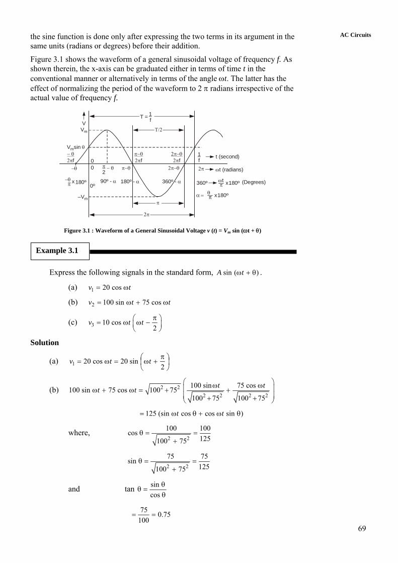
Figure 3.1 shows the waveform of a general sinusoidal voltage of frequency f. As shown therein, the x-axis can be graduated either in terms of time t in the conventional manner or alternatively in terms of the angle ωt. The latter has the effect of normalizing the period of the waveform to 2 π radians irrespective of the actual value of frequency f.

T/2

π

2π

T = 1fVVm

Vmsin θ− θ2πf 0

0

–Vm

π2

− θ π−θ 2π−θ

π−θ2πf

2π−θ2πf

1f

t (second)

2π ωt (radians)

0º

−θ

−θ 180º− π x 90º - α 180º - α 360º - α 360º ωtπ x180º (Degrees)

α = θπ x180º

Figure 3.1 : Waveform of a General Sinusoidal Voltage v (t) = Vm sin (ωt + θ)

Example 3.1

Express the following signals in the standard form, )(sin θ+ωtA .

(a) tv ω= cos201

(b) ttv ω+ω= cos75sin1002

(c) 3 10 cos2

v t t π⎛ ⎞= ω ω −⎜ ⎟⎝ ⎠

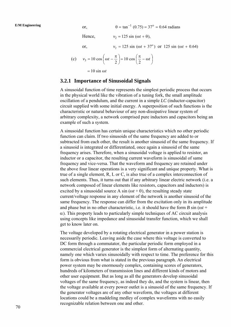
Solution

(a) ⎟⎠⎞

⎜⎝⎛ π

+ω=ω=2

sin20cos201 ttv

(b) 2 22 2 2 2

100 sin 75 cos100 sin 75 cos 100 75100 75 100 75

t tt t⎛ ⎞ω ω⎜ ⎟ω + ω = + +⎜ ⎟+ +⎝ ⎠

)sincoscos(sin125 θω+θω= tt

where, 2 2

100 100cos125100 75

θ = =+

2 2

75 75sin125100 75

θ = =+

and tan θθ

=θcossin

75.010075

==

70

E/M Engineering or, radians64.037)75.0(tan o1 ===θ −

Hence, 2 125 sin ( ),v t= ω + θ

or, 2 125 sin ( 37 ) 125 sin ( 0.64)orov t t= ω + ω +

(c) ⎟⎠⎞

⎜⎝⎛ ω−

π=⎟

⎠⎞

⎜⎝⎛ π

−ω= ttv2

cos102

cos103

tω= sin10

3.2.1 Importance of Sinusoidal Signals A sinusoidal function of time represents the simplest periodic process that occurs in the physical world like the vibration of a tuning fork, the small amplitude oscillation of a pendulum, and the current in a simple LC (inductor-capacitor) circuit supplied with some initial energy. A superposition of such functions is the characteristic or natural behaviour of any non-dissipative linear system of arbitrary complexity, a network comprised pure inductors and capacitors being an example of such a system.

A sinusoidal function has certain unique characteristics which no other periodic function can claim. If two sinusoids of the same frequency are added to or subtracted from each other, the result is another sinusoid of the same frequency. If a sinusoid is integrated or differentiated, once again a sinusoid of the same frequency arises. Therefore, when a sinusoidal voltage is applied to resistor, an inductor or a capacitor, the resulting current waveform is sinusoidal of same frequency and vice-versa. That the waveform and frequency are retained under the above four linear operations is a very significant and unique property. What is true of a single element, R, L or C, is also true of a complex interconnection of such elements. Thus, it turns out that if any arbitrary linear electric network (i.e. a network composed of linear elements like resistors, capacitors and inductors) is excited by a sinusoidal source A sin (ωt + θ), the resulting steady state current/voltage response in any element of the network is another sinusoid of the same frequency. The response can differ from the excitation only in its amplitude and phase but in no other characteristic, i.e. it should have the form B sin (ωt + α). This property leads to particularly simple techniques of AC circuit analysis using concepts like impedance and sinusoidal transfer function, which we shall get to know later on.

The voltage developed by a rotating electrical generator in a power station is necessarily periodic. Leaving aside the case where this voltage is converted to DC form through a commutator, the particular periodic form employed in a commercial electrical generator is the simplest form of alternating quantity, namely one which varies sinusoidally with respect to time. The preference for this form is obvious from what is stated in the previous paragraph. An electrical power system may be enormously complex, containing scores of generators, hundreds of kilometers of transmission lines and different kinds of motors and other user equipment. But as long as all the generators develop sinusoidal voltages of the same frequency, as indeed they do, and the system is linear, then the voltage available at every power outlet is a sinusoid of the same frequency. If the generator voltages are of any other waveform, the voltages at different locations could be a maddeling medley of complex waveforms with no easily recognizable relation between one and other.

71

AC CircuitsThe foregoing observations clearly highlight the importance of developing

efficient techniques for analysis of circuits under sinusoidal excitation. Further, these can be extended to find effective solutions for the behaviour of circuits and systems working under non-sinusoidal periodic and aperiodic excitations.

3.2.2 Effective Value and Form Factor The effective value of a periodic signal which counts power calculations are of concern and that for the particular case of a sinusoidal signal, the effective value

is ⎟⎟⎠

⎞⎜⎜⎝

⎛2

1 times the peak value. It is conventional to indicate the strength of a

sinusoidal voltage or current in terms of its effective value or Root Mean Square value (RMS value) and to simply use the capital letter V or I as the symbol for this quantity, discarding the subscripts in the symbols Veff and Ieff . A 230 V AC voltage would mean a voltage having an effective value of 230 V. This point has to be clearly understood that, unless otherwise stated, any numerical value assigned to an AC signal implies that it is the rms value and not either its peak value or its absolute average value. A 5 Amp, 50 Hz AC current would have a time variation θ)π100(sin52 +× t since the peak value is 2mI 5= × and

We hereafter indicate a general sinusoidal voltage and current as

2 (50) 100 .ω = π = π

θ)(sin2θ)(sin2 and +ω+ω tItV respectively, V and I being the corresponding effective values.

The only meaningful average value that can be associated with a sinusoid is the absolute average value (also equal to the average over the positive half cycle and hence called half-cycle average) and that the latter is equal to (2/π) times the peak value.

We now define the form factor of a symmetric periodic waveform as follows :

ValueAverageAbsolute

ValueRMSfactorForm = . . . (3.1)

From the name of the term, it is clear that form factor gives an indication of the shape of the wave. The sharper is the peak of the waveform, the larger is the form factor. For a flat waveform like the symmetrical square wave the form factor has a value equal to 1, since the RMS and absolute average values of this wave are equal. For a sinusoid, we have

Form factor of a sinusoid = 11.122π

)/π2(Value)(Peak2/ValuePeak

== . . . (3.2)

The form factor is a parameter to be considered in certain applications like the determination of the effective value of voltage induced in a coil due to changing magnetic flux of a given amplitude.

Example 3.2

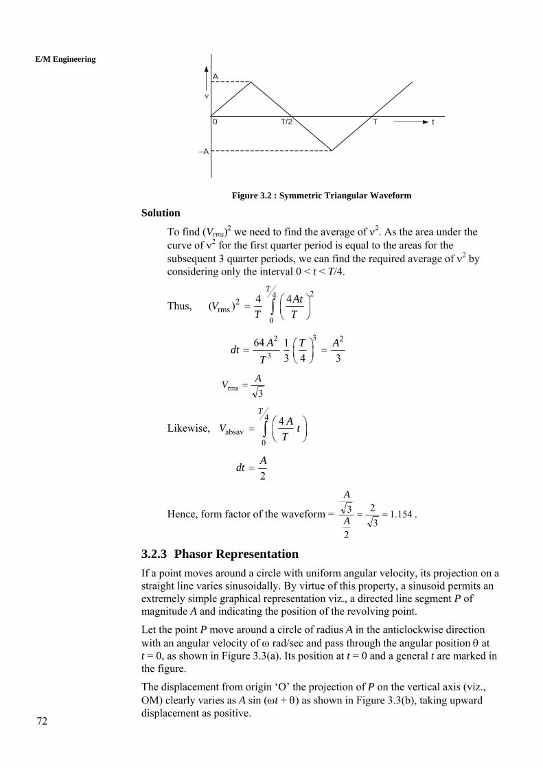
Find form factor of a symmetric triangular voltage waveform shown in Figure 3.2.

72

A

0 T/2 T

–A

ν

t

E/M Engineering

Figure 3.2 : Symmetric Triangular Waveform

Solution

To find (Vrms)2 we need to find the average of ν2. As the area under the curve of ν2 for the first quarter period is equal to the areas for the subsequent 3 quarter periods, we can find the required average of ν2 by considering only the interval 0 < t < T/4.

Thus, 24

2rms

0

4 4( )T

AtVT T

⎛ ⎞= ⎜ ⎟⎝ ⎠∫

32 2

364 1

3 4 3A T Adt

T⎛ ⎞= =⎜ ⎟⎝ ⎠

3rms

AV =

Likewise, 4

absav0

4T

AV tT

⎛ ⎞= ⎜ ⎟⎝ ⎠∫

2Adt =

Hence, form factor of the waveform = 154.13

2

2

3 ==A

A

.

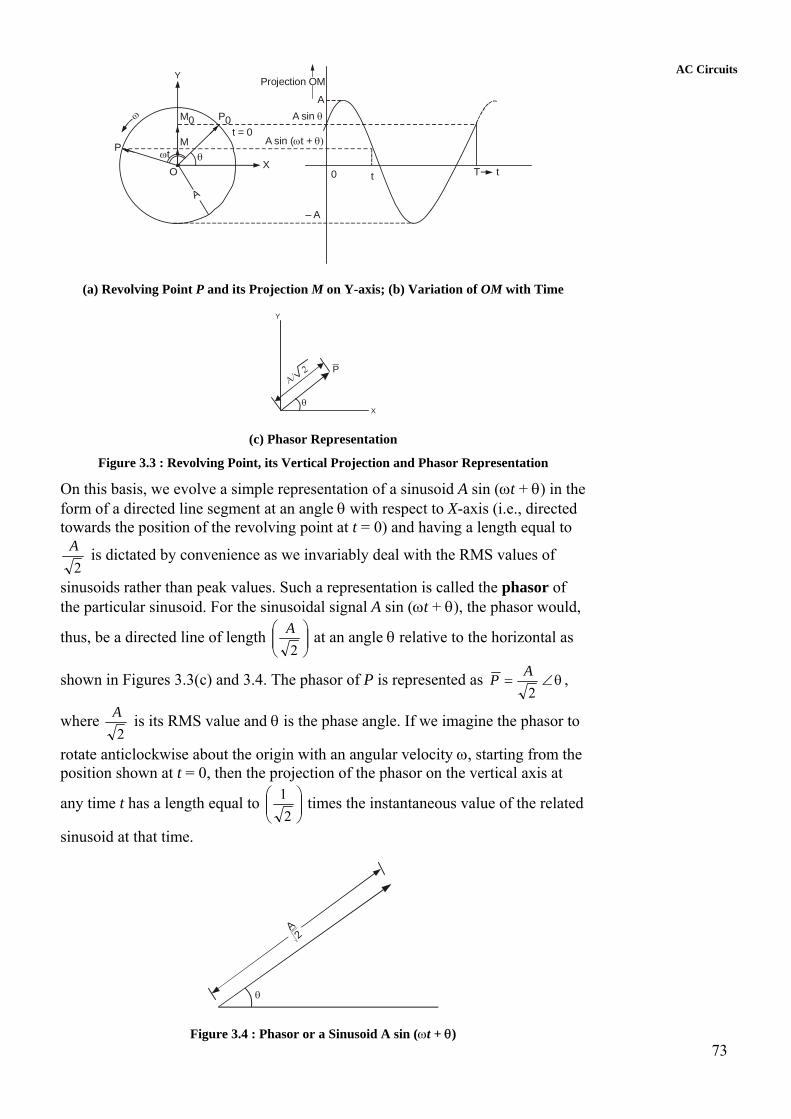
3.2.3 Phasor Representation If a point moves around a circle with uniform angular velocity, its projection on a straight line varies sinusoidally. By virtue of this property, a sinusoid permits an extremely simple graphical representation viz., a directed line segment P of magnitude A and indicating the position of the revolving point.

Let the point P move around a circle of radius A in the anticlockwise direction with an angular velocity of ω rad/sec and pass through the angular position θ at t = 0, as shown in Figure 3.3(a). Its position at t = 0 and a general t are marked in the figure.

The displacement from origin ‘O’ the projection of P on the vertical axis (viz., OM) clearly varies as A sin (ωt + θ) as shown in Figure 3.3(b), taking upward displacement as positive.

73

AC Circuits

O

ωt

A

M0

M

P0t = 0

P

ω

Y

Xθ

AA sin θ

A sin ( t + ω θ)

0 t tT

– A

Projection OM

(a) Revolving Point P and its Projection M on Y-axis; (b) Variation of OM with Time

Y

P

Xθ

(c) Phasor Representation

Figure 3.3 : Revolving Point, its Vertical Projection and Phasor Representation

On this basis, we evolve a simple representation of a sinusoid A sin (ωt + θ) in the form of a directed line segment at an angle θ with respect to X-axis (i.e., directed towards the position of the revolving point at t = 0) and having a length equal to

2A is dictated by convenience as we invariably deal with the RMS values of

sinusoids rather than peak values. Such a representation is called the phasor of the particular sinusoid. For the sinusoidal signal A sin (ωt + θ), the phasor would,

thus, be a directed line of length ⎟⎟⎠

⎞⎜⎜⎝

⎛2

A at an angle θ relative to the horizontal as

shown in Figures 3.3(c) and 3.4. The phasor of P is represented as θ∠=2

AP ,

where 2

A is its RMS value and θ is the phase angle. If we imagine the phasor to

rotate anticlockwise about the origin with an angular velocity ω, starting from the position shown at t = 0, then the projection of the phasor on the vertical axis at

any time t has a length equal to ⎟⎟⎠

⎞⎜⎜⎝

⎛2

1 times the instantaneous value of the related

sinusoid at that time.

A2

θ

Figure 3.4 : Phasor or a Sinusoid A sin (ωt + θ)

74

Any sinusoid is uniquely determined by three quantities viz., RMS value, frequency and phase. In AC circuit analysis, we normally deal with situations in which all currents and voltages have the same frequency and the value of this frequency is known. In this situation, one sinusoid differs from another only in respect of RMS value and phase, both of which are prominently displayed by a phasor. There is therefore a one-to-one correspondence between a sinusoid of a given frequency and its phasor and we can deduce one from the other. Different voltages and currents occurring in an AC circuit (operating with a single frequency excitation) can, therefore, be represented by an assembly of directed line segments having a common origin, a representation which is far more concise and clearer than a display of all the pertinent waveforms on a common time base. For example, the phase difference between two voltages is clearly visualized as the angle between the respective phasors. Several mathematical operations on phasors either graphically or analytically can be easily performed on phasors as we shall see in the subsequent sections.

E/M Engineering

As an example, consider two voltages νA = 220 sin (ωt + 30o) and )90(sin240 o+ω=υ tB with VA = 20 and VB = 40, whose waveforms are shown

in Figure 3.5(a). B

Volts

60º

60º 60º

60º

330º

360º180º

60º

0º-30º 270º

90º150º

ωt/(deg).

40 2

20 2

VB

VA 240º

60º

(a) Waveforms

60º30º

020 V

VB

40 VVA

ωt

(b) Phasors

Figure 3.5 : Two Sinusoids with a Phase Difference of 60o

75

AC CircuitsThe phase difference between νA and νB at an angular interval of 60 . νB

oB is said to

lead νA by 60 as successive similar events (e.g. upward zero crossings, positive peaks, negative peaks, downward zero crossings) occur with ν

o

BB at an angular interval of 60o earlier than with νA (Figure 3.5(a)). By the same token, νA is said to lag νB by 60 . B

o

This relationship between νA and νB can also be represented very simply with the help of phasors V

B

A and VBB as shown in Figure 3.5(b), which are supposed to rotate in anticlockwise direction with an angular speed ω. Thus, VB, which is moving ahead of V

B

A by exactly 60 is said to lead VoA by 60 . Similarly, Vo

A is said to lagging VBB by 60o. Thus, oo 90403020 and ∠=∠= BA VV and phase difference

.603090 ooo =−=

SAQ 1

Sketch the phasors of the following sinusoidal signals : (a) – 100 sin (ωt + 30o)

(b) )30(cos24 o+ωt

3.3 IMPEDANCE CONCEPT

In the previous section, we saw how the phasor concept provides an effective means of representing voltages and currents in AC circuits. In this section, we extend the application of this concept to characterisation of terminal relations of single elements and two-terminal networks. To this end, let us first examine the response of RLC elements to sinusoidal excitation.

3.3.1 Response of Single Element to Sinusoidal Excitation Resistance

Consider a resistor of R ohms connected to a sinusoidal voltage source of )(sin2 θ+ω= tVv volts as shown in Figure 3.6(a). From the fundamental

terminal relationship v = Ri of a resistor it follows that

i = (v/R) = )(sin)(2 θ+ωtV/R or )(sin2 θ+ω= tIi , where RVI = .

R

v+ –

iT

i, v

2 V 2 i

Vi

V/R

θ

V

IV

(a) Circuit (b) Waveform (c) Phasor Representation of IV and

Figure 3.6 : Response of a Resistor to Sinusoidal Excitation

We note the following : (a) The current and voltage are in phase (i.e., they have zero phase

difference). Both vary in step. The positive peaks, negative

76

peaks, zero crossing etc. occur in both at the same time as shown in Figure 3.6(b).

E/M Engineering

(b) RMS value of RVI = and, thus, the RMS values of voltage and

current are related by V = RI . . . (3.3)

a formula identical to Ohm’s law in DC domain.

(c) The voltage and current phasors being V V= ∠θ and VIR

⎛ ⎞= ∠θ⎜ ⎟⎝ ⎠

, as shown in Figure 3.6(c), they are related by

IRV = . . . (3.4)

Note that the above relationship is independent of ω and θ. Inductance

Now, let an inductor of L henrys have a voltage θ)(sin2 +ω=υ tV applied across it as shown in Figure 3.7. From the fundamental terminal relationship of an inductor, we have

dtL

idtdiL υ==υ ∫

1or

or dttVL

i )(sin21θ+ω= ∫

⎟⎠⎞

⎜⎝⎛ π

−+ωω

=+ωω

−=2

θsin2θ)(cos2 tLVt

LV

⎟⎠⎞

⎜⎝⎛ π

−+ω=2

θsin2 tI ,

where L

VIω

=

R

v+ –

i

(a) Circuit

i, v

2 V 2I

t

T/4

T/4

θ

V

I

V

90ºV

Lω

(b) Waveform (c) Phasor IV and

Figure 3.7 : Response of an Inductor to Sinusoidal Excitation

77

AC CircuitsWe take the constant of integration in the above to be zero as for the AC

circuits of concern to us, there cannot be a DC or constant current in any element.

The main characteristics of this response are : (a) The current has phase difference of 90o with respect to the

voltage and lags behind it. Similar events (positive peaks, negative peaks, upward zero crossings, downward zero crossings etc.) occur in the voltage wave a quarter-period (equivalent to 90o of the angle ωt) earlier than the current wave, as shown in Figure 3.7.

(b) RMS value of L

VIω

= , and, thus, the RMS values of voltage

and current are related by V = (ωL) I . . . (3.5)

(c) The phasors of v and i being ⎟⎠⎞

⎜⎝⎛ −∠=∠=

2πθandθ IIVV

They are related by

ILjV )( ω= . . . (3.6)

where, j is 90o operator. Capacitance

Figure 3.8 shows a capacitor of C farads applied with a voltage ).(sin2 θ+ω=ν tV The current through the capacitor would, therefore,

be

( 2 sin )dv di C C V tdt dt

= = ω + θ

⎟⎠⎞

⎜⎝⎛ π

+θ+ωω=θ+ωω=2

sin2)(cos2 tCtVC

⎟⎠⎞

⎜⎝⎛ π

+θ+ω=2

sin2 tI ,

where VCI ω=

The main characteristics of this response are : (a) The current has a phase difference of 90o with respect to the

voltage and leads the latter. Similar events occur in the current wave a quarter-period (equivalent to 90o) earlier than the voltage wave as shown in Figure 3.8.

(b) Since RMS value of current VCI ω= , the RMS values of voltage and current are related by

IC

V ⎟⎟⎠

⎞⎜⎜⎝

⎛ω

=1 . . . (3.7)

(c) The phasors V and I being and2

V CV π⎛ ⎞∠ θ ω ∠ θ +⎜ ⎟⎝ ⎠

respectively, they are related by

ICj

Vω

=1 . . . (3.8)

78

The properties derived earlier are characteristic of the three elements in AC circuits and hold irrespective of where they are connected in a circuit. A little reflection will show that item (c) in each case is a complete statement of the relevant properties and incorporates in itself the properties specifically stated under (a) and (b).

E/M Engineering

C

ν+ –

i

2 V2I

t

T/4

T/4

i V

I

90ºV

V

θωCV

(a) (b) (c)

Figure 3.8 : Response of a Capacitor to Sinusoidal Excitation

To summarise, the three elements R, L and C respond differently to sinusoidal excitations (current or voltage). The current and voltage in a resistor are in phase, while they are in quadrature (i.e., have a phase difference of 90o) in an inductor or a capacitor. In an inductor, the voltage leads the current by 90o while in a capacitor, the current leads the voltage by 90o. The RMS values of the voltage across and the current through the element satisfy the proportionality relationship given in each case by Eqs. (3.3), (3.5) and (3.7) respectively. For a given value of current to be driven through it, an inductor requires more voltage as the frequency increases. The capacitor on the other hand, needs only a smaller voltage as the frequency increases.

Example 3.3

A capacitor draws a current of 5 mA from 200 V, 50 Hz AC supply. What current does it draw from 40 V, 400 Hz supply?

Solution

As mentioned earlier, all values relating to voltages and currents in AC circuit are to be taken as RMS values unless specifically stipulated otherwise, we have

VCI ω=

for a given C,

6.120040

50400.

1

2

1

2 =×=ωω

=1

2VV

II

or mA8mA56.16.1 12 =×== II

Hence, the current with 40 V, 400 Hz supply = 8 mA.

79

AC Circuits

SAQ 2

(a) Fill in the blanks :

In a capacitor the current . . . . . . . . . . . . . . . . . . . . . . . . the voltage by . . . . . . . . . . . . . . . . . . . . degrees, while in a . . . . . . . . . . . . . . . . . . . . . it is in phase with voltage. For a given applied voltage an inductor permits a . . . . . . . . . . . . . . . . . . . . . current as the frequency is raised.

(b) Find the inductance of an inductor which draws a current of 1.1A when connected to 230 V, 50 Hz voltage. What current will it draw if the supply voltage is changed to 150V, 25 Hz?

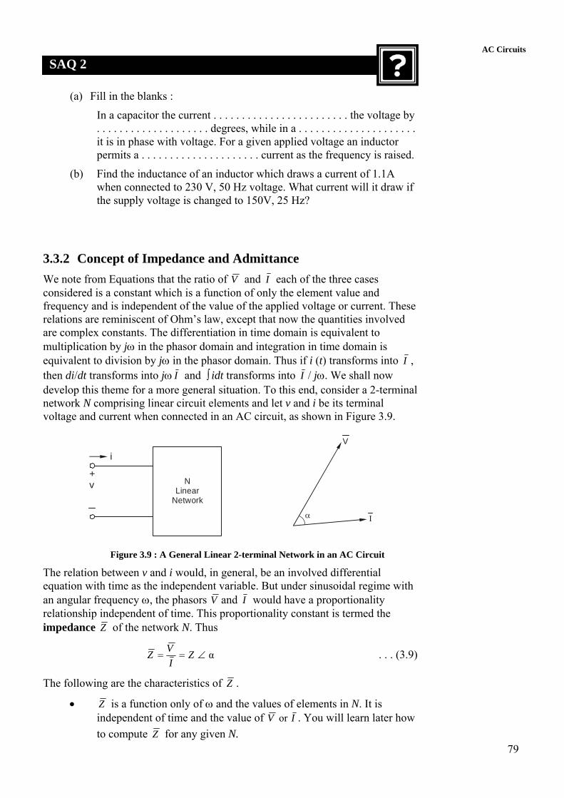
3.3.2 Concept of Impedance and Admittance We note from Equations that the ratio of V and I each of the three cases considered is a constant which is a function of only the element value and frequency and is independent of the value of the applied voltage or current. These relations are reminiscent of Ohm’s law, except that now the quantities involved are complex constants. The differentiation in time domain is equivalent to multiplication by jω in the phasor domain and integration in time domain is equivalent to division by jω in the phasor domain. Thus if i (t) transforms into I , then di/dt transforms into jω I and idt transforms into ∫ I / jω. We shall now develop this theme for a more general situation. To this end, consider a 2-terminal network N comprising linear circuit elements and let v and i be its terminal voltage and current when connected in an AC circuit, as shown in Figure 3.9.

NLinear

Network

+v

i

α I

V

Figure 3.9 : A General Linear 2-terminal Network in an AC Circuit

The relation between v and i would, in general, be an involved differential equation with time as the independent variable. But under sinusoidal regime with an angular frequency ω, the phasors V and I would have a proportionality relationship independent of time. This proportionality constant is termed the impedance Z of the network N. Thus

α∠== ZIVZ . . . (3.9)

The following are the characteristics of Z .

• Z is a function only of ω and the values of elements in N. It is independent of time and the value of IV or . You will learn later how to compute Z for any given N.

80

E/M Engineering

• Z has the same dimensions as resistance and is measured in Ω.

• From the definition of Z , we have IZV = . . . (3.10)

which plays the same role in AC circuits as Ohm’s law in DC circuits.

• The magnitude Z for the impedance is the ratio of the effective values of voltage and current. Sometimes, Z itself is referred to as the impedance instead of Z .

• α is called the angle of the impedance Z and denotes the phase angle by which V leads I .

• In rectangular coordinate form, Z can be expressed as XjR +=Z ,

where the real and imaginary components R and X are respectively called the effective resistance and reactance of N, the latter may, in general, be positive or negative, but for a network N comprising no active elements (e.g., dependent sources), R is always non-negative

• Z is to be viewed purely as a complex number and cannot be associated with any sinusoidal signal as its phasor.

Note : We should distinguish between a physical element and its circuit parameter. But expressions like a resistor having a resistance of 20 Ω is connected in parallel with a capacitor of 1 μF capacitance are not only inconvenient but may even sound pedantic. Hence, you often find in literature an element itself being referred to by its circuit parameter – resistance, inductance or capacitance. Thus, the previous expression would usually be rewritten “a 20 Ω resistance is connected in parallel with a 1 μF capacitance”. We may call the two-terminal network N itself as the impedance Z .

As a dual concept to impedance, we define the admittance Y of the network N as

β∠== YVIY . . . (3.11)

Obviously Y is reciprocal to Z , is measured in Siemens and enables determination of current for a given applied voltage by

VYI = . . . (3.12)

also, Y = Z − 1 and β = − α.

In rectangular coordinate form, Y may be expressed as ,jBGY +=

where G and B are referred to as the effective conductance and susceptance of N. Let us now discuss the behaviour of single elements.

From Equation and the definition of Z , we deduce the following expressions for the impedance.

Element Resistance (R)

Inductance (L)

Capacitance (C)

Impedance Z R jωL = jXL 1/jωC = − j/ωC = − jXC

81

AC CircuitsThe impedance of a resistor is purely real, equal to its resistance R and has no

imaginary component. It is in anticipation of this that we have used the symbol R for the real part of Z . On the other hand, inductors and capacitors have purely imaginary impedances, inductive reactance XL being positive and capacitive reactance (− XC) being negative.

How does one calculate the impedance of a network with several elements? To obtain a clue, let us consider a series combination of several sub-networks with impedances nZZZ ,...,, 21 as shown in Figure 3.10.

When an AC current having I for its phasor passes through the series combination, we have

IZVIZVIZV nn === ,...,, 2211

V+

a

b

V1

Z1

V2

Z2

V3

Z3

Vn

Zn

I

+ + + +

–

– – – –

Figure 3.10 : Series Combination of Impedances

Using KVL in phasor form, the terminal voltage of the combination is

IZZZIZIZVVVV nnn )...(...... 21121 +++=++=+++=

Thus, the equivalent impedance of the series combination is

1 2 . . .s nZ Z Z Z= + + + . . . (3.13)

In a similar fashion, it is left to the reader to show using KCL that the equivalent impedance and admittance of the parallel combination shown in Figure 3.11 are given by

np ZZZZ

1...111

21

+++= . . . (3.14(a))

or nP YYYY +++= ...21 . . . (3.14(b))

I

V

+

–

I1

Y1 Y2I2

YnIn

Figure 3.11: Parallel Combination of Admittances Eqs. (3.13) and (3.14) are similar to rules for combining resistors in series and in parallel. We will encounter a similar pattern in future. All the techniques that we have learnt for DC circuit analysis can be applied to AC circuits as well with certain modifications. The techniques include finding series-parallel equivalents,

82

current and voltage division rules, star-delta conversions, loop circuit and node voltage analyses etc. The departure from DC methods are :

E/M Engineering

• KVL and KCL relations are expressed in phasor form.

• Impedance Z (or admittanceY ) is used in place of resistance (or conductance),

• Terminal relations VYIIZV == and are used instead of V = RI and I = GV in DC domain.

This is the power and beauty of the phasor concept. Essentially, the same methods and formulations applicable to circuits with constant currents and voltages are made applicable to circuits with currents and voltages varying in time sinusoidally. The price we have to pay for this simplification, namely dealing with complex numbers, is indeed less taxing than the alternative of working in time domain with trigonometric functions and carrying out differentiation and integration operations thereof.

Example 3.4

Find the impedance of the element combinations shown in Figure 3.12, taking the frequency to be 400 Hz.

20 Ω 10 Fμ 10 mH100 Ω

(a) (b)

40 Ω

5 Fμ

(c)

60 Ω

20 mH

(d)

Figure 3.12

Solution (a) The impedance of the series combination is the sum of the two

impedances.

1 2 6120

2 400 10 10sZ Z Zj −

= + = +π × × ×

= 20 – j 39.8 Ω

(b) 31 2 100 2 400 100 10sZ Z Z j −= + = + π × × ×

= 100 + j 251 Ω (c) Alternative I

1 2 6140 ; 79.6

2 400 5 10Z Z j

j −= Ω = = −

π × × ×Ω

The two impedances being in parallel,

o

1 2o

1 2

40 ( 79.6) 3184 9040 79.6 89.1 63.3

rZ Z jZ

Z Z j− ∠

= = =+ − ∠ −

−

= 35.7∠ – 26.7o = 31.9 – j 16.0 Ω

Alternative II

83

AC Circuits

61 2

1 0.02 ; 2 400 5 10 0.0126 .40

Y S Y j C j j−= = = ω = π × × × = S

The two admittances being in parallel,

oP jYYY 7.26028.00126.0025.021 ∠=+=+=

Then

Ω−=−∠=∠== −− 0.169.317.267.35)7.26028.0()( 11 jYZ ooPP

(d) Ω+=∠=∠∠

= 5.297.24505.38403.78903018 jZ o

o

o

P

Example 3.5

When the element combination in Figure 3.12(a) is connected to 200 V, 400 Hz supply, what would be the current drawn? What would be the voltage across the resistance and capacitance?

Solution As the phase of the supply voltage is not specified, we need to compute only the RMS value of the current. Z = (202 + 39.82)1/2 = 44.54 Ω I = V/Z = 200 / 44.54 = 4.49 A VR = IR = 4.49 × 20 = 89.8 V VC = (I / ωC) = 4.49 × 39.8 = 178.7V

Example 3.6

If a voltage of 200 V, 400 Hz is applied across the element combination in Figure 3.12(c), find the total current taken by the combination.

Solution Since the phase of the supply voltage has not been specified, let us take it as 0o. That is, we are taking the applied voltage phasor as the so-called reference phasor. oV 0200 ∠=

Now 540/200/0200 o ==∠= RIR

and 52.2)900126.0()0200( oo jCjVIC =∠∠=ω=

A6.5)52.25(52.25 2/122 =+=⇒+=+= IjIII CR

The phasor diagram showing the relative positions of the different phasors is given in Figure 3.13.

I

IR

IC

+ V

IC I

IR

V Figure 3.13

84

If V has any other phase angle say αo it only means that the entire figure will rotate by αo. There will be no change in the magnitudes of the voltages and currents and in their phase differences. This is an important point to note. When no contrary information is specified, we are at liberty to arbitrarily assume one convenient quantity as the reference phasor.

E/M Engineering

3.3.3 Mutual Inductance The property of an inductance coil is to set up a magnetic field when carrying a current. Some of the magnetic flux lines so set up may also link with another coil (inductor) in its proximity. In such an event, the two coils are said to be magnetically coupled. When the current in the first coil changes, not only do its self flux linkages change but also the flux linkages (called mutual flux linkages) produced by it in the second coil. Consequently, there is a voltage induced in the second coil due to a change of current in the first coil. The action described above is reciprocal in that a change of current in the second coil would also induce a proportionate voltage in the first coil. The induced voltage in each coil is produced due to per unit rate of change of current in the other and is defined to be the mutual inductance M between the coils. M is another passive circuit parameter like R, L and C that we discussed in Unit 1 and arise whenever two inductors are coupled magnetically. It is measured in the same units as L viz., henrys. The principle of mutually induced voltage forms the basis of transformer action.

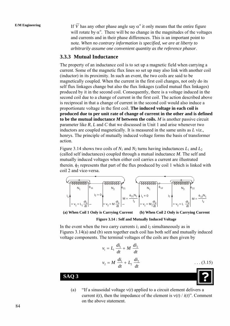
Figure 3.14 shows two coils of N1 and N2 turns having inductances L1 and L2 (called self inductances) coupled through a mutual inductance M. The self and mutually induced voltages when either coil carries a current are illustrated therein. φ2 represents that part of the flux produced by coil 1 which is linked with coil 2 and vice-versa.

i1 = 0M =

φ21 2N

i2+ v1 = M1

didt

2

ρφ12

i2

N1 N2

+ v2 = Ldidt

2

ρφ22

M =φ12 1N

i2

N1

ρφ11

ρφ21

i1

+ v1 = L1didt

1 + v2 = Mdidt

1

N2

i 2 = 0

–– (a) When Coil 1 Only is Carrying Current (b) When Coil 2 Only is Carrying Current

Figure 3.14 : Self and Mutually Induced Voltage

In the event when the two carry currents i1 and i2 simultaneously as in Figures 3.14(a) and (b) seen together each coil has both self and mutually induced voltage components. The terminal voltages of the coils are then given by

dtdiM

dtdiLv 21

11 +=

dtdiL

dtdiMv 2

21

2 += . . . (3.15)

SAQ 3

(a) “If a sinusoidal voltage ν(t) applied to a circuit element delivers a current i(t), then the impedance of the element is ν(t) / i(t)”. Comment on the above statement.

85

AC Circuits(b) Fill up the following table

Element Resistance (R)

Inductance (L)

Capacitance(C)

Admittance Y

SAQ 4

(a) In Example 3.5, VR and VC do not add up to the magnitude of the supply voltage. Is this not a violation of KVL?

(b) If a current i (t) = 2 sin (400 t + 30o) mA passes through the element combination in Figure 3.12(b), find an expression for the voltage across the combination.

SAQ 5

(a) A resistance of 20 Ω and an impedance 40 + j 60Ω are connected

across an AC supply source as shown in Figure 3.15. If the voltage across the resistor is 50 V, find the source voltage. Draw a phasor diagram.

40 + j60 Ω20 Ω

Figure 3.15

(b) A fluorescent lamp may be considered to be a pure resistance. A 40 W lamp is designed to operate at a voltage of 130 V at 50 Hz. This lamp, in series with a choke coil (which may be considered a pure inductor), is connected across 220 V, 50 Hz supply. Calculate the required value of inductance of the choke coil.

3.4 CONCEPTS RELATING TO POWER

Since AC circuits have periodically varying voltages and currents, the power delivered to an element or a section of a circuit is also a periodically varying

86

quantity p(t). A meaningful measure of power in such situations is the average power over a cycle. The term power when used in the context of an AC circuit without any additional qualification means this average value and is denoted by the symbol P. In a DC circuit, the power delivered to a 2-terminal network is equal to VI, the product of the terminal voltage and current. In what follows, we develop the corresponding formula applicable to AC circuits.

E/M Engineering

3.4.1 Power, Apparent Power and Power Factor Consider the circuit given in Figure 3.16, where sinusoidal voltage

2 V sin ( t )v = ω + θ supplies power to a 2-terminal network N having an equivalent impedance .jXRZZ +=∠= α In this context, N is also referred to as a load and Z as the load impedance.

i

~+

v = 2 V sin ( t + )ω θ

N

Z ∠ α θα

I

V

Figure 3.16

The phasor I of the resultant current I in this circuit is

α)(θ −∠⎟⎠⎞

⎜⎝⎛=⎥

⎦

⎤⎢⎣

⎡α∠θ∠

=ZV

ZVI

Thus )(sin2)(sin2 α−θ+ω=α−θ+ω⎟⎠⎞

⎜⎝⎛= tIt

ZVI

The instantaneous power supplied by the source to the load is

)(sin2.)(sin2)( α−θ+ωθ+ω=υ= tItVitP

)(sin)(sin2 α−θ+ωθ+ω= ttIV

)]22(cos[cos α−θ+ω−α= tIV

The variation of p(t) is shown in Figure 3.17.

α

θ

v, i, p

VI

pv

i

P = Avg. of p(t) = VI cos α

ωt

87

AC CircuitsFigure 3.17 : Instantaneous Power p(t) Delivered to N

It is seen from Figure 3.17 (hatched portion) that p(t) consists of a constant component V I cos α second component of peak value V I varying sinusoidally at a frequency 2ω. As the average of the second component over a period of the input voltage or current is zero, the average of p(t) is equal to the first component itself. Thus,

P = V I cos α Watts . . . (3.16)

The above formula is of great significance. It indicates that the power received by a load is not merely the product of the RMS values of its terminal voltage and current but includes an additional multiplicative factor cos α, called the power factor of the load. Power factor is the cosine of the impedance angle α and hence is a property of the concerned load. Formally, power factor (p.f.) may be defined as

Power deliver to loadp.f.Product of effective values of terminal voltage and current of the load

=

p.f. PVI

= . . . (3.17)

The power factor is said to be of the leading type if I leads V (i.e., X < 0) and of the lagging type if I lags V (i.e. X > 0).

In contrast to power P, the product VI is termed apparent power S and is indicated in units of volt-amperes (abbreviated VA). Though dimensionally 1 VA equals 1 Watt, two different names of the unit are adopted to emphasize the distinct between apparent power S and P. Apparent power is an important parameter in the specifications of electrical equipment, as the size and cost of many electrical machines depend on their VA rating rather than wattage rating. For instance, a 500 kVA distribution transformer is rated in terms of its ability to handle S up to 500 kVA level which determines maximum current at rated voltage rather than power P it can deliver to a load which in dependent on load power factor.

Table 3.1 gives the particular forms of the relations discussed above for special categories of loads. Note that a pure inductor and capacitor have zero p. f. since they are only energy storage elements and not energy dissipating elements.

Table 3.1

Load Z (Ω)

α Apparent Power (S) (VA)

Power Factor Power (P) (W)

Resistor R 0o VI = I 2 R = V 2/R 1.0 (unity) VI = I 2 R = (V 2/R) Inductor j ω L 90o VI = I 2 ω L = (V 2/ω L) Zero (lagging) Zero

Capacitor 1/j ω C − 90o VI = I 2 / ω C = (V 2 ω C) Zero (leading) Zero

3.5 THREE-PHASE CIRCUITS

A sinusoidal voltage source with 2 terminals having a single voltage output is termed a single-phase source. Circuits incorporating such sources are called single phase (1-phase) circuits and formed the subject of our study uptil now in this unit. In contrast, a poly-phase system contains sources each of which has several voltage outputs with a fixed phase difference between them. The three-

88

phase (3-phase) system is the most common example of a poly-phase system.

E/M Engineering

The generation and transmission of electrical energy and its utilization in bulk form is effected through 3-phase systems. You will learn about the precise nature of a 3-phase system and the advantages it provides relative to a single-phase system.

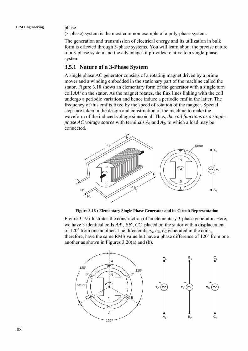
3.5.1 Nature of a 3-Phase System A single phase AC generator consists of a rotating magnet driven by a prime mover and a winding embedded in the stationary part of the machine called the stator. Figure 3.18 shows an elementary form of the generator with a single turn coil AA′ on the stator. As the magnet rotates, the flux lines linking with the coil undergo a periodic variation and hence induce a periodic emf in the latter. The frequency of this emf is fixed by the speed of rotation of the magnet. Special steps are taken in the design and construction of the machine to make the waveform of the induced voltage sinusoidal. Thus, the coil functions as a single-phase AC voltage source with terminals A1 and A2, to which a load may be connected.

N

S

A

A'

Stator

~

A1

A2

eA

+

–

N

Se A

2–+

A 2

e A

A 1+

–

e A

A

A'

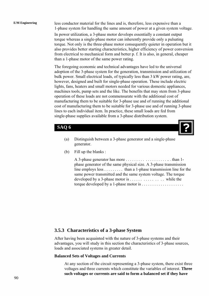
Figure 3.18 : Elementary Single Phase Generator and its Circuit Representation Figure 3.19 illustrates the construction of an elementary 3-phase generator. Here, we have 3 identical coils AA′, BB′, CC′ placed on the stator with a displacement of 120o from one another. The three emfs eA, eB, eB C generated in the coils, therefore, have the same RMS value but have a phase difference of 120 from one another as shown in Figures 3.20(a) and (b).

o

A'

A

C'B'

C B

N

S

Stator

120º120º

120º

~

A1

A2

eA

+

~

B1

B2

eB

+

~

C1

C2

eC

+

89

Figure 3.19 : Elementary 3-phase Generator and its Circuit Representation AC Circuits

0

eA eB eC

ωt83π2π4

3π2

3π

(a) Waveforms

EA

EB

EC

120º

120º

120º

(b) Phasors

Figure 3.20 : Voltages Produced in a 3-phase Generator

3-phase generator can, therefore, be viewed as a composite unit comprising 3-single-phase voltage sources with a fixed phase difference of 120o between any two of them. In practice, it is rare for a 3-phase generator to have all the six terminals brought out. The three coils are connected either in star or delta and only 3 or 4 terminals are brought out, as we shall see later.

A 3-phase system contains 3-phase sources besides 3-phase load impedances and feeder lines interconnecting them. The three individual sections which constitute a 3-phase source besides 3-phase arrangement are referred to as Phase A, Phase B, and Phase C respectively. Another common practice is to label them as R (red), Y (yellow) and B (blue) phases. We shall follow the former convention in our work. 3.5.2 Merits of a 3-Phase System Let us now look at the advantages provided by 3-phase systems relative to single-phase systems. A 3-phase AC generator utilises the available space on the stator more effectively than 1-phase generator and has 50% more kVA rating for the same physical size. All commercial power stations, therefore, employ 3-phase generators as they cost less than single-phase generators for the same kVA rating. The cost of electrical transmission and distribution lines used to carry bulk power from generating stations to receiving substations and distribute power from the substations to different load centres depends substantially on the volume of conducting material (usually aluminium) required for constructing these lines. It turns out that a 3-phase arrangement for transmission and distribution requires

90

less conductor material for the lines and is, therefore, less expensive than a 1-phase system for handling the same amount of power at a given system voltage.

E/M Engineering

In power utilization, a 3-phase motor develops essentially a constant output torque whereas a single-phase motor can inherently provide only a pulsating torque. Not only is the three-phase motor consequently quieter in operation but it also provides better starting characteristics, higher efficiency of power conversion from electrical to mechanical form and better p. f. It is also, in general, cheaper than a 1-phase motor of the same power rating.

The foregoing economic and technical advantages have led to the universal adoption of the 3-phase system for the generation, transmission and utilization of bulk power. Small electrical loads, of typically less than 3 kW power rating, are, however, designed and built for single-phase operation. These include electric lights, fans, heaters and small motors needed for various domestic appliances, machines tools, pump sets and the like. The benefits that may stem from 3-phase operation of these loads are not commensurate with the additional cost of manufacturing them to be suitable for 3-phase use and of running the additional cost of manufacturing them to be suitable for 3-phase use and of running 3-phase lines to each individual item. In practice, these small loads are fed from single-phase supplies available from a 3-phase distribution system.

SAQ 6

(a) Distinguish between a 3-phase generator and a single-phase generator.

(b) Fill up the blanks :

A 3-phase generator has more . . . . . . . . . . . . . . . . . . . .. . than 1-phase generator of the same physical size. A 3-phase transmission line employs less . . . . . . . . . than a 1-phase transmission line for the same power transmitted and the same system voltage. The torque developed by a 3-phase motor is . . . . . . . . . . . . . . . while the torque developed by a 1-phase motor is . . . . . . . . . . . . . . . . . . . .

3.5.3 Characteristics of a 3-phase System After having been acquainted with the nature of 3-phase systems and their advantages, you will study in this section the characteristics of 3-phase sources, loads and associated systems in greater detail.

Balanced Sets of Voltages and Currents At any section of the circuit representing a 3-phase system, there exist three voltages and three currents which constitute the variables of interest. Three such voltages or currents are said to form a balanced set if they have

91

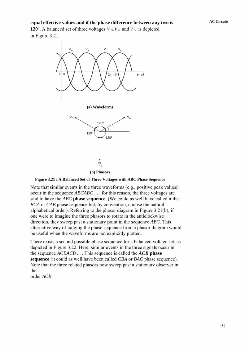
AC Circuitsequal effective values and if the phase difference between any two is

120o. A balanced set of three voltages CBA VVV and, is depicted in Figure 3.21.

0

VA VB VC

ωt2π − θ

VA

−θ

(a) Waveforms

VA

120º

120º

120º

VC

VB

θ

(b) Phasors

Figure 3.21 : A Balanced Set of Three Voltages with ABC Phase Sequence

Note that similar events in the three waveforms (e.g., positive peak values) occur in the sequence ABCABC . . . for this reason, the three voltages are said to have the ABC phase sequence. (We could as well have called it the BCA or CAB phase sequence but, by convention, choose the natural alphabetical order). Referring to the phasor diagram in Figure 3.21(b), if one were to imagine the three phasors to rotate in the anticlockwise direction, they sweep past a stationary point in the sequence ABC. This alternative way of judging the phase sequence from a phasor diagram would be useful when the waveforms are not explicitly plotted.

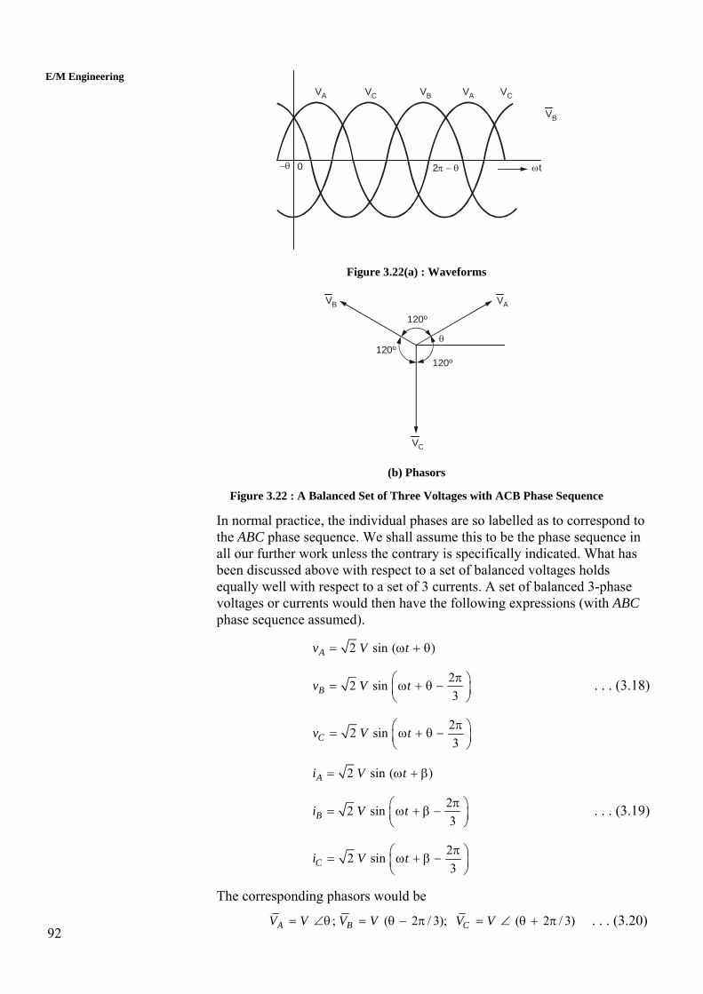
There exists a second possible phase sequence for a balanced voltage set, as depicted in Figure 3.22. Here, similar events in the three signals occur in the sequence ACBACB . . . This sequence is called the ACB phase sequence (it could as well have been called CBA or BAC phase sequence). Note that the three related phasors now sweep past a stationary observer in the order ACB.

92

0

VA VC VB

ωt2π − θ

VA

VB

−θ

VC

E/M Engineering

Figure 3.22(a) : Waveforms

VA

120º

120º

120º

VB

VC

θ

(b) Phasors

Figure 3.22 : A Balanced Set of Three Voltages with ACB Phase Sequence

In normal practice, the individual phases are so labelled as to correspond to the ABC phase sequence. We shall assume this to be the phase sequence in all our further work unless the contrary is specifically indicated. What has been discussed above with respect to a set of balanced voltages holds equally well with respect to a set of 3 currents. A set of balanced 3-phase voltages or currents would then have the following expressions (with ABC phase sequence assumed).

2 sin ( )Av V t= ω + θ

22 sin3Bv V t π⎛ ⎞= ω + θ −⎜ ⎟

⎝ ⎠ . . . (3.18)

22 sin3Cv V t π⎛ ⎞= ω + θ −⎜ ⎟

⎝ ⎠

2 sin (Ai V t )= ω + β

22 sin3Bi V t π⎛ ⎞= ω + β −⎜ ⎟

⎝ ⎠ . . . (3.19)

22 sin3Ci V t π⎛ ⎞= ω + β −⎜ ⎟

⎝ ⎠

The corresponding phasors would be

; ( 2 / 3); ( 2 / 3)A B CV V V V V V= ∠θ = θ − π = ∠ θ + π . . . (3.20)

93

AC Circuits ; ( 2 / 3); ( 2 / 3)A B CI I I I I I= ∠ β = β − π = ∠ β + π . . . (3.21)

The following properties of balanced voltages (or currents) are noteworthy :

With ABC phase sequence, vA leads vB by 120 , vB

oBB leads vC by 120o and vC

leads vA by 120o. With ACB phase sequence, vA leads vC by 120o, vC leads vB by 120 and vB

oBB leads vA by 120o.

If the set of voltages (or currents) is known to be balanced and the phase sequence is fixed, the data pertaining to one voltage or current would suffice to deduce the other two. For example, if it is known that

o30100 ∠=BV and that the phase sequence is ABC, it follows that o150100 ∠=AV and o90100 −∠=CV .

The sum of three balanced quantities is identically zero in time domain.

vA + vB + vB C = 0 . . . (3.22)

iA + iB + iB C = 0 . . . (3.23)

The above results can be proved through manipulation of the trigonometric expressions in Eqs. (3.18) and (3.19). They can also be verified by observing that the ordinates of the three pertinent waveforms like those in Figure 3.22(a) add up to zero at every instant of time.

The equivalent results in phasor domain are

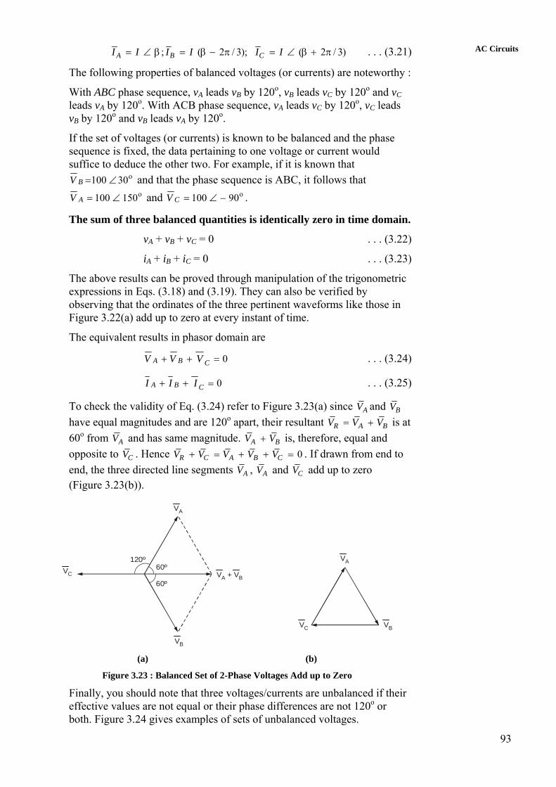
0=++ CBA VVV . . . (3.24)

0=++ CBA III . . . (3.25)

To check the validity of Eq. (3.24) refer to Figure 3.23(a) since AV and BV have equal magnitudes and are 120o apart, their resultant R AV V V= + B is at 60o from AV and has same magnitude. A BV V+ is, therefore, equal and opposite to CV . Hence 0R C A B CV V V V V+ = + + = . If drawn from end to end, the three directed line segments AV , AV and CV add up to zero (Figure 3.23(b)).

60º

60º

120ºVC

VB

VA + VB

VC VB

VA

VA

(a) (b)

Figure 3.23 : Balanced Set of 2-Phase Voltages Add up to Zero

Finally, you should note that three voltages/currents are unbalanced if their effective values are not equal or their phase differences are not 120o or both. Figure 3.24 gives examples of sets of unbalanced voltages.

94

120º120º

120º

VB

VA

VC

VB

VC

VA

VC

VB

VA

E/M Engineering

(a) (b) (c)

Figure 3.24 : Examples of Sets of Unbalanced Voltages

Example 3.7

At a certain section in a 3-phase circuit, o120 60BV = ∠ and o4 180CI = ∠ . If the voltages and currents are balanced and the phase

sequence is ABC, deduce AV , BV , AI and BI .

Solution With ABC sequence, BV leads CV by 120o. Thus,

o o120 180 ; 120 60A CV V= ∠ = ∠ −

CI leads AI by 120o and lags BI by 120o

o o4 60 ; 4 60A BI I⇒ = ∠ = ∠ − .

3.5.4 Star and Delta Connections You would recall that a 3-phase generator essentially consists of 3 single-phase sources, having output voltages say, eA, eB and eB C. A balanced 3-phase source is one in which these three voltages form a balanced set. All commercial 3-phase generators are built in this manner. The three single-phase sources are connected internally either in delta or in star as shown in Figure 3.25 and terminals brought out for connection to external loads.

Note the symmetrical way of connecting the three single-phase sources. In the delta connection, A2 is connected to BB1, B2 is connected to C1 and C2 is connected to A1. In the star connection, A2, B2 B and C2 are joined together. Such an orderly method of connections is needed to ensure the balanced condition of the voltages available between the terminals A, B and C of the 3-phase generator.

In the delta connection, the effective emf of the three series connected sources around the closed circuit is eA + eB + eB C. If the three voltages do not add up to zero there would be a large circulating current in the delta even with no load connected to terminals A, B, C and this is clearly an undesirable situation. However, for a balanced source this contingency does not arise as eA + eBB + eC = 0. It is this fact which makes the delta connection of a 3-phase source feasible.

95

AC Circuits

~

~ ~

C1

CB2 B1eB

– +

A2

eC–

+

+

–eA

C2 A1

A

~

CC1

B1

eC+

A2B2

A

B~ +

eB

A1

~ +eA

C2 ~

CC1

B1

eC+

A2B2

A

B~ +

eB

A1

~ +eA

C2

N

B

(a) (b) (c)

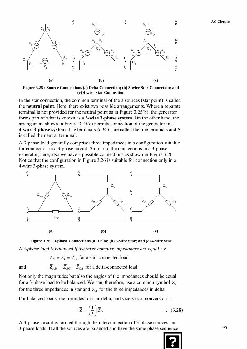
Figure 3.25 : Source Connections (a) Delta Connection; (b) 3-wire Star Connection; and (c) 4-wire Star Connection

In the star connection, the common terminal of the 3 sources (star point) is called the neutral point. Here, there exist two possible arrangements. Where a separate terminal is not provided for the neutral point as in Figure 3.25(b), the generator forms part of what is known as a 3-wire 3-phase system. On the other hand, the arrangement shown in Figure 3.25(c) permits connection of the generator in a 4-wire 3-phase system. The terminals A, B, C are called the line terminals and N is called the neutral terminal. A 3-phase load generally comprises three impedances in a configuration suitable for connection in a 3-phase circuit. Similar to the connections in a 3-phase generator, here, also we have 3 possible connections as shown in Figure 3.26. Notice that the configuration in Figure 3.26 is suitable for connection only in a 4-wire 3-phase system.

A

ZCA ZAB

ZBC

C

B

A

C

B

C

B

A

N

ZC ZB

ZA ZA

ZBZC

(a) (b) (c)

Figure 3.26 : 3-phase Connections (a) Delta; (b) 3-wire Star; and (c) 4-wire Star

A 3-phase load is balanced if the three complex impedances are equal, i.e.

A B CZ Z Z= = for a star-connected load

and AB BC CAZ Z Z= = for a delta-connected load

Not only the magnitudes but also the angles of the impedances should be equal for a 3-phase load to be balanced. We can, therefore, use a common symbol YZ for the three impedances in star and AZ for the three impedances in delta.

For balanced loads, the formulas for star-delta, and vice-versa, conversion is

13

YZ Z Δ⎛ ⎞= ⎜ ⎟⎝ ⎠

. . . (3.28)

A 3-phase circuit is formed through the interconnection of 3-phase sources and 3-phase loads. If all the sources are balanced and have the same phase sequence

96

and all the loads are also balanced, then the 3-phase circuit is said to be balanced. A characteristic of a balanced 3-phase circuit is that the voltages and currents at any arbitrary location are balanced. In our study, we shall be concerned only with balanced systems.

E/M Engineering

SAQ 7 (a) Fill u

The ________________________1 connection of sources/impedances is suitable either for 3-wire or for 4-wire three-phase systems but the ____________________2 connection of sources/impedances is suitable only for ________________________3 three-phase systems.

(b) State if the following assertions are true or false.

(i) Three impedances ,A BZ Z and CZ form a balanced 3-phase load if 0A B CZ Z Z+ + = .

(ii) The neutral point is not available in a 3-phase delta-connected source.

Example 3.8

A balanced 3-phase load is formed by three impedances of 60 + j90 ohms each, connected in delta. If this load is equivalent to a star-connected load having YZ in each leg of the star, calculate YZ .

Solution

1 1 (60 90) 20 303 3

YZ Z j jΔ= = + = + Ω

Relations between Line and Phase Quantities

In 3-phase circuits, one distinguishes between line voltages and currents on one hand and phase voltages and currents on the other. Phase quantities are the internal voltages or currents associated with the single phase sources constituting a 3-phase source or the three impedances constituting the 3-phase load. Line quantities, on the other hand, are those which can be measured at the 3-external terminals. These are the voltages between and the current in the external supply lines connected to the terminals.

Star Connection

The line and phase quantities for star connected balanced 3-phase system are shown in Figure 3.27.

97

~ ~

C

B

VL

~ VP

IL A

B

C

N N

A

VP VL

VL

VP

IP

IPIP

IL

IL

IL

VP

VPVP

VL

VL

VL

IP

IP IP

IL

IL

AC Circuits

(a) (b)

Figure 3.27

– VAN

– VBN VABVCNVCA

VAN

30º30º

VBC

– VCNVBN

(c)

Figure 3.27 : Phase and Line Quantities in a Star-connected (a) Source; (b) Load; and (c) Deduction of Line Voltages from Phase Voltages in a Balanced Star Configuration

A balanced star configuration has the following important characteristics : • Phase currents and line currents have the same effective value

(IL = IP). • Line voltages have 3 times the effective value of phase

voltage ( 3L PV V= ).

• The line voltages and phase voltages have the same phase sequence and the set of line voltages phasors is displaced by 30o from the set of phase voltage phasors.

Delta Connection Line and phase quantities for delta connected source and load are shown in Figure 3.28.

A

B

C

~

~ ~IP

VP VP

VP

VP

VP

VP

CIP IP

IL IL

IL IL

IP

IPIP

IL IL

VL VL

VL

VL VL

VL

+

–eA

A

B

(a) (b)

98

E/M Engineering

30º 30º

60º 60º

30º30º

30º30º

IC

IAIB

ICA

ICA

IAB

IBC

−IBC

−IAB

(c)

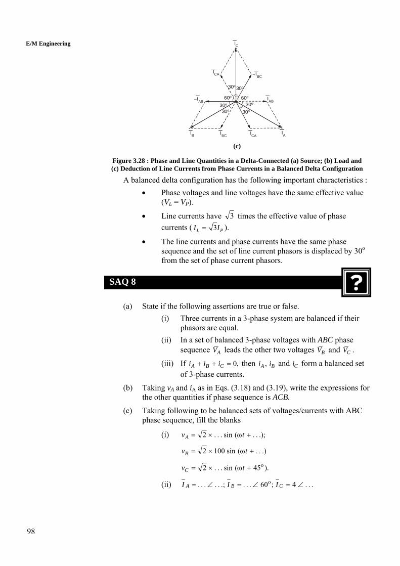
Figure 3.28 : Phase and Line Quantities in a Delta-Connected (a) Source; (b) Load and (c) Deduction of Line Currents from Phase Currents in a Balanced Delta Configuration

A balanced delta configuration has the following important characteristics : • Phase voltages and line voltages have the same effective value

(VL = VP).

• Line currents have 3 times the effective value of phase currents ( 3L PI I= ).

• The line currents and phase currents have the same phase sequence and the set of line current phasors is displaced by 30o from the set of phase current phasors.

SAQ 8

(a) State if the following assertions are true or false. (i) Three currents in a 3-phase system are balanced if their

phasors are equal. (ii) In a set of balanced 3-phase voltages with ABC phase

sequence AV leads the other two voltages BV and CV .

(iii) If ,0=++ CBA iii then , andA Bi i iC form a balanced set of 3-phase currents.

(b) Taking vA and iA as in Eqs. (3.18) and (3.19), write the expressions for the other quantities if phase sequence is ACB.

(c) Taking following to be balanced sets of voltages/currents with ABC phase sequence, fill the blanks

(i) .);..(sin...2 +ω×= tvA

.)..(sin1002 +ω×= tvB

).45(sin...2 o+ω×= tvC

(ii) ...4;60...;...... o ∠=∠=∠= CBA III

99

AC Circuits3.6 SUMMARY

In this unit, the main emphasis was on the study of single-phase AC circuits and the concepts of three phase systems.

Sinusoidal voltages and currents called AC voltages and currents play a key role in the theory and practice of electrical engineering. Here, you have learnt how to calculate response of R, L, C elements to sinusoidal excitation and also how to calculate power.

You have also been introduced to the basic features of a 3-phase voltages and currents.

In the next unit, the electrical machines and power distribution will be discussed.

3.7 ANSWERS TO SAQs

SAQ 1

(a) o100 sin ( 30 )t− ω +

o100 sin ( 150 )t= ω −

150o

100/ 2√

(b) o4 2 cos ( 30 )tω +

o4 2 cos ( 120 )t= ω +

120o

SAQ 2

(a) (i) leads

(i) 90

(ii) resistor

(iii) smaller

(b) 230 = (2π × 50) L × 1.1 ⇒ L = 0.666 H

Changed current = 1.435A2550

2301501.1 =××

Also, A435.1666.0502

150=

××π=

ω=

LVI

SAQ 3

(a) The statement is false. It is the ratio of phasors of v(t) and i(t), which is equal to the impedance.

(b) R-1, 1/jωL, jωC

SAQ 4

100

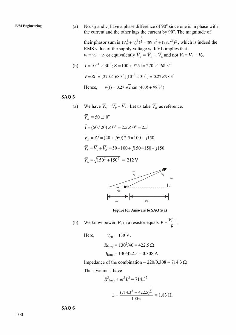
(a) No. vR and vc have a phase difference of 90o since one is in phase with the current and the other lags the current by 90o. The magnitude of

their phasor sum is 1 1

2 2 2 22( ) (89.8 178.7 )R cV V+ = +

E/M Engineering

2 , which is indeed the RMS value of the supply voltage vs. KVL implies that vs = vR + vc or equivalently CRS VVV += and not Vs = VR + Vc.

(b) oo jZI 3.68270251100;3010 3 ∠=+=∠= −

o 3 o[270 68.3 ][10 30 ] 0.27 98.3V ZI −= = ∠ ∠ = ∠ o

Hence, )3.98400(sin227.0)( o+= ttv

SAQ 5

(a) We have ZRS VVV += . Let us take RV as reference.

RV = 50 ∠ 0o

5.205.20)20/50( =∠=∠= ooI

1501005.2)6040( jjIZVZ +=+==

15015015010050 jjVVV ZRS +=++=+=

V212150150 22 =+=SV

VzVs

VR

50

50 100

Figure for Answers to SAQ 5(a)

(b) We know power, P, in a resistor equals R

VP2

eff= .

Here, . V130eff =V

Rlamp = 1302/40 = 422.5 Ω

Ilamp = 130/422.5 = 0.308 A

Impedance of the combination = 220/0.308 = 714.3 Ω

Thus, we must have

R2lamp + ω2 L2 = 714.32

π

−=

100)5.4223.714( 2

12

L = 1.83 H.

SAQ 6

101

AC Circuits(a) A single-phase generator has two terminals and produces a single

output voltage between the two terminals. A 3-phase generator is a composite unit comprising 3-single-phase generators, each generator producing a voltage which has fixed phase difference with the other two. The three 1-phase generators are connected internally in star or delta and the resulting 3-phase generator has 3 or 4 external terminals.

(b) (i) kVA rating

(ii) conductor material

(iii) constant

(iv) pulsating

SAQ 7

(a) Star1, Delta2, and 3-wire3

(b) (i) False

(ii) True

SAQ 8

(a) (i) False

(ii) False. CV leads AV by 120o (angle of lag/lead is limited to 180o).

(iii) False. The converse of the statement above Eq. (3.23) is not necessarily true. For example, iA, iB and iB C with iA = − iBB and iC = 0 do not form a balanced set.

(b) ⎟⎠⎞

⎜⎝⎛ π

+θ+ω=3

2sin2 tVvB

⎟⎠⎞

⎜⎝⎛ π

−θ+ω=3

2sin2 tVvC

⎟⎠⎞

⎜⎝⎛ π

+β+ω=3

2sin2 tIiB

⎟⎠⎞

⎜⎝⎛ π

−β+ω=3

2sin2 tIiB

(c) (i) 100, 285o, 165o, 100.

(ii) 4, 180o, 4, – 60o.