Appendix

A.1 Constructing a Minimum Spanning Tree

A.1.1 Prim’s Algorithm

Prim’s algorithm is a greedy algorithm to construct the minimal spanning tree of agraph. The algorithm was independently developed in 1930 by Jarník [1] and laterby Prim in 1957 [2]. Therefore the algorithm is sometimes called as Jarník algorithmas well. This greedy algorithm starts with one node in the ‘tree’ and iteratively stepby step adds the edge with the lowest cost to the tree. The formal algorithm is givenin Algorithm 14.

Algorithm 14 Prim’s algorithmGiven a non-empty connected weighted graph G = (V, E), where V yields the set of the verticesand E yields the set of the edges.

Step 1 Select a node (x ∈ V ) arbitrary from the vertices. This node will be the root in the tree.Set Vnew = {x}, Enew = {}.

Step 2 Choose the edge with the lowest cost from the set of the edges e(u, v) such that u ∈ Enewand v �∈ Enew . If there are multiple edges with the same weight connecting to the tree constructedso far, any of them may be selected. Set Enew = Enew ∪ {v} and Vnew = Vnew ∪ {e(u, v)}.

Step 3 If Vnew �= V go back to Step 2.

A.1.2 Kruskal’s Algorithm

Kruskal’s algorithm [3] is an another greedy algorithm to construct the minimalspanning tree. This algorithm starts with a forest (initially each node of the graphrepresents a tree) and iteratively adds the edge with the lowest cost to the forestconnecting trees such a way, that circles in the forest are not enabled. The detailedalgorithm is given in Algorithm 15.

Á. Vathy-Fogarassy and J. Abonyi, Graph-Based Clustering 93and Data Visualization Algorithms, SpringerBriefs in Computer Science,DOI: 10.1007/978-1-4471-5158-6, © János Abonyi 2013

94 Appendix

Algorithm 15 Kruskal’s algorithmGiven a non-empty connected weighted graph G = (V, E), where V yields the set of the verticesand E yields the set of the edges.

Step 1 Create a forest F in such a way that each vertex (V ) of the graph G denotes a separatetree. Let S = E .

Step 2 Select an edge e from S with the minimum weight. Set S = S − {e}.Step 3 If the selected edge e connects two separated trees, then add it to the forest.Step 4 If F is not yet a spanning tree and S �= {} go back to Step 2.

A.2 Solutions of the Shortest Path Problem

A.2.1 Dijkstra’s Algorithm

Dijkstra’s algorithm calculates the shortest path from a selected vertex to every othervertex in a weighted graph where the weights of the edges non-negative numbers.Similar to Prim’s and Kruskal’s algorithms it is a greedy algorithm, too. It starts froma selected node s and iteratively adds the closest node to a so far visited set of nodes.The whole algorithm is described in Algorithm 16.

At the end of the algorithm the improved tentative distances of the nodes yieldstheir distances to vertex s.

Algorithm 16 Dijkstra’s algorithmGiven a non-empty connected weighted graph G = (V, E), where V yields the set of the verticesand E yields the set of the edges. Let s ∈ V the initial vertex from which we want to determine theshortest distances to the other vertices.

Step 0 Initialization: Denote Pvisited the set of the nodes visited so far and Punvisi ted the set ofthe nodes unvisited so far. Let Pvisi ted = {s}, Punvisi ted = V −{s}. Yield the vcurrent the currentnode and set vcurrent = s. Assign a tentative distance to each node as follows: set it to 0 fornode s (dists = 0) and to infinity for all other nodes.

Step 1 Consider all unvisited direct topological neighbors of the current node, and calculate theirtentative distances to the initial vertex as follows:

dists,ei = dists,vcurrent + wvcurrent ,ei , (A.1)

where ei ∈ Punvisited is a direct topological neighbor of vcurrent , and wvcurrent ,ei yields the weightof the edge between nodes vcurrent and ei .If the recalculated distance for ei is less than the previously calculated distance for ei , thanrecord it as its new tentative distance to s.

Step 2 Mark the current vertex as visited by setting Pvisited = Pvisited ∪ {vcurrent}, and remove itfrom the unvisited set by setting Punvisited = Punvisited − {vcurrent}.

Step 3 If Punvisited = {} or if the smallest tentative distance among the nodes in the unvisited setis infinity then stop. Else select the node with the smallest tentative distance to s from the set ofthe unvisited nodes, set this node as the new current node and go back to Step 1.

Appendix 95

A.2.2 Floyd-Warshall Algorithm

Given a weighted graph G = (V, E). The Floyd-Warshall algorithm (or Floyd’salgorithm) computes the shortest path between all pairs of the vertices of G. Thealgorithm operates on a n×n matrix representing the costs of edges between vertices,where n is the number of the vertices in G (‖V ‖ = n). The elements of the matrixare initialized and step by step updated as it is described in Algorithm 17.

Algorithm 17 Floyd-Warshall algorithmGiven a weighted graph G = (V, E), where V yields the set of the vertices and E yields the setof the edges. Let n = ‖V ‖ the number of the vertices. Denote D the matrix with dimension n × nthat stores the lenghts of the paths between the vertices. After running the algorithm elements of Dwill contain the lengths of the shortest paths between all pairs of edges G.

Step 1 Initialization of matrix D: If there is an edge between vertex i (vi ∈ V ) and vertex j(vi ∈ V ) in the graph, the cost of this edge is placed in position (i, j) and ( j, i) of the matrix. Ifthere is no edge directly linking two vertices, an infinite (or a very large) value is placed in thepositions (i, j) and ( j, i) of the matrix. For all vi ∈ V, i = 1, 2, . . . , n the elements (i, i) of thematrix is set to zero.

Step 2 Recalculating the elements of D.for (k = 1; k <= n; k + +)

for (i = 1; i <= n; i + +)

for ( j = 1; j <= n; j + +)

if Di, j > (Di,k + Dk, j ) then set Di, j = Di,k + Dk, j

A.3 Hierarchical Clustering

Hierarchical clustering algorithms may be divided into two main groups: (i) agglom-erative methods and (ii) divisive methods. The agglomerative hierarchical methodsstart with N clusters, where each cluster contains only an object, and they recursivelymerge the two most similar groups into a single cluster. At the end of the process theobjects will form only a single cluster. The divisive hierarchical methods begin withall objects in a single cluster and perform splitting until all objects form a discretepartition.

All hierarchical clustering methods work on similarity or distance matrices. Theagglomerative algorithms merge step by step those clusters that are the most similarand the divisive methods split those clusters that are most dissimilar. The similarityor distance matrices are updated step by step trough the iteration process. Although,the similarity or dissimilarity matrices are generally obtained from the Euclidiandistances of pairs of objects, the pairwise similarities of the clusters are definable ona numerous other ways.

The agglomerative hierarchical methods utilize most commonly the followingapproaches to determine the distances between the clusters: (i) single linkage method,(ii) complete linkage method and (iii) average linkage method. The single linkage

96 Appendix

method [4] is also known as the nearest neighbor technique. Using this similaritymeasure the agglomerative hierarchical algorithms join together the two clusterswhose two closest members have the smallest distance. The single linkage clusteringmethods are also often utilized in the graph theoretical algorithms, however thesemethods suffer from the chaining effect [5]. The complete linkage methods [6] (alsoknown as the furthest neighbor methods) calculate the pairwise cluster similaritiesbased on the furthest elements of the clusters. These methods merge the two clus-ters with the smallest maximum pairwise distance in each step. Algorithms basedon complete linkage methods produce tightly bound or compact clusters [7]. Theaverage linkage methods [8] consider the distance between two clusters to be equalto the average distance from any member of one cluster to any member of the othercluster. These methods merge those clusters where this average distance is the mini-mal. Naturally, there are other methods to determine the merging condition, e.g. theWard method, in which the merging of two clusters is based on the size of an errorsum of squares criterion [9].

The divisive hierarchical methods are computationally demanding. If the numberof the objects to be clustered is N , there are 2N−1 − 1 possible divisions to formthe next stage of the clustering procedure. The division criterion may be based on asingle variable (monothetic divisive methods) or the split can also be decided by theuse of all the variables simultaneously (polythetic divisive methods).

The nested grouping of objects and the similarity levels are usually displayed ina dendrogram. The dendrogram is a tree-like diagram, in which the nodes representthe clusters and the lengths of the stems represent the distances of the clusters to bemerged or split. Figure A.1 shows a typical dendrogram representation. It can be seen,in the case of the application of an agglomerative hierarchical method, objects a andb will be merged first, then the objects c and d will coalesce into a group, followingthis, the algorithm merges the clusters containing the objects {e} and {c, d}. Finally,all objects would belong to a single cluster.

One of the main advantages of the hierarchical algorithms is that the number ofthe clusters need not be specified a priori. There are several possibilities to chose theproper result from the nested series of the clusters. On the one hand, it is possible tostop the running of a hierarchical algorithm when the distance between the nearest

Fig. A.1 Dendrogram

a b c d e0

1

2

3

4

5

Appendix 97

clusters exceeds a predetermined threshold, or on the other hand the dendrogramalso offers a useful tool in the selection of the optimal result. The shape of thedendrogram informally suggests the number of the clusters and hereby the optimalclustering result.

Hierarchical clustering approaches are in close ties with graph based clustering.One of the best-known graph-theoretic divisive clustering algorithm (Zahn’s algo-rithm [10]) is based on the construction of the minimal spanning tree. This algorithmstep by step eliminates the ‘inconsistent’ edges from the graph and hereby results ina series of subgraphs.

A.4 Visual Assessment of Cluster Tendency

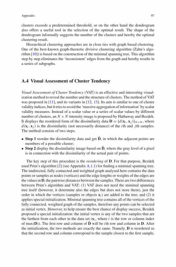
Visual Assessment of Cluster Tendency (VAT) is an effective and interesting visual-ization method to reveal the number and the structure of clusters. The method of VATwas proposed in [11], and its variants in [12, 13]. Its aim is similar to one of clustervalidity indices, but it tries to avoid the ‘massive aggregation of information’ by scalarvalidity measures. Instead of a scalar value or a series of scalar values by differentnumber of clusters, an N × N intensity image is proposed by Hathaway and Bezdek.It displays the reordered form of the dissimilarity data D = [d(xi , x j )]N×N , whered(xi , x j ) is the dissimilarity (not necessarily distance) of the i th and j th samples.The method consists of two steps.

• Step 1 reorder the dissimilarity data and get D, in which the adjacent points aremembers of a possible cluster;

• Step 2 display the dissimilarity image based on D, where the gray level of a pixelis in connection with the dissimilarity of the actual pair of points.

The key step of this procedure is the reordering of D. For that purpose, Bezdekused Prim’s algorithm [2] (see Appendix A.1.1) for finding a minimal spanning tree.The undirected, fully connected and weighted graph analysed here contains the datapoints or samples as nodes (vertices) and the edge lengths or weights of the edges arethe values in D, the pairwise distances between the samples. There are two differencesbetween Prim’s algorithm and VAT: (1) VAT does not need the minimal spanningtree itself (however, it determine also the edges but does not store them), just theorder in which the vertices (samples or objects xi ) are added to the tree; and (2) itapplies special initialization. Minimal spanning tree contains all of the vertices of thefully connected, weighted graph of the samples, therefore any points can be selectedas initial vertex. However, to help ensure the best chance of display success, Bezdekproposed a special initialization: the initial vertex is any of the two samples that arethe farthest from each other in the data set (xi , where i is the row or column indexof max(D)). The first row and column of D will be i th row and column in D. Afterthe initialization, the two methods are exactly the same. Namely, D is reordered sothat the second row and column correspond to the sample closest to the first sample,

98 Appendix

the third row and column correspond to the sample closest either one of the first twosamples, and so on.

This procedure is similar to the single-linkage algorithm that corresponds to theKruskal’s minimal spanning tree algorithm [3] (see Appendix A.1.2) and is basicallythe greedy approach to find a minimal spanning tree. By hierarchical clusteringalgorithms (such as single-linkage, complete-linkage or average-linkage methods),the results are displayed as a dendrogram, which is a nested structure of clusters.(Hierarchical clustering methods are not described here, the interested reader canrefer e.g. [8]). Bezdek et al. followed another way and they displayed the results asan intensity image I (D) with the size of N × N . The approach was presented in [13]as follows. Let G = {gm, . . . , gM } be the set of gray levels used for image displays.In the following, G = {0, . . . , 255}, so gm = 0 (black) and gM = 255 (white).Calculate

(I (D))i, j = Di, j

(gM

max(D)

). (A.2)

Convert (I (D))i, j to its nearest integer. These values will be the intensity displayedfor pixel (i, j) of I (D). In this form of display, ‘white’ corresponds to the maximaldistance between the data (and always will be two white pixels), and the darker thepixel the closer the two data are. (For large data sets, the image can easily exceedthe resolution of the display. To solve that problem, Huband, Bezdek and Hathawayhave been proposed variations of VAT [13]). This image contains information aboutcluster tendency. Dark blocks along the diagonal indicate possible clusters, and ifthe image exhibits many variations in gray levels with faint of indistinct dark blocksalong the diagonal, then the data set “[. . .] does not contain distinct clusters; or theclustering scheme implicitly imbedded in the reordering strategy fails to detect theclusters (there are cluster types for which single-linkage fails famously [. . .]).”

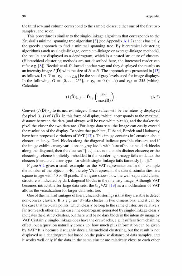
Figure A.2 gives a small example for the VAT representation. In this examplethe number of the objects is 40, thereby VAT represents the data dissimilarities in asquare image with 40 × 40 pixels. The figure shows how the well-separated clusterstructure is indicated by dark diagonal blocks in the intensity image. Although VATbecomes intractable for large data sets, the bigVAT [13] as a modification of VATallows the visualization for larger data sets, too.

One of the main advantages of hierarchical clusterings is that they are able to detectnon-convex clusters. It is e.g. an ‘S’-like cluster in two dimensions; and it can bethe case that two data points, which clearly belong to the same cluster, are relativelyfar from each other. In this case, the dendrogram generated by single-linkage clearlyindicates the distinct clusters, but there will be no dark block in the intensity image byVAT. Certainly, single-linkage does have the drawbacks, e.g. it suffers from chainingeffect, but a question naturally comes up: how much plus information can be givenby VAT? It is because it roughly does a hierarchical clustering, but the result is notdisplayed as a dendrogram but based on the pairwise distance of data samples, andit works well only if the data in the same cluster are relatively close to each other

Appendix 99

0 0.2 0.4 0.6 0.8 10

0.1

0.2

0.3

0.4

0.5

0.6

0.7

0.8

0.9

1

5 10 15 20 25 30 35 400

5

10

15

20

25

30

35

40

(a) (b)

Fig. A.2 The VAT representation. a The original data set. b VAT

0

0.02

0.04

0.06

0.08

0.1

0.12

0.14

0.16

Lev

el

Single Linkage on the Original Data

Fig. A.3 Result of the (left) single-linkage algorithm and (right) VAT on synthetic data

based on the original distance norm. (This problem arises not only by clusters withnon-convex shape, but very elongated ellipsoids as well.) Therefore, one advantageof hierarchical clustering is lost.

In Fig. A.3 results of the single-linkage algorithm and VAT can be seen on thesynthetic data. The clusters are well-separated but non-convex, and single-linkageclearly identifies them as can be seen from the dendrogram. However, the VAT imageis not as clear as the dendrogram in this case because there are data in the ‘S’ shapedcluster that are far from each other based on the Euclidean distance norm (see thetop and left corner of the image).

100 Appendix

A.5 Gath-Geva Clustering Algorithm

Fuzzy clustering methods assign degrees of membership in several clusters to eachinput pattern. The resulted fuzzy partition matrix (U) describes the relationship ofthe objects and the clusters. The fuzzy partition matrix U = [μi,k] is a c × N matrix,where μi,k denotes the degree of the membership of xk in cluster Ci , so the i-throw of U contains values of the membership function of the i-th fuzzy subset of X.Conditions of the fuzzy partition matrix are given:

μi,k ∈ [0, 1], 1 ≤ i ≤ c, 1 ≤ k ≤ N , (A.3)c∑

i=1

μi,k = 1, 1 ≤ k ≤ N , (A.4)

0 <

N∑k=1

μi,k < N , 1 ≤ i ≤ c. (A.5)

The meaning of the relations written above is that the degree of the membershipis a real number in [0,1] (A.3); the sum of the membership values of an object isexactly one (A.4); each cluster must contain at least one object with membershipvalue larger than zero, and the sum of the degrees of the membership values can notexceed the number of elements considered (A.5).

Based on the previous statements the fuzzy partitioning space can be formulated asfollows: Let X = {x1, x2, . . . , xN } be a finite set of the observed data, let 2 ≤ c ≤ Nbe an integer. The fuzzy partitioning space for X is the set

M f c ={

U ∈ Rc×n|μi,k ∈ [0, 1] ,∀i, k;

c∑i=1

μi,k = 1,∀k; 0 <

N∑k=1

μi,k < N ,∀i

}

(A.6)

A common limitation of partitional clustering algorithms based on a fixed distancenorm, like k-means or fuzzy c-means clustering is, that they induce a fixed topologicalstructure and force the objective function to prefer clusters of spherical shape even if itis not present. Generally, different cluster shapes (orientations, volumes) are requiredfor the different clusters, but there is no guideline as to how to choose them a priori.

Mixture-resolving methods (e.g. Gustafson-Kessel, Gath-Geva) assume that theobjects to be clustered are drawn from one of several distributions (usually Gaussian),and hereby different clusters may form different shapes and sizes. The main task andat the same time the main difficulty of these methods is to estimate the parametersof all these distributions. These algorithms apply several norm-inducing matrices toestimate the data covariance in each cluster. Most of the mixture-resolving methodsassume that the individual components of the mixture density are Gaussians, andin this case the parameters of the individual Gaussians are to be estimated by theprocedure.

Appendix 101

Traditional approaches to this problem involve obtaining (iteratively) a maximumlikelihood estimate of the parameter vectors of the component densities [8]. Morerecently, the Expectation Maximization (EM) algorithm (a general purpose maxi-mum likelihood algorithm [14] for missing-data problems) has been applied to theproblem of parameter estimation. The Gustafson-Kessel (GK) [15] and the Gaussianmixture based fuzzy maximum likelihood estimation (Gath-Geva algorithm (GG)[16]) algorithms are also based on an adaptive distance norm, and they are ableto estimate the underlying distribution of the objects. Hereby, these algorithms areable to disclose clusters with different orientation and volume. The Gath-Geva (GG)algorithm can be seen as a further development of the Gustafson-Kessel algorithm.In Gath-Geva algorithm the cluster sizes are not restricted like in Gustafson-Kesselmethod, and the cluster densities are also taken into consideration. Unfortunately,the GG algorithm is very sensitive to initialization, hence often it can not be directlyapplied to the data.

As we have seen, the exploration of the shapes of the clusters is an essentialtask. The shape of the clusters can be determined by the distance norm. The typicaldistance norm between the object xk and the cluster center vi is represented as:

D2i,k = ‖xk − vi‖2

A = (xk − vi )T A(xk − vi ), (A.7)

where A is a symmetric and positive definite matrix. Different distance norms canbe induced by the choice of the matrix A. The Euclidean distance arises with thechoice of A = I where I is an identity matrix. The Mahalanobis normis inducedwhen A = F−1 where F is the covariance matrix of the objects. It can be seenthat both the Euclidean and the Mahalanobis distances are based on fixed distancenorms. The Euclidean norm based methods find only hyperspherical clusters, and theMahalanobis norm based methods find only hyperellipsoidal ones (see Fig. A.4) even

x1x1

Euclidean norm Mahalanobis norm

x2x2

Fig. A.4 Different distance norms in fuzzy clustering

102 Appendix

if those shapes of clusters are not present in the data set. The norm-inducing matrixof the cluster prototypes can be adapted by using estimates of the data covariance,and can be used to estimate the statistical dependence of the data in each cluster.The Gustafson-Kessel algorithm (GK) [15] and the Gaussian mixture based fuzzymaximum likelihood estimation algorithm (Gath-Geva algorithm (GG) [16]) arebased on such an adaptive distance measure, they can adapt the distance norm tothe underlying distribution of the data which is reflected in the different sizes of theclusters, hence they are able to detect clusters with different orientation and volume.

Algorithm 18 Gath-Geva algorithmGiven a set of data X, specify the number of the clusters c, choose a weighting exponent m > 1and a termination tolerance ε > 0. Initialize the partition matrix U(0).

Repeat for t = 1, 2, . . .

Step 1 Calculate the cluster centers: v(t)i =

N∑k=1

(μ(t−1)i,k )m xk

N∑k=1

(μ(t−1)i,k )m

, 1 ≤ i ≤ c

Step 2 Compute the distance measure D2i,k . The distance to the prototype is calculated based

on the fuzzy covariance matrices of the cluster

F(t)i =

N∑k=1

(μ(t−1)i,k )m

(xk − v(t)

i

) (xk − v(t)

i

)T

N∑k=1

(μ(t−1)i,k )m

, 1 ≤ i ≤ c (A.8)

The distance function is chosen as

D2i,k(xk , vi ) = (2π)

(N2

)√det (Fi )

αiexp

(1

2

(xk − v(t)

i

)TF−1

i

(xk − v(t)

i

))(A.9)

with the a priori probability αi = 1N

N∑k=1

μi,k

Step 3 Update the partition matrix

μ(t)i,k = 1∑c

j=1

(Di,k (xk , vi ) /D j,k

(xk , v j

))2/(m−1), 1 ≤ i ≤ c, 1 ≤ k ≤ N (A.10)

Until ||U(t) − U(t−1)|| < ε.

Appendix 103

A.6 Data Sets

A.6.1 Iris Data Set

The Iris data set [17] (http://www.ics.uci.edu) contains measurements on three class-es of iris flowers. The data set was made by measurements of sepal length and widthand petal length and width for a collection of 150 irises. The analysed data setcontains 50 samples from each class of iris flowers (Iris setosa, Iris versicolor andIris virginica). The problem is to distinguish the three different types of the iris flower.Iris setosa is easily distinguishable from the other two types, but Iris versicolor andIris virginica are very similar to each other. This data set has been analysed manytimes to illustrate various clustering methods.

A.6.2 Semeion Data Set

The semeion data set contains 1593 handwritten digits from around 80 persons. Eachperson wrote on a paper all the digits from 0 to 9, twice. First time in the normal wayas accurate as they can and the second time in a fast way. The digits were scanned andstretched in a rectangular box including 16 × 16 cells in a grey scale of 256 values.Then each pixel of each image was scaled into a boolean value using a fixed threshold.As a result the data set contains 1593 sample digits and each digit is characterisedwith 256 boolean variables. The data set is available form the UCI Machine LearningRepository [18]. The data set in the UCI Machine Learning Repository contains 266attributes for each sample digit, where the last 10 digits describe the classificationsof the digits.

A.6.3 Wine Data Set

The Wine database (http://www.ics.uci.edu) consists of the chemical analysis of178 wines from three different cultivars in the same Italian region. Each wine ischaracterised by 13 attributes, and there are 3 classes distinguished.

A.6.4 Wisconsin Breast Cancer Data Set

The Wisconsin breast cancer database (http://www.ics.uci.edu) is a well known diag-nostic data set for breast cancer compiled by Dr William H. Wolberg, University ofWisconsin Hospitals [19]. This data set contains 9 attributes and class labels for the

104 Appendix

Fig. A.5 Swiss roll data set

0 5 10 15 20 25 010

20300

5

10

15

20

25

30

683 instances (16 records with missing values were deleted) of which 444 are benignand 239 are malignant.

A.6.5 Swiss Roll Data Set

The Swiss roll data set is a 3-dimensional data set with a 2-dimensional nonlinearlyembedded manifold. The 3-dimensional visualization of the Swiss roll data set isshown in Fig. A.5.

A.6.6 S Curve Data Set

The S curve data set is a 3-dimensional synthetic data set, in which data points areplaced on a 3-dimensional ‘S’ curve. The 3-dimensional visualization of the S curvedata set is shown in Fig. A.6.

A.6.7 The Synthetic ‘Boxlinecircle’ Data Set

The synthetic data set ‘boxlinecircle’ was made by the authors of the book. The dataset contains 7100 sample data placed in a cube, in a refracted line and in a circle. Asthis data set contains shapes with different dimensions, it is useful to demonstratethe various selected methods. Data points placed in the cube contain random errors(noise), too. In Fig. A.7 data points are yield with blue points and the borders of thepoints are illustrated with red lines.

Appendix 105

−1 −0.5 0 0.5 1 02

46−1

−0.5

0

0.5

1

1.5

2

2.5

3

Fig. A.6 S curve data set

−5 0 5 10 15 20 −50

5

−5

0

5

Fig. A.7 ‘Boxlinecircle’ data set

A.6.8 Variety Data Set

The Variety data set is a synthetic data set which contains 100 2-dimensional dataobjects. 99 objects are partitioned in 3 clusters with different sizes (22, 26 and 51objects), shapes and densities, and it also contains an outlier. Figure A.8 shows thenormalized data set.

106 Appendix

0 0.2 0.4 0.6 0.8 10

0.1

0.2

0.3

0.4

0.5

0.6

0.7

0.8

0.9

1

Fig. A.8 Variety data set

Fig. A.9 ChainLink data set

0 0.2 0.4 0.6 0.8 10

0.1

0.2

0.3

0.4

0.5

0.6

0.7

0.8

0.9

1

A.6.9 ChainLink Data Set

The ChainLink data set is a synthetic data set which contains 75 2-dimensional dataobjects. The objects can be partitioned into 3 clusters and a chain link which connects2 clusters. Hence linkage based methods often suffer from the chaining effect, thisexample tends to illustrate this problem. Figure A.9 shows the normalised data set.

Appendix 107

Fig. A.10 Curves data set

0 0.2 0.4 0.6 0.8 10

0.1

0.2

0.3

0.4

0.5

0.6

0.7

0.8

0.9

1

A.6.10 Curves Data Set

The Curves data set is a synthetic data set which contains 267 2-dimensional dataobjects. The objects can be partitioned into 4 clusters. What makes this data set inter-esting is that the objects form clusters with arbitrary shapes and sizes, furthermorethese clusters lie very near to each other. Figure A.10 shows the normalised data set.

References

1. Jarník, V.: O jistém problému minimálním [About a certain minimal problem]. Práce MoravskéPrírodovedecké Spolecnosti 6, 57–63 (1930)

2. Prim, R.C.: Shortest connection networks and some generalizations. In. Bell System TechnicalJournal 36, 1389–1401 (1957)

3. Kruskal, J.B: On the Shortest Spanning Subtree of a Graph and the Traveling Salesman Problem.In: Proceedings of the American Mathematical Society 7, No. 1, 48–50 (1956).

4. Sneath, P.H.A.: Sokal . Numerical taxonomy. Freeman, R.R. (1973)5. Nagy, G.: State of the art in pattern recognition. Proceedings of the IEEE 56(5), 836–862 (1968)6. King, B.: Step-wise clustering procedures. Journal of the American Statistical Association 69,

86–101 (1967)7. Baeza-Yates, R.A.: Introduction to data structures and algorithms related to information

retrieval. In Frakes, W.B., Baeza-Yates, R.A. (eds): Information Retrieval: Data Structuresand Algorithms, Prentice-Hall, 13–27 (1972).

8. Jain, A., Dubes, R.: Algorithms for Clustering Data. Prentice-Hall (1988).9. Ward, J.H.: Hierarchical grouping to optimize an objective function. Journal of the American

Statistical Association 58, 236–244 (1963)10. Zahn, C.T.: Graph-theoretical methods for detecting and describing gestalt clusters. IEEE

Transaction on Computers C20, 68–86 (1971)11. Bezdek, J.C., Hathaway, R.J.: VAT: A Tool for Visual Assessment of (Cluster) Tendency. IJCNN

2002, 2225–2230 (2002)

108 Appendix

12. Huband, J., Bezdek, J., Hathaway, R.: Revised Visual Assessment of (Cluster) Tendency(reVAT). Proceedings of the North American Fuzzy Information Processing Society (NAFIPS),101–104 (2004).

13. Huband, J., Bezdek, J., Hathaway, R.: bigVAT: Visual assessment of cluster tendency for largedata sets. Pattern Recognition 38(11), 1875–1886 (2005)

14. Dempster, A.P., Laird, N.M., Rubin, D.B.: Maximum likelihood from incomplete data via theEM algorithm. Journal of the Royal Statistical Society, Series B (Methodological) 39, 1–38(1977)

15. Gustafson, D.E., Kessel, W.C.: Fuzzy clustering with fuzzy covariance matrix. Proceedings ofthe IEEE CDC, 761–766 (1979).

16. Gath, I., Geva, A.B.: Unsupervised Optimal Fuzzy Clustering. IEEE Transactions on PatternAnalysis and Machine Intelligence 11, 773–781 (1989)

17. Fisher, R.A.: The Use of Multiple Measurements in Taxonomic Problems. Annals of Eugenics7, 179–188 (1936)

18. UC Irvine Machine Learning Repository www.ics.uci.edu/ mlearn/ Cited 15 Oct 2012.19. Mangasarian, O.L., Wolberg, W.H.: Cancer diagnosis via linear programming. Society for

Industrial and Applied Mathematics News 23(5), 1–18 (1990)

Index

Symbole-neighbouring, 2, 44

AAgglomerative hierarchical methods, 95Average linkage, 96

CCircle, 2Clustering

hierarchical, 95Codebook, 3Codebook vectors, 3Complete linkage, 96Continuous projection, 48Curvilinear component analysis, 65

DDelaunay triangulation, 4, 17Dendrogram, 96Dijkstra’s algorithm, 2, 94Dimensionality reduction, 44

linear, 45nonlinear, 45

Distance norm, 101Divisive hierarchical methods, 95Dunn’s index, 20Dynamic topology representing

network, 11

EEuclidean distance, 101

FFeature extraction, 44Feature selection, 44Floyd-Warshall algorithm, 95Forest, 1Fukuyama-Sugeno clustering

measure, 21Fuzzy hyper volume, 22Fuzzy neighbourhood similarity

measure, 31Fuzzy partition matrix, 100

GGabriel graph, 17Gath-Geva algorithm, 100, 102Geodesic distance, 2Geodesic nonlinear projection neural gas, 68Graph, 1

complete, 1connected, 1directed, 1disconnected, 1edge of graph, 1finite, 1node of graph, 1path in the graph, 2undirected, 1weighted, 1

Growing neural gas, 7Gustafson-Kessel algorithm, 100

HHybrid Minimal Spanning Tree—Gath-Geva

algorithm, 22

Á. Vathy-Fogarassy and J. Abonyi, Graph-Based Clusteringand Data Visualization Algorithms, SpringerBriefs in Computer Science,DOI: 10.1007/978-1-4471-5158-6, � János Abonyi 2013

109

IInconsistent edge, 18, 97Incremental grid growing, 59Independent component analysis, 45Isomap, 45, 62Isotop, 64

JJarvis-Patrick clustering, 18, 30

Kk-means algorithm, 3k-neighbouring, 2, 44knn graph, 2, 30Kruskal’s algorithm, 2, 18, 93, 98

LLBG algorithm, 4Locality preserving projections, 55

MMahalanobis distance, 101MDS stress function, 47Minimal spanning tree, 2, 17, 18Multidimensional scaling, 33, 52

metric, 52non-metric, 53

NNeighborhood, 1Neural gas algorithm, 5

OOnline visualisation neural gas, 67

PPartition index, 20Prim’s algorithm, 2, 18, 93Principal component analysis, 45, 49

RRelative neighbourhood graph, 17Residual variance, 47

SSammon mapping, 44, 45, 51Sammon stress function, 47Self-organizing Map, 45, 57Separation index, 20Single linkage, 96Spanning tree, 2

minimal, 2

TTopographic error, 48Topographic product, 48Topology representing network, 9Topology representing network map, 71Total fuzzy hyper volume, 22Transitive fuzzy neighbourhood similarity

measure, 32Tree, 1Trustworthy projection, 48

VVector quantization, 2Visual assessment of cluster tendency, 33, 97Visualisation, 43Voronoi diagram, 4

WWeighted incremental neural network, 13

ZZahn’s algorithm, 17, 18, 97

110 Index