a walk through bildverarbeitung ws 2010/11
TRANSCRIPT

1!
1!
A Walk through "Bildverarbeitung WS 2010/11"!
2!
Definition of Image Understanding!
Image understanding is the task-oriented reconstruction and interpretation of a scene by means of images !
scene: !section of the real world!!stationary (3D) or moving (4D)!
image: !view of a scene!!projection, density image (2D)!!depth image (2 1/2D)!!image sequence (3D)!
reconstruction !computer-internal scene description!and interpretation: !quantitative + qualitative + symbolic!
task-oriented: !for a purpose, to fulfill a particular task!!context-dependent, supporting actions of an agent!

2!
3!
Technical Colour Models!RGB colour model!
R!
G!
B!
magenta!cyan!
yellow!Typical discretization:!8 bits per colour dimension!=> 16,77,216 colours!
CMY colour model!
C !1 !R!M = !1 - !G!Y !1 !B!
HSI colour model!
Hue:!H = !Q !if B ≤ G!
!360 - Q !if B > G!!
! 1/2 [(R-G) + (R-B)]!Q = cos-1!
! [(R-G)2 + (R-B)(G-B)]1/2!
!Saturation:!
! 3!S = 1 - ! ! [min (R, G, B)]!
!(R + G + B)!!!Intensity:!I = 1/3 (R + G + B)!
4!
Sampling Theorem!
Shannon´s Sampling Theorem:!
A bandlimited function with bandwidth W can be exactly reconstructed from equally spaced samples, if the sampling distance is not larger than !1
2W
bandwidth = largest frequency contained in signal!(=> Fourier decomposition of a signal)!!Analogous theorem holds for 2D signals with limited spatial frequencies Wx and Wy!

3!
5!
Perspective Projection Geometry!
Projective geometry relates the coordinates of a point in a scene to the coordinates of its projection onto an image plane.!
Perspective projection is an adequate model for most cameras.!
•!
•!•!
x!y!
xp!
yp!
zp = f!
v = !x!!y!!z!
image plane!
optical center!
x f! z!xp =!
y f! z!yp=!
scene point!image point!
Projection equations:!
focal !distance f!
z = optical axis!
Vp = !xp!!yp!!zp!
6!
Connectivity in Digital Images!
Connectivity is an important property of subsets of pixels. It is based on adjacency (or neighbourhood):!
Pixels are 4-neighbours if their distance is D4 = 1!
Pixels are 8-neighbours if their distance is D8 = 1!
A path from pixel P to pixel Q is a sequence of pixels beginning at Q and ending at P, where consecutive pixels are neighbours.!
In a set of pixels, two pixels P and Q are connected, if there is a path between P and Q with pixels belonging to the set.!
A region is a set of pixels where each pair of pixels is connected.!
all 4-neighbours of center pixel!
all 8-neighbours of center pixel!

4!
7!
Principle of Greyvalue Interpolation!
•! •!•! •!
•! •!
•!•!
•!•!•!
•!
•!•!•! •!Greyvalue interpolation = computation of
unknown greyvalues at locations (u´v´) from known greyvalues at locations (x´y´)!
Two ways of viewing interpolation in the context of geometric transformations:!
A !Greyvalues at grid locations (x y) in old image are placed at corresponding locations (x´y´) in new image: g(x´y´) = g(T(x y))!!=> interpolation in new image!
B !Grid locations (u´v´) in new image are transformed into corresponding locations (u v) in old image: g(u v) = g(T-1(u´v´))!!=> interpolation in old image!
We will take view B: !Compute greyvalues between grid from greyvalues at grid locations.!
8!
Global Image Properties!
Global image properties refer to an image as a whole rather than components. Computation of global image properties is often required for image enhancement, preceding image analysis.!We treat!
!• empirical mean and variance!!• histograms!
!• projections!!• cross-sections!!• frequency spectrum!

5!
9!
Median Filter!Median of a distribution P(x): xm such that P(x < xm) = 1/2!!Median Filter:!ˆ g ij = max a with gk !D and | {gk < a}|< |D|
2
1. Sort pixels in D according to greyvalue!2. Choose greyvalue in middle position!
Example:! 11! 14! 15!
13! 12! 25!
15! 19! 26!
11!12!13!14!15!15!19!25!26!
greyvalue of center pixel of region is set to 15!
Median Filter reduces influence of outliers in either direction!!
10!
Discrete Fourier Transform (DFT)!
Guv =1
MN gmn
n=0
N!1
"m=0
M!1
" e!2#i( mu
M+nv
N)
gmn = Guvv=0
N!1
"u=0
M !1
" e2#i( mu
M+nv
N)
Transform is based on periodicity assumption!
Discrete Fourier Transform:! Inverse Discrete Fourier Transform:!
=> !periodic continuation may !cause boundary effects !
for u = 0 ... M-1, v = 0 ... N-1! for m = 0 ... M-1, n = 0 ... N-1!
Notation for computing the Fourier Transform:!Guv = F{ gmn }!
gmn = F-1{ Guv }!
Computes image representation as a sum of sinusoidals.!

6!
11!
Filtering in the Frequency Domain!A filter transforms a signal by modifying its spectrum.!
!G(u, v) = F(u, v) H(u, v)!
F !Fourier transform of the signal!H !frequency transfer function of the filter!G !modified Fourier transform of signal !
• !low-pass filter !low frequencies pass, high frequencies are ! ! !attenuated or removed!
• !high-pass filter !high frequencies pass, low frequencies are ! ! !attenuated or removed!
• !band-pass filter !frequencies within a frequency band pass, ! ! !other frequencies below or above are !! ! !attenuated or removed!
Often (but not always) the noise part of an image is high-frequency and the signal part is low-frequency. Low-pass filtering then improves the signal-to-noise ratio.!
12!
Convolution Using the FFT!
Convolution in the spatial domain may be performed more efficiently using the FFT.!
! g ij = gmnn=0
N -1
"m= 0
M#1
" hi#m,j#n (MN)2 operations needed!
Using the FFT and filtering in the frequency domain:!
gmn ! !Guv ! !Guv´ ! !gmn´!FFT! Huv! FFT-1!
MN log(MN) ! MN ! !MN log(MN) !# of operations!
Example with M = N = 512:!• !straight convolution needs ~ 1010 operations!• !convolution using the FFT needs ~107 operations!

7!
13!
Illustration of Minimum-loss Dimension Reduction!
Using the Karhunen-Loève transform data compression is achieved by !• !changing (rotating) the coordinate system!• !omitting the least informative dimension(s) in the new coodinate system!
Example:!
x1!
x2!
•! •!•!•!
•! •! •!•! •!
•!•!•!
•!
•!•!
x1!
x2!
•!•!•! •!•!•!•!•!•!•!•!•!•!
•!•!
y1!y2!
•! •!•!•!•! •!
•!
•!•!
•!
•! •! •!•! •! y1!
y2!
•!•!•! •!•!•!•!•!•!•!•!•!•! •!•! y1!
14!
Principle of Baseline JPEG!
FDCT! Quantizer! Entropy Encoder!
Encoder!
table!specifications!
table!specifications!
8 x 8 blocks!
source image data!
compressed image data!
(Source: Gibson et al., Digital Compression for Multimedia, Morgan Kaufmann 98)!
• !transform RGB into YUV coding, subsample color information!• !partition image into 8 x 8 blocks, left-to-right, top-to-bottom!• !compute Discrete Cosine Transform (DCT) of each block!• !quantize coefficients according to psychovisual quantization tables!• !order DCT coefficients in zigzag order!• !perform runlength coding of bitstream of all coefficients of a block!• !perform Huffman coding for symbols formed by bit patterns of a block !

8!
15!
Segmentation!
Segmenting the image into image elements which may correspond to meaningful scene elements!
high-level interpretations!
objects!
scene elements!
image elements!
raw images!
Typical results of first segmentation steps!
Example:!Partitioning an image into regions which may correspond to objects!
16!
Representing Regions!A region is a maximal 4- (or 8-) connected set of pixels. !
Methods for digital region representation:!• !grid occupancy!!- !labelling!!- !run-length coding!!- !quadtree coding!!- !cell sets!
• !boundary description!!- !chain code!!- !straight-line segments, polygons!!- !higher-order polynomials!
Note that discretizations of an analog region are not shift or rotation invariant:!
•! •! •! •!•! •! •! •!•! •! •! •!•! •! •! •!
•! •! •! •!•! •! •! •!•! •! •! •!•! •! •! •!
•! •! •! •!•! •! •! •!•! •! •! •!•! •! •! •!

9!
17!
Chain Code!Chain code represents boundaries by "chaining" direction arrows between successive boundary elements. !
0!1!
2!3!4!
5!6! 7!
Arbitrary choice of starting point, chain code can be represented e.g. by!{456671123}!Normalization by circular shift until the smallest integer is obtained:!{112345667}!
Chain code for 8-connectivity:!
0!
1!
2!
3!
Chain code for 4-connectivity:!
Arbitrary starting point:!{22233330010111}!Normalized:!{00101112223333}!
18!
Canny Edge Detector (1)!Optimal edge detector for step edges corrupted by white noise.!Optimality criteria:!• !Detection of all important edges and no spurious responses!• !Minimal distance between location of edge and actual edge!• !One response per edge only!
1. !Derivation for 1D results in edge detection filter which can be effectively approximated (< 20% error) by the 1rst derivative of a Gaussian smoothing filter.!
!2. !Generalization to 2D requires estimation of edge orientation:!
n = !(f •g)!(f •g)
n !normal perpendicular to edge!f !Gaussian smoothing filter!g !greyvalue image!
Edge is located at local maximum of g convolved with f in direction n:!!2
!n2f •g = 0 "non-maximal suppression"!

10!
19!
Canny Edge Detector (2)!Algorithm includes!- choice of scale s !- hysteresis thresholding to avoid streaking (breaking up edges)!- !"feature synthesis" by selecting large-scale edges dependent on
lower-scale support!
1. Convolve image g with Gaussian filter f of scale s !2. Estimate local edge normal direction n for each point in the image!3. Find edge locations using non-maximal suppression!4. Compute magnitude of edges by!5. Threshold edges with hysteresis to eliminate spurious edges!6. Repeat steps (1) through (5) for increasing values of s !7. !Aggregate edges at multiple scales using feature synthesis!
!(f• g)
20!
Grouping!To make sense of image elements, they first have to be grouped into larger structures.!
Example: Grouping noisy edge elements into a straight edge!
Important methods:!• !Fitting!• !Clustering!• !Hough Transform!• !Relaxation!
Essential problem:!Obtaining globally valid results by local decisions!
- locally compatible!- globally incompatible!

11!
21!
Example for Straight Line Fitting by Eigenvector Analysis!
•!•!
•!•!
•!•! •!
•! x!
y!
What is the best straight-line approximation of the contour?!
Given points: { (-5 0) (-3 0) (-1 -1) (1 0) (3 2) (5 3) (7 2) (9 2) }!
Scatter matrix: S11 = 168 S12 = S21 = 38 S22 = 14!
Eigenvalues: λ1 = 176,87 λ2 = 5,13!
Straight line equation: y = 0,23 x + 0,54!
?!
Center of gravity: mx = 2 my = 1 !
•!
Direction of straight line: ry/rx = 0,23!
22!
Hough Transform (1)!Robust method for fitting straight lines, circles or other geometric figures which can be described analytically.!
Given: !Edge points in an image!Wanted: !Straight lines supported by the edge points!
An edge point (xk, yk) supports all straight lines y = mx + c with parameters m and c such that yk = mxk + c.!The locus of the parameter combinations for straight lines through (xk, yk) is a straight line in parameter space.!
m!
c!
yk/xk!
yk!
• !Provide accumulator array for quantized straight line parameter combinations!
• !For each edge point, increase accumulator cells for all parameter combinations supported by the edge point!
• !Maxima in accumulator array correspond to straight lines in the image!
Principle of Hough transform for straight line fitting:!

12!
23!
Hough Transform (2)!For straight line finding, the parameter pair (r, γ) is commonly used because it avoids infinite parameter values: !
xkcosγ + yksinγ = r!x!
r!
γ
(xk, yk)!
x!
y!
Each edge point (xk, yk) corresponds to a sinusoidal in parameter space:!
π! 2π!γ
r!
Important improvement by exploiting direction information at edge points: !
(xk, yk, φ)! xkcosγ + yksinγ = r restricted to φ-δ ≤ γ ≤ φ+δ
direction tolerance!gradient direction!
24!
Simple 2D Shape Features!For industrial recognition tasks it is often required to distinguish!• !a small number of different shapes!• !viewed from a small number of different view points!• !with a small computational effort.!
In such cases simple 2D shape features may be useful, such as:!- !area!- !boxing rectangle!- !boundary length!- !compactness!- !second-order momentums!- !polar signature!- !templates!
Features may or may not have invariance properties:!- !2D translation invariance!- !2D rotation invariance!- !scale invariance!
13!
25!
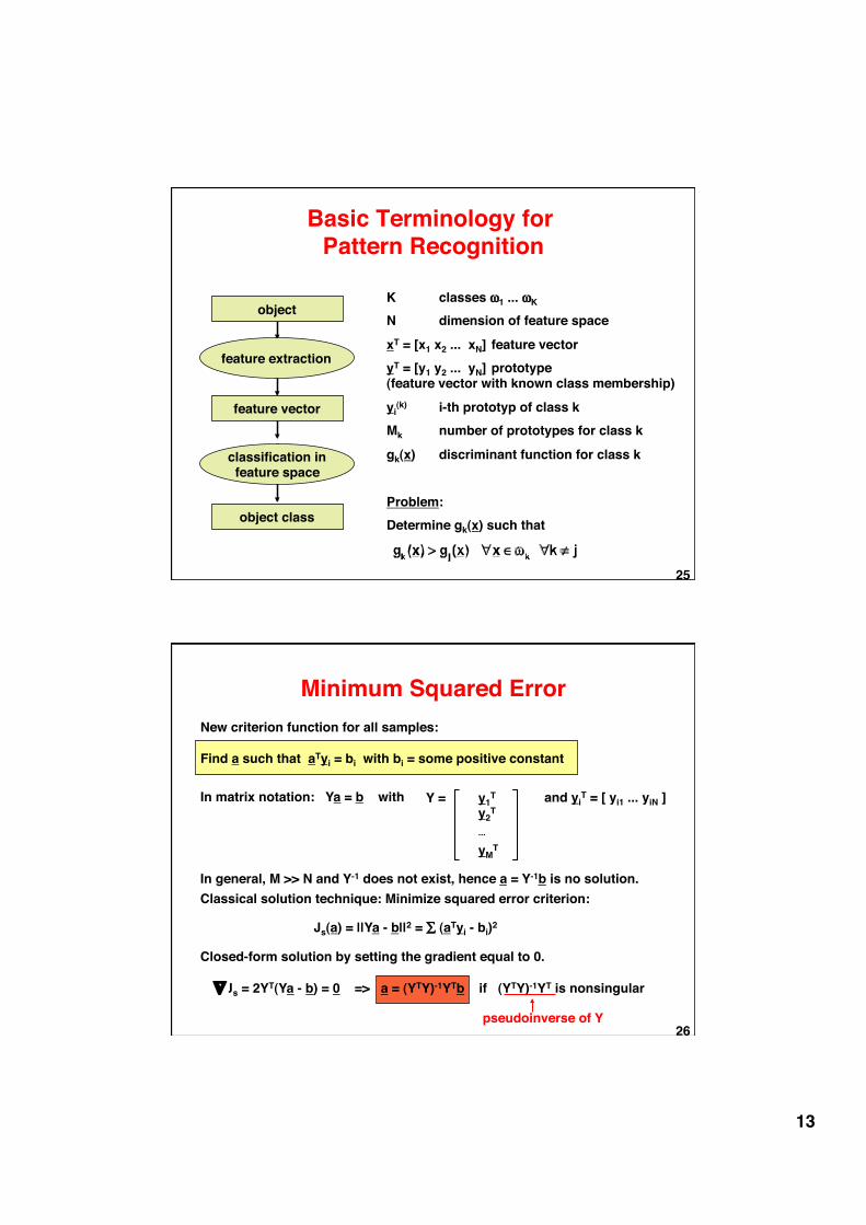
Basic Terminology for Pattern Recognition!
feature extraction!
feature vector!
object!
classification in!feature space!
object class!
K !classes ω1 ... ωK!
N !dimension of feature space!
xT = [x1 x2 ... xN] !feature vector!yT = [y1 y2 ... yN] !prototype!(feature vector with known class membership)!
yi(k) !i-th prototyp of class k!
Mk !number of prototypes for class k!
gk(x) !discriminant function for class k!!
Problem:!Determine gk(x) such that!
26!
Minimum Squared Error!New criterion function for all samples:!!Find a such that aTyi = bi with bi = some positive constant !
In matrix notation: Ya = b with ! Y = !y1T !
!y2T!
!!!...!
!yMT!
and yiT = [ yi1 ... yiN ]!
In general, M >> N and Y-1 does not exist, hence a = Y-1b is no solution.!Classical solution technique: Minimize squared error criterion: !
Js(a) = ||Ya - b||2 = ∑ (aTyi - bi)2!
Closed-form solution by setting the gradient equal to 0.!
„Js = 2YT(Ya - b) = 0 => a = (YTY)-1YTb if (YTY)-1YT is nonsingular!
pseudoinverse of Y!
!

14!
27!
Statistical Decision Theory!
Generating decision functions from a statistical characterization of classes!(as opposed to a characterization by prototypes)!
Advantages:!1. !The classification scheme may be designed to satisfy an objective
optimality criterion: !! !Optimal decisions minimize the probability of error.!
!2. !Statistical descriptions may be much more compact than a collection
of prototypes.!!3. !Some phenomena may only be adequately described using statistics,
e.g. noise.!
28!
General Framework for Bayes Classification!
28!
Statistical decision theory minimizes the probability of error for classifications based on uncertain evidence!
ω1 ... ωK ! !K classes!P(ωk) ! !prior probability that an object of class k will be observed !x = [x1 ... xN] !N-dimensional feature vector of an object!p(x|ωk) ! !conditional probability ("likelihood") of observing x given
! ! !that the object belongs to class ωK!
P(ωk|x) ! !conditional probability ("posterior probability") that an !! ! !object belongs to class ωK given x is observed ! ! !!
Bayes decision rule:!Classify given evidence x as class ω´ such that ω´ minimizes the probability of error P(ω ≠ ω´| x) ! => Choose ω´ which maximizes the posterior probability P(ω | x)!gi(x) = P(ωi|x) are discriminant functions. !

15!
29!
Motion Analysis!
Motion detection!Register locations in an image sequence which have change due to motion!
Moving object detection and tracking!Detect individual moving objects, determine and predict object trajectories, track objects with a moving camera!Derivation of 3D object properties!Determine 3D object shape from multiple views ("shape from motion")!
Motion analysis of digital images is based on a temporal sequence of image frames of a coherent scene.!"sparse sequence" => !few frames, temporally spaced apart, !
! ! !considerable differences between frames!"dense sequence" => !many frames, incremental time steps,!
! ! !incremental differences between frames!video ! ! =>!50 half frames per sec, interleaving, !
! ! !line-by-line sampling!
30!
Kalman Filters (1)!A Kalman filter provides an iterative scheme for (i) predicting an event and (ii) incorporating new measurements. !
prediction! measurement!
Assume a linear system with observations depending linearly on the system state, and white Gaussian noise disturbing the system evolution and the observations:!
xk+1 = Akxk + wk!zk = Hkxk + vk!
xk !quantity of interest ("state") at time k!Ak !model for evolution of xk !wk !zero mean Gaussian noise with
covariance Qk !zk !observations at time k!Hk !relation of observations to state!vk !zero mean Gaussian noise with
covariance Rk !Often, Ak, Qk, Hk and Rk are constant.!
What is the best estimate of xk based on the previous estimate xk-1 and the observation zk?!
16!
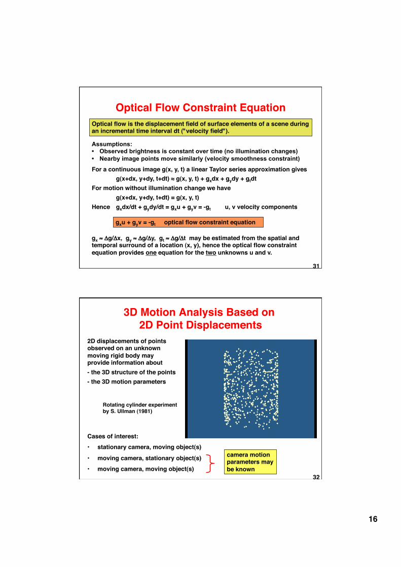
Optical Flow Constraint Equation!Optical flow is the displacement field of surface elements of a scene during an incremental time interval dt ("velocity field").!
Assumptions: • Observed brightness is constant over time (no illumination changes) • Nearby image points move similarly (velocity smoothness constraint)
For a continuous image g(x, y, t) a linear Taylor series approximation gives!!g(x+dx, y+dy, t+dt) ≈ g(x, y, t) + gxdx + gydy + gtdt!
For motion without illumination change we have!!g(x+dx, y+dy, t+dt) = g(x, y, t)!
Hence !gxdx/dt + gydy/dt = gxu + gyv = -gt ! u, v velocity components! !
gxu + gyv = -gt !optical flow constraint equation!
gx ≈ Δg/Δx, gy ≈ Δg/Δy, gt ≈ Δg/Δt may be estimated from the spatial and temporal surround of a location (x, y), hence the optical flow constraint equation provides one equation for the two unknowns u and v. !
31!
32!
3D Motion Analysis Based on 2D Point Displacements!
2D displacements of points observed on an unknown moving rigid body may provide information about !- the 3D structure of the points!- the 3D motion parameters!
Cases of interest:!• !stationary camera, moving object(s)!
• !moving camera, stationary object(s)!• !moving camera, moving object(s)!
camera motion parameters may be known!
Rotating cylinder experiment!by S. Ullman (1981)!

17!
33!
Essential Matrix!Geometrical constraints derived from 2 views of a point in motion!
z!
x!
y!
• vm! • vm+1!Rm!tm!
•!
• !motion between image m and m+1 may be decomposed into!!1) rotation Rm about origin of coordinate system (= optical center)!!2) translation tm!
• !observations are given by direction vectors nm and nm+1 along projection rays!
Rmnm, tm and nm are coplanar: ![tm x Rmnm]T nm+1 = 0!
After some manipulation: !nmT Em nm+1 = 0 E = essential matrix
!
with Em = ! ! !and Rm =!
nm!
nm+1!
tmxr1! tmxr2! tmxr3!
|!!|!
|!!|!
|!!|!
r1 r2 r3!
|!!|!
|!!|!
|!!|!
34!
Principle of Shape from Shading!
Physical surface properties, surface orientation, illumination and viewing direction determine the greyvalue of a surface patch in a sensor signal.!For a single object surface viewed in one image, greyvalue changes are mainly caused by surface orientation changes.!The reconstruction of arbitrary surface shapes is not possible because different surface orientations may give rise to identical greyvalues.!Surface shapes may be uniquely reconstructed from shading information if possible surface shapes are constrained by smoothness assumptions.!
See "Shape from Shading" (B.K.P. Horn, M.J. Brooks, eds.), MIT Press 1989!
a: !patch with known orientation!b, c: !neighbouring patches with similar orientations !b´: !radical different orientation may not be
neighbour of a!
Principle of incremental procedure for surface shape reconstruction:!
a!b!
c!b´!
18!
35!
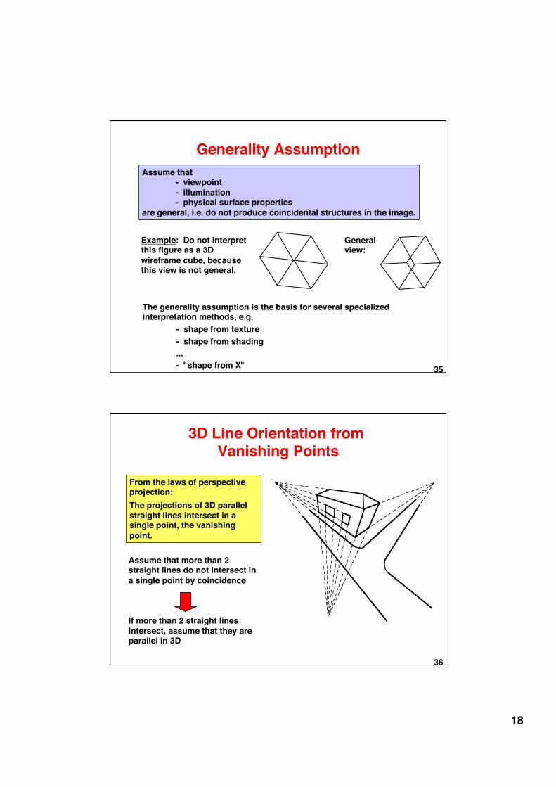
Generality Assumption!Assume that !
!- viewpoint!!- illumination!!- physical surface properties!
are general, i.e. do not produce coincidental structures in the image.!
Example: Do not interpret this figure as a 3D wireframe cube, because this view is not general.!
General view:!
The generality assumption is the basis for several specialized interpretation methods, e.g.!
!- shape from texture!!- shape from shading!!...!!- "shape from X" !
36!
3D Line Orientation from Vanishing Points!
From the laws of perspective projection:!The projections of 3D parallel straight lines intersect in a single point, the vanishing point. !
Assume that more than 2 straight lines do not intersect in a single point by coincidence !!!!If more than 2 straight lines intersect, assume that they are parallel in 3D!

19!
37!
Object Recognition by Relational Matching!
Principle:!• !construct relational model(s) for object class(es)!
• !construct relational image description!• !compute R-morphism (best partial match) between image and
model(s)!
• !top-down verification with extended model !
A!B!
C!D!
E!
F!G!
r1!r2!
r1!
r1!
r3!
r3!
r2!
r4!
r1!r2!
r4!
a
b
c
d e
f!
g
h
i!
j!r1!
r2!r3!
r1!
r2!
r3!
r1!
r4!
r4!
r1!
r2!r2!
r2!r3!
r3!
r1!r1!
r1!
model! image!
38!
SIFT Features Summary
• SIFT features are reasonably invariant to rotation, scaling, and illumination changes.
• They can be used for matching and object recognition (among other things).
• Robust to occlusion: as long as we can see at least 3 features from the object we can compute the location and pose.
• Efficient on-line matching: recognition can be performed in close-to-real time (at least for small object databases).

20!
39!
Basic Building Blocks for High-level Scene Interpretation!
geometrical!scene description (GSD)!
image sequences of dynamic scenes!
high-level !scene interpretations!
scene models!
vision memory!
memory templates!
context information!
40!
Occurrence Models!
• !An occurrence model describes a class of occurrences by!!- !properties!!- !sub-occurrences (= components of the occurrence)!!- !relations between sub-occurrences!
!• !A primitive occurrence model consists of!
!- !properties!!- !a qualitative predicate!
!• !Each occurrence has a begin and end time point !
Basic ingredients: !• !relational structure!! ! ! !• !taxonomy!! ! ! !• !partonomy!! ! ! !• !spatial relational language!! ! ! !• !temporal relational language!! ! ! !• !object appearance models!

21!
41!
Model-based Interpretation!place-cover!
plate!
move!
plate-transport !
transport!
plate-view!
agent! cup!
cup-view!
cup-transport!
agent-view!
agent-move!
move1!move2!
place-cover!
transport2 ! transport1!
plate1!agent1!
view!track!
track2! track1!
view2! view1!
move3!move4!
cup1!
track3!track4!
agent2!
view3!view4!
track4! track3!
part-of!
is-a!
instance!
42!
Causality Graph!Conditional dependencies (causality relations) of random variables define partial order.!Representation as a directed acyclic graph (DAG):!
X7!
X8!X6!
X4!
X5! X3!
X1!
X2!
P(X1, X2, X3, ... , X8) = !P(X1 | X2, X3, X4) • P(X2) • P(X3 | X4, X5) • P(X4 | X6) • P(X5 | X6) • P(X6 | X7X8) • P(X7) • P(X8)!
For any DAG, we obtain the JPD as follows:!!Pa(Xi) !parents of node Xi!
!P(X1 ... XN) = ∏ P(Xi | Pa(Xi))!i!

22!
43!
Example: Traffic Behaviour of Pedestrians!
X4: !pedestrian inattentive!
X3:! car comes!
X2: !pedestrian
light red!
X5: !pedestrian looks
on street!
X1: !pedestrian
enters street!
X6: !traffic light red!
Conditional probability table for each node must be known!
P(X1 | X2, X3, X4, X5) ! P(X2 | X6) ! P(X3 | X6) ! P(X4)! !P(X5) ! P(X6)!
X1 !X2 !X3 !X4 !X5 !P!T !T !T !T !T !0.3!F !T !T !T !T !0.7!T !F !T !T !T !0.9!F !F !T !T !T !0.1!• !• !• !• !• !•!• !• !• !• !• !•!• !• !• !• !• !•!
X2 !X6 !P!T !T !0.2!F !T !0.8!T !F !1.0!F !F !0.0!
X3 !X6 !P!T !T !0.01!F !T !0.99!T !F !0.6!F !F !0.4!
X6 !P!T !0.7!F !0.3!
X4 !P!T !0.1!F !0.9!
X5 !P!T !0.7!F !0.3!
44!
Computing Inferences!We want to use a Bayes Net for probabilistic inferences of the following kind: !
Given a joint probability P(X1, ... , XN) represented by a Bayes Net, and evidence Xm1
=am1, ... , XmK
=amK for some of the variables, what is
the probability P(Xn= ai | Xm1=am1
, ... , XmK=amK
) of an unobserved variable to take on a value ai ?!
! ! ! !P(Xn= ai, Xm1=am1
, ... , XmK=amK
)!P(Xn= ai | Xm1
=am1, ... , XmK
=amK) =!
! ! ! !P(Xm1=am1
, ... , XmK=amK
)!
In general this requires!- !expressing a conditional probability by a quotient of joint probabilities!
- !determining partial joint probabilities from the given total joint probability by summing out unwanted variables!
P(Xm1=am1
, ... , XmK=amK
) = ∑ P(Xm1=am1
, ... , XmK=amK
, Xn1, ... , XnK
)!

23!
45!
What Kind of Bayes Net is a HMM?!
X1! X2! X3! X4!
•••!Y1! Y2! Y3! Y4! •••!
states!!
observations!
Bayes Net structure:!
Finding most probable paths:!
X1! X2! X3! X4!
Y1! Y2! Y3! Y4!
hidden states!!
given observations!
P(X = a | Y = b) = ?!
Evaluating likelihood of model:!
X1! X2! X3! X4!
Y1! Y2! Y3! Y4!
hidden states!!
given observations!
P(Y = b | model) = ?!
46!
How come, you see what you see?!