a vector algebra formulation of mobile robot velocity ...alonzo/pubs/papers/fsr2012.pdf · a vector...

A Vector Algebra Formulation of Mobile RobotVelocity Kinematics

Alonzo Kelly and Neal Seegmiller

Abstract Typical formulations of the forward and inverse velocity kinematics ofwheeled mobile robots assume flat terrain, consistent constraints, and no slip at thewheels. Such assumptions can sometimes permit the wheel constraints to be substi-tuted into the differential equation to produce a compact, apparently unconstrainedresult. However, in the general case, the terrain is not flat, the wheel constraintscannot be eliminated in this way, and they are typically inconsistent if derived fromsensed information. In reality, the motion of a wheeled mobile robot (WMR) is re-stricted to a manifold which more-or-less satisfies the wheel slip constraints whileboth following the terrain and responding to the inputs. To address these more re-alistic cases, we have developed a formulation of WMR velocity kinematics as adifferential-algebraic system — a constrained differential equation of first order.This paper presents the modeling part of the formulation. The Transport Theorem isused to derive a generic 3D model of the motion at the wheels which is implied bythe motion of an arbitrarily articulated body. This wheel equation is the basis for for-ward and inverse velocity kinematics and for the expression of explicit constraints ofwheel slip and terrain following. The result is a mathematically correct method forpredicting motion over non-flat terrain for arbitrary wheeled vehicles on arbitraryterrain subject to arbitrary constraints. We validate our formulation by applying itto a Mars rover prototype with a passive suspension in a context where ground truthmeasurement is easy to obtain. Our approach can constitute a key component ofmore informed state estimation, motion control, and motion planning algorithmsfor wheeled mobile robots.

Alonzo Kelly and Neal SeegmillerRobotics Institute, Carnegie Mellon University, e-mail: alonzo,[email protected]

1

2 Alonzo Kelly and Neal Seegmiller

1 Introduction

Wheeled mobile robots (WMRs) are perhaps the most common configuration of ter-restrial mobile robot, and although decades of research are behind us, little has beenrevealed about how to model them effectively in anything other than flat floor envi-ronments. The motion model of the robot is nonetheless central to pose estimation,control, and motion planning.

Unlike for their predecessors, manipulators, modeling the articulations of themechanisms involved is not the fundamental issue. WMRs need to know how theymove over the terrain and such models are intrinsically differential equations. ForWMRs, these equations are also constrained, the constraints are nonholonomic, thesystem is almost always overconstrained to some degree, and even if it was not, theconstraints are typically violated in ways that are only partially predictable. In thislight, it is perhaps less surprising that so little has been written on this problem.While its importance is clear, its solution is less clear.

Our own historical approaches to the problem [6] have avoided the issues by for-mulating inputs in state space, where constraints (and constraint consistency) are notan issue. Terrain following was treated after the fact by integrating the unconstraineddynamics and then forcing the constraints to be satisfied in a separate optimizationprocess. While this was adequate, it was hardly principled.

While service robots may operate exclusively in flat floor environments, almostany useful field robot will have to operate competently on uneven, sloped, and slip-pery terrain for extended periods of time. The first step toward competent autonomyin these conditions is the incorporation of faster-than-real-time models that predictthe consequences of candidate actions well. Fast and accurate WMR models aretherefore a fundamental problem and we propose a general approach to designingsuch models in this paper.

1.1 Prior Work

Muir and Newman published one of the earliest general approaches to kinematicmodeling of wheeled mobile robots [10]. Following Sheth-Uicker conventions theyassign coordinate systems and derive a graph of homogenous transforms relatingwheel and robot positions. By differentiating cascades of transforms, Jacobian ma-trices are computed for each wheel (relating wheel and robot velocities) which arecombined to form the “composite robot equation.” They provide a “sensed forward”solution (in which the robot velocity is determined from sensed steer angles andwheel velocities) as well as an “actuated inverse” solution.

Several researchers extended this transformation approach to WMR kinematicsmodeling. Alexander and Maddocks proposed an alternative forward solution whenrolling without slipping is impossible, derived from Coulomb’s Law of friction [1].Rajagopalan handled the case of inclined steering columns [11]. Campion et al.classified WMR configurations into five mobility types based on degrees of mobility

A Vector Algebra Formulation of Mobile Robot Velocity Kinematics 3

and steerability, which they define [2]. Yet others proposed geometric approaches toWMR kinematics modeling [5][7].

However, these earlier approaches and analyses are limited to planar motion.More recently in 2005, Tarokh and McDermott published a general approach tomodeling full 6-DOF kinematics for articulated rovers driving on uneven terrain[13]. Their approach resembles Muir and Newman in requiring the derivation of ho-mogenous transform graphs and the differentiation of transforms to compute wheelJacobians. Others have derived and simulated full-3D WMR kinematics on roughterrain with specific objectives, such as mechanisms that enable rolling without slip-ping [4][3], precise localization [8], and control of passively-steered rovers [12].

In contrast to prior transformation and geometric approaches, we derive the kine-matics and constraint equations for WMR using vector algebra. This new approachis intuitive and, unlike [13], does not require differentiation. Our method for propa-gating velocities forward through a kinematic chain is a classical one that has alsobeen used in robot manipulation [9].

2 Kinematics of Wheeled Mobile Robots

In the general case, a wheeled mobile robot may be articulated in various ways andit may roll over arbitrary terrain with any particular wheel lying either on or abovethe nominal terrain surface. Assuming terrain contact is assured by geometry or asuspension, there are two principal difficulties associated with wheeled mobile robot(WMR) kinematic modeling: nonlinearity and overconstraint. Nonlinearity occursin steering control because trigonometric functions of the steer angles appear in themapping between body and wheel velocities. Overconstraint can occur in estimationcontexts where the set of m > n measurements of velocities and/or steer angleslead to an inconsistent solution for the n degrees of velocity freedom available inthe vehicle state vector. This section develops solutions for both the control andestimation problems using a vector algebraic formulation.

We will first develop the basic kinematic relationships between a) the linear andangular velocity of a distinguished coordinate frame on the body of the mobile robotand b) the linear velocity of an arbitrarily positioned point corresponding to a wheel.In contrast to all prior work, we will formulate the transformation using vector al-gebra, leading to a very straightforward expression for even the general case.

2.1 Transport Theorem

The key element of the technique is a basic theorem of physics, commonly used indynamics and inertial navigation theory. Known either as the Coriolis Equation orthe Transport Theorem, it concerns the dependence of measurements in physics onthe state of motion of the observer. The notation u

ba will mean the vector quantity


u of frame a with respect to frame b. Let the letter f refer to a frame of referenceassociated with a fixed observer, whereas m will refer to one associated with a mov-ing observer. Due to their relative, instantaneous angular velocity

ω

fm, our observers

would compute (or measure) different time derivatives of the same vector v that arerelated as follows:

dvdt

∣∣∣f=

dvdt

∣∣∣m+

ω

fm×

v (1)

2.2 Velocity Transformation

Now, let these two frames have an instantaneous relative position of rfm. Suppose

that the moving observer measures the position rmo and velocity v

mo of an object o,

and we wish to know what the fixed observer would measure for the motion of thesame object. The position vectors can be derived from vector addition thus:

rfo =

rmo +

rfm (2)

The time derivative of this position vector, computed in the fixed frame is:

ddt

∣∣∣f(r

fo) =

ddt

∣∣∣f(r

mo +

rfm) =

ddt

∣∣∣f(r

mo )+

ddt

∣∣∣f(r

fm) (3)

Now we can apply the Coriolis equation to the first term on the right to pro-duce the general result for the transformation of apparent velocities of the object obetween two frames of reference undergoing arbitrary relative motion:

vfo =

vmo +

vfm +

ω

fm×

rmo (4)

We have used the fact that, for any frames a and b, ddt

∣∣∣b(r

ba) =

vba.

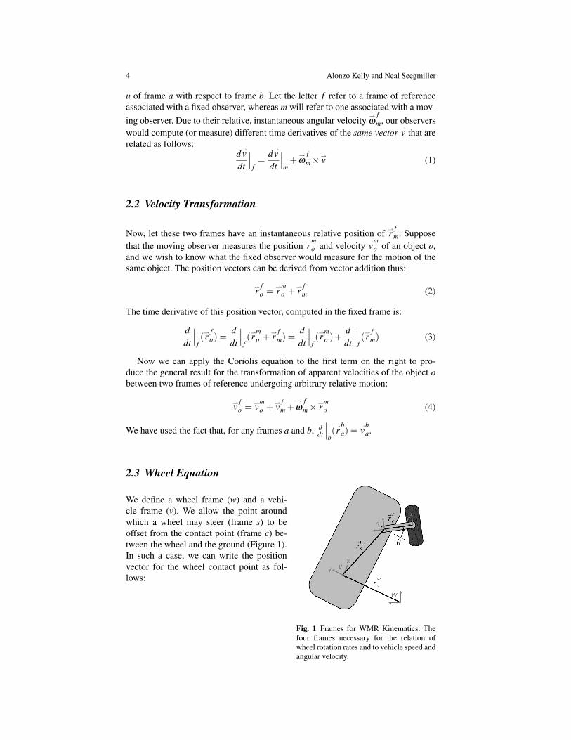
2.3 Wheel Equation

Fig. 1 Frames for WMR Kinematics. Thefour frames necessary for the relation ofwheel rotation rates and to vehicle speed andangular velocity.

We define a wheel frame (w) and a vehi-cle frame (v). We allow the point aroundwhich a wheel may steer (frame s) to beoffset from the contact point (frame c) be-tween the wheel and the ground (Figure 1).In such a case, we can write the positionvector for the wheel contact point as fol-lows:


rwc =

rwv +

rvs +

rsc (5)

Next, we associate any ground-fixed frame with the fixed observer and the body-fixed frame with the moving observer and we can use the above velocity transforma-tion to write a kinematic equation for each wheel. Differentiating the position vectorin the world frame, substituting the Coriolis equation, and using v

vs = 0 yields:

vwc =

vwv +

ω

wv ×

rvs +

ω

wv ×

rsc +

ω

vc×

rsc (6)

This is important enough to give it a name: the wheel equation. In the case of nooffset, the last two terms vanish and the steer velocity (

ω

vs or

ω

vc) no longer matters.

The formula is valid in 3D and it also applies to cases with arbitrary articulationsbetween the v and s frames because only the vector r

vs is relevant. In other words,

this is the general case.

2.4 Inverse Velocity Kinematics - Body to Wheels

Let the term inverse kinematics refer to the problem, relevant to control, of com-puting the wheel velocities from the body velocity. Given the above, the problem issolved by writing a wheel equation for each wheel. To do so, the physical vectorsu must be expressed in a particular coordinate system. Let cub

a denote the vectorquantity u of frame a with respect to frame b, expressed in the coordinates of framec (and let ub

a imply buba). Then, if Rv

s is the rotation matrix that converts coordinatesfrom the steer frame to the vehicle frame, it becomes possible to express the wheelequation for any wheel in the vehicle frame where many of the vectors are typicallyknown:

vvwc = vvw

v + vω

wv × rv

s +vω

wv × Rv

s rsc + ω

vc× Rv

s rsc (7)

2.5 Wheel Steering and Drive - Control and Estimation

In a control context, the wheel equation cannot be used directly as written to findwheel controls because the matrix Rv

s depends on the steer angle, which is one of theunknowns. However, the steer angle can be found by expressing the wheel velocityin wheel coordinates and enforcing the constraint that the lateral (y) component ofthe terrain relative velocity in the wheel frame must vanish. For the geometry inFigure 1, the result is intuitive, the steer angle can be determined from the directionof the s frame because its velocity is parallel to that of c, though not necessarilyof the same magnitude. The velocity of frame s is simply the first two terms of thewheel equation. Then, the steer angle for the wheel is:

θ = atan2[ (vvws )x , (

vvws )y ] (8)


Once the steer angle is known, the wheel velocity along the forward (x) axis of thewheel frame can be determined from the x component the wheel equation in wheelcoordinates. Then the drive velocity (around the axle) can be computed using thewheel radius.

For the opposite problem of wheel sensing, measurements of wheel rotation rateprovide the wheel velocities along the x axis of the wheel frame. Then a measure-ment of steer angle provides the rotation matrix needed to convert to a vector ex-pressed in the vehicle frame.

2.6 Forward Velocity Kinematics - Wheels to Body

Let the term forward kinematics refer to the problem, relevant to estimation, ofcomputing the body velocity from the wheel velocities. The wheel equation canbe written in matrix form by using skew symmetric matrices to represent the crossproducts as a matrix products (specifically, a×b =−b×a =−[b]×a = [b]T×a):

vvwc = vvw

v +[rvs ]

T×(

vω

wv )+ [vrs

c]T×(

vω

wv )+ [vrs

c]T×(ω

vc) (9)

For multiple wheels, stacking all the equations and grouping the first three termstogether produces a matrix equation of the form:

vc = Hv(θ)

[ vvwv

vωwv

]+Hθ (θ)ω

vc = Hv(θ)V +Hθ (θ)θ (10)

where vc represents wheel velocities, and V represents the linear and angular veloc-ity of the vehicle with respect to the ground. Both vc and V are in body coordinates.θ is the steer angles and it can include other articulations if desired. The last term in(10) is the increment to wheel velocity due to the steering rates.

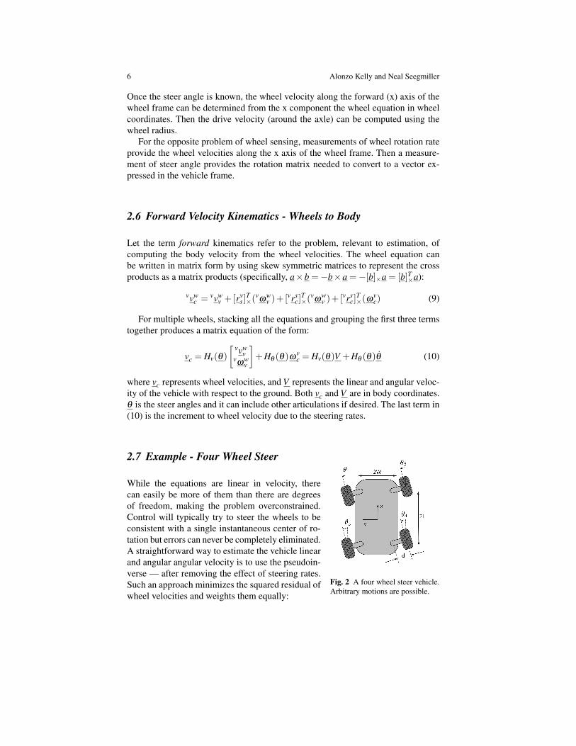
2.7 Example - Four Wheel Steer

Fig. 2 A four wheel steer vehicle.Arbitrary motions are possible.

While the equations are linear in velocity, therecan easily be more of them than there are degreesof freedom, making the problem overconstrained.Control will typically try to steer the wheels to beconsistent with a single instantaneous center of ro-tation but errors can never be completely eliminated.A straightforward way to estimate the vehicle linearand angular angular velocity is to use the pseudoin-verse — after removing the effect of steering rates.Such an approach minimizes the squared residual ofwheel velocities and weights them equally:


V = Hv(θ)+(vc−Hθ (θ)θ) (11)

This case (Figure 2) presents a particularly difficult example of a vehicle withfour wheels which are both driven and steered (from an offset position). The equa-tions were implemented and tested on such a vehicle. Let the velocities of thebody frame in body coordinates be denoted V = [Vx Vy ω]T and the steer anglesθ = [θ1 θ2 θ3 θ4]

T . Unlike a car, this vehicle is not constrained to move in the di-rection it is pointed. Indeed, it can drive with any linear and angular velocity thatis consistent with the wheel speed and steering limits. The steer frame centers arepositioned relative to the body frame as follows:

rvs1 = [L W ]T , rv

s2 = [L −W ]T , rvs3 = [−L W ]T , rv

s4 = [−L −W ]T (12)

The contact point offsets in the body frame depend on the steer angles. They are:

vrs1c1 = d[−s1 c1]

T , vrs2c2 = d[s2 −c2]

T , vrs3c3 = d[−s3 c3]

T , vrs4c4 = d[s4 −c4]

T (13)

where (s1 in the vector denotes sin(θ1) etc.). If we denote the elements of theseposition vectors as rv

s = [x y]T and vrsc = [a b]T , the set of wheel equations is as

follows:

[v1xv1y

]=

[1 0 −(y1 +b1)0 1 (x1 +a1)

]V +

[−b1 0 0 0a1 0 0 0

]θ[

v2xv2y

]=

[1 0 −(y2 +b2)0 1 (x2 +a2)

]V +

[0 −b2 0 00 a2 0 0

]θ (14)[

v3xv3y

]=

[1 0 −(y3 +b3)0 1 (x3 +a3)

]V +

[0 0 −b3 00 0 a3 0

]θ[

v4xv4y

]=

[1 0 −(y4 +b4)0 1 (x4 +a4)

]V +

[0 0 0 −b40 0 0 a4

]θ

3 Wheel Constraints

So far, we have proposed control and estimation mechanisms that satisfy wheelslip constraints in both the forward and inverse kinematics describing the motionof the vehicle in the instantaneous terrain tangent plane. Steering and propulsionare actively controlled in a vehicle, so some measures can be taken to try to satisfywheel slip constraints. Doing so enhances controllability and avoids the energy lossthat would be associated with doing (sliding) work on the terrain.

On non-flat terrain, another constraint of interest is terrain following. Assumingan adequate suspension, wheels should neither penetrate nor rise above the terrain.Such constraints determine altitude (z), and attitude (pitch and roll). These con-


straints are satisfied passively by the suspensions of most vehicles, so the inversekinematic problem of active suspension occurs less often. We will now presentmethods to incorporate both types of constraints in the context of motion predic-tion: the problem of estimating or predicting position and attitude by integrating thesystem differential equation.

3.1 Constrained Dynamics

We will find it convenient to formulate the WMR motion prediction problem as theintegration of a differential-algebraic equation (DAE) where the constraints remainexplicit. We will use a nonstandard formulation of the form:

x = f (x,u)

c(x) = 0 (15)d(x)T x = 0

The m constraint equations in c and d are understood to be active at all times.Each element of d is a particular form of nonholonomic constraint known as a Pfaf-fian velocity constraint. Each specifies a disallowed direction restricting the admis-sible values of the state derivative. The equations in c are holonomic constraints thatrestrict the admissible values of the state x and therefore, through the differentialequation, they ultimately restrict the state derivative as well.

Both forms of constraints are ultimately treated identically because, as is com-monly performed in DAE theory, the gradient of c produces the associated disal-lowed directions of the holonomic constraints. It will turn out that terrain followingwill be expressible as holonomic constraints and wheel slip will be nonholonomic.

3.2 Wheel Slip Constraints

In the case of rolling without lateral slipping, the disallowed direction for the wheelis clearly aligned with the y axis of the contact point c frame. However, to use theconstraint in a DAE, it must be converted to an equivalent disallowed direction instate derivative space. The simplest way to do so is to write (10) in wheel coordinatesthus (assuming Rs

v = Rcv):

cvwc = Rs

vHv(θ)V +RsvHθ (θ)θ (16)

Note that V is exactly the relevant components of the state derivative, so the firstrow of Rs

vHv(θ) is both the gradient of the lateral wheel velocity with respect tothe state derivative, and the associated disallowed direction. Note that in full-3D,


a transformation from Euler angle rates to angular velocity may be required (seeSection 4.1). As long as the steer angles θ are not in the state vector, the secondterm is irrelevant, but if they are, the first row of the gradient can be extracted forthese as well. If there were any other articulations in the kinematic chain from thebody frame to the wheel contact point frame, they can be treated similarly.

3.3 Terrain Following Constraints

It is tempting to extract the z component of the wheel velocity in an analogousmanner to produce a terrain following constraint, but the problem is slightly morecomplicated. It is a basic assumption that the location of the wheel contact pointis known. This point is on the bottom of the wheel on flat terrain and it must becomputed for uneven terrain. In any case, the axes of the c frame are aligned withthe wheel by assumption.

A terrain following constraint can be generated by noting that the terrain normalat the contact point is the other disallowed direction for wheel motion. Indeed, to beprecise, the wheel y axis should ideally be projected onto the terrain tangent planefor lateral slip constraints as well. We can enforce terrain following by requiring thedot product of the terrain normal and contact point velocity vectors to equal zero:n ·vw

c = 0. Accordingly, the gradient of out-of-terrain wheel motion with respect tothe state derivative V is:

d(x)T = vnT Hv(θ) (17)

where vn is the terrain normal expressed in vehicle coordinates.The more common approach (proposed by [16]) is to differentiate the holonomic

constraints c(x) with respect to the state to obtain the gradient cx. The holonomicconstraints are then enforced to first order by requiring that cx x = 0. Here we com-puted the disallowed gradient cx using vector algebra and avoided the differentiation.

4 Results

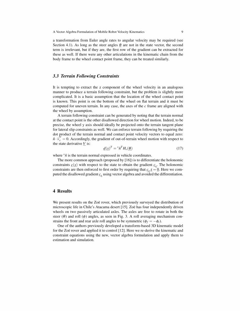
We present results on the Zoe rover, which previously surveyed the distribution ofmicroscopic life in Chile’s Atacama desert [15]. Zoe has four independently drivenwheels on two passively articulated axles. The axles are free to rotate in both thesteer (θ ) and roll (φ ) angles, as seen in Fig. 3. A roll averaging mechanism con-strains the front and rear axle roll angles to be symmetric (φ f =−φr).

One of the authors previously developed a transform-based 3D kinematic modelfor the Zoe rover and applied it to control [12]. Here we re-derive the kinematic andconstraint equations using the new, vector algebra formulation and apply them toestimation and simulation.


Fig. 3 Zoe’s axles are free to rotate in both the steer and roll angles

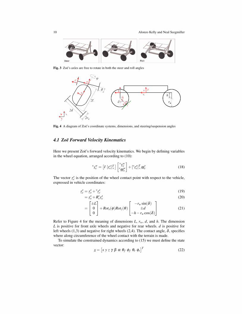
Fig. 4 A diagram of Zoe’s coordinate systems, dimensions, and steering/suspension angles

4.1 Zoe Forward Velocity Kinematics

Here we present Zoe’s forward velocity kinematics. We begin by defining variablesin the wheel equation, arranged according to (10):

vvwc =

[I [rv

c]T×][ vvw

vvωw

v

]+[vrs

c]T×ω

vc (18)

The vector rvc is the position of the wheel contact point with respect to the vehicle,

expressed in vehicle coordinates:

rvc = rv

s +vrs

c (19)= rv

s +Rvs rs

c (20)

=

±L00

+Rotx(φ)Rotz(θ)

−rw sin(δ )±d

−h− rw cos(δ )

(21)

Refer to Figure 4 for the meaning of dimensions L, rw, d, and h. The dimensionL is positive for front axle wheels and negative for rear wheels. d is positive forleft wheels (1,3) and negative for right wheels (2,4). The contact angle, δ , specifieswhere along circumference of the wheel contact with the terrain is made.

To simulate the constrained dynamics according to (15) we must define the statevector:

x =[x y z γ β α θ f φ f θr φr

]T (22)


The first three states are the position of the vehicle in world coordinates (rwv ). The

second three are Euler angles (roll, pitch, and yaw), which specify the orientation ofthe vehicle with respect to the world frame. Let Ω denote the vector of Euler angles:Ω = [γ β α]T . The last four states are the steer (θ ) and roll (φ ) angles for the frontand rear axle joints.

We can compute x from (18), but we must first transform the angular velocitiesto Euler and axle angle rates as follows:

vω

wv = Tωv

γ

β

α

, Tωv =

1 0 −sβ

0 cγ sγcβ

0 −sγ cγcβ

(23)

sω

vs = Tωs

[θ

φ

], Tωs =

001

Rsv

100

(24)

The matrix Tωv (for the Euler angle convention where Rwv =Rotz(α)Roty(β )Rotx(γ))

is widely used in navigation [14]. Given the transforms in (23) and (24) and com-bining wheel equations for all four wheels, we obtain:

vc = Hv(θ)V ′+Hθ (θ)θ (25)vvw

c1...

vvwc4

=

Rvw [rv

c1]T×Tωv

......

Rvw [rv

c4]T×Tωv

[vwv

Ω

]+

[vrs

c1]T×Rv

sTωs 03×2[vrs

c2]T×Rv

sTωs 03×203×2 [vrs

c3]T×Rv

sTωs

03×2 [vrsc4]

T×Rv

sTωs

θ fφ fθrφr

(26)

Each wheel corresponds to three rows of (26). Note that V ′ differs from V as definedin (10) because it contains linear velocities in world coordinates and Euler anglerates Ω . Note also that variables containing s in the superscript or subscript aredifferent for the front and rear axles, i.e. for wheels (1,2) and (3,4).

Because Zoe’s steering and suspension joints are passive, it is necessary in sim-ulation (or prediction) contexts to solve for the joint angle rates θ simultaneouslywith the vehicle velocity V ′:

vc =[Hv(θ) Hθ (θ)

][V ′θ

]= H(θ)x. (27)

The system is overdetermined and can be solved for x using the pseudoinverse.

4.2 Zoe Constraint Equations

As formulated, there are nine total constraints on Zoe’s forward kinematics. As ex-plained in Section 3.2 the nonholonomic, no-lateral-slip constraints are enforced bydisallowing wheel velocity along the y axis of the c frame for each wheel. To com-


pute the constraint for a single wheel, we extract the corresponding 3 rows of (27)and left multiply by Rs

v(= Rcv) to convert to wheel coordinates:

cvwc = Rs

vHc(θ)x (28)

where Hc denotes the three rows of H corresponding to the chosen wheel. The disal-lowed direction in state space d(x)T is simply the second row of Rs

vHc(θ). Because,in this case, left and right wheels on the same axle generate identical no-lateral-slipconstraints, one redundant constraint may be eliminated per axle.

As explained in Section 3.3, the four holonomic terrain following constraints areenforced, to first order, by disallowing wheel velocity in the terrain-normal directionfor each wheel. Given that the dot product vn · vvw

c must be zero, where vn is theterrain normal vector expressed in vehicle (or body) coordinates, the disalloweddirection in state space is vnT Hc.

The roll-averaging mechanism generates one additional holonomic constraintthat φ f +φr = 0. This is enforced to first-order by constraining dφ f

dt + dφrdt = 0.

4.3 Terrain Following Experiment

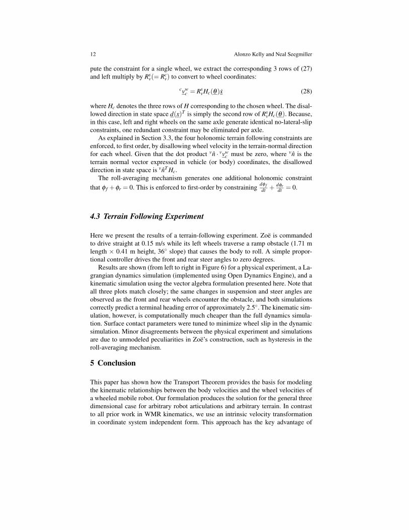
Here we present the results of a terrain-following experiment. Zoe is commandedto drive straight at 0.15 m/s while its left wheels traverse a ramp obstacle (1.71 mlength × 0.41 m height, 36 slope) that causes the body to roll. A simple propor-tional controller drives the front and rear steer angles to zero degrees.

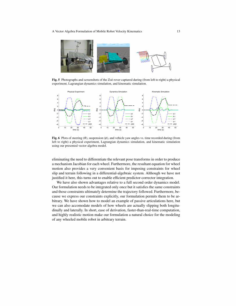
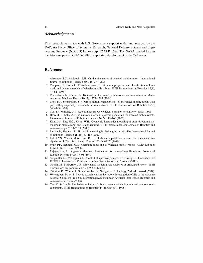
Results are shown (from left to right in Figure 6) for a physical experiment, a La-grangian dynamics simulation (implemented using Open Dynamics Engine), and akinematic simulation using the vector algebra formulation presented here. Note thatall three plots match closely; the same changes in suspension and steer angles areobserved as the front and rear wheels encounter the obstacle, and both simulationscorrectly predict a terminal heading error of approximately 2.5. The kinematic sim-ulation, however, is computationally much cheaper than the full dynamics simula-tion. Surface contact parameters were tuned to minimize wheel slip in the dynamicsimulation. Minor disagreements between the physical experiment and simulationsare due to unmodeled peculiarities in Zoe’s construction, such as hysteresis in theroll-averaging mechanism.

5 Conclusion

This paper has shown how the Transport Theorem provides the basis for modelingthe kinematic relationships between the body velocities and the wheel velocities ofa wheeled mobile robot. Our formulation produces the solution for the general threedimensional case for arbitrary robot articulations and arbitrary terrain. In contrastto all prior work in WMR kinematics, we use an intrinsic velocity transformationin coordinate system independent form. This approach has the key advantage of


Fig. 5 Photographs and screenshots of the Zoe rover captured during (from left to right) a physicalexperiment, Lagrangian dynamics simulation, and kinematic simulation.

0 10 20 30 40 50

−8

−6

−4

−2

0

2

4

6

8

time (s)

de

g

Physical Experiment

θ f

θ r

φ f

φ r

yaw

0 10 20 30 40 50

−8

−6

−4

−2

0

2

4

6

8

time (s)

de

g

Dynamics Simulation

θ f

θ r

φ f

φ r

yaw

0 10 20 30 40 50

−8

−6

−4

−2

0

2

4

6

8

time (s)

de

g

Kinematic Simulation

θ f

θ r

φ f

φ r

yaw

Fig. 6 Plots of steering (θ ), suspension (φ ), and vehicle yaw angles vs. time recorded during (fromleft to right) a physical experiment, Lagrangian dynamics simulation, and kinematic simulationusing our presented vector algebra model.

eliminating the need to differentiate the relevant pose transforms in order to producea mechanism Jacobian for each wheel. Furthermore, the resultant equation for wheelmotion also provides a very convenient basis for imposing constraints for wheelslip and terrain following in a differential-algebraic system. Although we have notjustified it here, this turns out to enable efficient predictor-corrector integration.

We have also shown advantages relative to a full second order dynamics model.Our formulation needs to be integrated only once but it satisfies the same constraintsand those constraints ultimately determine the trajectory followed. Furthermore, be-cause we express our constraints explicitly, our formulation permits them to be ar-bitrary. We have shown how to model an example of passive articulations here, butwe can also accomodate models of how wheels are actually slipping both longitu-dinally and laterally. In short, ease of derivation, faster-than-real-time computation,and highly realistic motion make our formulation a natural choice for the modelingof any wheeled mobile robot in arbitrary terrain.


Acknowledgments

This research was made with U.S. Government support under and awarded by theDoD, Air Force Office of Scientific Research, National Defense Science and Engi-neering Graduate (NDSEG) Fellowship, 32 CFR 168a. The NASA funded Life inthe Atacama project (NAG5-12890) supported development of the Zoe rover.

References

1. Alexander, J.C., Maddocks, J.H.: On the kinematics of wheeled mobile robots. InternationalJournal of Robotics Research 8(5), 15–27 (1989)

2. Campion, G., Bastin, G., D’Andrea-Novel, B.: Structural properties and classification of kine-matic and dynamic models of wheeled mobile robots. IEEE Transactions on Robotics 12(1),47–62 (1996)

3. Chakraborty, N., Ghosal, A.: Kinematics of wheeled mobile robots on uneven terrain. Mech-anism and Machine Theory 39(12), 1273–1287 (2004)

4. Choi, B.J., Sreenivasan, S.V.: Gross motion characteristics of articulated mobile robots withpure rolling capability on smooth uneven surfaces. IEEE Transactions on Robotics 15(2),340–343 (1999)

5. Cox, I.J., Wilfong, G.T.: Autonomous Robot Vehicles. Springer-Verlag, New York (1990)6. Howard, T., Kelly, A.: Optimal rough terrain trajectory generation for wheeled mobile robots.

International Journal of Robotics Research 26(2), 141–166 (2007)7. Kim, D.S., Lee, H.C., Kwon, W.H.: Geometric kinematics modeling of omni-directional au-

tonomous mobile robot and its applications. IEEE International Conference on Robotics andAutomation pp. 2033–2038 (2000)

8. Lamon, P., Siegwart, R.: 3D position tracking in challenging terrain. The International Journalof Robotics Research 26(2), 167–186 (2007)

9. Luh, J.Y.S., Walker, M.W., Paul, R.P.C.: On-line computational scheme for mechanical ma-nipulators. J. Dyn. Sys., Meas., Control 102(2), 69–76 (1980)

10. Muir, P.F., Neuman, C.P.: Kinematic modeling of wheeled mobile robots. CMU RoboticsInstitute Tech. Report (1986)

11. Rajagopalan, R.: A generic kinematic formulation for wheeled mobile robots. Journal ofRobotic Systems 14(2), 77–91 (1997)

12. Seegmiller, N., Wettergreen, D.: Control of a passively steered rover using 3-D kinematics. In:IEEE/RSJ International Conference on Intelligent Robots and Systems (2011)

13. Tarokh, M., McDermott, G.: Kinematics modeling and analyses of articulated rovers. IEEETransactions on Robotics 21(4), 539–553 (2005)

14. Titterton, D., Weston, J.: Strapdown Inertial Navigation Technology, 2nd. edn. AAAI (2004)15. Wettergreen, D., et al.: Second experiments in the robotic investigation of life in the Atacama

desert of Chile. In: Proc. 8th International Symposium on Artificial Intelligence, Robotics andAutomation in Space (2005)

16. Yun, X., Sarkar, N.: Unified formulation of robotic systems with holonomic and nonholonomicconstraints. IEEE Transactions on Robotics 14(4), 640–650 (1998)

a vector algebra formulation of mobile robot velocity ...alonzo/pubs/papers/fsr2012.pdf · a vector...

Documents