a tutorial on particle filtering and smoothing: fifteen ...arnaud/doucet_johansen_tutorialpf.pdf ·...

A Tutorial on Particle Filtering and Smoothing:

Fifteen years later

Arnaud DoucetThe Institute of Statistical Mathematics,

4-6-7 Minami-Azabu, Minato-ku,Tokyo 106-8569, Japan.

Email: [email protected]

Adam M. JohansenDepartment of Statistics,University of Warwick,

Coventry, CV4 7AL, UKEmail: [email protected]

First Version 1.0 – April 2008This Version 1.1 – December 2008

Abstract

Optimal estimation problems for non-linear non-Gaussian state-space models do not typically admitanalytic solutions. Since their introduction in 1993, particle filtering methods have become a verypopular class of algorithms to solve these estimation problems numerically in an online manner, i.e.recursively as observations become available, and are now routinely used in fields as diverse as computervision, econometrics, robotics and navigation. The objective of this tutorial is to provide a complete,up-to-date survey of this field as of 2008. Basic and advanced particle methods for filtering as well assmoothing are presented.

Keywords: Central Limit Theorem, Filtering, Hidden Markov Models, Markov chain Monte Carlo, Par-ticle methods, Resampling, Sequential Monte Carlo, Smoothing, State-Space models.

1 Introduction

The general state space hidden Markov models, which are summarised in section 2.1, provide an extremelyflexible framework for modelling time series. The great descriptive power of these models comes at theexpense of intractability: it is impossible to obtain analytic solutions to the inference problems of interestwith the exception of a small number of particularly simple cases. The “particle” methods described bythis tutorial are a broad and popular class of Monte Carlo algorithms which have been developed overthe past fifteen years to provide approximate solutions to these intractable inference problems.

1.1 Preliminary remarks

Since their introduction in 1993 [22], particle filters have become a very popular class of numerical meth-ods for the solution of optimal estimation problems in non-linear non-Gaussian scenarios. In comparisonwith standard approximation methods, such as the popular Extended Kalman Filter, the principal ad-vantage of particle methods is that they do not rely on any local linearisation technique or any crudefunctional approximation. The price that must be paid for this flexibility is computational: these meth-ods are computationally expensive. However, thanks to the availability of ever-increasing computationalpower, these methods are already used in real-time applications appearing in fields as diverse as chemicalengineering, computer vision, financial econometrics, target tracking and robotics. Moreover, even inscenarios in which there are no real-time constraints, these methods can be a powerful alternative toMarkov chain Monte Carlo (MCMC) algorithms — alternatively, they can be used to design very efficientMCMC schemes.

As a result of the popularity of particle methods, a few tutorials have already been published on thesubject [3, 8, 18, 29]. The most popular, [3], dates back to 2002 and, like the edited volume [16] from2001, it is now somewhat outdated. This tutorial differs from previously published tutorials in two ways.First, the obvious: it is, as of December 2008, the most recent tutorial on the subject and so it has beenpossible to include some very recent material on advanced particle methods for filtering and smoothing.Second, more importantly, this tutorial was not intended to resemble a cookbook. To this end, all of thealgorithms are presented within a simple, unified framework. In particular, we show that essentially allbasic and advanced methods for particle filtering can be reinterpreted as some special instances of a singlegeneric Sequential Monte Carlo (SMC) algorithm. In our opinion, this framework is not only elegant butallows the development of a better intuitive and theoretical understanding of particle methods. It alsoshows that essentially any particle filter can be implemented using a simple computational frameworksuch as that provided by [24]. Absolute beginners might benefit from reading [17], which provides anelementary introduction to the field, before the present tutorial.

1.2 Organisation of the tutorial

The rest of this paper is organised as follows. In Section 2, we present hidden Markov models and theassociated Bayesian recursions for the filtering and smoothing distributions. In Section 3, we introduce ageneric SMC algorithm which provides weighted samples from any sequence of probability distributions.In Section 4, we show how all the (basic and advanced) particle filtering methods developed in theliterature can be interpreted as special instances of the generic SMC algorithm presented in Section 3.Section 5 is devoted to particle smoothing and we mention some open problems in Section 6.

1

2 Bayesian Inference in Hidden Markov Models

2.1 Hidden Markov Models and Inference Aims

Consider an X−valued discrete-time Markov process {Xn}n≥1 such that

X1 ∼ µ (x1) and Xn| (Xn−1 = xn−1) ∼ f (xn|xn−1) (1)

where “∼” means distributed according to, µ (x) is a probability density function and f (x|x′) denotesthe probability density associated with moving from x′ to x. All the densities are with respect to adominating measure that we will denote, with abuse of notation, dx. We are interested in estimating{Xn}n≥1 but only have access to the Y−valued process {Yn}n≥1. We assume that, given {Xn}n≥1,the observations {Yn}n≥1 are statistically independent and their marginal densities (with respect to adominating measure dyn) are given by

Yn| (Xn = xn) ∼ g (yn|xn) . (2)

For the sake of simplicity, we have considered only the homogeneous case here; that is, the transitionand observation densities are independent of the time index n. The extension to the inhomogeneous caseis straightforward. It is assumed throughout that any model parameters are known.

Models compatible with (1)-(2) are known as hidden Markov models (HMM) or general state-space mod-els (SSM). This class includes many models of interest. The following examples provide an illustrationof several simple problems which can be dealt with within this framework. More complicated scenarioscan also be considered.

Example 1 - Finite State-Space HMM. In this case, we have X = {1, ...,K} so

Pr (X1 = k) = µ (k) , Pr (Xn = k|Xn−1 = l) = f (k| l) .

The observations follow an arbitrary model of the form (2). This type of model is extremely generaland examples can be found in areas such as genetics in which they can describe imperfectly observedgenetic sequences, signal processing, and computer science in which they can describe, amongst manyother things, arbitrary finite-state machines.

Example 2 - Linear Gaussian model. Here, X = Rnx , Y = Rny , X1 ∼ N (0,Σ) and

Xn = AXn−1 +BVn,

Yn = CXn +DWn

where Vni.i.d.∼ N (0, Inv

), Wni.i.d.∼ N (0, Inw

) and A,B,C,D are matrices of appropriate dimensions. Notethat N (m,Σ) denotes a Gaussian distribution of mean m and variance-covariance matrix Σ, whereasN (x;m,Σ) denotes the Gaussian density of argument x and similar statistics. In this case µ (x) =N (x; 0,Σ), f (x′|x) = N

(x′;Ax,BBT

)and g (y|x) = N

(y;Cx,DDT

). As inference is analytically

tractable for this model, it has been extremely widely used for problems such as target tracking andsignal processing.

Example 3 - Switching Linear Gaussian model. We have X = U ×Z with U = {1, ...,K} and Z = Rnz .Here Xn = (Un, Zn) where {Un} is a finite state-space Markov chain such that Pr (U1 = k) = µU (k) ,Pr (Un = k|Un−1 = l) = fU (k| l) and conditional upon {Un} we have a linear Gaussian model withZ1|U1 ∼ N (0,ΣU1) and

Zn = AUnZn−1 +BUn

Vn,

Yn = CUnZn +DUn

Wn

2

0 50 100 150 200 250 300 350 400 450 500−15

−10

−5

0

5

10

15Simulated Volatility Sequence

Volatility

Observations

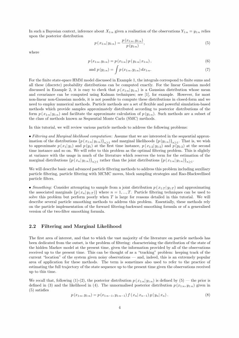
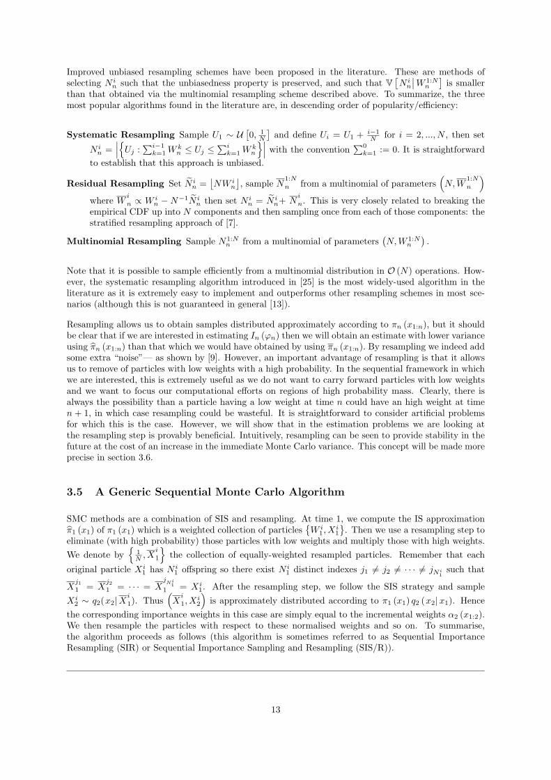
Figure 1: A simulation of the stochastic volatility model described in example 4.

where Vni.i.d.∼ N (0, Inv ), Wn

i.i.d.∼ N (0, Inw ) and {Ak, Bk, Ck, Dk; k = 1, ...,K} are matrices of appropri-ate dimensions. In this case we have µ (x) = µ (u, z) = µU (u)N (z; 0,Σu), f (x′|x) = f ( (u′, z′)| (u, z)) =fU (u′|u)N

(z′;Au′z,Bu′BT

u′

)and g (y|x) = g (y| (u, z)) = N

(y;Cuz,DuD

Tu

). This type of model pro-

vides a generalisation of that described in example 2 with only a slight increase in complexity.

Example 4 - Stochastic Volatility model. We have X = Y = R, X1 ∼ N(

0, σ2

1−α2

)and

Xn = αXn−1 + σVn,

Yn = β exp (Xn/2)Wn

where Vni.i.d.∼ N (0, 1) and Wn

i.i.d.∼ N (0, 1). In this case we have µ (x) = N(x; 0, σ2

1−α2

), f (x′|x) =

N(x′;αx, σ2

)and g (y|x) = N

(y; 0, β2 exp (x)

). Note that this choice of initial distribution ensures that

the marginal distribution of Xn is also µ (x) for all n. This type of model, and its generalisations, havebeen very widely used in various areas of economics and mathematical finance: inferring and predictingunderlying volatility from observed price or rate data is an important problem. Figure 1 shows a shortsection of data simulated from such a model with parameter values α = 0.91, σ = 1.0 and β = 0.5 whichwill be used below to illustrate the behaviour of some simple algorithms.

Equations (1)-(2) define a Bayesian model in which (1) defines the prior distribution of the process ofinterest {Xn}n≥1 and (2) defines the likelihood function; that is:

p (x1:n) = µ (x1)n∏k=2

f (xk|xk−1) (3)

and

p (y1:n|x1:n) =n∏k=1

g (yk|xk) , (4)

where, for any sequence {zn}n≥1, and any i ≤ j, zi:j := (zi, zi+1, ..., zj).

3

In such a Bayesian context, inference about X1:n given a realisation of the observations Y1:n = y1:n reliesupon the posterior distribution

p (x1:n| y1:n) =p (x1:n, y1:n)p (y1:n)

, (5)

where

p (x1:n, y1:n) = p (x1:n) p (y1:n|x1:n) , (6)

and p (y1:n) =∫p (x1:n, y1:n) dx1:n. (7)

For the finite state-space HMM model discussed in Example 1, the integrals correspond to finite sums andall these (discrete) probability distributions can be computed exactly. For the linear Gaussian modeldiscussed in Example 2, it is easy to check that p (x1:n| y1:n) is a Gaussian distribution whose meanand covariance can be computed using Kalman techniques; see [1], for example. However, for mostnon-linear non-Gaussian models, it is not possible to compute these distributions in closed-form and weneed to employ numerical methods. Particle methods are a set of flexible and powerful simulation-basedmethods which provide samples approximately distributed according to posterior distributions of theform p (x1:n| y1:n) and facilitate the approximate calculation of p (y1:n). Such methods are a subset ofthe class of methods known as Sequential Monte Carlo (SMC) methods.

In this tutorial, we will review various particle methods to address the following problems:

• Filtering and Marginal likelihood computation: Assume that we are interested in the sequential approx-imation of the distributions {p (x1:n| y1:n)}n≥1 and marginal likelihoods {p (y1:n)}n≥1. That is, we wishto approximate p (x1| y1) and p (y1) at the first time instance, p (x1:2| y1:2) and p (y1:2) at the secondtime instance and so on. We will refer to this problem as the optimal filtering problem. This is slightlyat variance with the usage in much of the literature which reserves the term for the estimation of themarginal distributions {p (xn| y1:n)}n≥1 rather than the joint distributions {p (x1:n| y1:n)}n≥1.

We will describe basic and advanced particle filtering methods to address this problem including auxiliaryparticle filtering, particle filtering with MCMC moves, block sampling strategies and Rao-Blackwellisedparticle filters.

• Smoothing : Consider attempting to sample from a joint distribution p (x1:T | y1:T ) and approximatingthe associated marginals {p (xn| y1:T )} where n = 1, ..., T . Particle filtering techniques can be used tosolve this problem but perform poorly when T is large for reasons detailed in this tutorial. We willdescribe several particle smoothing methods to address this problem. Essentially, these methods relyon the particle implementation of the forward filtering-backward smoothing formula or of a generalisedversion of the two-filter smoothing formula.

2.2 Filtering and Marginal Likelihood

The first area of interest, and that to which the vast majority of the literature on particle methods hasbeen dedicated from the outset, is the problem of filtering: characterising the distribution of the state ofthe hidden Markov model at the present time, given the information provided by all of the observationsreceived up to the present time. This can be thought of as a “tracking” problem: keeping track of thecurrent “location” of the system given noisy observations — and, indeed, this is an extremely populararea of application for these methods. The term is sometimes also used to refer to the practice ofestimating the full trajectory of the state sequence up to the present time given the observations receivedup to this time.

We recall that, following (1)-(2), the posterior distribution p (x1:n| y1:n) is defined by (5) — the prior isdefined in (3) and the likelihood in (4). The unnormalised posterior distribution p (x1:n, y1:n) given in(5) satisfies

p (x1:n, y1:n) = p (x1:n−1, y1:n−1) f (xn|xn−1) g (yn|xn) . (8)

4

Consequently, the posterior p (x1:n| y1:n) satisfies the following recursion

p (x1:n| y1:n) = p (x1:n−1| y1:n−1)f (xn|xn−1) g (yn|xn)

p (yn| y1:n−1), (9)

wherep (yn| y1:n−1) =

∫p (xn−1| y1:n−1) f (xn|xn−1) g (yn|xn) dxn−1:n (10)

In the literature, the recursion satisfied by the marginal distribution p (xn| y1:n) is often presented. It isstraightforward to check (by integrating out x1:n−1 in (9)) that we have

p (xn| y1:n) =g (yn|xn) p (xn| y1:n−1)

p (yn| y1:n−1), (11)

wherep (xn| y1:n−1) =

∫f (xn|xn−1) p (xn−1| y1:n−1) dxn−1. (12)

Equation (12) is known as the prediction step and (11) is known as the updating step. However, mostparticle filtering methods rely on a numerical approximation of recursion (9) and not of (11)-(12).

If we can compute {p (x1:n| y1:n)} and thus {p (xn| y1:n)} sequentially, then the quantity p (y1:n), whichis known as the marginal likelihood, can also clearly be evaluated recursively using

p (y1:n) = p (y1)n∏k=2

p (yk| y1:k−1) (13)

where p (yk| y1:k−1) is of the form (10).

2.3 Smoothing

One problem, which is closely related to filtering, but computationally more challenging for reasonswhich will become apparent later, is known as smoothing. Whereas filtering corresponds to estimatingthe distribution of the current state of an HMM based upon the observations received up until the currenttime, smoothing corresponds to estimating the distribution of the state at a particular time given allof the observations up to some later time. The trajectory estimates obtained by such methods, as aresult of the additional information available, tend to be smoother than those obtained by filtering. Itis intuitive that if estimates of the state at time n are not required instantly, then better estimationperformance is likely to be obtained by taking advantage of a few later observations. Designing efficientsequential algorithms for the solution of this problem is not quite as straightforward as it might seem,but a number of effective strategies have been developed and are described below.

More formally: assume that we have access to the data y1:T , and wish to compute the marginal distri-butions {p (xn| y1:T )} where n = 1, ..., T or to sample from p (x1:T | y1:T ). In principle, the marginals{p (xn| y1:T )} could be obtained directly by considering the joint distribution p (x1:T | y1:T ) and integrat-ing out the variables (x1:n−1, xn+1:T ). Extending this reasoning in the context of particle methods, onecan simply use the identity p(xn|y1:T ) =

∫p(x1:T |y1:T )dx1:n−1dxn+1:T and take the same approach which

is used in particle filtering: use Monte Carlo algorithms to obtain an approximate characterisation ofthe joint distribution and then use the associated marginal distribution to approximate the distributionsof interest. Unfortunately, as is detailed below, when n � T this strategy is doomed to failure: themarginal distribution p(xn|y1:n) occupies a privileged role within the particle filter framework as it is, insome sense, better characterised than any of the other marginal distributions.

For this reason, it is necessary to develop more sophisticated strategies in order to obtain good smoothingalgorithms. There has been much progress in this direction over the past decade. Below, we present twoalternative recursions that will prove useful when numerical approximations are required. The key to thesuccess of these recursions is that they rely upon only the marginal filtering distributions {p (xn| y1:n)}.

5

2.3.1 Forward-Backward Recursions

The following decomposition of the joint distribution p (x1:T | y1:T )

p (x1:T | y1:T ) = p (xT | y1:T )T−1∏n=1

p (xn|xn+1, y1:T )

= p (xT | y1:T )T−1∏n=1

p (xn|xn+1, y1:n) , (14)

shows that, conditional on y1:T , {Xn} is an inhomogeneous Markov process.

Eq. (14) suggests the following algorithm to sample from p (x1:T | y1:T ). First compute and store themarginal distributions {p (xn| y1:n)} for n = 1, ..., T . Then sample XT ∼ p (xT | y1:T ) and for n =T − 1, T − 2, ..., 1, sample Xn ∼ p (xn|Xn+1, y1:n) where

p (xn|xn+1, y1:n) =f (xn+1|xn) p (xn| y1:n)

p (xn+1| y1:n)

It also follows, by integrating out (x1:n−1, xn+1:T ) in Eq. (14), that

p (xn| y1:T ) = p (xn| y1:n)∫

f (xn+1|xn)p (xn+1| y1:n)

p (xn+1| y1:T ) dxn+1. (15)

So to compute {p (xn| y1:T )}, we simply modify the backward pass and, instead of sampling fromp (xn|xn+1, y1:n), we compute p (xn| y1:T ) using (15).

2.3.2 Generalised Two-Filter Formula

The two-filter formula is a well-established alternative to the forward-filtering backward-smoothing tech-nique to compute the marginal distributions {p (xn| y1:T )} [4]. It relies on the following identity

p (xn| y1:T ) =p (xn| y1:n−1) p (yn:T |xn)

p (yn:T | y1:n−1),

where the so-called backward information filter is initialised at time n = T by p (yT |xT ) = g (yT |xT )and satisfies

p (yn:T |xn) =∫ T∏

k=n+1

f (xk|xk−1)T∏k=n

g (yk|xk) dxn+1:T (16)

= g (yn|xn)∫f (xn+1|xn) p (yn+1:T |xn+1) dxn+1.

The backward information filter is not a probability density in argument xn and it is even possible that∫p (yn:T |xn) dxn =∞. Although this is not an issue when p (yn:T |xn) can be computed exactly, it does

preclude the direct use of SMC methods to estimate this integral. To address this problem, a generalisedversion of the two-filter formula was proposed in [5]. It relies on the introduction of a set of artificialprobability distributions {pn (xn)} and the joint distributions

pn (xn:T | yn:T ) ∝ pn (xn)T∏

k=n+1

f (xk|xk−1)T∏k=n

g (yk|xk) , (17)

which are constructed such that their marginal distributions, pn (xn| yn:T ) ∝ pn (xn) p (yn:T |xn), aresimply “integrable versions” of the backward information filter. It is easy to establish the generalisedtwo-filter formula

p(x1|y1:T ) ∝ µ (x1) p(x1|y1:T )p1 (x1)

, p(xn|y1:T ) ∝ p(xn|y1:n−1)p(xn|yn:T )pn (xn)

(18)

6

which is valid whenever the support of pn (xn) includes the support of the prior pn (xn); that is

pn (xn) =∫µ (x1)

n∏k=2

f (xk|xk−1) dx1:n−1 > 0⇒ pn (xn) > 0.

The generalised two-filter smoother for {p(xn|yn:T )} proceeds as follows. Using the standard forwardrecursion, we can compute and store the marginal distributions {p (xn| y1:n−1)}. Using a backwardrecursion, we compute and store {p(xn|yn:T )}. Then for any n = 1, ..., T we can combine p (xn| y1:n−1)and p(xn|yn:T ) to obtain p(xn|y1:T ).

In [4], this identity is discussed in the particular case where pn (xn) = pn (xn). However, when computing{p(xn|yn:T )} using SMC, it is necessary to be able to compute pn (xn) exactly hence this rules out thechoice pn (xn) = pn (xn) for most non-linear non-Gaussian models. In practice, we should select a heavy-tailed approximation of pn (xn) for pn (xn) in such settings. It is also possible to use the generalised-twofilter formula to sample from p(x1:T |y1:T ); see [5] for details.

2.4 Summary

Bayesian inference in non-linear non-Gaussian dynamic models relies on the sequence of posterior dis-tributions {p (x1:n| y1:n)} and its marginals. Except in simple problems such as Examples 1 and 2, it isnot possible to compute these distributions in closed-form. In some scenarios, it might be possible toobtain reasonable performance by employing functional approximations of these distributions. Here, wewill discuss only Monte Carlo approximations of these distributions; that is numerical schemes in whichthe distributions of interest are approximated by a large collection of N random samples termed parti-cles. The main advantage of such methods is that under weak assumptions they provide asymptotically(i.e. as N → ∞) consistent estimates of the target distributions of interest. It is also noteworthy thatthese techniques can be applied to problems of moderately-high dimension in which traditional numericalintegration might be expected to perform poorly.

3 Sequential Monte Carlo Methods

Over the past fifteen years, particle methods for filtering and smoothing have been the most commonexamples of SMC algorithms. Indeed, it has become traditional to present particle filtering and SMCas being the same thing in much of the literature. Here, we wish to emphasise that SMC actuallyencompasses a broader range of algorithms — and by doing so we are able to show that many moreadvanced techniques for approximate filtering and smoothing can be described using precisely the sameframework and terminology as the basic algorithm.

SMC methods are a general class of Monte Carlo methods that sample sequentially from a sequenceof target probability densities {πn (x1:n)} of increasing dimension where each distribution πn (x1:n) isdefined on the product space Xn. Writing

πn (x1:n) =γn (x1:n)Zn

(19)

we require only that γn : Xn → R+ is known pointwise; the normalising constant

Zn =∫γn (x1:n) dx1:n (20)

might be unknown. SMC provide an approximation of π1 (x1) and an estimate of Z1 at time 1 then anapproximation of π2 (x1:2) and an estimate of Z2 at time 2 and so on.

7

For example, in the context of filtering, we could have γn (x1:n) = p (x1:n, y1:n) , Zn = p (y1:n) soπn (x1:n) = p (x1:n| y1:n). However, we emphasise that this is just one particular choice of target distri-butions. Not only can SMC methods be used outside the filtering context but, more importantly for thistutorial, some advanced particle filtering and smoothing methods discussed below do not rely on thissequence of target distributions. Consequently, we believe that understanding the main principles behindgeneric SMC methods is essential to the development of a proper understanding of particle filtering andsmoothing methods.

We start this section with a very basic review of Monte Carlo methods and Importance Sampling (IS). Wethen present the Sequential Importance Sampling (SIS) method, point out the limitations of this methodand show how resampling techniques can be used to partially mitigate them. Having introduced the basicparticle filter as an SMC method, we show how various advanced techniques which have been developedover the past fifteen years can themselves be interpreted within the same formalism as SMC algorithmsassociated with sequences of distributions which may not coincide with the filtering distributions. Thesealternative sequences of target distributions are either constructed such that they admit the distributions{p (x1:n| y1:n)} as marginal distributions, or an importance sampling correction is necessary to ensurethe consistency of estimates.

3.1 Basics of Monte Carlo Methods

Initially, consider approximating a generic probability density πn (x1:n) for some fixed n. If we sampleN independent random variables, Xi

1:n ∼ πn (x1:n) for i = 1, ..., N , then the Monte Carlo methodapproximates πn (x1:n) by the empirical measure1

πn (x1:n) =1N

N∑i=1

δXi1:n

(x1:n) ,

where δx0 (x) denotes the Dirac delta mass located at x0. Based on this approximation, it is possible toapproximate any marginal, say πn (xk), easily using

πn (xk) =1N

N∑i=1

δXik

(xk) ,

and the expectation of any test function ϕn : Xn → R given by

In (ϕn) :=∫ϕn (x1:n)πn (x1:n) dx1:n,

is estimated by

IMCn (ϕn) :=

∫ϕn (x1:n) πn (x1:n) dx1:n =

1N

N∑i=1

ϕn(Xi

1:n

).

It is easy to check that this estimate is unbiased and that its variance is given by

V[IMCn (ϕn)

]=

1N

(∫ϕ2n (x1:n)πn (x1:n) dx1:n − I2

n (ϕn)).

The main advantage of Monte Carlo methods over standard approximation techniques is that the varianceof the approximation error decreases at a rate of O(1/N) regardless of the dimension of the space Xn.However, there are at least two main problems with this basic Monte Carlo approach:

• Problem 1 : If πn (x1:n) is a complex high-dimensional probability distribution, then we cannot samplefrom it.

1We persist with the abusive use of density notation in the interests of simplicity and accessibility; the alternationsrequired to obtain a rigorous formulation are obvious.

8

• Problem 2 : Even if we knew how to sample exactly from πn (x1:n), the computational complexity ofsuch a sampling scheme is typically at least linear in the number of variables n. So an algorithm samplingexactly from πn (x1:n), sequentially for each value of n, would have a computational complexity increasingat least linearly with n.

3.2 Importance Sampling

We are going to address Problem 1 using the IS method. This is a fundamental Monte Carlo methodand the basis of all the algorithms developed later on. IS relies on the introduction of an importancedensity2 qn (x1:n) such that

πn (x1:n) > 0⇒ qn (x1:n) > 0.

In this case, we have from (19)-(20) the following IS identities

πn (x1:n) =wn (x1:n) qn (x1:n)

Zn, (21)

Zn =∫wn (x1:n) qn (x1:n) dx1:n (22)

where wn (x1:n) is the unnormalised weight function

wn (x1:n) =γn (x1:n)qn (x1:n)

.

In particular, we can select an importance density qn (x1:n) from which it is easy to draw samples; e.g.a multivariate Gaussian. Assume we draw N independent samples Xi

1:n ∼ qn (x1:n) then by insertingthe Monte Carlo approximation of qn (x1:n) — that is the empirical measure of the samples Xi

1:n — into(21)–(22) we obtain

πn (x1:n) =N∑i=1

W inδXi

1:n(x1:n) , (23)

Zn =1N

N∑i=1

wn(Xi

1:n

)(24)

where

W in =

wn(Xi

1:n

)∑Nj=1 wn

(Xj

1:n

) . (25)

Compared to standard Monte Carlo, IS provides an (unbiased) estimate of the normalising constant withrelative variance

VIS

[Zn

]Z2n

=1N

(∫π2n (x1:n)qn (x1:n)

dx1:n − 1). (26)

If we are interested in computing In (ϕn), we can also use the estimate

IISn (ϕn) =

∫ϕn (x1:n) πn (x1:n) dx1:n =

N∑i=1

W inϕn

(Xi

1:n

).

Unlike IMCn (ϕn), this estimate is biased for finite N . However, it is consistent and it is easy to check

that its asymptotic bias is given by

limN→∞

N(IISn (ϕn)− In (ϕn)

)= −

∫π2n (x1:n)qn (x1:n)

(ϕn (x1:n)− In (ϕn)) dx1:n.

2Some authors use the terms proposal density or instrumental density interchangeably.

9

When the normalising constant is known analytically, we can calculate an unbiased importance samplingestimate — however, this generally has higher variance and this is not typically the case in the situationsin which we are interested.

Furthermore, IISn (ϕ) satisfies a Central Limit Theorem (CLT) with asymptotic variance

1N

∫π2n (x1:n)qn (x1:n)

(ϕn (x1:n)− In (ϕn))2dx1:n. (27)

The bias being O(1/N) and the variance O(1/N), the mean-squared error given by the squared bias plusthe variance is asymptotically dominated by the variance term.

For a given test function, ϕn (x1:n), it is easy to establish the importance distribution minimising theasymptotic variance of IIS

n (ϕn). However, such a result is of minimal interest in a filtering context asthis distribution depends on ϕn (x1:n) and we are typically interested in the expectations of several testfunctions. Moreover, even if we were interested in a single test function, say ϕn (x1:n) = xn, then selectingthe optimal importance distribution at time n would have detrimental effects when we will try to obtaina sequential version of the algorithms (the optimal distribution for estimating ϕn−1(x1:n−1) will almostcertainly not be — even similar to — the marginal distribution of x1:n−1 in the optimal distribution forestimating ϕn(x1:n) and this will prove to be problematic).

A more appropriate approach in this context is to attempt to select the qn (x1:n) which minimises thevariance of the importance weights (or, equivalently, the variance of Zn). Clearly, this variance isminimised for qn (x1:n) = πn (x1:n). We cannot select qn (x1:n) = πn (x1:n) as this is the reason weused IS in the first place. However, this simple result indicates that we should aim at selecting an ISdistribution which is close as possible to the target. Also, although it is possible to construct samplersfor which the variance is finite without satisfying this condition, it is advisable to select qn (x1:n) so thatwn (x1:n) < Cn <∞.

3.3 Sequential Importance Sampling

We are now going to present an algorithm that admits a fixed computational complexity at each timestep in important scenarios and thus addresses Problem 2. This solution involves selecting an importancedistribution which has the following structure

qn (x1:n) = qn−1 (x1:n−1) qn (xn|x1:n−1)

= q1 (x1)n∏k=2

qk (xk|x1:k−1) . (28)

Practically, this means that to obtain particles Xi1:n ∼ qn (x1:n) at time n, we sample Xi

1 ∼ q1 (x1) attime 1 then Xi

k ∼ qk(xk|Xi

1:k−1

)at time k for k = 2, ..., n. The associated unnormalised weights can

be computed recursively using the decomposition

wn (x1:n) =γn (x1:n)qn (x1:n)

=γn−1 (x1:n−1)qn−1 (x1:n−1)

γn (x1:n)γn−1 (x1:n−1) qn (xn|x1:n−1)

(29)

which can be written in the form

wn (x1:n) = wn−1 (x1:n−1) · αn (x1:n)

= w1 (x1)n∏k=2

αk (x1:k)

10

where the incremental importance weight function αn (x1:n) is given by

αn (x1:n) =γn (x1:n)

γn−1 (x1:n−1) qn (xn|x1:n−1). (30)

The SIS algorithm proceeds as follows, with each step carried out for i = 1, . . . , N :

Sequential Importance Sampling

At time n = 1

• Sample Xi1 ∼ q1(x1).

• Compute the weights w1

(Xi

1

)and W i

1 ∝ w1

(Xi

1

).

At time n ≥ 2

• Sample Xin ∼ qn(xn|Xi

1:n−1).

• Compute the weights

wn(Xi

1:n

)= wn−1

(Xi

1:n−1

)· αn

(Xi

1:n

),

W in ∝ wn

(Xi

1:n

).

At any time, n, we obtain the estimates πn (x1:n) (Eq. 23) and Zn (Eq. 24) of πn (x1:n) and Zn,respectively. It is straightforward to check that a consistent estimate of Zn/Zn−1 is also provided by thesame set of samples:

ZnZn−1

=N∑i=1

W in−1αn

(Xi

1:n

).

This estimator is motivated by the fact that∫αn (x1:n)πn−1 (x1:n−1) qn(xn|x1:n−1)dx1:n =

∫γn(x1:n)πn−1(x1:n−1)qn(xn|x1:n−1)

γn−1(x1:n−1)qn(xn|x1:n−1)dx1:n =

ZnZn−1

.

In this sequential framework, it would seem that the only freedom the user has at time n is the choice ofqn (xn|x1:n−1)3. A sensible strategy consists of selecting it so as to minimise the variance of wn (x1:n).It is straightforward to check that this is achieved by selecting

qoptn (xn|x1:n−1) = πn (xn|x1:n−1)

as in this case the variance of wn (x1:n) conditional upon x1:n−1 is zero and the associated incrementalweight is given by

αoptn (x1:n) =

γn (x1:n−1)γn−1 (x1:n−1)

=∫γn (x1:n) dxnγn−1 (x1:n−1)

.

Note that it is not always possible to sample from πn (xn|x1:n−1). Nor is it always possible to computeαoptn (x1:n). In these cases, one should employ an approximation of qopt

n (xn|x1:n−1) for qn (xn|x1:n−1).

In those scenarios in which the time required to sample from qn (xn|x1:n−1) and to compute αn (x1:n) isindependent of n (and this is, indeed, the case if qn is chosen sensibly and one is concerned with a problem

3However, as we will see later, the key to many advanced SMC methods is the introduction of a sequence of targetdistributions which differ from the original target distributions.

11

such as filtering), it appears that we have provided a solution for Problem 2. However, it is important tobe aware that the methodology presented here suffers from severe drawbacks. Even for standard IS, thevariance of the resulting estimates increases exponentially with n (as is illustrated below; see also [28]).As SIS is nothing but a special version of IS in which we restrict ourselves to an importance distributionof the form (28) it suffers from the same problem. We demonstrate this using a very simple toy example.

Example. Consider the case where X = R and

πn (x1:n) =n∏k=1

πn (xk) =n∏k=1

N (xk; 0, 1) , (31)

γn (x1:n) =n∏k=1

exp(−x

2k

2

),

Zn = (2π)n/2 .

We select an importance distribution

qn (x1:n) =n∏k=1

qk (xk) =n∏k=1

N(xk; 0, σ2

).

In this case, we have VIS

[Zn

]<∞ only for σ2 > 1

2 and

VIS

[Zn

]Z2n

=1N

[(σ4

2σ2 − 1

)n/2− 1

].

It can easily be checked that σ4

2σ2−1 > 1 for any 12 < σ2 6= 1: the variance increases exponentially with n

even in this simple case. For example, if we select σ2 = 1.2 then we have a reasonably good importance

distribution as qk (xk) ≈ πn (xk) but NVIS[ bZn]Z2

n≈ (1.103)n/2 which is approximately equal to 1.9 × 1021

for n = 1000! We would need to use N ≈ 2× 1023 particles to obtain a relative varianceVIS[ bZn]Z2

n= 0.01.

This is clearly impracticable.

3.4 Resampling

We have seen that IS — and thus SIS — provides estimates whose variance increases, typically expo-nentially, with n. Resampling techniques are a key ingredient of SMC methods which (partially) solvethis problem in some important scenarios.

Resampling is a very intuitive idea which has major practical and theoretical benefits. Consider first anIS approximation πn (x1:n) of the target distribution πn (x1:n). This approximation is based on weightedsamples from qn (x1:n) and does not provide samples approximately distributed according to πn (x1:n) . Toobtain approximate samples from πn (x1:n), we can simply sample from its IS approximation πn (x1:n);that is we select Xi

1:n with probability W in. This operation is called resampling as it corresponds to

sampling from an approximation πn (x1:n) which was itself obtained by sampling. If we are interestedin obtaining N samples from πn (x1:n), then we can simply resample N times from πn (x1:n). This isequivalent to associating a number of offspring N i

n with each particle Xi1:n in such a way that N1:N

n =(N1n, ..., N

Nn

)follow a multinomial distribution with parameter vector

(N,W 1:N

n

)and associating a weight

of 1/N with each offspring. We approximate πn (x1:n) by the resampled empirical measure

πn (x1:n) =N∑i=1

N in

NδXi

1:n(x1:n) (32)

where E[N in

∣∣W 1:Nn

]= NW i

n. Hence πn (x1:n) is an unbiased approximation of πn (x1:n).

12

Improved unbiased resampling schemes have been proposed in the literature. These are methods ofselecting N i

n such that the unbiasedness property is preserved, and such that V[N in

∣∣W 1:Nn

]is smaller

than that obtained via the multinomial resampling scheme described above. To summarize, the threemost popular algorithms found in the literature are, in descending order of popularity/efficiency:

Systematic Resampling Sample U1 ∼ U[0, 1

N

]and define Ui = U1 + i−1

N for i = 2, ..., N , then set

N in =

∣∣∣{Uj :∑i−1k=1W

kn ≤ Uj ≤

∑ik=1W

kn

}∣∣∣ with the convention∑0k=1 := 0. It is straightforward

to establish that this approach is unbiased.

Residual Resampling Set N in =

⌊NW i

n

⌋, sample N

1:N

n from a multinomial of parameters(N,W

1:N

n

)where W

i

n ∝ W in − N−1N i

n then set N in = N i

n+ Ni

n. This is very closely related to breaking theempirical CDF up into N components and then sampling once from each of those components: thestratified resampling approach of [7].

Multinomial Resampling Sample N1:Nn from a multinomial of parameters

(N,W 1:N

n

).

Note that it is possible to sample efficiently from a multinomial distribution in O (N) operations. How-ever, the systematic resampling algorithm introduced in [25] is the most widely-used algorithm in theliterature as it is extremely easy to implement and outperforms other resampling schemes in most sce-narios (although this is not guaranteed in general [13]).

Resampling allows us to obtain samples distributed approximately according to πn (x1:n), but it shouldbe clear that if we are interested in estimating In (ϕn) then we will obtain an estimate with lower varianceusing πn (x1:n) than that which we would have obtained by using πn (x1:n). By resampling we indeed addsome extra “noise”— as shown by [9]. However, an important advantage of resampling is that it allowsus to remove of particles with low weights with a high probability. In the sequential framework in whichwe are interested, this is extremely useful as we do not want to carry forward particles with low weightsand we want to focus our computational efforts on regions of high probability mass. Clearly, there isalways the possibility than a particle having a low weight at time n could have an high weight at timen + 1, in which case resampling could be wasteful. It is straightforward to consider artificial problemsfor which this is the case. However, we will show that in the estimation problems we are looking atthe resampling step is provably beneficial. Intuitively, resampling can be seen to provide stability in thefuture at the cost of an increase in the immediate Monte Carlo variance. This concept will be made moreprecise in section 3.6.

3.5 A Generic Sequential Monte Carlo Algorithm

SMC methods are a combination of SIS and resampling. At time 1, we compute the IS approximationπ1 (x1) of π1 (x1) which is a weighted collection of particles

{W i

1, Xi1

}. Then we use a resampling step to

eliminate (with high probability) those particles with low weights and multiply those with high weights.We denote by

{1N , X

i

1

}the collection of equally-weighted resampled particles. Remember that each

original particle Xi1 has N i

1 offspring so there exist N i1 distinct indexes j1 6= j2 6= · · · 6= jNi

1such that

Xj11 = X

j21 = · · · = X

jNi

11 = Xi

1. After the resampling step, we follow the SIS strategy and sampleXi

2 ∼ q2(x2|Xi

1). Thus(Xi

1, Xi2

)is approximately distributed according to π1 (x1) q2 (x2|x1). Hence

the corresponding importance weights in this case are simply equal to the incremental weights α2 (x1:2).We then resample the particles with respect to these normalised weights and so on. To summarise,the algorithm proceeds as follows (this algorithm is sometimes referred to as Sequential ImportanceResampling (SIR) or Sequential Importance Sampling and Resampling (SIS/R)).

13

Sequential Monte Carlo

At time n = 1



(Xi

1

)and W i

1 ∝ w1

(Xi

1

).

• Resample{W i

1, Xi1

}to obtain N equally-weighted particles

{1N , X

i

1

}.

At time n ≥ 2

• Sample Xin ∼ qn(xn|X

i

1:n−1) and set Xi1:n ←

(Xi

1:n−1, Xin

).

• Compute the weights αn(Xi

1:n

)and W i

n ∝ αn(Xi

1:n

).

• Resample{W in, X

i1:n

}to obtain N new equally-weighted particles

{1N , X

i

1:n

}.

At any time n, this algorithm provides two approximations of πn (x1:n) . We obtain

πn (x1:n) =N∑i=1

W inδXi

1:n(x1:n) (33)

after the sampling step and

πn (x1:n) =1N

N∑i=1

δX

i1:n

(x1:n) (34)

after the resampling step. The approximation (33) is to be preferred to (34). We also obtain anapproximation of Zn/Zn−1 through

ZnZn−1

=1N

N∑i=1

αn(Xi

1:n

).

As we have already mentioned, resampling has the effect of removing particles with low weights andmultiplying particles with high weights. However, this is at the cost of immediately introducing someadditional variance. If particles have unnormalised weights with a small variance then the resamplingstep might be unnecessary. Consequently, in practice, it is more sensible to resample only when thevariance of the unnormalised weights is superior to a pre-specified threshold. This is often assessed bylooking at the variability of the weights using the so-called Effective Sample Size (ESS) criterion [30, pp.35-36], which is given (at time n) by

ESS =

(N∑i=1

(W in

)2)−1

.

Its interpretation is that in a simple IS setting, inference based on the N weighted samples is approxi-mately equivalent (in terms of estimator variance) to inference based on ESS perfect samples from thetarget distribution. The ESS takes values between 1 and N and we resample only when it is below athreshold NT ; typically NT = N/2. Alternative criteria can be used such as the entropy of the weights{W in

}which achieves its maximum value when W i

n = 1N . In this case, we resample when the entropy is

below a given threshold.

14

Sequential Monte Carlo with Adaptive Resampling

At time n = 1



(Xi

1

)and W i

1 ∝ w1

(Xi

1

).

• If resampling criterion satisfied then resample{W i

1, Xi1

}to obtain N equally weighted particles

{1N , X

i

1

}and set

{W

i

1, Xi

1

}←{

1N , X

i

1

}, otherwise set

{W

i

1, Xi

1

}←{W i

1, Xi1

}.

At time n ≥ 2

• Sample Xin ∼ qn(xn|X

i

1:n−1) and set Xi1:n ←

(Xi

1:n−1, Xin

).


1:n

)and W i

n ∝Wi

n−1αn(Xi

1:n

).

• If resampling criterion satisfied, then resample{W in, X

i1:n

}to obtainN equally weighted particles

{1N , X

i

1:n

}and set

{W

i

n, Xi

n

}←{

1N , X

i

n

}, otherwise set

{W

i

n, Xi

n

}←{W in, X

in

}.

In this context too we have two approximations of πn (x1:n)

πn (x1:n) =N∑i=1

W inδXi

1:n(x1:n) , (35)

πn (x1:n) =N∑i=1

Wi

nδXi1:n

(x1:n)

which are equal if no resampling step is used at time n. We may also estimate Zn/Zn−1 through

ZnZn−1

=N∑i=1

Wi

n−1αn(Xi

1:n

). (36)

SMC methods involve systems of particles which interact (via the resampling mechanism) and, conse-quently, obtaining convergence results is a much more difficult task than it is for SIS where standardresults (iid asymptotics) apply. However, there are numerous sharp convergence results available forSMC; see [10] for an introduction to the subject and the monograph of Del Moral [11] for a completetreatment of the subject. An explicit treatment of the case in which resampling is performed adaptivelyis provided by [12].

The presence or absence of degeneracy is the factor which most often determines whether an SMCalgorithm works in practice. However strong the convergence results available for limitingly large samplesmay be, we cannot expect good performance if the finite sample which is actually used is degenerate.Indeed, some degree of degeneracy is inevitable in all but trivial cases: if SMC algorithms are used forsufficiently many time steps every resampling step reduces the number of unique values representing X1,for example. For this reason, any SMC algorithm which relies upon the distribution of full paths x1:n

will fail for large enough n for any finite sample size, N , in spite of the asymptotic justification. It isintuitive that one should endeavour to employ algorithms which do not depend upon the full path ofthe samples, but only upon the distribution of some finite component xn−L:n for some fixed L whichis independent of n. Furthermore, ergodicity (a tendency for the future to be essentially independentof the distant past) of the underlying system will prevent the accumulation of errors over time. Theseconcepts are precisely characterised by existing convergence results, some of the most important of whichare summarised and interpreted in section 3.6.

15

Although sample degeneracy emerges as a consequence of resampling, it is really a manifestation of adeeper problem — one which resampling actually mitigates. It is inherently impossible to accuratelyrepresent a distribution on a space of arbitrarily high dimension with a sample of fixed, finite size. Sampleimpoverishment is a term which is often used to describe the situation in which very few different particleshave significant weight. This problem has much the same effect as sample degeneracy and occurs, inthe absence of resampling, as the inevitable consequence of multiplying together incremental importanceweights from a large number of time steps. It is, of course, not possible to circumvent either problemby increasing the number of samples at every iteration to maintain a constant effective sample size asthis would lead to an exponential growth in the number of samples required. This sheds some light onthe resampling mechanism: it “resets the system” in such a way that its representation of final timemarginals remains well behaved at the expense of further diminishing the quality of the path-samples.By focusing on the fixed-dimensional final time marginals in this way, it allows us to circumvent theproblem of increasing dimensionality.

3.6 Convergence Results for Sequential Monte Carlo Methods

Here, we briefly discuss selected convergence results for SMC. We focus on the CLT as it allows us toclearly understand the benefits of the resampling step and why it “works”. If multinomial resamplingis used at every iteration4, then the associated SMC estimates of Zn/Zn and In (ϕn) satisfy a CLT andtheir respective asymptotic variances are given by

1N

(∫π2n (x1)q1 (x1)

dx1 − 1 +n∑k=2

∫π2n (x1:k)

πk−1 (x1:k−1) qk (xk|x1:k−1)dxk−1:k − 1

)(37)

and∫ π21(x1)q1(x1)

(∫ϕn (x1:n)πn (x2:n|x1) dx2:n − In (ϕn)

)2dx1

+∑n−1k=2

∫ π2n(x1:k)

πk−1(x1:k−1)qk(xk|x1:k−1)

(∫ϕn (x1:n)πn (xk+1:n|x1:k) dxk+1:n − In (ϕn)

)2dx1:k

+∫ π2

n(x1:n)πn−1(x1:n−1)qn(xn|x1:n−1) (ϕn (x1:n)− In (ϕn))2

dx1:n.

(38)

A short and elegant proof of this result is given in [11, Chapter 9]; see also [9]. These expressionare very informative. They show that the resampling step has the effect of “resetting” the particlesystem whenever it is applied. Comparing (26) to (37), we see that the SMC variance expression hasreplaced the importance distribution qn (x1:n) in the SIS variance with the importance distributionsπk−1 (x1:k−1) qk (xk|x1:k−1) obtained after the resampling step at time k − 1. Moreover, we will showthat in important scenarios the variances of SMC estimates are orders of magnitude smaller than thevariances of SIS estimates.

Let us first revisit the toy example discussed in section 3.3.

Example (continued). In this case, it follows from (37) that the asymptotic variance is finite onlywhen σ2 > 1

2 and

VSMC

[Zn

]Z2n

≈ 1N

[∫π2n (x1)q1 (x1)

dx1 − 1 +n∑k=2

∫π2n (xk)qk (xk)

dxk − 1

]

=n

N

[(σ4

2σ2 − 1

)1/2

− 1

]4Similar expressions can be established when a lower variance resampling strategy such as residual resampling is used

and when resampling is performed adaptively [12]. The results presented here are sufficient to guide the design of par-ticular algorithms and the additional complexity involved in considering more general scenarios serves largely to producesubstantially more complex expressions which obscure the important points.

16

compared toVIS

[Zn

]Z2n

=1N

[(σ4

2σ2 − 1

)n/2− 1

].

The asymptotic variance of the SMC estimate increases linearly with n in contrast to the exponentialgrowth of the IS variance. For example, if we select σ2 = 1.2 then we have a reasonably good importancedistribution as qk (xk) ≈ πn (xk). In this case, we saw that it is necessary to employ N ≈ 2 × 1023

particles in order to obtainVIS[ bZn]Z2

n= 10−2 for n = 1000. Whereas to obtain the same performance,

VSMC[ bZn]Z2

n= 10−2, SMC requires the use of just N ≈ 104 particles: an improvement by 19 orders of

magnitude.

This scenario is overly favourable to SMC as the target (31) factorises. However, generally speaking, themajor advantage of SMC over IS is that it allows us to exploit the forgetting properties of the modelunder study as illustrated by the following example.

Example. Consider the following more realistic scenario where

γn (x1:n) = µ (x1)n∏k=2

Mk (xk|xk−1)n∏k=1

Gk (xk)

with µ a probability distribution, Mk a Markov transition kernel and Gk a positive “potential” func-tion. Essentially, filtering corresponds to this model with Mk (xk|xk−1) = f (xk|xk−1) and the timeinhomogeneous potential function Gk(xk) = g (yk|xk). In this case, πk (xk|x1:k−1) = πk (xk|xk−1)and we would typically select an importance distribution qk (xk|x1:k−1) with the same Markov propertyqk (xk|x1:k−1) = qk (xk|xk−1). It follows that (37) is equal to

1N

(∫π2

1 (x1)q1 (x1)

dx1 − 1 +n∑k=2

∫π2n (xk−1:k)

πk−1 (xk−1) qk (xk|xk−1)dxk−1:k − 1

)

and (38), for ϕn (x1:n) = ϕ (xn), equals:∫ π21(x1)q1(x1)

(∫ϕ (xn)πn (xn|x1) dx2:n − In (ϕ)

)2dx1

+∑n−1k=2

∫ π2n(xk−1:k)

πk−1(xk−1)qk(xk|xk−1)

(∫ϕ (xn)πn (xn|xk) dxk − In (ϕ)

)2dxk−1:k

+∫ π2

n(xn−1:n)πn−1(xn−1)qn(xn|xn−1) (ϕ (xn)− In (ϕ))2

dxn−1:n,

where we use the notation In (ϕ) for In (ϕn). In many realistic scenarios, the model associated withπn (x1:n) has some sort of ergodic properties; i.e. ∀xk, x′k ∈ X πn (xn|xk) ≈ πn (xn|x′k) for large enoughn − k. In layman’s terms, at time n what happened at time k is irrelevant if n − k is large enough.Moreover, this often happens exponentially fast; that is for any (xk, x′k)

12

∫|πn (xn|xk)− πn (xn|x′k)| dxn ≤ βn−k

for some β < 1. This property can be used to establish that for bounded functions ϕ ≤ ‖ϕ‖∣∣∣∣∫ ϕ (xn)πn (xn|xk) dxn − I (ϕ)∣∣∣∣ ≤ βn−k ‖ϕ‖

and under weak additional assumptions we have

π2n (xk−1:k)

πk−1 (xk−1) qk (xk|xk−1)≤ A

for a finite constant A. Hence it follows that

VSMC

[Zn

]Z2n

≤ C · nN

,

17

VSMC

[In (ϕ)

]≤ D

N.

for some finite constants C,D that are independent of n. These constants typically increase polynomi-ally/exponentially with the dimension of the state-space X and decrease as β → 0.

3.7 Summary

We have presented a generic SMC algorithm which approximates {πn (x1:n)} and {Zn} sequentially intime.

• Wherever it is possible to sample from qn (xn|x1:n−1) and evaluate αn (x1:n) in a time independentof n, this leads to an algorithm whose computational complexity does not increase with n.

• For any k, there exists n > k such that the SMC approximation of πn (x1:k) consists of a singleparticle because of the successive resampling steps. It is thus impossible to get a “good” SMCapproximation of the joint distributions {πn (x1:n)} when n is too large. This can easily be seen inpractice, by monitoring the number of distinct particles approximating πn (x1).

• However, under mixing conditions, this SMC algorithm is able to provide estimates of marginaldistributions of the form πn (xn−L+1:n) and estimates of Zn/Zn−1 whose variance is uniformlybounded with n. This property is crucial and explains why SMC methods “work” in many realisticscenarios.

• Practically, one should keep in mind that the variance of SMC estimates can only expected to bereasonable if the variance of the incremental weights is small. In particular, this requires that wecan only expect to obtain good performance if πn (x1:n−1) ≈ πn−1 (x1:n−1) and qn (xn|x1:n−1) ≈πn (xn|x1:n−1); that is if the successive distributions we want to approximate do not differ muchone from each other and the importance distribution is a reasonable approximation of the “optimal”importance distribution. However, if successive distributions differ significantly, it is often possibleto design an artificial sequence of distributions to “bridge” this transition [21, 31].

4 Particle Filtering

Remember that in the filtering context, we want to be able to compute a numerical approximationof the distribution {p (x1:n| y1:n)}n≥1 sequentially in time. A direct application of the SMC methodsdescribed earlier to the sequence of target distributions πn (x1:n) = p (x1:n| y1:n) yields a popular classof particle filters. More elaborate sequences of target and proposal distributions yield various moreadvanced algorithms. For ease of presentation, we present algorithms in which we resample at eachtime step. However, in practice we recommend only resampling when the ESS is below a threshold andemploying the systematic resampling scheme.

4.1 SMC for Filtering

First, consider the simplest case in which γn (x1:n) = p (x1:n, y1:n) is chosen, yielding πn (x1:n) =p (x1:n| y1:n) and Zn = p (y1:n). Practically, it is only necessary to select the importance distribu-tion qn (xn|x1:n−1). We have seen that in order to minimise the variance of the importance weights attime n, we should select qopt

n (xn|x1:n−1) = πn (xn|x1:n−1) where

πn (xn|x1:n−1) = p (xn| yn, xn−1)

=g (yn|xn) f (xn|xn−1)

p (yn|xn−1), (39)

18

and the associated incremental importance weight is αn (x1:n) = p (yn|xn−1) . In many scenarios, it isnot possible to sample from this distribution but we should aim to approximate it. In any case, it showsthat we should use an importance distribution of the form

qn (xn|x1:n−1) = q (xn| yn, xn−1) (40)

and that there is nothing to be gained from building importance distributions depending also upon(y1:n−1, x1:n−2) — although, at least in principle, in some settings there may be advantages to usinginformation from subsequent observations if they are available. Combining (29), (30) and (40), theincremental weight is given by

αn (x1:n) = αn (xn−1:n) =g (yn|xn) f (xn|xn−1)

q (xn| yn, xn−1).

The algorithm can thus be summarised as follows.

SIR/SMC for Filtering

At time n = 1

• Sample Xi1 ∼ q(x1| y1).


(Xi

1

)=

µ(Xi1)g(y1|Xi

1)q(Xi

1|y1)and W i

1 ∝ w1

(Xi

1

).

• Resample{W i

1, Xi1


{1N , X

i

1

}.

At time n ≥ 2

• Sample Xin ∼ q(xn| yn, X

i

n−1) and set Xi1:n ←

(Xi

1:n−1, Xin

).

• Compute the weights αn(Xin−1:n

)=

g(yn|Xin)f(Xi

n|Xin−1)

q(Xin|yn,Xi

n−1)and W i

n ∝ αn(Xin−1:n

).


i1:n


{1N , X

i

1:n

}.

We obtain at time n

p (x1:n| y1:n) =N∑i=1

W inδXi

1:n(x1:n) ,

p (yn| y1:n−1) =N∑i=1

W in−1αn

(Xin−1:n

).

However, if we are interested only in approximating the marginal distributions {p (xn| y1:n)} and {p (y1:n)}then we need to store only the terminal-value particles

{Xin−1:n

}to be able to compute the weights: the

algorithm’s storage requirements do not increase over time.

Many techniques have been proposed to design “efficient” importance distributions q (xn| yn, xn−1) whichapproximate p (xn| yn, xn−1). In particular the use of standard suboptimal filtering techniques such asthe Extended Kalman Filter or the Unscented Kalman Filter to obtain importance distributions is verypopular in the literature [14, 37]. The use of local optimisation techniques to design q (xn| yn, xn−1)centred around the mode of p (xn| yn, xn−1) has also been advocated [33, 34].

19

0 10 20 30 40 50 60 70 80 90 100−6

−4

−2

0

2

4

6SV Model: SIS Filtering Estimates

True Volatility

Filter Mean

+/− 1 S.D.

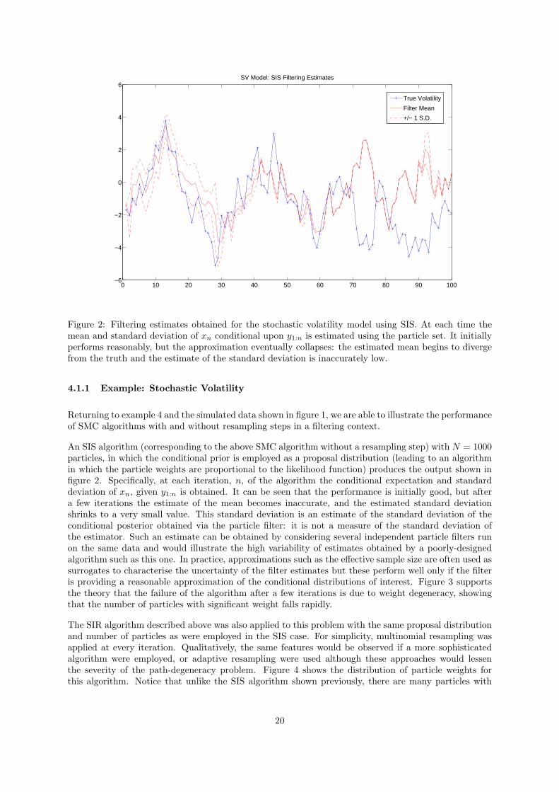
Figure 2: Filtering estimates obtained for the stochastic volatility model using SIS. At each time themean and standard deviation of xn conditional upon y1:n is estimated using the particle set. It initiallyperforms reasonably, but the approximation eventually collapses: the estimated mean begins to divergefrom the truth and the estimate of the standard deviation is inaccurately low.

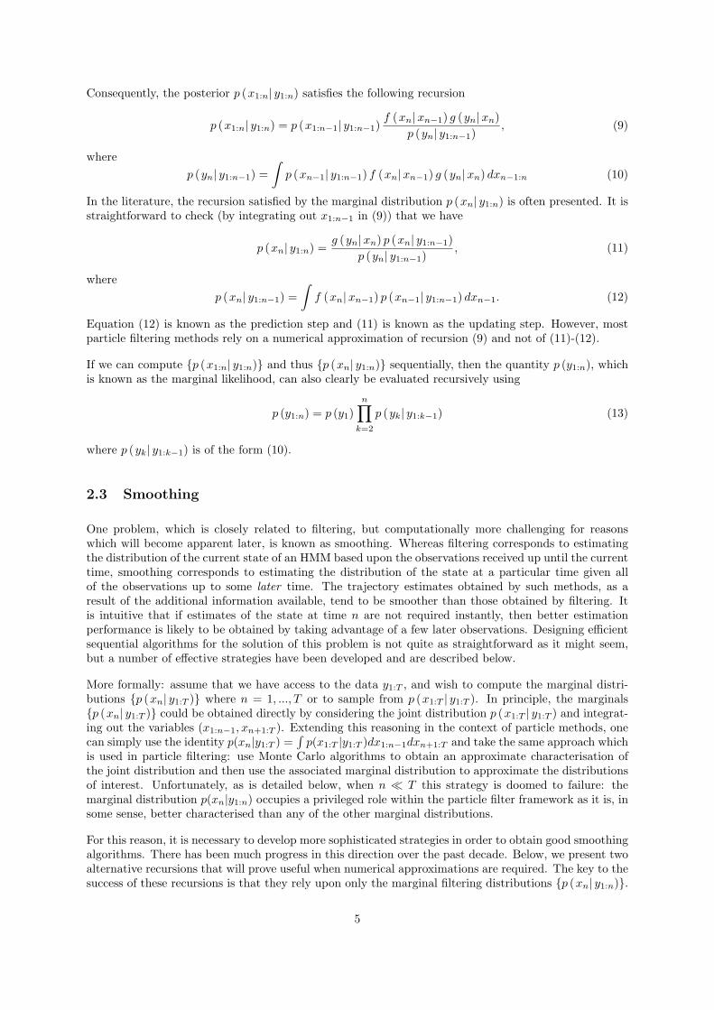
4.1.1 Example: Stochastic Volatility

Returning to example 4 and the simulated data shown in figure 1, we are able to illustrate the performanceof SMC algorithms with and without resampling steps in a filtering context.

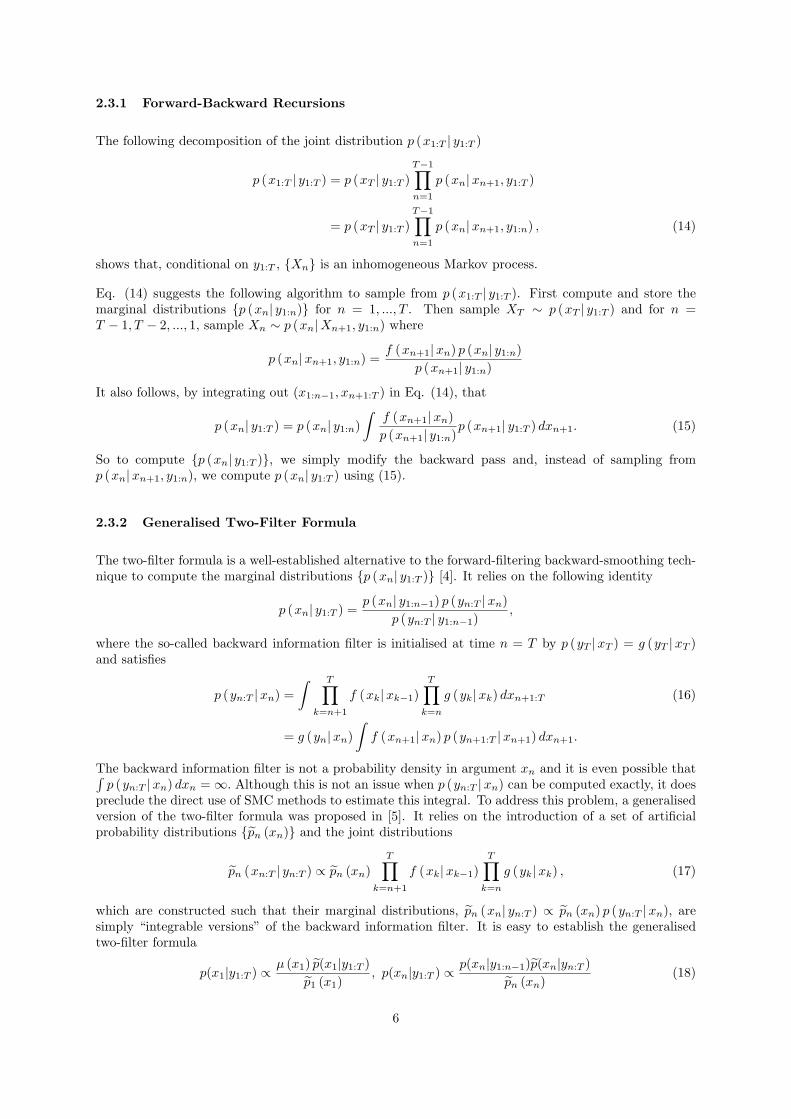
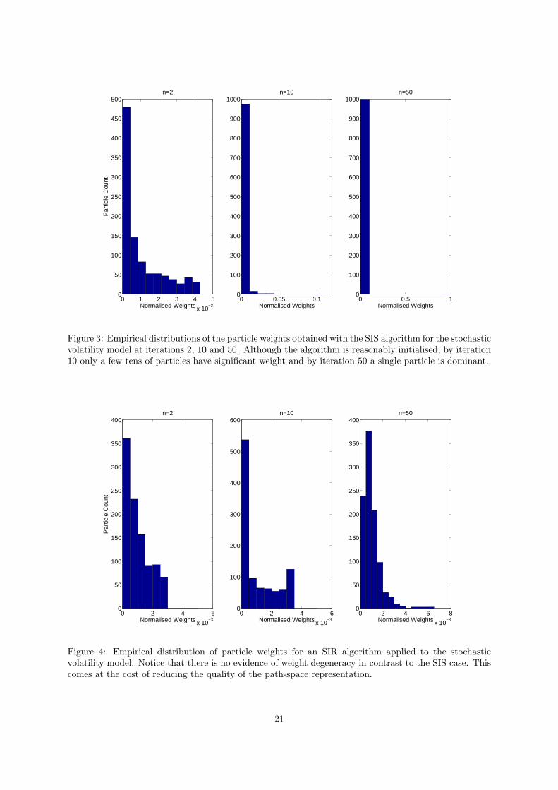
An SIS algorithm (corresponding to the above SMC algorithm without a resampling step) with N = 1000particles, in which the conditional prior is employed as a proposal distribution (leading to an algorithmin which the particle weights are proportional to the likelihood function) produces the output shown infigure 2. Specifically, at each iteration, n, of the algorithm the conditional expectation and standarddeviation of xn, given y1:n is obtained. It can be seen that the performance is initially good, but aftera few iterations the estimate of the mean becomes inaccurate, and the estimated standard deviationshrinks to a very small value. This standard deviation is an estimate of the standard deviation of theconditional posterior obtained via the particle filter: it is not a measure of the standard deviation ofthe estimator. Such an estimate can be obtained by considering several independent particle filters runon the same data and would illustrate the high variability of estimates obtained by a poorly-designedalgorithm such as this one. In practice, approximations such as the effective sample size are often used assurrogates to characterise the uncertainty of the filter estimates but these perform well only if the filteris providing a reasonable approximation of the conditional distributions of interest. Figure 3 supportsthe theory that the failure of the algorithm after a few iterations is due to weight degeneracy, showingthat the number of particles with significant weight falls rapidly.

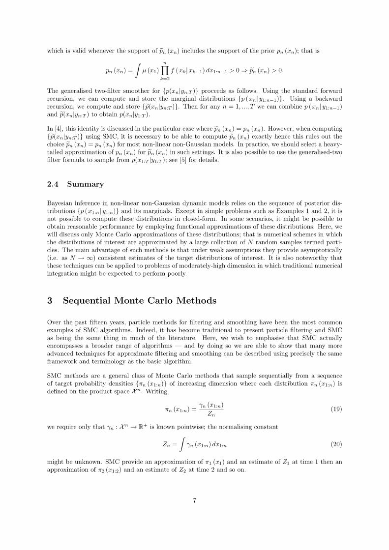
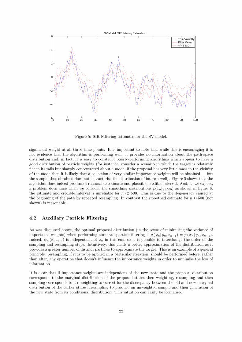
The SIR algorithm described above was also applied to this problem with the same proposal distributionand number of particles as were employed in the SIS case. For simplicity, multinomial resampling wasapplied at every iteration. Qualitatively, the same features would be observed if a more sophisticatedalgorithm were employed, or adaptive resampling were used although these approaches would lessenthe severity of the path-degeneracy problem. Figure 4 shows the distribution of particle weights forthis algorithm. Notice that unlike the SIS algorithm shown previously, there are many particles with

20

0 1 2 3 4 5

x 10−3

0

50

100

150

200

250

300

350

400

450

500n=2

Par

ticle

Cou

nt

Normalised Weights0 0.05 0.1

0

100

200

300

400

500

600

700

800

900

1000n=10

Normalised Weights0 0.5 1

0

100

200

300

400

500

600

700

800

900

1000n=50

Normalised Weights

Figure 3: Empirical distributions of the particle weights obtained with the SIS algorithm for the stochasticvolatility model at iterations 2, 10 and 50. Although the algorithm is reasonably initialised, by iteration10 only a few tens of particles have significant weight and by iteration 50 a single particle is dominant.

0 2 4 6

x 10−3

0

50

100

150

200

250

300

350

400n=2

Par

ticle

Cou

nt

Normalised Weights0 2 4 6

x 10−3

0

100

200

300

400

500

600n=10

Normalised Weights0 2 4 6 8

x 10−3

0

50

100

150

200

250

300

350

400n=50

Normalised Weights

Figure 4: Empirical distribution of particle weights for an SIR algorithm applied to the stochasticvolatility model. Notice that there is no evidence of weight degeneracy in contrast to the SIS case. Thiscomes at the cost of reducing the quality of the path-space representation.

21

0 10 20 30 40 50 60 70 80 90 100−6

−4

−2

0

2

4

6SV Model: SIR Filtering Estimates

True VolatilityFilter Mean+/− 1 S.D.

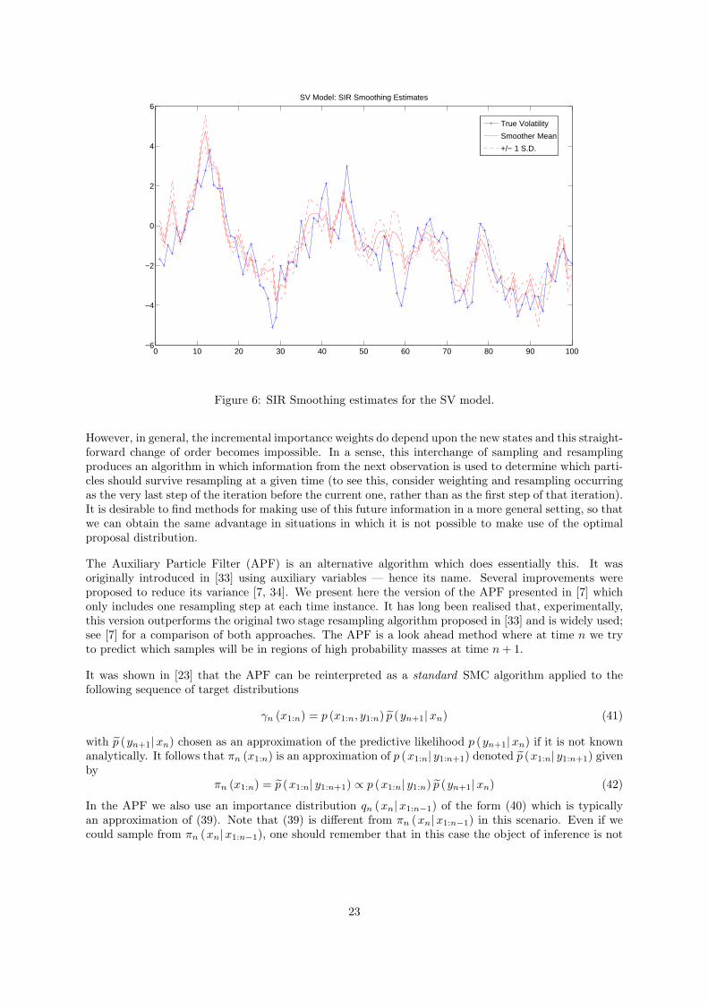
Figure 5: SIR Filtering estimates for the SV model.

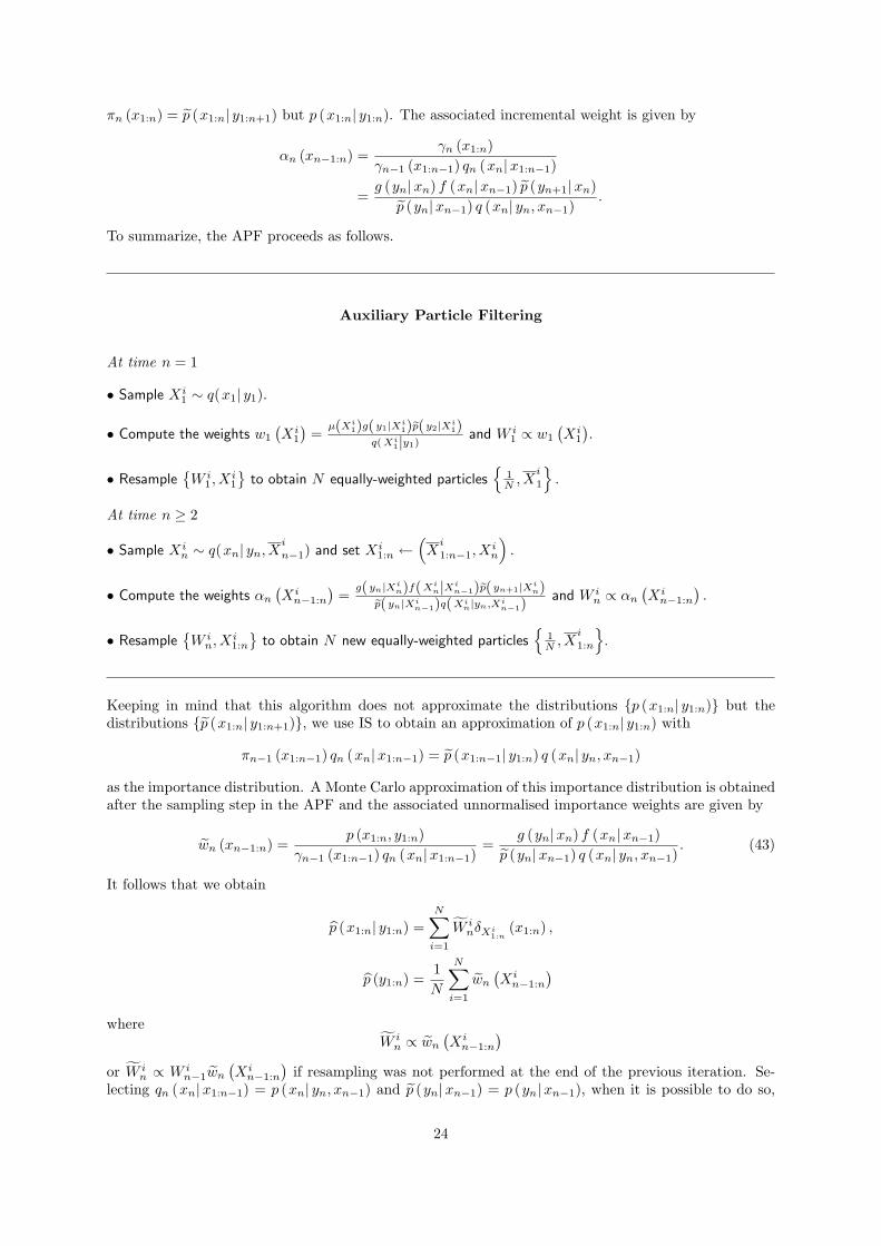
significant weight at all three time points. It is important to note that while this is encouraging it isnot evidence that the algorithm is performing well: it provides no information about the path-spacedistribution and, in fact, it is easy to construct poorly-performing algorithms which appear to have agood distribution of particle weights (for instance, consider a scenario in which the target is relativelyflat in its tails but sharply concentrated about a mode; if the proposal has very little mass in the vicinityof the mode then it is likely that a collection of very similar importance weights will be obtained — butthe sample thus obtained does not characterise the distribution of interest well). Figure 5 shows that thealgorithm does indeed produce a reasonable estimate and plausible credible interval. And, as we expect,a problem does arise when we consider the smoothing distributions p(xn|y1:500) as shown in figure 6:the estimate and credible interval is unreliable for n � 500. This is due to the degeneracy caused atthe beginning of the path by repeated resampling. In contrast the smoothed estimate for n ≈ 500 (notshown) is reasonable.

4.2 Auxiliary Particle Filtering

As was discussed above, the optimal proposal distribution (in the sense of minimising the variance ofimportance weights) when performing standard particle filtering is q (xn| yn, xn−1) = p (xn| yn, xn−1).Indeed, αn (xn−1:n) is independent of xn in this case so it is possible to interchange the order of thesampling and resampling steps. Intuitively, this yields a better approximation of the distribution as itprovides a greater number of distinct particles to approximate the target. This is an example of a generalprinciple: resampling, if it is to be applied in a particular iteration, should be performed before, ratherthan after, any operation that doesn’t influence the importance weights in order to minimise the loss ofinformation.

It is clear that if importance weights are independent of the new state and the proposal distributioncorresponds to the marginal distribution of the proposed states then weighting, resampling and thensampling corresponds to a reweighting to correct for the discrepancy between the old and new marginaldistribution of the earlier states, resampling to produce an unweighted sample and then generation ofthe new state from its conditional distribution. This intuition can easily be formalised.

22

0 10 20 30 40 50 60 70 80 90 100−6

−4

−2

0

2

4

6SV Model: SIR Smoothing Estimates

True Volatility

Smoother Mean

+/− 1 S.D.

Figure 6: SIR Smoothing estimates for the SV model.

However, in general, the incremental importance weights do depend upon the new states and this straight-forward change of order becomes impossible. In a sense, this interchange of sampling and resamplingproduces an algorithm in which information from the next observation is used to determine which parti-cles should survive resampling at a given time (to see this, consider weighting and resampling occurringas the very last step of the iteration before the current one, rather than as the first step of that iteration).It is desirable to find methods for making use of this future information in a more general setting, so thatwe can obtain the same advantage in situations in which it is not possible to make use of the optimalproposal distribution.

The Auxiliary Particle Filter (APF) is an alternative algorithm which does essentially this. It wasoriginally introduced in [33] using auxiliary variables — hence its name. Several improvements wereproposed to reduce its variance [7, 34]. We present here the version of the APF presented in [7] whichonly includes one resampling step at each time instance. It has long been realised that, experimentally,this version outperforms the original two stage resampling algorithm proposed in [33] and is widely used;see [7] for a comparison of both approaches. The APF is a look ahead method where at time n we tryto predict which samples will be in regions of high probability masses at time n+ 1.

It was shown in [23] that the APF can be reinterpreted as a standard SMC algorithm applied to thefollowing sequence of target distributions

γn (x1:n) = p (x1:n, y1:n) p (yn+1|xn) (41)

with p (yn+1|xn) chosen as an approximation of the predictive likelihood p (yn+1|xn) if it is not knownanalytically. It follows that πn (x1:n) is an approximation of p (x1:n| y1:n+1) denoted p (x1:n| y1:n+1) givenby

πn (x1:n) = p (x1:n| y1:n+1) ∝ p (x1:n| y1:n) p (yn+1|xn) (42)

In the APF we also use an importance distribution qn (xn|x1:n−1) of the form (40) which is typicallyan approximation of (39). Note that (39) is different from πn (xn|x1:n−1) in this scenario. Even if wecould sample from πn (xn|x1:n−1), one should remember that in this case the object of inference is not

23

πn (x1:n) = p (x1:n| y1:n+1) but p (x1:n| y1:n). The associated incremental weight is given by

αn (xn−1:n) =γn (x1:n)

γn−1 (x1:n−1) qn (xn|x1:n−1)

=g (yn|xn) f (xn|xn−1) p (yn+1|xn)

p (yn|xn−1) q (xn| yn, xn−1).

To summarize, the APF proceeds as follows.

Auxiliary Particle Filtering

At time n = 1



(Xi

1

)=

µ(Xi1)g(y1|Xi

1)ep(y2|Xi1)

q(Xi1|y1)

and W i1 ∝ w1

(Xi

1

).

• Resample{W i

1, Xi1


{1N , X

i

1

}.

At time n ≥ 2

• Sample Xin ∼ q(xn| yn, X

i

n−1) and set Xi1:n ←

(Xi

1:n−1, Xin

).


)=

g(yn|Xin)f(Xi

n|Xin−1)ep(yn+1|Xi

n)ep(yn|Xin−1)q(Xi

n|yn,Xin−1)

and W in ∝ αn

(Xin−1:n

).


i1:n


{1N , X

i

1:n

}.

Keeping in mind that this algorithm does not approximate the distributions {p (x1:n| y1:n)} but thedistributions {p (x1:n| y1:n+1)}, we use IS to obtain an approximation of p (x1:n| y1:n) with

πn−1 (x1:n−1) qn (xn|x1:n−1) = p (x1:n−1| y1:n) q (xn| yn, xn−1)

as the importance distribution. A Monte Carlo approximation of this importance distribution is obtainedafter the sampling step in the APF and the associated unnormalised importance weights are given by

wn (xn−1:n) =p (x1:n, y1:n)

γn−1 (x1:n−1) qn (xn|x1:n−1)=

g (yn|xn) f (xn|xn−1)p (yn|xn−1) q (xn| yn, xn−1)

. (43)

It follows that we obtain

p (x1:n| y1:n) =N∑i=1

W inδXi

1:n(x1:n) ,

p (y1:n) =1N

N∑i=1

wn(Xin−1:n

)where

W in ∝ wn

(Xin−1:n

)or W i

n ∝ W in−1wn

(Xin−1:n

)if resampling was not performed at the end of the previous iteration. Se-

lecting qn (xn|x1:n−1) = p (xn| yn, xn−1) and p (yn|xn−1) = p (yn|xn−1), when it is possible to do so,

24

leads to the so-called “perfect adaptation” case [33]. In this case, the APF takes a particularly simpleform as αn (xn−1:n) = p (yn|xn−1) and wn (xn−1:n) = 1. This is similar to the algorithm discussed inthe previous subsection where the order of the sampling and resampling steps is interchanged.

This simple reinterpretation of the APF shows us several things:

• We should select a distribution p (x1:n| y1:n) with thicker tails than p (x1:n| y1:n).

• Setting p (yn|xn−1) = g (yn|µ (xn−1)) where µ denotes some point estimate is perhaps unwise asthis will not generally satisfy that requirement.

• We should use an approximation of the predictive likelihood which is compatible with the modelwe are using in the sense that it encodes at least the same degree of uncertainty as the exact model.

These observations follows from the fact that p (x1:n| y1:n) is used as an importance distribution toestimate p (x1:n| y1:n) and this is the usual method to ensure that the estimator variance remains finite.Thus p (yn|xn−1) should be more diffuse than p (yn|xn−1).

It has been suggested in the literature to set p (yn|xn−1) = g (yn|µ (xn−1)) where µ (xn−1) correspondsto the mode, mean or median of f (xn|xn−1). However, this simple approximation will often yield animportance weight function (43) which is not upper bounded on X × X and could lead to estimates witha large/infinite variance.

An alternative approach, selecting an approximation p (yn, xn|xn−1) = p (yn|xn−1) q (xn| yn, xn−1) ofthe distribution p (yn, xn|xn−1) = p (yn|xn−1) p (xn| yn, xn−1) = g (yn|xn) f (xn|xn−1) such that theratio (43) is upper bounded on X × X and such that it is possible to compute p (yn|xn−1) pointwise andto sample from q (xn| yn, xn−1), should be preferred.

4.3 Limitations of Particle Filters

The algorithms described earlier suffer from several limitations. It is important to emphasise at this pointthat, even if the optimal importance distribution p (xn| yn, xn−1) can be used, this does not guaranteethat the SMC algorithms will be efficient. Indeed, if the variance of p (yn|xn−1) is high, then thevariance of the resulting approximation will be high. Consequently, it will be necessary to resamplevery frequently and the particle approximation p (x1:n| y1:n) of the joint distribution p (x1:n| y1:n) willbe unreliable. In particular, for k � n the marginal distribution p (x1:k| y1:n) will only be approximatedby a few if not a single unique particle because the algorithm will have resampled many times betweentimes k and n. One major problem with the approaches discussed above is that only the variables

{Xin

}are sampled at time n but the path values

{Xi

1:n−1

}remain fixed. An obvious way to improve upon

these algorithms would involve not only sampling{Xin

}at time n, but also modifying the values of the

paths over a fixed lag{Xin−L+1:n−1

}for L > 1 in light of the new observation yn; L being fixed or upper

bounded to ensure that we have a sequential algorithm (i.e. one whose computational cost and storagerequirements are uniformly bounded over time). The following two sections describe two approaches tolimit this degeneracy problem.

4.4 Resample-Move

This degeneracy problem has historically been addressed most often using the Resample-Move algorithm[20]. Like Markov Chain Monte Carlo (MCMC), it relies upon Markov kernels with appropriate invari-ant distributions. Whilst MCMC uses such kernels to generate collections of correlated samples, theResample-Move algorithm uses them within an SMC algorithm as a principled way to “jitter” the par-ticle locations and thus to reduce degeneracy. A Markov kernel Kn (x′1:n|x1:n) of invariant distribution

25

p (x1:n| y1:n) is a Markov transition kernel with the property that∫p (x1:n| y1:n)Kn (x′1:n|x1:n) dx1:n = p (x′1:n| y1:n) .

For such a kernel, if X1:n ∼ p (x1:n| y1:n) and X ′1:n|X1:n ∼ K (x1:n|X1:n) then X ′1:n is still marginallydistributed according to p (x1:n| y1:n). Even if X1:n is not distributed according to p (x1:n| y1:n) then,after an application of the MCMC kernel, X ′1:n can only have a distribution closer than that of X1:n

(in total variation norm) to p (x1:n| y1:n). A Markov kernel is said to be ergodic if iterative applicationof that kernel generates samples whose distribution converges towards p (x1:n| y1:n) irrespective of thedistribution of the initial state.

It is easy to construct a Markov kernel with a specified invariant distribution. Indeed, this is thebasis of MCMC — for details see [35] and references therein. For example, we could consider thefollowing kernel, based upon the Gibbs sampler: set x′1:n−L = x1:n−L then sample x′n−L+1 fromp(xn−L+1| y1:n, x

′1:n−L, xn−L+2:n

), sample x′n−L+2 from p

(xn−L+2| y1:n, x

′1:n−L+1, xn−L+3:n

)and so on

until we sample x′n from p(xn| y1:n, x

′1:n−1

); that is

Kn (x′1:n|x1:n) = δx1:n−L

(x′1:n−L

) n∏k=n−L+1

p(x′k| y1:n, x

′1:k−1, xk+1:n

)and we write, with a slight abuse of notation, the non-degenerate component of the MCMC kernelKn

(x′n−L+1:n

∣∣x1:n

). It is straightforward to verify that this kernel is p (x1:n| y1:n)-invariant.

If it is not possible to sample from p(x′k| y1:n, x

′1:k−1, xk+1:n

)= p

(x′k| yk, x′k−1, xk+1

), we can in-

stead employ a Metropolis-Hastings (MH) strategy and sample a candidate according to some proposalq(x′k| yk, x′k−1, xk:k+1

)and accept it with the usual MH acceptance probability

min

(1,p (x′1:k, xk+1:n| y1:n) q

(xk| yk, x′k−1, x

′k, xk+1

)p(x′1:k−1, xk+1:n

∣∣ y1:n

)q(x′k| yk, x′k−1, xk:k+1

))

= min

(1,g (yk|x′k) f (xk+1|x′k) f

(x′k|x′k−1

)q(xk| yk, x′k−1, x

′k, xk+1

)g (yk|xk) f (xk+1|xk) f

(xk|x′k−1

)q(x′k| yk, x′k−1, xk:k+1

) ) .It is clear that these kernels can be ergodic only if L = n and all of the components of x1:n are updated.However, in our context we will typically not use ergodic kernels as this would require sampling anincreasing number of variables at each time step. In order to obtain truly online algorithms, we restrictourselves to updating the variables Xn−L+1:n for some fixed or bounded L.

The algorithm proceeds as follows, withKn denoting a Markov kernel of invariant distribution p(x1:n|y1:n).

SMC Filtering with MCMC Moves

At time n = 1



(Xi

1

)=

µ(Xi1)g(y1|Xi

1)q(Xi

1|y1)and W i

1 ∝ w1

(Xi

1

).

• Resample{W i

1, Xi1


{1N , X

i

1

}.

• Sample X ′i1 ∼ K1(x1|Xi

1).

26

At time 1 < n < L

• Sample Xin ∼ q(xn| yn, X ′in−1) and set Xi

1:n ←(X ′i1:n−1, X

in

).


)=

g(yn|Xin)f(Xi

n|Xin−1)

q(Xin|yn,Xi

n−1)and W i

n ∝ αn(Xin−1:n

).


i1:n


{1N , X

i

1:n

}.

• Sample X ′i1:n ∼ Kn(x1:n|Xi

1:n).

At time n ≥ L

• Sample Xin ∼ q(xn| yn, X ′in−1) and set Xi

1:n ←(X ′i1:n−1, X

in

).


)=

g(yn|Xin)f(Xi

n|Xin−1)

q(Xin|yn,Xi

n−1)and W i

n ∝ αn(Xin−1:n

).


i1:n


{1N , X

i

1:n

}.

• Sample X ′in−L+1:n ∼ Kn(xn−L+1:n|Xi

1:n) and set X ′i1:n ←(Xi

1:n−L, X′in−L+1:n

).

The following premise, which [35] describes as “generalised importance sampling”, could be used to justifyinserting MCMC transitions into an SMC algorithm after the sampling step. Given a target distributionπ, an instrumental distribution µ and a π-invariant Markov kernel, K, the following generalisation ofthe IS identity holds: ∫

π(y)ϕ(y)dy =∫∫

µ(x)K(y|x)π(y)L(x| y)µ(x)K(y|x)

ϕ(y)dxdy

for any Markov kernel L. This approach corresponds to importance sampling on an enlarged spaceusing µ(x)K(y|x) as the proposal distribution for a target π(y)L(x| y) and then estimating a functionϕ′(x, y) = ϕ(y). In particular, for the time-reversal kernel associated with K

L(x| y) =π(x)K(y|x)

π (y),

we have the importance weightπ(y)L(x| y)µ(x)K(y|x)

=π (x)µ(x)

.

This interpretation of such an approach illustrates its deficiency: the importance weights depend onlyupon the location before the MCMC move while the sample depends upon the location after the move.Even if the kernel was perfectly mixing, leading to a collection of iid samples from the target distribution,some of these samples would be eliminated and some replicated in the resampling step. Resampling beforean MCMC step will always lead to greater sample diversity than performing the steps in the other order(and this algorithm can be justified directly by the invariance property).

Based on this reinterpretation of MCMC moves within IS, it is possible to reformulate this algorithmas a specific application of the generic SMC algorithm discussed in Section 3. To simply notation wewrite qn (xn|xn−1) for q (xn| yn, xn−1). To clarify our argument, it is necessary to add a superscript tothe variables; e.g. Xp

k corresponds to the pth time the random variable Xk is sampled; in this and thefollowing section, this superscript does not denote the particle index. Using such notation, this algorithm

27

is the generic SMC algorithm associated to the following sequence of target distributions

πn(x1:L+1

1 , . . . , x1:L+1n−L+1, x

1:Ln−L, ..., x

1:2n

)= p

(xL+1

1 , . . . ., xL+1n−L+1, x

Ln−L, ..., x

2n

∣∣ y1:n

)Ln(x1n, x

2n−1, ..., x

Ln−L+1

∣∣x2n, x

3n−1, ..., x

L+1n−L+1

)× · · · × L2

(x2

1, x12

∣∣x31, x

22

)L1

(x1

1

∣∣x21

)where Ln is the time-reversal kernel associated with Kn whereas, if no resampling is used5, a path upto time n is sampled according to

qn(x1:L+1

1 , . . . , x1:L+1n−L+1, x

1:Ln−L, ..., x

1:2n

)= q1

(x1

1

)K1

(x2

1

∣∣x11

)q2

(x1

2

∣∣x21

)K2

(x3

1, x22

∣∣x21, x

12

)× · · · × qn

(x1n

∣∣x2n−1

)Kn

(xL+1n−L+1, . . . , x

3n−1, x

2n

∣∣xL+11:n−L, x

Ln−L+1, . . . , x

2n−1, x

1n

).

This sequence of target distributions admits the filtering distributions of interest as marginals. Theclear theoretical advantage of using MCMC moves is that the use of even non-ergodic MCMC kernels{Kn} can only improve the mixing properties of {πn} compared to the “natural” sequence of filteringdistributions; this explains why these algorithms outperform a standard particle filter for a given numberof particles.

Finally, we note that the incorporation of MCMC moves to improve sample diversity is an idea whichis appealing in its simplicity and which can easily be incorporated into any of the algorithms describedhere.

4.5 Block Sampling

The Resample-Move method discussed in the previously section suffers from a major drawback. Althoughit does allow us to reintroduce some diversity among the set of particles after the resampling step overa lag of length L, the importance weights have the same expression as for the standard particle filter.So this strategy does not significantly decrease the number of resampling steps compared to a standardapproach. It can partially mitigate the problem associated with resampling, but it does not preventthese resampling steps in the first place.

An alternative block sampling approach has recently been proposed in [15]. This approach goes furtherthan the Resample-Move method, which aims to sample only the component xn at time n in regions ofhigh probability mass and then to uses MCMC moves to rejuvenate xn−L+1:n after a resampling step.The block sampling algorithm attempts to directly sample the components xn−L+1:n at time n; thepreviously-sampled values of the components xn−L+1:n−1 sampled are simply discarded. In this case, itcan easily be shown that the optimal importance distribution (that which minimises the variance of theimportance weights at time n) is:

p (xn−L+1:n| yn−L+1:n, xn−L) =p (xn−L:n, yn−L+1:n)p (yn−L+1:n|xn−L)

(44)

where

p (yn−L+1:n|xn−L) =∫ n∏

k=n−L+1

f (xk|xk−1) · g (yk|xk) dxn−L+1:n. (45)

As in the standard case (corresponding to L = 1), it is typically impossible to sample from (44) and/or tocompute (45). So in practice we need to design an importance distribution q (xn−L+1:n| yn−L+1:n, xn−L)approximating p (xn−L+1:n| yn−L+1:n, xn−L). Henceforth, we consider the case where L > 1.

The algorithm proceeds as follows.

5Once again, similar expressions can be obtained in the presence of resampling and the technique remains valid.

28

SMC Block Sampling for Filtering

At time n = 1



(Xi

1

)=

µ(Xi1)g(y1|Xi

1)q(Xi

1|y1)and W i

1 ∝ w1

(Xi

1

).

• Resample{W i

1, Xi1


{1N , X

i

1

}.

At time 1 < n < L

• Sample Xi1:n ∼ q(x1:n| y1:n).


1:n

)=

p(Xi1:n,y1:n)

q(Xi1:n|y1:n)

and W in ∝ αn

(Xin−1:n

).


i1:n


{1N , X

i

1:n

}.

At time n ≥ L

• Sample Xin−L+1:n ∼ q(xn−L+1:n|yn−L+1:n, X

i

1:n−1).

• Compute the weights

wn

(Xi

n−L:n−1, Xin−L+1:n

)=p(Xi

1:n−L, Xin−L+1:n, y1:n

)q(X

i

n−L+1:n−1|yn−L+1:n−1, Xi

n−L)

p(Xi

1:n−1, y1:n−1

)q(Xi

n−L+1:n|yn−L+1:n, Xi

n−L)(46)

and W in ∝ wn

(Xi

n−L:n−1, Xin−L+1:n

).


i

1:n−L, Xin−L+1:n

}to obtain N new equally weighted particles

{1N , X

i

1:n

}.

When the optimal IS distribution is used q (xn−L+1:n| yn−L+1:n, xn−L) = p (xn−L+1:n| yn−L+1:n, xn−L),we obtain

wn (x1:n−1, xn−L+1:n) =p (x1:n−L, xn−L+1:n, y1:n) p(xn−L+1:n−1|yn−L+1:n−1, xn−L)

p (x1:n−1, y1:n−1) p (xn−L+1:n| yn−L+1:n, xn−L)= p (yn| yn−L+1:n, xn−L) .

This optimal weight has a variance which typically decreases exponentially fast with L (under mixingassumptions). Hence, in the context of adaptive resampling, this strategy dramatically reduces thenumber of resampling steps. In practice, we cannot generally compute this optimal weight and thus use(46) with an approximation of p (xn−L+1:n| yn−L+1:n, xn−L) for q (xn−L+1:n| yn−L+1:n, xn−L). Whena good approximation is available, the variance of (46) can be reduced significantly compared to thestandard case where L = 1.

Again, this algorithm is a specific application of the generic SMC algorithm discussed in Section 3. Tosimply notation we write qn (xn−L+1:n|xn−L) for q (xn−L+1:n| yn−L+1:n, xn−L). To clarify our argument,it is again necessary to add a superscript to the variables; e.g. Xp

k corresponds to the pth time the randomvariable Xk is sampled; remember that in the present section, this superscript does not denote the particleindex. Using this notation, the algorithm corresponds to the generic SMC algorithm associated with the

29

following sequence of target distributions

πn(x1:L

1 , . . . , x1:Ln−L+1, x

1:L−1n−L+2, . . . , x

1n

)= p

(xL1:n−L+1, x

L−1n−L+2, . . . , x

1n

∣∣ y1:n

)qn−1

(xL−1n−L+1, . . . , x

1n−1

∣∣xLn−L)× · · · q2

(x2

1, x12

)q1

(x1

1

).

where, if no resampling is used, a path is sampled according to

qn(x1:L

1 , . . . , x1:Ln−L+1, x

1:L−1n−L+2, ..., x

1n

)= q1

(x1

1

)q2

(x2

1, x12

)× · · · × qn

(xLn−L+1, ..., x

1n

∣∣xLn−L) .The sequence of distributions admits the filtering distributions of interest as marginals. The mixingproperties of {πn} are also improved compared to the ‘natural’ sequence of filtering distributions; this isthe theoretical explanation of the better performance obtained by these algorithms for a given numberof particles.

4.6 Rao-Blackwellised Particle Filtering

Let us start by quoting Trotter [36]: “A good Monte Carlo is a dead Monte Carlo”. Trotter specialised inMonte Carlo methods and did not advocate that we should not use them, but that we should avoid themwhenever possible. In particular, whenever an integral can be calculated analytically doing so should bepreferred to the use of Monte Carlo techniques.

Assume, for example, that one is interested in sampling from π (x) with x = (u, z) ∈ U × Z and

π (x) =γ (u, z)Z

= π (u)π (z|u)

where π (u) = Z−1γ (u) and

π (z|u) =γ (u, z)γ (u)

admits a closed-form expression; e.g. a multivariate Gaussian. Then if we are interested in approximatingπ (x) and computing Z, we only need to perform a MC approximation π (u) and Z =

∫γ (u) du on the

space U instead of U × Z. We give two classes of important models where this simple idea can be usedsuccessfully.

4.6.1 Conditionally linear Gaussian models

Consider X = U × Z with Z = Rnz . Here Xn = (Un, Zn) where {Un} is a unobserved Markov processsuch that U1 ∼ µU (u1) , Un|Un−1 ∼ fU (un|Un−1) and conditional upon {Un} we have a linear Gaussianmodel with Z1|U1 ∼ N (0,ΣU1) and

Zn = AUnZn−1 +BUn

Vn,

Yn = CUnZn +DUn

Wn



) and for any u ∈ U {Au, Bu, Cu, Du} are matrices of appropri-ate dimensions. In this case we have µ (x) = µ (u, z) = µU (u)N (x; 0,Σz), f (x′|x) = f ( (u′, z′)| (u, z)) =fU (u′|u)N

(z′;Au′z,Bu′BT

u′

)and g (y|x) = g (y| (u, z)) = N

(y;Cuz,DuD

Tu

). The switching state-

space model discussed in Example 3 corresponds to the case where {Un} is a finite state-space Markovprocess.

We are interested in estimating

p (u1:n, z1:n| y1:n) = p (u1:n| y1:n) p (z1:n| y1:n, u1:n) .

30

Conditional upon {Un}, we have a standard linear Gaussian model {Zn}, {Yn}. Hence p (z1:n| y1:n, u1:n)is a Gaussian distribution whose statistics can be computed using Kalman techniques; e.g. the marginalp (zn| y1:n, u1:n) is a Gaussian distribution whose mean and covariance can be computed using the Kalmanfilter. It follows that we only need to use particle methods to approximate

γn (u1:n) = p (u1:n, y1:n)= p (u1:n) p (y1:n|u1:n)

where p (u1:n) follows from the Markov assumption on {Un} and p (y1:n|u1:n) is a marginal likelihoodwhich can be computed through the Kalman filter. In this case, we have

qopt (un| y1:n, u1:n−1) = p (un| y1:n, u1:n−1)

=p (yn| y1:n−1, u1:n) fU (un|un−1)

p (yn| y1:n−1, u1:n−1).

The standard SMC algorithm associated with γn (u1:n) and the sequence of IS distributions q (un| y1:n, u1:n−1)proceeds as follows.

SMC for Filtering in Conditionally Linear Gaussian Models

At time n = 1

• Sample U i1 ∼ q(u1| y1).


(U i1)

=µU(Ui

1)p(y1|Ui1)

q(Ui1|y1)

and W i1 ∝ w1

(U i1).

• Resample{W i

1, Ui1


{1N , U

i

1

}.

At time n ≥ 2

• Sample U in ∼ q(un| y1:n, U

i

1:n−1

)and set U i1:n ←

(Ui

1:n−1, Uin

).

• Compute the weights αn(U i1:n

)=

p(yn|y1:n−1,Ui1:n)fU(Ui

n|Uin−1)

q(Uin|y1:n,Ui

1:n−1)and W i

n ∝ αn(U i1:n

).

• Resample{W in, U

i1:n


{1N , U

i

1:n

}.

This algorithm provides also two approximations of p (u1:n| y1:n) given by

p (u1:n| y1:n) =N∑i=1

W inδUi

1:n(u1:n) ,

p (u1:n| y1:n) =1N

N∑i=1

δU

i1:n

(u1:n)

and

p (yn| y1:n−1) =1N

N∑i=1

αn(U i1:n

).

At first glance, it seems that this algorithm cannot be implemented as it requires storing paths{U i1:n

}of

increasing dimension so as to allow the computation of p (yn| y1:n−1, u1:n) and sampling from q (un| y1:n, u1:n−1).

31

The key is to realise that p (yn| y1:n−1, u1:n) is a Gaussian distribution of mean yn|n−1 (u1:n) and covari-ance Sn|n−1 (u1:n) which can be computed using the Kalman filter. Similarly, given that the optimal ISdistribution only depends on the path u1:n through p (yn| y1:n−1, u1:n), it is sensible to build an impor-tance distribution q (un| y1:n, u1:n−1) which only depends on u1:n through p (yn| y1:n−1, u1:n). Hence inpractice, we do not need to store

{U i1:n

}but only

{U in−1:n

}and the Kalman filter statistics associated

with{U i1:n

}. The resulting particle filter is a bank of interacting Kalman filters where each Kalman

filter is used to compute the marginal likelihood term p (y1:n|u1:n).

4.6.2 Partially observed linear Gaussian models

The same idea can be applied to the class of partially observed linear Gaussian models [2]. ConsiderX = U × Z with Z = Rnz . Here Xn = (Un, Zn) with Z1 ∼ N (0,Σ1)

Zn = AZn−1 +BVn,

Un = CZn +DWn



) ; see [2] for generalisations. We make the additional assump-tion that

g (yn|xn) = g (yn| (un, zn)) = g (yn|un) .

In this case, we are interested in estimating

p (u1:n, z1:n| y1:n) = p (u1:n| y1:n) p (z1:n| y1:n, u1:n)= p (u1:n| y1:n) p (z1:n|u1:n)

where p (z1:n|u1:n) is a multivariate Gaussian distribution whose statistics can be computed using aKalman filter associated with the linear model {Un, Zn}. It follows that we only need to use particlemethods to approximate

γn (u1:n) = p (u1:n, y1:n)= p (u1:n) p (y1:n|u1:n)

where p (y1:n|u1:n) =n∏k=1

g (yk|uk) and p (u1:n) is the marginal Gaussian prior of {Un} which corre-

sponds to the ‘marginal’ likelihood term which can be computed using the Kalman filter associated with{Un, Zn} . The resulting particle filter is also an interacting bank of Kalman filters but the Kalman filtersare here used to compute the marginal prior p (u1:n).

5 Particle Smoothing

We have seen previously that SMC methods can provide an approximation of the sequence of distributions{p (x1:n| y1:n)}. Consequently, sampling from a joint distribution p (x1:T | y1:T ) and approximating themarginals {p (xn| y1:T )} for n = 1, ..., T is straightforward. We just run an SMC algorithm up to timeT and sample from/marginalise our SMC approximation p (x1:T | y1:T ). However, we have seen that thisapproach is bound to be inefficient when T is large as the successive resampling steps lead to particledegeneracy: p (x1:n| y1:T ) is approximated by a single unique particle for n � T. In this section, wediscuss various alternative schemes which do not suffer from these problems. The first method relies onan simple fixed-lag approximation whereas the other algorithms rely on the forward-backward recursionspresented in Section 2.3.

32

5.1 Fixed-lag Approximation

The fixed-lag approximation is the simplest approach. It was proposed in [26]. It relies on the fact that,for hidden Markov models with “good” forgetting properties, we have

p (x1:n| y1:T ) ≈ p(x1:n| y1:min(n+∆,T )

)(47)

for ∆ large enough; that is observations collected at times k > n + ∆ do not bring any additionalinformation about x1:n. This suggests a very simple scheme — simply don’t update the estimate at timek after time k = n+∆. Indeed, in practice we just do not resample the components Xi

1:n of the particlesXi

1:k at times k > n+ ∆. This algorithm is trivial to implement but the main practical problem is thatwe typically do not know ∆. Hence we need to replace ∆ with an estimate of it denoted L. If we selectL < ∆, then p

(x1:n| y1:min(n+L,T )

)is a poor approximation of p (x1:n| y1:T ). If we select a large values

of L to ensure that L ≥ ∆ then the degeneracy problem remains substantial. Unfortunately automaticselection of L is difficult (and, of course, for some poorly-mixing models ∆ is so large that this approachis impractical). Experiments on various models have shown that good performance were achieved withL ≈ 20 − 50. Note that such fixed-lag SMC schemes do not converge asymptotically (i.e. as N → ∞)towards the true smoothing distributions because we do not have p (x1:n| y1:T ) = p

(x1:n| y1:min(n+L,T )

).

However, the bias might be negligible and can be upper bounded under mixing conditions [8]. It shouldalso be noted that this method does not provide an approximation of the joint p (x1:T | y1:T ) — itapproximates only the marginal distributions.

5.2 Forward Filtering-Backward Smoothing

We have seen previously that it is possible to sample from p (x1:T | y1:T ) and compute the marginals{p (xn| y1:T )} using forward-backward formulæ. It is possible to obtain an SMC approximation of theforward filtering-backward sampling procedure directly by noting that for

p (xn| y1:n) =N∑i=1

W inδXi

n(xn)

we have

p (xn|Xn+1, y1:n) =f (Xn+1|xn) p (xn| y1:n)∫f (Xn+1|xn) p (xn| y1:n) dxn

=N∑i=1

W inf(Xn+1|Xi

n

)δXi

n(xn)∑N

j=1Wjnf(Xn+1|Xj

n

) .

Consequently, the following algorithm generates a sample approximately distributed according to p (x1:T | y1:T ):first sample XT ∼ p (xT | y1:T ) and for n = T − 1, T − 2, ..., 1, sample Xn ∼ p (xn|Xn+1, y1:n).

Similarly, we can also provide an SMC approximation of the forward filtering-backward smoothing pro-cedure by direct means. If we denote by

p(xn|y1:T ) =N∑i=1

W in|T δXi

n(xn) (48)

the particle approximation of p(xn|y1:T ) then, by inserting (48) into (15), we obtain

p(xn|y1:T ) =N∑i=1

W in

N∑j=1

W jn+1|T

f(Xjn+1|Xi

n

)[∑N

l=1Wlnf(Xjn+1|X l

n

)] δXi

n(xn) (49)

:=N∑i=1

W in|T δXi

n(xn).

33

The forward filtering-backward sampling approach requires O (NT ) operations to sample one path ap-proximately distributed according to p (x1:T | y1:T ) whereas the forward filtering-backward smoothingalgorithm requires O

(N2T

)operations to approximate {p (xn| y1:T )}. Consequently, these algorithms

are only useful for very long time series in which sample degeneracy prevents computationally-cheaper,crude methods from working.

5.3 Generalised Two-filter Formula

To obtain an SMC approximation of the generalised two-filter formula (18), we need to approximatethe backward filter {p(xn|yn:T )} and to combine the forward filter and the backward filter in a sensibleway. To obtain an approximation of {p(xn|yn:T )}, we simply use an SMC algorithm which targets thesequence of distributions {p(xn:T |yn:T )} defined in (17). We run the SMC algorithm “backward in time”to approximate p(xT |yT ) then p(xT−1:T |yT−1:T ) and so on. We obtain an SMC approximation denoted

p(xn:T |yn:T ) =N∑i=1

W inδXi

n:T(xn:T ) .

To combine the forward filter and the backward filter, we obviously cannot multiply the SMC approxi-mations of both p(xn|y1:n−1) and p(xn:T |yn:T ) directly, so we first rewrite Eq. (18) as

p (xn| y1:T ) ∝∫f (xn|xn−1) p (xn−1| y1:n−1) dxn−1 · p(xn|yn:T )

pn (xn).

By plugging the SMC approximations of p (xn−1| y1:n−1) and p(xn|yn:T ) in this equation, we obtain

p(xn|y1:T ) =N∑i=1

W in|T δ eXi

n(xn)

where

W jn|T ∝ W

jn

N∑i=1

W in−1

f(Xjn|Xi

n−1

)pn

(Xjn

) . (50)

Like the SMC implementation of the forward-backward smoothing algorithm, this approach has a com-putational complexity O(N2T ). However fast computational methods have been developed to addressthis problem [27]. Moreover it is possible to reduce this computational complexity to O(NT ) by usingrejection sampling to sample from p (xn| y1:T ) using p (xn−1| y1:n−1) and p(xn|yn:T ) as proposal distribu-tions. More recently, an importance sampling type approach has also been proposed in [19] to reduce thecomputational complexity to O (NT ); see [6] for a related idea developed in the context of belief prop-agation. Compared to the forward-backward formula, it might be expected to substantially outperformthat algorithm in any situation in which the support of the smoothed estimate differs substantially fromthat of the filtering estimate. That is, in those situations in which observations obtained at time k > nprovide a significant amount of information about the state at time n6. The improvement arises fromthe fact that the SMC implementation of the forward-backward smoother simply reweights a sampleset which targets p(x1:n|y1:n) to account for the information provided by yn+1:k whereas the two filterapproach uses a different sample set with locations appropriate to the smoothing distributions.

6 Summary

We have provided a review of particle methods for filtering, marginal likelihood computation and smooth-ing. Having introduced a simple SMC algorithm, we have shown how essentially all of the particle-based

6This situation occurs, for example, whenever observations are only weakly informative and the state evolution involvesrelatively little stochastic variability. An illustrative example provided in [5] shows that this technique can dramaticallyoutperform all of the other approaches detailed above.

34

methods introduced in the literature to solve these problems can be interpreted as a combination of twooperations: sampling and resampling. By considering an appropriate sequence of target distributions,defined on appropriate spaces, it is possible to interpret all of these algorithms as particular cases of thegeneral algorithm.

This interpretation has two primary advantages:

1. The standard algorithm may be viewed as a particle interpretation of a Feynman-Kac model (see[11]) and hence strong, sharp theoretical results can be applied to all algorithms within this commonformulation.

2. By considering all algorithms within the same framework is is possible to develop a common under-standing and intuition allowing meaningful comparisons to be drawn and sensible implementationdecisions to be made.

Although much progress has been made over the past fifteen years, and the algorithms described aboveprovide good estimates in many complex, realistic settings, there remain a number of limitations andopen problems:

• As with any scheme for numerical integration, be it deterministic or stochastic, there exist problemswhich exist on sufficiently high-dimensional spaces and involving sufficiently complex distributionsthat it is not possible to obtain an accurate characterisation in a reasonable amount of time.

• In many settings of interest the likelihood and state transition density are only known up to avector of unknown parameters. It is typically of interest to estimate this vector of parametersat the same time as (or in preference to) the vector of states. Formally, such situations can bedescribed as directly as a state space model with a degenerate transition kernel. However, thisdegeneracy prevents the algorithms described above from working in practice.

• Several algorithms intended specifically for parameter estimation have been developed in recentyears. Unfortunately, space constraints prevent us from discussing these methods within the currenttutorial. Although progress has been made, this is a difficult problem and it cannot be consideredto have been solved in full generality. These issues will be discussed in further depth in an extendedversion of this tutorial which is currently in preparation.

It should also be mentioned that the SMC algorithm presented in this tutorial can be adapted to performmuch more general Monte Carlo simulation: it is not restricted to problems of the filtering type, or evento problems with a sequential character. It has recently been established that it is also possible to employSMC within MCMC and to obtain a variety of related algorithms.

References

[1] Anderson, B. D. O. and Moore, J. B. (1979) Optimal Filtering, Prentice Hall, Englewood Cliffs, New Jersey.

[2] Andrieu, C. and Doucet, A. (2002) Particle filtering for partially observed Gaussian state space models.

Journal of the Royal Statistical Society B, 64(4), 827-836.

[3] Arulampalam, S., Maskell, S., Gordon, N. and Clapp, T. (2002) A tutorial on particle filters for on-line

nonlinear/non-Gaussian Bayesian tracking. IEEE Transactions on Signal Processing, 50(2):174–188.

[4] Bresler, Y. (1986) Two-filter formula for discrete-time non-linear Bayesian smoothing. International Journal

of Control, 43(2), 629–641.

[5] Briers, M., Doucet, A. and Maskell, S. (2008) Smoothing algorithms for state-space models, Annals of the

Institute of Statistical Mathematics, to appear.

35

[6] Briers, M., Doucet, A. and Singh, S.S. (2005) Sequential auxiliary particle belief propagation, Proceedings

Conference Fusion.

[7] Carpenter, J., Clifford, P. and Fearnhead, P. (1999) An improved particle filter for non-linear problems. IEE

proceedings — Radar, Sonar and Navigation, 146, 2–7.

[8] Cappe, O. , Godsill, S. J. and Moulines, E. (2007) An overview of existing methods and recent advances in

sequential Monte Carlo. IEEE Proceedings, 95(5):899–924.

[9] Chopin, N. (2004) Central limit theorem for sequential Monte Carlo and its application to Bayesian inference.

Ann. Statist., 32, 2385-2411.

[10] Crisan, D. and Doucet, A. (2002) A survey of convergence results on particle filtering for practitioners. IEEE

Transactions on Signal Processing, 50(3), 736–746.

[11] Del Moral, P. (2004) Feynman-Kac Formulae: Genealogical and Interacting Particle Systems with Applica-

tions. Series: Probability and Applications, Springer-Verlag, New York.

[12] Del Moral, P., Doucet, A. and Jasra, A. (2008) On adaptive resampling procedures for sequential Monte

Carlo methods. Technical report. INRIA.

[13] Douc, R., Cappe, O. and Moulines, E. (2005) Comparison of resampling schemes for particle filtering. In

4th International Symposium on Image and Signal Processing and Analysis (ISPA).

[14] Doucet, A., Godsill, S. J. and Andrieu, C. (2000) On sequential Monte Carlo sampling methods for Bayesian

filtering. Statistics and Computing, 10, 197–208.

[15] Doucet, A., Briers, M. and Senecal, S. (2006) Efficient block sampling strategies for sequential Monte Carlo.

Journal of Computational and Graphical Statistics, 15(3), 693–711.

[16] Doucet, A., de Freitas, N. and Gordon, N.J. (eds.) (2001) Sequential Monte Carlo Methods in Practice.

Springer-Verlag, New York.

[17] Doucet, A., de Freitas, N. and Gordon, N.J. (2001) An introduction to sequential Monte Carlo methods. in

[16], 3–13.

[18] Fearnhead, P. (2008) Computational methods for complex stochastic systems: A review of some alternatives

to MCMC. Statistics and Computing, 18, 151–171.

[19] Fearnhead, P., Wyncoll, D. and Tawn, J. (2008) A sequential smoothing algorithm with linear computational

cost. Technical report, Department of Mathematics and Statistics, Lancaster University.

[20] Gilks, W.R. and Berzuini, C. (2001). Following a moving target - Monte Carlo inference for dynamic Bayesian

models. Journal of the Royal Statistical Society B, 63, 127–146.

[21] Godsill, S.J. and Clapp, T. (2001) Improvement strategies for Monte Carlo particle filters, in [16], 139-158.

[22] Gordon N.J., Salmond D.J. and Smith A.F.M. (1993) Novel approach to nonlinear/non-Gaussian Bayesian

state estimation. IEE-Proceedings-F, 140, 107–113.

[23] Johansen, A.M. and Doucet, A. (2008) A note on auxiliary particle filters. Statistics and Probability Letters,

78(12), 1498–1504.

[24] Johansen, A.M. (2008) SMCTC: Sequential Monte Carlo in C++. Technical Report 08-16. University of

Bristol, Department of Statistics.

[25] Kitagawa, G. (1996). Monte Carlo filter and smoother for non-Gaussian non-linear state space models.

Journal of Computational and Graphical Statistics, 5, 1-25.

[26] Kitagawa, G. and Sato, S. (2001) Monte Carlo smoothing and self-organizing state-space model, in [16],

177–195.

[27] Klaas, M. et al. (2005) Fast particle smoothing: if I had a million particles, in Proceedings International

Conference on Machine Learning.

36

[28] Kong, A, Liu, J.S. and Wong, W. H. (1994) Sequential imputations and Bayesian missing data problems.

Journal of the American Statistical Association, 89, 1032–1044.

[29] Kunsch, H. R. (2001) State-space and hidden Markov models. in Complex Stochastic Systems (eds. O. E.

Barndorff-Nielsen, D. R. Cox and C. Kluppelberg), CRC Press, 109–173.

[30] Liu, J. S. (2001) Monte Carlo Strategies in Scientific Computing. Springer-Verlag, New York.

[31] Neal, R. M. (2001) Annealed importance sampling. Statistics and Computing, 11, 125–139.

[32] Olsson, J., Cappe, O., Douc., R. and Moulines, E. (2008) Sequential Monte Carlo smoothing with application

to parameter estimation in non-linear state space models. Bernoulli, 14(1):155-179.

[33] Pitt, M. K. and Shephard, N. (1999) Filtering via simulation: auxiliary particle filter. Journal of the Amer-

ican Statistical Association, 94, 590–599.

[34] Pitt, M. K. and Shephard, N. (2001) Auxiliary variable based particle filters, in [16], 271–293.

[35] Robert, C. P. and Casella, G. (2004) Monte Carlo Statistical Methods. 2nd edn., Springer-Verlag, New York.

[36] Trotter, H. F., and Tukey, J. W. (1956) Conditional Monte Carlo for normal samples, in Symposium on

Monte Carlo Methods (ed. H. A. Meyer) Wiley, New York, 64–79.

[37] van der Merwe, R., Doucet, A., De Freitas, N. and Wan, E. (2000) The unscented particle filter. in Proceed-

ings of Neural and Information Processing Systems.

37

a tutorial on particle filtering and smoothing: fifteen ...arnaud/doucet_johansen_tutorialpf.pdf ·...

Documents