A Tutorial on Dual Decomposition and Lagrangian Relaxation forInference in Natural Language Processing

Alexander M. Rush1,2 SRUSH@CSAIL.MIT.EDU

Michael Collins2 MCOLLINS@CS.COLUMBIA.EDU

1Computer Science and Artificial Intelligence LaboratoryMassachusetts Institute of TechnologyCambridge, MA 02139, USA

2Department of Computer ScienceColumbia UniversityNew York, NY 10027, USA

AbstractDual decomposition, and more generally Lagrangian relaxation, is a classical method for com-

binatorial optimization; it has recently been applied to several inference problems in natural lan-guage processing (NLP). This tutorial gives an overview of the technique. We describe example al-gorithms, describe formal guarantees for the method, and describe practical issues in implementingthe algorithms. While our examples are predominantly drawn from the NLP literature, the materialshould be of general relevance to inference problems in machine learning. A central theme of thistutorial is that Lagrangian relaxation is naturally applied in conjunction with a broad class of com-binatorial algorithms, allowing inference in models that go significantly beyond previous work onLagrangian relaxation for inference in graphical models.

1. Introduction

In many problems in statistical natural language processing, the task is to map some input x (e.g., astring) to some structured output y (e.g., a parse tree). This mapping is often defined as

y⇤ = argmaxy2Y

h(y) (1)

where Y is a finite set of possible structures for the input x, and h : Y ! R is a function that assignsa score h(y) to each y in Y . For example, in part-of-speech tagging, x would be a sentence, and Ywould be the set of all possible tag sequences for x; in parsing, x would be a sentence and Y wouldbe the set of all parse trees for x; in machine translation, x would be a source-language sentenceand Y would be the set of all possible translations for x. The problem of finding y⇤ is referred toas the decoding problem. The size of Y typically grows exponentially with respect to the size ofthe input x, making exhaustive search for y⇤ intractable.

This paper gives an overview of decoding algorithms for NLP based on dual decomposition,and more generally, Lagrangian relaxation. Dual decomposition leverages the observation thatmany decoding problems can be decomposed into two or more sub-problems, together with linear

1

constraints that enforce some notion of agreement between solutions to the different problems.The sub-problems are chosen such that they can be solved efficiently using exact combinatorialalgorithms. The agreement constraints are incorporated using Lagrange multipliers, and an iterativealgorithm—for example, a subgradient algorithm—is used to minimize the resulting dual. Dualdecomposition algorithms have the following properties:

• They are typically simple and efficient. For example, subgradient algorithms involve twosteps at each iteration: first, each of the sub-problems is solved using a combinatorial algo-rithm; second, simple additive updates are made to the Lagrange multipliers.

• They have well-understood formal properties, in particular through connections to linear pro-gramming (LP) relaxations.

• In cases where the underlying LP relaxation is tight, they produce an exact solution to theoriginal decoding problem, with a certificate of optimality.1 In cases where the underlying LPis not tight, heuristic methods can be used to derive a good solution; alternatively, constraintscan be added incrementally until the relaxation is tight, at which point an exact solution isrecovered.

Dual decomposition, where two or more combinatorial algorithms are used, is a special case ofLagrangian relaxation (LR). It will be useful to also consider LR methods that make use of a singlecombinatorial algorithm, together with a set of linear constraints that are again incorporated usingLagrange multipliers. The use of a single combinatorial algorithm is qualitatively different fromdual decomposition approaches, although the techniques are very closely related.

Lagrangian relaxation has a long history in the combinatorial optimization literature, going backto the seminal work of Held and Karp (1971), who derive a relaxation algorithm for the travelingsalesman problem. Initial work on Lagrangian relaxation/dual decomposition for decoding in sta-tistical models focused on the MAP problem in Markov random fields (Komodakis, Paragios, &Tziritas, 2007, 2010). More recently, decoding algorithms have been derived for several modelsin statistical NLP, including models that combine a weighted context-free grammar (WCFG) witha finite-state tagger (Rush, Sontag, Collins, & Jaakkola, 2010); models that combine a lexicalizedWCFG with a discriminative dependency parsing model (Rush et al., 2010); head-automata modelsfor non-projective dependency parsing (Koo, Rush, Collins, Jaakkola, & Sontag, 2010); alignmentmodels for statistical machine translation (DeNero & Macherey, 2011); models for event extraction(Riedel & McCallum, 2011); models for combined CCG parsing and supertagging (Auli & Lopez,2011); phrase-based models for statistical machine translation (Chang & Collins, 2011); syntax-based models for statistical machine translation (Rush & Collins, 2011); and models based on theintersection of weighted automata (Paul & Eisner, 2012). We will give an overview of several ofthese algorithms in this paper.

While our focus is on examples from natural language processing, the material in this tutorialshould be of general relevance to inference problems in machine learning. There is clear relevanceto the problem of inference in graphical models, as described for example by (Komodakis et al.,2007, 2010); however one central theme of this tutorial is that Lagrangian relaxation is naturally

1. A certificate of optimality is information that gives an efficient proof that the given solution is optimal; more specifi-cally, it is information that allows a proof of optimality of the solution to be constructed in polynomial time.

2

applied in conjunction with a much broader class of combinatorial algorithms than max-productbelief propagation, allowing inference in models that go significantly beyond graphical models.

The remainder of this paper is structured as follows. Section 2 describes related work. Section 3gives a formal introduction to Lagrangian relaxation. Section 4 describes a dual decompositionalgorithm (from Rush et al. (2010)) for decoding a model that combines a weighted context-freegrammar with a finite-state tagger. This algorithm will be used as a running example throughoutthe paper. Section 5 describes formal properties of dual decomposition algorithms. Section 6 givesfurther examples of algorithms, and section 7 describes practical issues. Finally, section 8 describesthe relationship to LP relaxations, and describes tightening methods.

2. Related Work

Lagrangian relaxation (LR) is a widely used method in combinatorial optimization. See Lemarechal(2001) and Fisher (1981) for surveys of LR methods, and Korte and Vygen (2008) for backgroundon combinatorial optimization.

There has been a large amount of research on the MAP inference problem in Markov randomfields (MRFs). For tree-structured MRFs, max-product belief propagation (max-product BP) givesexact solutions. (Max-product BP is a form of dynamic programming, which is closely relatedto the Viterbi algorithm.) For general MRFs where the underlying graph may contain cycles, theMAP problem is NP-hard: this has led researchers to consider a number of approximate inferencealgorithms. Early work considered loopy variants of max-product BP; however, these methods areheuristic, lacking formal guarantees. More recent work has considered methods that solve linearprogramming (LP) relaxations of the MAP problem. These methods have the benefit of havingstronger guarantees, in particular giving certificates of optimality when the exact solution to theMAP problem is found. Most importantly for the purposes of this tutorial, Komodakis et al. (2007,2010) describe a dual decomposition method that provably optimizes the dual of a LP relaxationof the MAP problem, using a subgradient optimization method. Johnson, Malioutov, and Willsky(2007) also describe LR methods for MAP inference in MRFs. These methods are related to ear-lier work by Wainwright, Jaakkola, and Willsky (2005), who considered the same LP relaxation.See Sontag, Globerson, and Jaakkola (2010) for a recent survey on dual decomposition for MAPinference in MRFs.

A central idea in the algorithms we describe is the use of combinatorial algorithms other thanmax-product BP. This idea is closely related to earlier work on the use of combinatorial algorithmswithin belief propagation, either for the MAP inference problem (Duchi, Tarlow, Elidan, & Koller,2007), or for computing marginals (Smith & Eisner, 2008). These methods generalize loopy BP ina way that allows the use of combinatorial algorithms. Again, we argue that methods based on La-grangian relaxation are preferable to variants of loopy BP, as they have stronger formal guarantees.

This tutorial will concentrate on subgradient optimization methods for inference (i.e., for min-imization of the dual objective that results from the Lagrangian relaxation). Recent work (Jojic,Gould, & Koller, 2010; Martins, Smith, Figueiredo, & Aguiar, 2011) has considered alternativeoptimization methods; see also Sontag et al. (2010) for a description of alternative algorithms, inparticular dual coordinate descent.

3

3. Lagrangian Relaxation and Dual Decomposition

This section first gives a formal description of Lagrangian relaxation, and then gives a descriptionof dual decomposition, an important special case of Lagrangian relaxation. The descriptions wegive are deliberately concise. The material in this section is not essential to the remainder of thispaper, and may be safely skipped by the reader, or returned to in a second reading. However thedescriptions here may be useful for those who would like to immediately see a formal treatment ofLagrangian relaxation and dual decomposition. All of the algorithms in this paper are special casesof the framework described in this section.

3.1 Lagrangian Relaxation

We assume that we have some finite set Y , which is a subset of Rd. The score associated with anyvector y 2 Y is

h(y) = y · ✓

where ✓ is also a vector in Rd. The decoding problem is to find

y⇤ = argmaxy2Y

h(y) = argmaxy2Y

y · ✓ (2)

Under these definitions, each structure y is represented as a d-dimensional vector, and the scorefor a structure y is a linear function, namely y · ✓. In practice, in structured prediction problems y isvery often a binary vector (i.e., y 2 {0, 1}d) representing the set of parts present in the structure y.The vector ✓ then assigns a score to each part, and the definition h(y) = y · ✓ implies that the scorefor y is a sum of scores for the parts it contains.

We will assume that the problem in Eq. 2 is computationally challenging. In some cases, itmight be an NP-hard problem. In other cases, it might be solvable in polynomial time, but with analgorithm that is still too slow to be practical.

The first key step in Lagrangian relaxation will be to choose a finite set Y 0 ⇢ Rd that has thefollowing properties:

• Y ⇢ Y 0. Hence Y 0 contains all vectors found in Y , and in addition contains some vectors thatare not in Y .

• For any value of ✓ 2 Rd, we can easily find

argmaxy2Y 0

y · ✓

(Note that we have replaced Y in Eq. 2 with the larger set Y 0.) By “easily” we mean that thisproblem is significantly easier to solve than the problem in Eq. 2. For example, the problemin Eq. 2 might be NP-hard, while the new problem is solvable in polynomial time; or bothproblems might be solvable in polynomial time, but with the new problem having significantlylower complexity.

• Finally, we assume thatY = {y : y 2 Y 0 and Ay = b} (3)

for some A 2 Rp⇥d and b 2 Rp. The condition Ay = b specifies p linear constraints on y.We will assume that the number of constraints, p, is polynomial in the size of the input.

4

The implication here is that the linear constraints Ay = b need to be added to the set Y 0, but theseconstraints considerably complicate the decoding problem. Instead of incorporating them as hardconstraints, we will deal with these constraints using Lagrangian relaxation.

We introduce a vector of Lagrange multipliers, u 2 Rp. The Lagrangian is

L(u, y) = y · ✓ + u · (Ay � b)

This function combines the original objective function y · ✓, with a second term that incorporatesthe linear constraints and the Lagrange multipliers. The dual objective is

L(u) = maxy2Y 0

L(u, y)

and the dual problem is to findminu2Rp

L(u)

A common approach—which will be used in all algorithms in this paper—is to use a subgradientalgorithm to minimize the dual. We set the initial Lagrange multiplier values to be u(0) = 0. Fork = 1, 2, . . . we then perform the following steps:

y(k) = argmaxy2Y 0

L(u(k�1), y) (4)

followed byu(k) = u(k�1) � �k(Ay(k) � b) (5)

where �k > 0 is the step size at the k’th iteration. Thus at each iteration we first find a structurey(k), and then update the Lagrange multipliers, where the updates depend on y(k).

A crucial point is that y(k) can be found efficiently, because

argmaxy2Y 0

L(u(k�1), y) = argmaxy2Y 0

⇣y · ✓ + u(k�1) · (Ay � b)

⌘= argmax

y2Y 0y · ✓0

where ✓0 = ✓ + AT u(k�1). Hence the Lagrange multiplier terms are easily incorporated into theobjective function.

We can now state the following theorem:

Theorem 1 The following properties hold for Lagrangian relaxation:

a). For any u 2 Rp, L(u) � maxy2Y h(y).

b). Under a suitable choice of the step sizes �k (see section 5), limk!1 L(u(k)) = minu L(u).

c). Define yu = argmaxy2Y 0 L(u, y). If 9u such that Ayu = b, then yu = argmaxy2Y y · ✓ (i.e.,yu is optimal).

In particular, in the subgradient algorithm described above, if for any k we have Ay(k) = b,then y(k) = argmaxy2Y y · ✓.

d). minu L(u) = maxµ2Q µ · ✓, where the set Q is defined below.

5

Thus part (a) of the theorem states that the dual value provides an upper bound on the score for theoptimal solution, and part (b) states that the subgradient method successfully minimizes this upperbound. Part (c) states that if we ever reach a solution y(k) that satisfies the linear constraints, thenwe have solved the original optimization problem.

Part (d) of the theorem gives a direct connection between the Lagrangian relaxation method andan LP relaxation of the problem in Eq. 2. We now define the set Q. First, define � to be the set ofall distributions over the set Y 0:

� = {↵ : ↵ 2 R|Y0|,X

y2Y 0↵y = 1,8y 0 ↵y 1}

The convex hull of Y 0 is then defined as

Conv(Y 0) = {µ 2 Rd : 9↵ 2 � s.t. µ =X

y2Y 0↵yy}

Finally, define the set Q as follows:

Q = {y : y 2 Conv(Y 0) and Ay = b}

Note the similarity to Eq. 3: we have simply replaced Y 0 in Eq. 3 by the convex hull of Y 0. Y 0 is asubset of Conv(Y 0), and hence Y is a subset of Q. By the Minkowski-Weyl theorem (see Korte andVygen (2008)), Conv(Y 0) is a polytope (a set that is specified by an intersection of a finite numberof half spaces), and Q is therefore also a polytope. The problem

maxµ2Q

µ · ✓

is therefore a linear program, and is a relaxation of our original problem, maxy2Y y · ✓.Part (d) of theorem 1 is a direct consequence of duality in linear programming. It has the

following implications:

• By minimizing the dual L(u), we will recover the optimal value maxµ2Q µ · ✓ of the LPrelaxation.

• If maxµ2Q µ · ✓ = maxy2Y y · ✓ then we say that the LP relaxation is tight. In this case thesubgradient algorithm is guaranteed2 to find the solution to the original decoding problem,

y⇤ = argmaxµ2Q

µ · ✓ = argmaxy2Y

y · ✓

• In cases where the LP relaxation is not tight, there are methods (e.g., see Nedic and Ozdaglar(2009)) that allow us to recover the solution to the linear program, µ⇤ = argmaxµ2Q µ · ✓.Alternatively, methods can be used to tighten the relaxation until an exact solution is obtained.

2. Under the assumption that there is unique solution y⇤ to the problem maxy2Y y · ✓; if the solution is not unique thensubtleties may arise.

6

3.2 Dual Decomposition

We now give a formal description of dual decomposition. As we will see, dual decomposition isa special case of Lagrangian relaxation; however, it is important enough for the purposes of thistutorial to warrant its own description. Again, this section is deliberately concise, and may be safelyskipped on a first reading.

We again assume that we have some finite set Y ⇢ Rd. Each vector y 2 Y has an associatedscore

f(y) = y · ✓(1)

where ✓(1) is a vector in Rd. In addition, we assume a second finite set Z ⇢ Rd0 , with each vectorz 2 Z having an associated score

g(z) = z · ✓(2)

The decoding problem is then to find

argmaxy2Y,z2Z

y · ✓(1) + z · ✓(2)

such thatAy + Cz = b

where A 2 Rp⇥d, C 2 Rp⇥d0 , b 2 Rp.Thus the decoding problem is to find the optimal pair of structures, under the linear constraints

specified by Ay + Cz = b. In practice, the linear constraints often specify agreement constraintsbetween y and z: that is, they specify that the two vectors are in some sense coherent.

For convenience, and to make the connection to Lagrangian relaxation clear, we will define thefollowing sets:

W = {(y, z) : y 2 Y, z 2 Z, Ay + Cz = b}W 0 = {(y, z) : y 2 Y, z 2 Z}

It follows that our decoding problem is to find

argmax(y,z)2W

⇣y · ✓(1) + z · ✓(2)

⌘(6)

Next, we make the following assumptions:

• For any value of ✓(1) 2 Rd, we can easily find argmaxy2Y y · ✓(1). Furthermore, for anyvalue of ✓(2) 2 Rd0 , we can easily find argmaxz2Z z · ✓(2). It follows that for any ✓(1) 2 Rd,✓(2) 2 Rd0 , we can easily find

(y⇤, z⇤) = argmax(y,z)2W 0

y · ✓(1) + z · ✓(2) (7)

by settingy⇤ = argmax

y2Yy · ✓(1), z⇤ = argmax

z2Zz · ✓(2)

Note that Eq. 7 is closely related to the problem in Eq. 6, but with W replaced by W 0 (i.e., thelinear constraints Ay + Cz = b have been dropped). By “easily” we again mean that theseoptimization problems are signficantly easier to solve than our original problem in Eq. 6.

7

It should now be clear that the problem is a special case of the Lagrangian relaxation setting,as described in the previous section. Our goal involves optimization of a linear objective, over thefinite set W , as given in Eq. 6; we can efficiently find the optimal value over a set W 0 such that Wis a subset of W 0, and W 0 has dropped the linear constraints Ay + Cz = b.

The dual decomposition algorithm is then derived in a similar way to before. We introduce avector of Lagrange multipliers, u 2 Rp. The Lagrangian is now

L(u, y, z) = y · ✓(1) + z · ✓(2) + u · (Ay + Cz � b)

and the dual objective isL(u) = max

(y,z)2W 0L(u, y, z)

A subgradient algorithm can again be used to find minu2Rp L(u). We initialize the Lagrange mul-tipliers to u(0) = 0. For k = 1, 2, . . . we perform the following steps:

(y(k), z(k)) = argmax(y,z)2W 0

L(u(k�1), y, z)

followed byu(k) = u(k�1) � �k(Ay(k) + Cz(k) � b)

where each �k > 0 is a stepsize.Note that the solutions y(k), z(k) at each iteration are found easily, because it is easily verified

that

argmax(y,z)2W 0

L(u(k�1), y, z) =

argmaxy2Y

y · ✓0(1), argmaxz2Z

z · ✓0(2),

!

where ✓0(1) = ✓(1) + A>u(k�1) and ✓0(2) = ✓(2) + C>u(k�1). Thus the dual decomposes into twoeasily solved maximization problems.

The formal properties for dual decomposition are very similar to those stated in theorem 1. Inparticular, it can be shown that

minu2Rp

L(u) = max(µ,⌫)2Q

µ · ✓(1) + ⌫ · ✓(2)

where the set Q is defined as

Q = {(µ, ⌫) : (µ, ⌫) 2 Conv(W 0) and Aµ + C⌫ = d}

The problemmax

(µ,⌫)2Qµ · ✓(1) + ⌫ · ✓(2)

is again a linear programming problem, and L(u) is the dual of this linear program.The descriptions of Lagrangian relaxation and dual decomposition that we have given are at a

sufficient level of generality to include a very broad class of algorithms, including all those intro-duced in this paper. The remainder of this paper describes specific algorithms developed within thisframework, describes experimental results and practical issues that arise, and elaborates more onthe theory underlying these algorithms.

8

S

NP

N

United

VP

V

flies

NP

D

some

A

large

N

jet

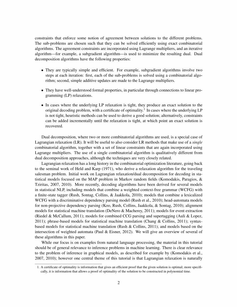
Figure 1: An example parse tree.

4. An Example: Integration of a Parser and a Finite-State Tagger

We next describe a dual decomposition algorithm for decoding under a model that combines aweighted context-free grammar and a finite-state tagger. The classical approach for this problemis to use a dynamic programming algorithm, based on the construction of Bar-Hillel, Perles, andShamir (1964) for the intersection of a context-free language and a finite-state language. The dualdecomposition algorithm has advantages over exhaustive dynamic programming, in terms of bothefficiency and simplicity. We will use this dual decomposition algorithm as a running examplethroughout this tutorial.

We first give a formal definition of the problem, describe motivation for the problem, and de-scribe the classical dynamic programming approach. We then describe the dual decompositionalgorithm.

4.1 Definition of the Problem

Consider the problem of mapping an input sentence x to a parse tree y. Define Y to be the set of allparse trees for x. The parsing problem is to find

y⇤ = argmaxy2Y

h(y) (8)

where h(y) is the score for any parse tree y 2 Y .We consider the case where h(y) is the sum of two model scores: first, the score for y under a

weighted context-free grammar; and second, the score for the part-of-speech (POS) sequence in yunder a finite-state part-of-speech tagging model. More formally, we define h(y) to be

h(y) = f(y) + g(l(y)) (9)

where the functions f , g, and l are defined as follows:

1. f(y) is the score for y under a weighted context-free grammar (WCFG). A WCFG consists ofa context-free grammar with a set of rules G, and a scoring function ✓ : G! R that assigns areal-valued score to each rule in G. The score for an entire parse tree is the sum of scores forthe rules it contains. As an example, consider the parse tree shown in figure 1; for this tree,

f(y) = ✓(S! NP VP) + ✓(NP! N) + ✓(N! United)+✓(VP! V NP) + . . .

9

We remain agnostic as to how the scores for individual context-free rules are defined. As oneexample, in a probabilistic context-free grammar, we would define ✓(↵ ! �) = log p(↵ !�|↵). As a second example, in a conditional random field (CRF) (Lafferty, McCallum, &Pereira, 2001) we would define ✓(↵ ! �) = w · �(↵ ! �) where w 2 Rq is a parametervector, and �(↵! �) 2 Rq is a feature vector representing the rule ↵! �.

2. l(y) is a function that maps a parse tree y to the sequence of part-of-speech tags in y. For theparse tree in figure 1, l(y) would be the sequence N V D A N.

3. g(z) is the score for the part-of-speech tag sequence z under a k’th-order finite-state taggingmodel. Under this model, if zi for i = 1 . . . n is the i’th tag in z, then

g(z) =nX

i=1

✓(i, zi�k, zi�k+1, . . . , zi)

where ✓(i, zi�k, zi�k+1, . . . , zi) is the score for the sub-sequence of tags zi�k, zi�k+1, . . . , zi

ending at position i in the sentence.3

We again remain agnostic as to how these ✓ terms are defined. As one example, g(z) mightbe the log-probability for z under a hidden Markov model, in which case

✓(i, zi�k . . . zi) = log p(zi|zi�k . . . zi�1) + log p(xi|zi)

where xi is the i’th word in the input sentence. As another example, under a CRF we wouldhave

✓(i, zi�k . . . zi) = w · �(x, i, zi�k . . . zi)

where w 2 Rq is a parameter vector, and �(x, i, zi�k . . . zi) is a feature-vector representationof the sub-sequence of tags zi�k . . . zi ending at position i in the sentence x.

The motivation for this problem is as follows. The scoring function h(y) = f(y) + g(l(y))combines information from both the parsing model and the tagging model. The two models capturefundamentally different types of information: in particular, the part-of-speech tagger captures in-formation about adjacent POS tags that will be missing under f(y). This information may improveboth parsing and tagging performance, in comparison to using f(y) alone.4

Under this definition of h(y), the conventional approach to finding y⇤ in Eq. 8 is to to constructa new context-free grammar that introduces sensitivity to surface bigrams (Bar-Hillel et al., 1964).Roughly speaking, in this approach (assuming a first-order tagging model) rules such as

S! NP VP

are replaced with rules such asSD,A ! NPD,N VPV,A (10)

3. We define zi for i 0 to be a special “start” POS symbol.4. We have assumed that it is sensible, in a theoretical and/or empirical sense, to take a sum of the scores f(y) and

g(l(y)). This might be the case, for example, if f(y) and g(z) are defined through structured prediction models (e.g.,conditional random fields), and their parameters are estimated jointly using discriminative methods. If f(y) and g(z)

are log probabilities under a PCFG and HMM respectively, then from a strict probabilistic sense it does not makesense to combine their scores in this way: however in practice this may work well; for example, this type of log-linearcombination of probabilistic models is widely used in approaches for statistical machine translation.

10

where each non-terminal (e.g., VP), is replaced with a non-terminal that tracks the first and last POStag under that non-terminal. For example, VPV,A represents a VP that dominates a sub-tree whosefirst POS tag is V, and whose last POS tag is A. The weights on the new rules include context-freeweights from f(y), and bigram scores from g(z). A dynamic programming parsing algorithm—forexample the CKY algorithm—can then be used to find the highest scoring structure under the newgrammar.

This approach is guaranteed to give an exact solution to the problem in Eq. 8; however it is oftenvery inefficient. We have greatly increased the size of the grammar by introducing the refined non-terminals, and this leads to significantly slower parsing performance. As one example, consider thecase where the underlying grammar is a CFG in Chomsky-normal form, with G non-terminals, andwhere we use a 2nd order (trigram) tagging model, with T possible part-of-speech tags. Parsing withthe grammar alone would take O(G3n3) time, for example using the CKY algorithm. In contrast,the construction of Bar-Hillel et al. (1964) results in an algorithm with a run time of O(G3T 6n3).The addition of the tagging model leads to a multiplicative factor of T 6 in the runtime of the parser,which is a very significant decrease in efficiency (it is not uncommon for T to take values of say 5or 50, giving values for T 6 larger than 15, 000 or 15 million).

In contrast, the dual decomposition algorithm which we describe next takes O(k(G3n3 +T 3n))time for this problem, where k is the number of iterations required for convergence; in experiments,k is often a small number. This is a very significant improvement in runtime over the Bar-Hillelet al. (1964) method.

4.2 The dual decomposition algorithm.

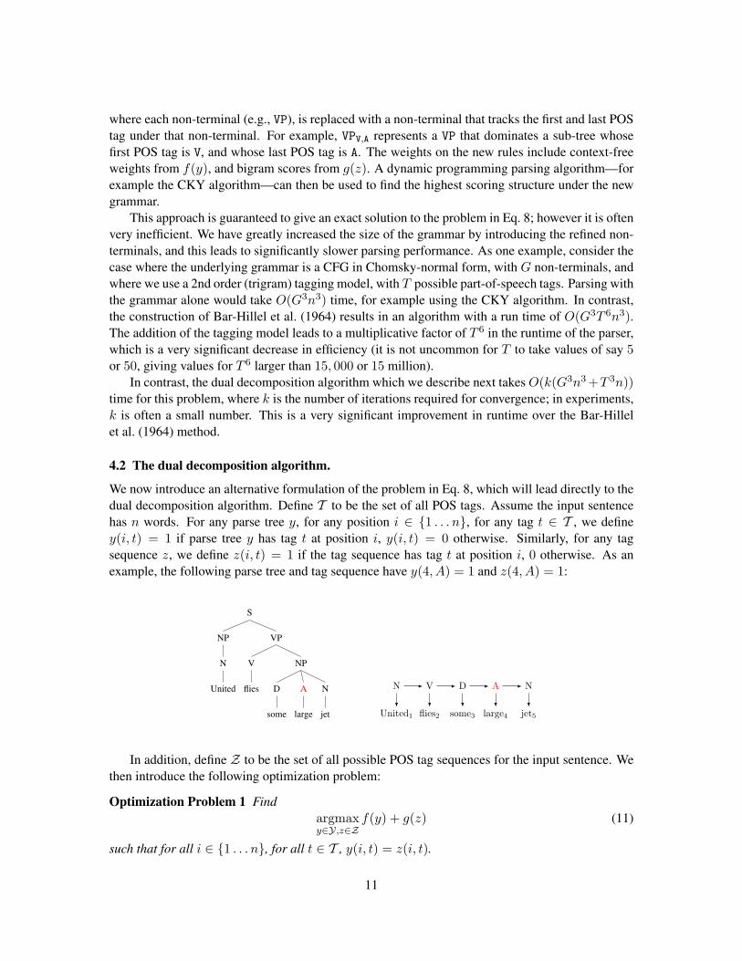
We now introduce an alternative formulation of the problem in Eq. 8, which will lead directly to thedual decomposition algorithm. Define T to be the set of all POS tags. Assume the input sentencehas n words. For any parse tree y, for any position i 2 {1 . . . n}, for any tag t 2 T , we definey(i, t) = 1 if parse tree y has tag t at position i, y(i, t) = 0 otherwise. Similarly, for any tagsequence z, we define z(i, t) = 1 if the tag sequence has tag t at position i, 0 otherwise. As anexample, the following parse tree and tag sequence have y(4, A) = 1 and z(4, A) = 1:

S

NP

N

United

VP

V

flies

NP

D

some

A

large

N

jet United1 flies2 some3 large4 jet5

N V D A N

In addition, define Z to be the set of all possible POS tag sequences for the input sentence. Wethen introduce the following optimization problem:

Optimization Problem 1 Findargmaxy2Y,z2Z

f(y) + g(z) (11)

such that for all i 2 {1 . . . n}, for all t 2 T , y(i, t) = z(i, t).

11

Thus we now find the best pair of structures y and z such that they share the same POS sequence.We define (y⇤, z⇤) to be the pair of structures that achieve the argmax in this problem. The crucialclaim, which is easily verified, is that y⇤ is also the argmax to the problem in Eq. 8. In this sense,solving the new problem immediately leads to a solution to our original problem.

We then make the following two assumptions. Whether these assumptions are satisfied willdepend on the definitions of Y and f(y) (for assumption 1) and on the definitions of Z and g(z)(for assumption 2). The assumptions hold when f(y) is a WCFG and g(z) is a finite-state tagger,but more generally they may hold for other parsing and tagging models.

Assumption 1 Assume that we introduce variables u(i, t) 2 R for i 2 {1 . . . n}, and t 2 T . Weassume that for any value of these variables, we can find

argmaxy2Y

0

@f(y) +X

i,t

u(i, t)y(i, t)

1

A

efficiently.

An example. Consider a WCFG where the grammar is in Chomsky normal form. The scoringfunction is defined as

f(y) =X

X!Y Z

c(y,X ! Y Z)✓(X ! Y Z) +X

i,t

y(i, t)✓(t! wi)

where we write c(y, X ! Y Z) to denote the number of times that rule X ! Y Z is seen in theparse tree y, and as before y(i, t) = 1 if word i has POS t, 0 otherwise (note that y(i, t) = 1 impliesthat the rule t ! wi is used in the parse tree). The highest scoring parse tree under f(y) can befound efficiently, for example using the CKY parsing algorithm. We then have

argmaxy2Y

0

@f(y) +X

i,t

u(i, t)y(i, t)

1

A =

argmaxy2Y

0

@X

X!Y Z

c(y, X ! Y Z)✓(X ! Y Z) +X

i,t

y(i, t)(✓(t! wi) + u(i, t))

1

A

This argmax can again be found easily using the CKY algorithm, where the scores ✓(t ! wi) aresimply replaced by new scores defined as ✓0(t! wi) = ✓(t! wi) + u(i, t).

Assumption 2 Assume that we introduce variables u(i, t) 2 R for i 2 {1 . . . n}, and t 2 T . Weassume that for any value of these variables, we can find

argmaxz2Z

0

@g(z)�X

i,t

u(i, t)z(i, t)

1

A

efficiently.

12

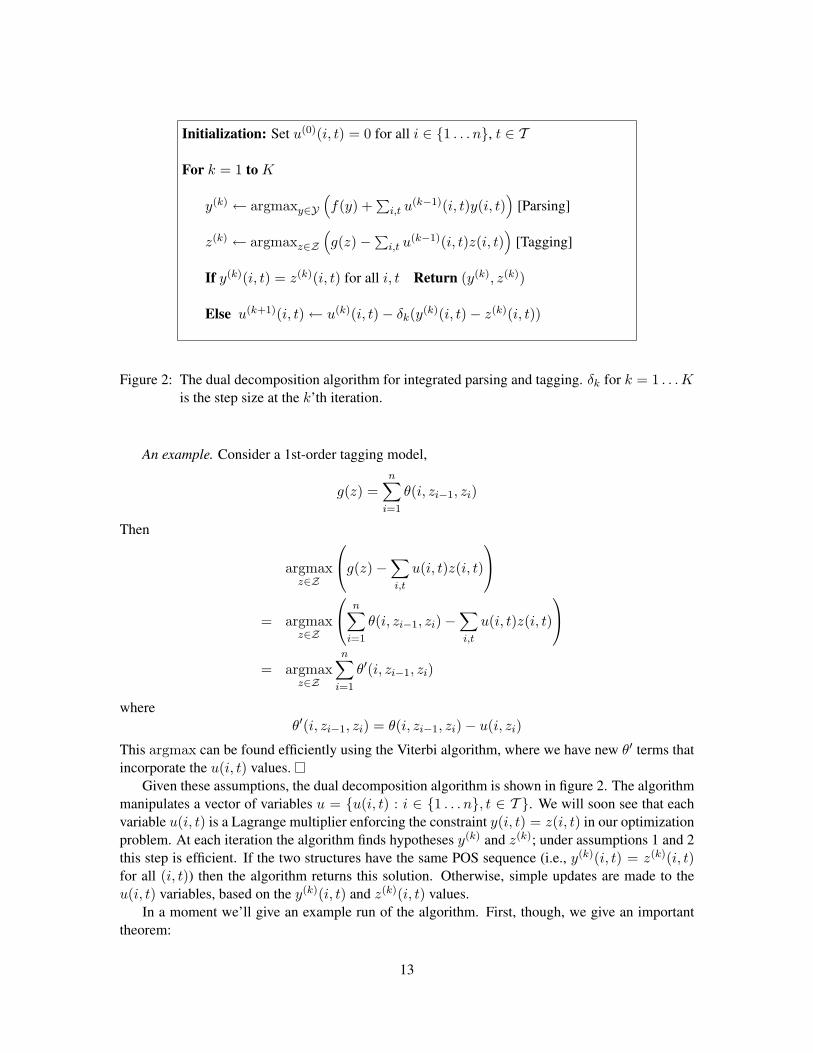
Initialization: Set u(0)(i, t) = 0 for all i 2 {1 . . . n}, t 2 T

For k = 1 to K

y(k) argmaxy2Y

⇣f(y) +

Pi,t u(k�1)(i, t)y(i, t)

⌘[Parsing]

z(k) argmaxz2Z

⇣g(z)�

Pi,t u(k�1)(i, t)z(i, t)

⌘[Tagging]

If y(k)(i, t) = z(k)(i, t) for all i, t Return (y(k), z(k))

Else u(k+1)(i, t) u(k)(i, t)� �k(y(k)(i, t)� z(k)(i, t))

Figure 2: The dual decomposition algorithm for integrated parsing and tagging. �k for k = 1 . . . Kis the step size at the k’th iteration.

An example. Consider a 1st-order tagging model,

g(z) =nX

i=1

✓(i, zi�1, zi)

Then

argmaxz2Z

0

@g(z)�X

i,t

u(i, t)z(i, t)

1

A

= argmaxz2Z

0

@nX

i=1

✓(i, zi�1, zi)�X

i,t

u(i, t)z(i, t)

1

A

= argmaxz2Z

nX

i=1

✓0(i, zi�1, zi)

where✓0(i, zi�1, zi) = ✓(i, zi�1, zi)� u(i, zi)

This argmax can be found efficiently using the Viterbi algorithm, where we have new ✓0 terms thatincorporate the u(i, t) values.

Given these assumptions, the dual decomposition algorithm is shown in figure 2. The algorithmmanipulates a vector of variables u = {u(i, t) : i 2 {1 . . . n}, t 2 T }. We will soon see that eachvariable u(i, t) is a Lagrange multiplier enforcing the constraint y(i, t) = z(i, t) in our optimizationproblem. At each iteration the algorithm finds hypotheses y(k) and z(k); under assumptions 1 and 2this step is efficient. If the two structures have the same POS sequence (i.e., y(k)(i, t) = z(k)(i, t)for all (i, t)) then the algorithm returns this solution. Otherwise, simple updates are made to theu(i, t) variables, based on the y(k)(i, t) and z(k)(i, t) values.

In a moment we’ll give an example run of the algorithm. First, though, we give an importanttheorem:

13

Theorem 2 If at any iteration of the algorithm in figure 2 we have y(k)(i, t) = z(k)(i, t) for all(i, t), then (y(k), z(k)) is a solution to optimization problem 1.

Thus if we do reach agreement between y(k) and z(k), then we are guaranteed to have an optimalsolution to the original problem. Later in this tutorial we will give empirical results for various NLPproblems showing how often, and how quickly, we reach agreement. We will also describe thetheory underlying convergence; theory underlying cases where the algorithm doesn’t converge; andmethods that can be used to “tighten” the algorithm with the goal of achieving convergence.

Next, consider the efficiency of the algorithm. To be concrete, again consider the case wheref(y) is defined through a weighted CFG, and g(z) is defined through a finite-state tagger. Eachiteration of the algorithm requires decoding under each of these two models. If the number ofiterations k is relatively small, the algorithm can be much more efficient than using the constructionfrom Bar-Hillel et al. (1964). As discussed before, assuming a context-free grammar in Chomskynormal form, and a trigram tagger with T tags, the CKY parsing algorithm takes O(G3n3) time,and the Viterbi algorithm for tagging takes O(T 3n) time. Thus the total running time for the dualdecomposition algorithm is O(k(G3n3 + T 3n)) where k is the number of iterations required forconvergence. In contrast, the construction of Bar-Hillel et al. (1964) results in an algorithm withrunning time of O(G3T 6n3). The dual decomposition algorithm results in an additive cost forincorporating a tagger (a T 3n term is added into the run time), whereas the construction of Bar-Hillel et al. (1964) results in a much more expensive multiplicative cost (a T 6 term is multipliedinto the run time). (Smith and Eisner (2008) make a similar observation about additive versusmultiplicative costs in the context of belief propagation algorithms for dependency parsing.)

4.3 Relationship of the Approach to Section 3

It is easily verified that the approach we have described is an instance of the dual decompositionframework described in section 3.2. The set Y is the set of all parses for the input sentence; the setZ is the set of all POS sequences for the input sentence. Each parse tree y 2 Rd is represented asa vector such that f(y) = y · ✓(1) for some ✓(1) 2 Rd: there are a number of ways of representingparse trees as vectors, see Rush et al. (2010) for one example. Similarly, each tag sequence z 2 Rd0

is represented as a vector such that g(z) = z · ✓(2) for some ✓(2) 2 Rd0 . The constraints

y(i, t) = z(i, t)

for all (i, t) can be encoded through linear constraints

Ay + Cz = b

for suitable choices of A, C, and b, assuming that the vectors y and z include components y(i, t)and z(i, t) respectively.

4.4 An Example Run of the Algorithm

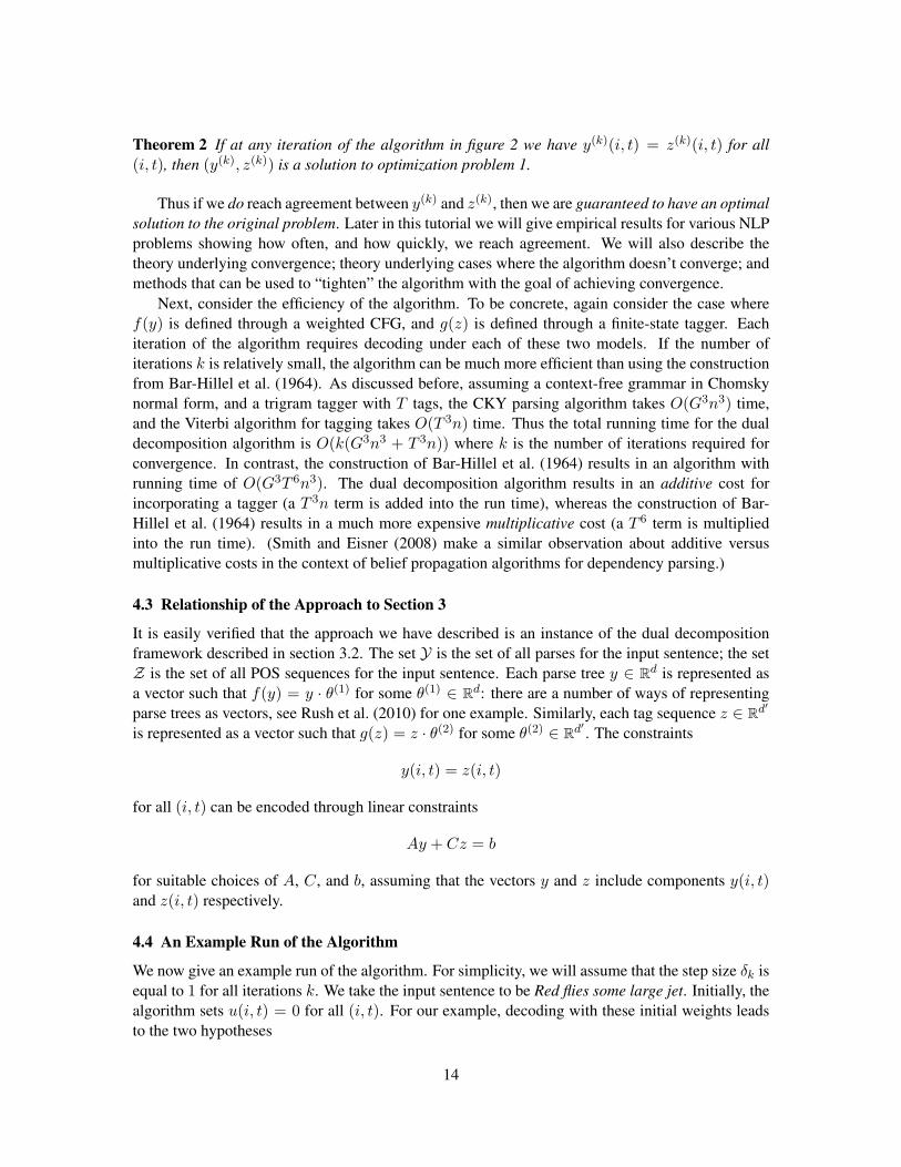
We now give an example run of the algorithm. For simplicity, we will assume that the step size �k isequal to 1 for all iterations k. We take the input sentence to be Red flies some large jet. Initially, thealgorithm sets u(i, t) = 0 for all (i, t). For our example, decoding with these initial weights leadsto the two hypotheses

14

S

NP

A

Red

N

flies

D

some

A

large

VP

V

jet Red1 flies2 some3 large4 jet5

N V D A N

These two structures have different POS tags at three positions, highlighted in red; thus the twostructures do not agree. We then update the u(i, t) variables based on these differences, giving newvalues as follows:

u(1, A) = u(2, N) = u(5, V ) = �1

u(1, N) = u(2, V ) = u(5, N) = 1

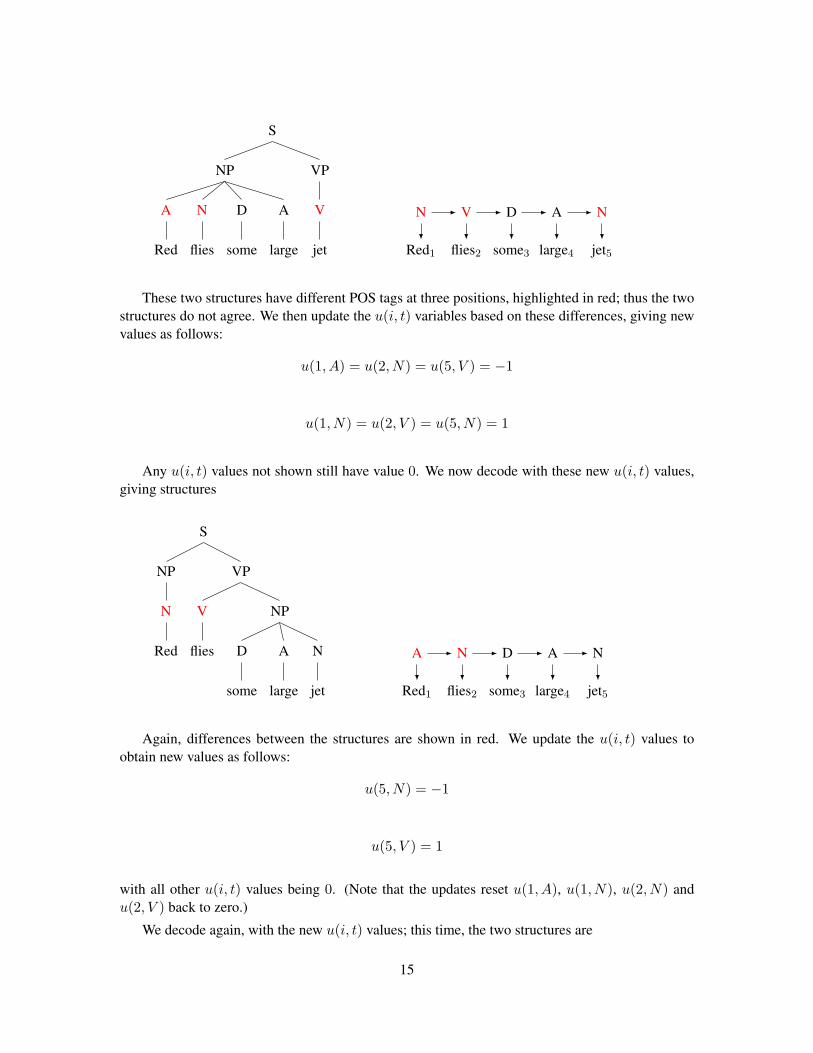
Any u(i, t) values not shown still have value 0. We now decode with these new u(i, t) values,giving structures

S

NP

N

Red

VP

V

flies

NP

D

some

A

large

N

jet Red1 flies2 some3 large4 jet5

A N D A N

Again, differences between the structures are shown in red. We update the u(i, t) values toobtain new values as follows:

u(5, N) = �1

u(5, V ) = 1

with all other u(i, t) values being 0. (Note that the updates reset u(1, A), u(1, N), u(2, N) andu(2, V ) back to zero.)

We decode again, with the new u(i, t) values; this time, the two structures are

15

0

20

40

60

80

100

<=1<=2

<=3<=4

<=10<=20

<=50

% e

xam

ples

con

verg

ed

number of iterations

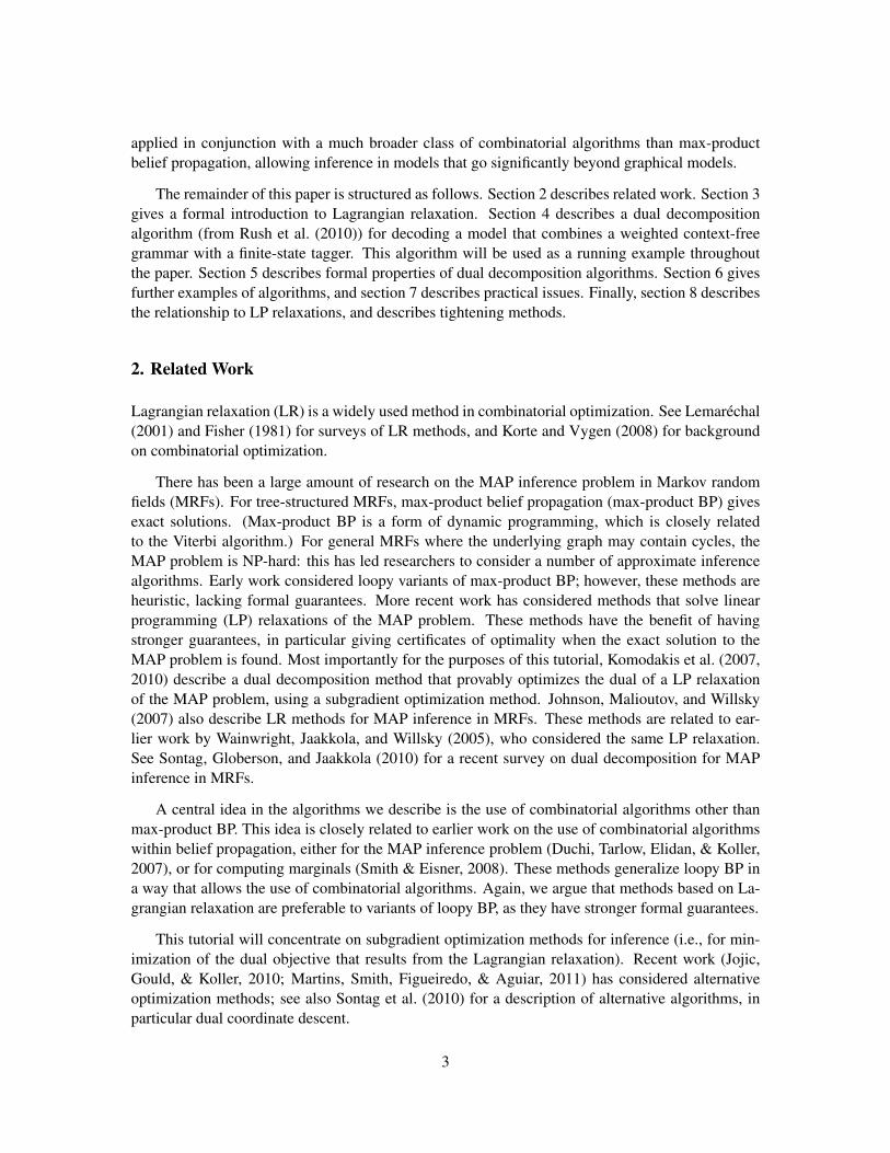
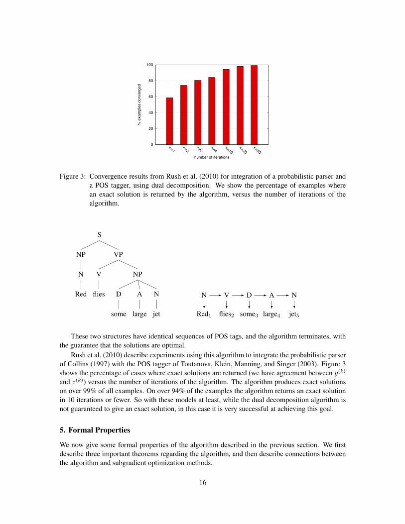
Figure 3: Convergence results from Rush et al. (2010) for integration of a probabilistic parser anda POS tagger, using dual decomposition. We show the percentage of examples wherean exact solution is returned by the algorithm, versus the number of iterations of thealgorithm.

S

NP

N

Red

VP

V

flies

NP

D

some

A

large

N

jet Red1 flies2 some3 large4 jet5

N V D A N

These two structures have identical sequences of POS tags, and the algorithm terminates, withthe guarantee that the solutions are optimal.

Rush et al. (2010) describe experiments using this algorithm to integrate the probabilistic parserof Collins (1997) with the POS tagger of Toutanova, Klein, Manning, and Singer (2003). Figure 3shows the percentage of cases where exact solutions are returned (we have agreement between y(k)

and z(k)) versus the number of iterations of the algorithm. The algorithm produces exact solutionson over 99% of all examples. On over 94% of the examples the algorithm returns an exact solutionin 10 iterations or fewer. So with these models at least, while the dual decomposition algorithm isnot guaranteed to give an exact solution, in this case it is very successful at achieving this goal.

5. Formal Properties

We now give some formal properties of the algorithm described in the previous section. We firstdescribe three important theorems regarding the algorithm, and then describe connections betweenthe algorithm and subgradient optimization methods.

16

5.1 Three Theorems

Recall that the problem we are attempting to solve (optimization problem 1) is

argmaxy2Y,z2Z

f(y) + g(z)

such that for all i = 1 . . . n, t 2 T ,y(i, t) = z(i, t)

The first step will be to introduce the Lagrangian for this problem. We introduce a Lagrangemultiplier u(i, t) for each equality constraint y(i, t) = z(i, t): we write u = {u(i, t) : i 2{1 . . . n}, t 2 T } to denote the vector of Lagrange mulipliers. Each Lagrange multiplier can takeany positive or negative value. The Lagrangian is

L(u, y, z) = f(y) + g(z) +X

i,t

u(i, t) (y(i, t)� z(i, t)) (12)

Note that by grouping the terms that depend on y and z, we can rewrite the Lagrangian as

L(u, y, z) =

0

@f(y) +X

i,t

u(i, t)y(i, t)

1

A+

0

@g(z)�X

i,t

u(i, t)z(i, t)

1

A

Having defined the Lagrangian, the dual objective is

L(u) = maxy2Y,z2Z

L(u, y, z)

= maxy2Y

0

@f(y) +X

i,t

u(i, t)y(i, t)

1

A+ maxz2Z

0

@g(z)�X

i,t

u(i, t)z(i, t)

1

A

Under assumptions 1 and 2 described above, the dual value L(u) for any value of u can be calculatedefficiently: we simply compute the two max’s, and sum them. Thus the dual decomposes in a veryconvenient way into two efficiently solvable sub-problems.

Finally, the dual problem is to minimize the dual objective, that is, to find

minu

L(u)

We will see shortly that the algorithm in figure 2 is a subgradient algorithm for minimizing the dualobjective.

Define (y⇤, z⇤) to be the optimal solution to optimization problem 1. The first theorem is asfollows:

Theorem 3 For any value of u,L(u) � f(y⇤) + g(z⇤)

Hence L(u) provides an upper bound on the score of the optimal solution. The proof is simple:

17

Proof:

L(u) = maxy2Y,z2Z

L(u, y, z) (13)

� maxy2Y,z2Z:y=z

L(u, y, z) (14)

= maxy2Y,z2Z:y=z

f(y) + g(z) (15)

= f(y⇤) + g(z⇤) (16)

Here we use the shorthand y = z to state that y(i, t) = z(i, t) for all (i, t). Eq. 14 follows becauseby adding the constraints y = z, we are optimizing over a smaller set of (y, z) pairs, and hence themax cannot increase. Eq. 15 follows because if y = z, we have

X

i,t

u(i, t) (y(i, t)� z(i, t)) = 0

and hence L(u, y, z) = f(y) + g(z). Finally, Eq. 16 follows through the definition of y⇤ and z⇤.Note that obtaining an upper bound on f(y⇤) + g(z⇤) (providing that it is relatively tight) can

be a useful goal in itself. First, upper bounds of this form can be used as admissible heuristics forsearch methods such as A* or branch-and-bound algorithms. Second, if we have some method thatgenerates a potential solution (y, z), we immediately obtain an upper bound on how far this solutionis from being optimal, because

(f(y⇤) + g(z⇤))� (f(y) + g(z)) L(u)� (f(y) + g(z))

Hence if L(u)� (f(y) + g(z)) is small, then (f(y⇤) + g(z⇤))� (f(y) + g(z)) must be small. Seesection 7 for more discussion.

Our second theorem states that the algorithm in figure 2 successfully converges to minu L(u).Hence the algorithm successfully converges to the tightest possible upper bound given by the dual.The theorem is as follows:

Theorem 4 Consider the algorithm in figure 2. For any sequence �1, �2, �3, . . . such that �k > 0for all k � 1, and

limk!1

�k = 0 and1X

k=1

�k =1,

we havelim

k!1L(uk) = min

uL(u)

Proof: See Shor (1985). See also appendix A.3.Our algorithm is actually a subgradient method for minimizing L(u): we return to this point in

section 5.2. For now though, the important point is that our algorithm successfully minimizes L(u).Our final theorem states that if we ever reach agreement during the algorithm in figure 2, we are

guaranteed to have the optimal solution. We first need the following definitions:

18

Definition 1 For any value of u, define

y(u) = argmaxy2Y

0

@f(y) +X

i,t

u(i, t)y(i, t)

1

A

and

z(u) = argmaxz2Z

0

@g(z)�X

i,t

u(i, t)z(i, t)

1

A

The theorem is then:

Theorem 5 If 9u such thaty(u)(i, t) = z(u)(i, t)

for all i, t, thenf(y(u)) + g(z(u)) = f(y⇤) + g(z⇤)

i.e., (y(u), z(u)) is optimal.

Proof: We have, by the definitions of y(u) and z(u),

L(u) = f(y(u)) + g(z(u)) +X

i,t

u(i, t)(y(u)(i, t)� z(u)(i, t))

= f(y(u)) + g(z(u))

where the second equality follows because y(u)(i, t) = z(u)(i, t) for all (i, t). But L(u) � f(y⇤) +g(z⇤) for all values of u, hence

f(y(u)) + g(z(u)) � f(y⇤) + g(z⇤)

Because y⇤ and z⇤ are optimal, we also have

f(y(u)) + g(z(u)) f(y⇤) + g(z⇤)

hence we must havef(y(u)) + g(z(u)) = f(y⇤) + g(z⇤)

Theorems 4 and 5 refer to quite different notions of convergence of the dual decompositionalgorithm. For the remainder of this tutorial, to avoid confusion, we will explicitly use the followingterms:

• d-convergence (short for “dual convergence”) will be used to refer to convergence of the dualdecomposition algorithm to the minimum dual value: that is, the property that limk!1 L(u(k)) =minu L(u). By theorem 4, assuming appropriate step sizes in the algorithm, we always haved-convergence.

• e-convergence (short for “exact convergence”) refers to convergence of the dual decompo-sition algorithm to a point where y(i, t) = z(i, t) for all (i, t). By theorem 5, if the dualdecomposition algorithm e-converges, then it is guaranteed to have provided the optimal so-lution. However, the algorithm is not guaranteed to e-converge.

19

5.2 Subgradients

The proof of d-convergence, as defined in theorem 4, relies on the fact that the algorithm in figure 2is a subgradient algorithm for minimizing the dual objective L(u). Subgradient algorithms are ageneralization of gradient-descent methods; they can be used to minimize convex functions that arenon-differentiable. This section describes how the algorithm in figure 2 is derived as a subgradientalgorithm.

Recall that L(u) is defined as follows:

L(u) = maxy2Y,z2Z

L(u, y, z)

= maxy2Y

0

@f(y) +X

i,t

u(i, t)y(i, t)

1

A+ maxz2Z

0

@g(z)�X

i,t

u(i, t)z(i, t)

1

A

and that our goal is to find minu L(u).First, we note that L(u) has the following properties:

• L(u) is a convex function. That is, for any u(1) 2 Rd, u(2) 2 Rd, � 2 [0, 1],

L(�u(1) + (1� �)u(2)) �L(u(1)) + (1� �)L(u(2))

(The proof is simple: see appendix A.1.)

• L(u) is not differentiable. In fact, it is easily shown that it is a piecewise linear function.

The fact that L(u) is not differentiable means that we cannot use a gradient descent method tominimize it. However, because it is nevertheless a convex function, we can instead use a subgradientalgorithm. The definition of a subgradient is as follows:

Definition 2 (Subgradient) A subgradient of a convex function L : Rd ! R at u is a vector �(u)

such that for all v 2 Rd,L(v) � L(u) + �(u) · (v � u)

The subgradient �(u) is a tangent at the point u that gives a lower bound to L(u): in this senseit is similar to the gradient for a convex but differentiable function.5 The key idea in subgradientmethods is to use subgradients in the same way that we would use gradients in gradient descentmethods. That is, we use updates of the form

u0 = u� ��(u)

where u is the current point in the search, �(u) is a subgradient at this point, � > 0 is a step size, andu0 is the new point in the search. Under suitable conditions on the stepsizes �, these updates willsuccessfully converge to the minimum of L(u).

So how do we calculate the subgradient for L(u)? It turns out that it has a very convenientform. As before (see definition 1), define y(u) and z(u) to be the argmax’s for the two maximizationproblems in L(u). If we define the vector �(u) as

�(u)(i, t) = y(u)(i, t)� z(u)(i, t)

5. It should be noted, however, that for a given point u, there may be more than one subgradient: this will occur, forexample, for a piecewise linear function at points where the gradient is not defined.

20

S(flies)

NP(United)

N

United

VP(flies)

V

flies

NP(jet)

D

some

A

large

N

jet *0 United1 flies2 some3 large4 jet5

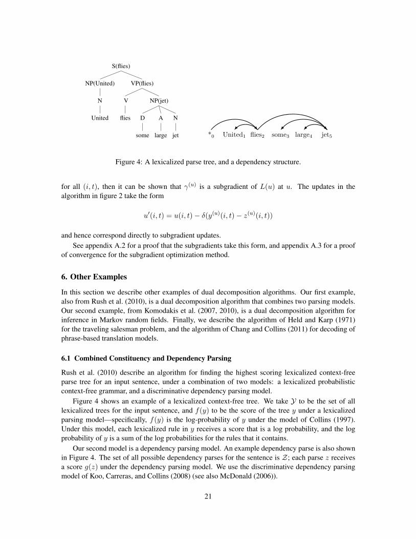
Figure 4: A lexicalized parse tree, and a dependency structure.

for all (i, t), then it can be shown that �(u) is a subgradient of L(u) at u. The updates in thealgorithm in figure 2 take the form

u0(i, t) = u(i, t)� �(y(u)(i, t)� z(u)(i, t))

and hence correspond directly to subgradient updates.See appendix A.2 for a proof that the subgradients take this form, and appendix A.3 for a proof

of convergence for the subgradient optimization method.

6. Other Examples

In this section we describe other examples of dual decomposition algorithms. Our first example,also from Rush et al. (2010), is a dual decomposition algorithm that combines two parsing models.Our second example, from Komodakis et al. (2007, 2010), is a dual decomposition algorithm forinference in Markov random fields. Finally, we describe the algorithm of Held and Karp (1971)for the traveling salesman problem, and the algorithm of Chang and Collins (2011) for decoding ofphrase-based translation models.

6.1 Combined Constituency and Dependency Parsing

Rush et al. (2010) describe an algorithm for finding the highest scoring lexicalized context-freeparse tree for an input sentence, under a combination of two models: a lexicalized probabilisticcontext-free grammar, and a discriminative dependency parsing model.

Figure 4 shows an example of a lexicalized context-free tree. We take Y to be the set of alllexicalized trees for the input sentence, and f(y) to be the score of the tree y under a lexicalizedparsing model—specifically, f(y) is the log-probability of y under the model of Collins (1997).Under this model, each lexicalized rule in y receives a score that is a log probability, and the logprobability of y is a sum of the log probabilities for the rules that it contains.

Our second model is a dependency parsing model. An example dependency parse is also shownin Figure 4. The set of all possible dependency parses for the sentence is Z; each parse z receivesa score g(z) under the dependency parsing model. We use the discriminative dependency parsingmodel of Koo, Carreras, and Collins (2008) (see also McDonald (2006)).

21

0

20

40

60

80

100

<=1<=2

<=3<=4

<=10<=20

<=50

% e

xam

ples

con

verg

ed

number of iterations

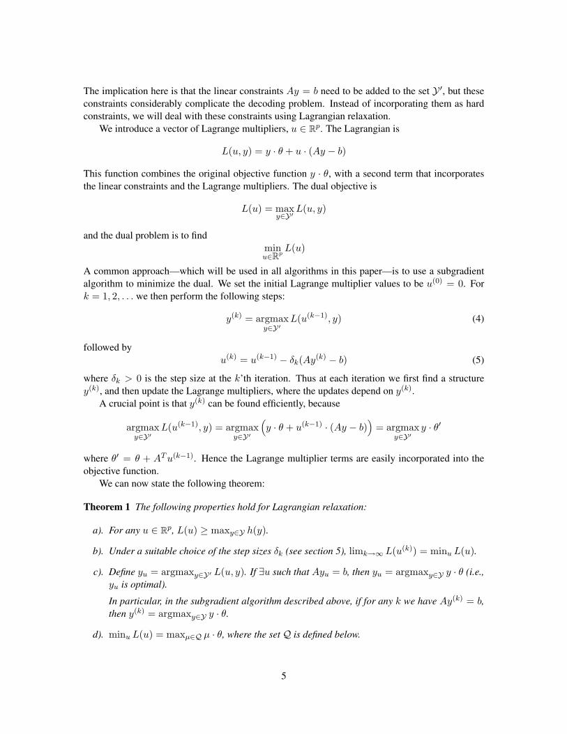
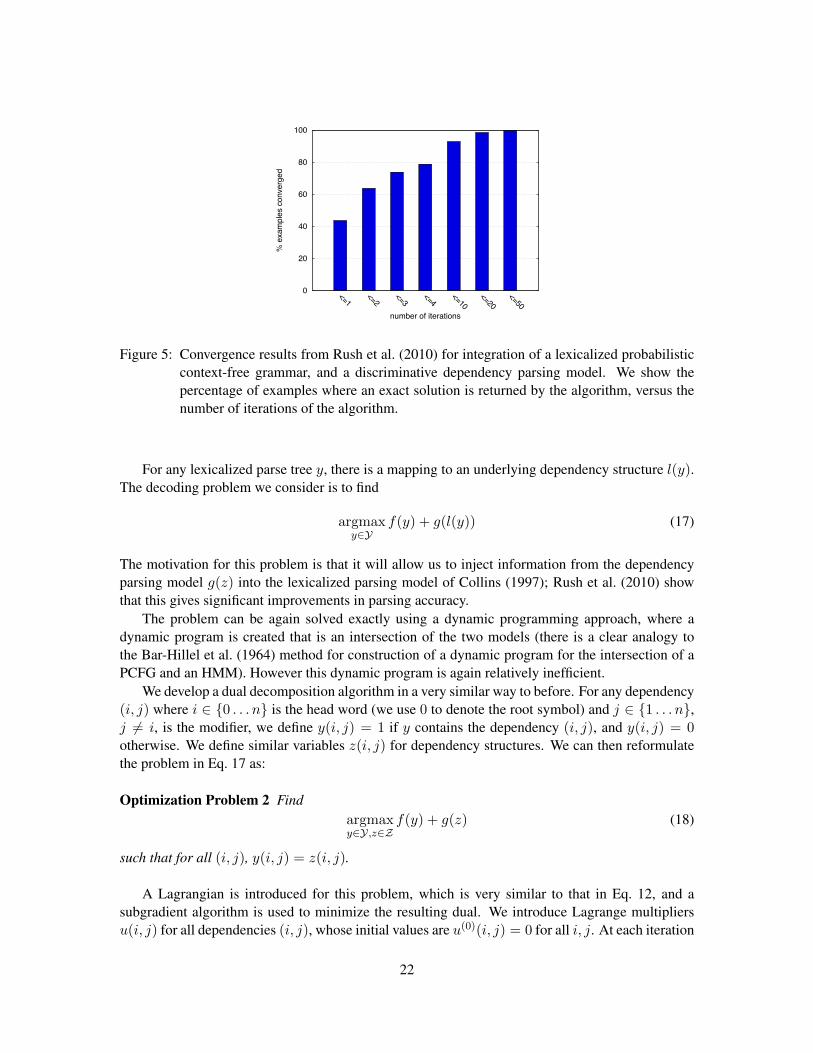
Figure 5: Convergence results from Rush et al. (2010) for integration of a lexicalized probabilisticcontext-free grammar, and a discriminative dependency parsing model. We show thepercentage of examples where an exact solution is returned by the algorithm, versus thenumber of iterations of the algorithm.

For any lexicalized parse tree y, there is a mapping to an underlying dependency structure l(y).The decoding problem we consider is to find

argmaxy2Y

f(y) + g(l(y)) (17)

The motivation for this problem is that it will allow us to inject information from the dependencyparsing model g(z) into the lexicalized parsing model of Collins (1997); Rush et al. (2010) showthat this gives significant improvements in parsing accuracy.

The problem can be again solved exactly using a dynamic programming approach, where adynamic program is created that is an intersection of the two models (there is a clear analogy tothe Bar-Hillel et al. (1964) method for construction of a dynamic program for the intersection of aPCFG and an HMM). However this dynamic program is again relatively inefficient.

We develop a dual decomposition algorithm in a very similar way to before. For any dependency(i, j) where i 2 {0 . . . n} is the head word (we use 0 to denote the root symbol) and j 2 {1 . . . n},j 6= i, is the modifier, we define y(i, j) = 1 if y contains the dependency (i, j), and y(i, j) = 0otherwise. We define similar variables z(i, j) for dependency structures. We can then reformulatethe problem in Eq. 17 as:

Optimization Problem 2 Findargmaxy2Y,z2Z

f(y) + g(z) (18)

such that for all (i, j), y(i, j) = z(i, j).

A Lagrangian is introduced for this problem, which is very similar to that in Eq. 12, and asubgradient algorithm is used to minimize the resulting dual. We introduce Lagrange multipliersu(i, j) for all dependencies (i, j), whose initial values are u(0)(i, j) = 0 for all i, j. At each iteration

22

of the algorithm we find

y(k) = argmaxy2Y

0

@f(y) +X

i,j

u(k�1)(i, j)y(i, j)

1

A

using a dynamic programming algorithm for lexicalized context-free parsing (a trivial modificationof the original algorithm for finding argmaxy f(y)). In addition we find

z(k) = argmaxz2Z

0

@g(z)�X

i,j

u(k�1)(i, j)z(i, j)

1

A

using a dynamic programming algorithm for dependency parsing (again, this requires a trivial mod-ification to an existing algorithm). If y(k)(i, j) = z(k)(i, j) for all (i, j) then the algorithm hase-converged, and we are guaranteed to have a solution to optimization problem 2. Otherwise, weperform subgradient updates

u(k)(i, j) = u(k�1)(i, j)� �k(y(k)(i, j)� z(k)(i, j))

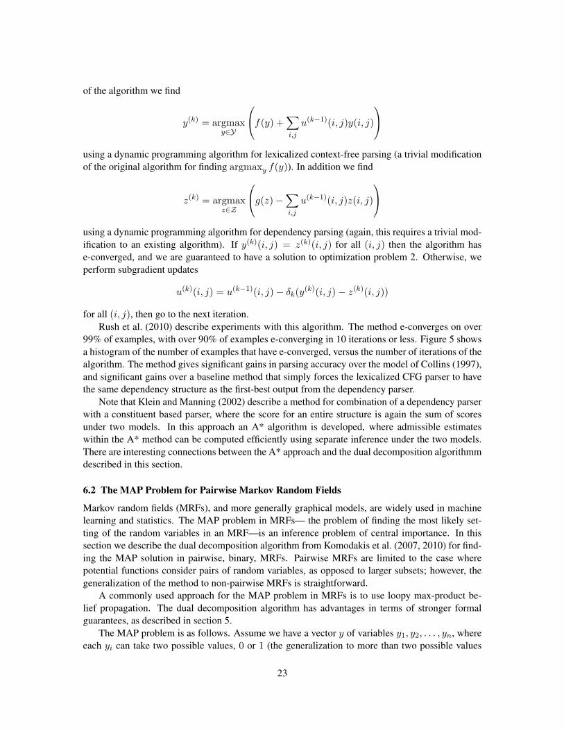
for all (i, j), then go to the next iteration.Rush et al. (2010) describe experiments with this algorithm. The method e-converges on over

99% of examples, with over 90% of examples e-converging in 10 iterations or less. Figure 5 showsa histogram of the number of examples that have e-converged, versus the number of iterations of thealgorithm. The method gives significant gains in parsing accuracy over the model of Collins (1997),and significant gains over a baseline method that simply forces the lexicalized CFG parser to havethe same dependency structure as the first-best output from the dependency parser.

Note that Klein and Manning (2002) describe a method for combination of a dependency parserwith a constituent based parser, where the score for an entire structure is again the sum of scoresunder two models. In this approach an A* algorithm is developed, where admissible estimateswithin the A* method can be computed efficiently using separate inference under the two models.There are interesting connections between the A* approach and the dual decomposition algorithmmdescribed in this section.

6.2 The MAP Problem for Pairwise Markov Random Fields

Markov random fields (MRFs), and more generally graphical models, are widely used in machinelearning and statistics. The MAP problem in MRFs— the problem of finding the most likely set-ting of the random variables in an MRF—is an inference problem of central importance. In thissection we describe the dual decomposition algorithm from Komodakis et al. (2007, 2010) for find-ing the MAP solution in pairwise, binary, MRFs. Pairwise MRFs are limited to the case wherepotential functions consider pairs of random variables, as opposed to larger subsets; however, thegeneralization of the method to non-pairwise MRFs is straightforward.

A commonly used approach for the MAP problem in MRFs is to use loopy max-product be-lief propagation. The dual decomposition algorithm has advantages in terms of stronger formalguarantees, as described in section 5.

The MAP problem is as follows. Assume we have a vector y of variables y1, y2, . . . , yn, whereeach yi can take two possible values, 0 or 1 (the generalization to more than two possible values

23

for each variable is straightforward). There are 2n possible settings of these n variables. An MRFassumes an underlying undirected graph (V,E), where V = {1 . . . n} is the set of vertices in thegraph, and E is a set of edges. The MAP problem is then to find

argmaxy2{0,1}n

h(y) (19)

whereh(y) =

X

{i,j}2E

✓i,j(yi, yj)

Here each ✓i,j(yi, yj) is a local potential associated with the edge {i, j} 2 E, which returns a realvalue (positive or negative) for each of the four possible settings of (yi, yj).

If the underlying graph E is a tree, the problem in Eq. 19 is easily solved using max-productbelief propagation, a form of dynamic programming. In contrast, for general graphs E, which maycontain loops, the problem is NP-hard. The key insight behind the dual decomposition algorithmwill be to decompose the graph E into m trees T1, T2, . . . , Tm. Inference over each tree can beperformed efficiently; we use Lagrange multipliers to enforce agreement between the inferenceresults for each tree. A subgradient algorithm is used, where at each iteration we first performinference over each of the trees T1, T2, . . . , Tm, and then update the Lagrange multipliers in caseswhere there are disagreements.

For simplicity, we describe the case where m = 2. Assume that the two trees are such thatT1 ⇢ E, T2 ⇢ E, and T1 [ T2 = E.6 Thus each of the trees contains a subset of the edges inE, but together the trees contain all edges in E. Assume that we define potential functions ✓

(1)i,j for

(i, j) 2 T1 and ✓(2)i,j for (i, j) 2 T2 such that

X

{i,j}2E

✓i,j(yi, yj) =X

{i,j}2T1

✓(1)i,j (yi, yj) +

X

{i,j}2T2

✓(2)i,j (yi, yj)

This is easy to do: for example, define

✓mi,j(yi, yj) =

✓i,j(yi, yj)#(i, j)

for m = 1, 2 where #(i, j) is 2 if the edge {i, j} appears in both trees, 1 otherwise.We can then define a new problem that is equivalent to the problem in Eq. 19:

Optimization Problem 3 Find

argmaxy2{0,1}n,z2{0,1}n

X

{i,j}2T1

✓(1)i,j (yi, yj) +

X

{i,j}2T2

✓(2)i,j (zi, zj)

such that yi = zi for i = 1 . . . n.

6. It may not always be possible to decompose a graph E into just 2 trees in this way. Komodakis et al. (2007, 2010)describe an algorithm for the general case of more than 2 trees.

24

Note the similarity to our previous optimization problems. Our goal is to find a pair of structures,y 2 {0, 1}n and z 2 {0, 1}n. The objective function can be written as

f(y) + g(z)

wheref(y) =

X

{i,j}2T1

✓(1)i,j (yi, yj)

andg(z) =

X

{i,j}2T2

✓(2)i,j (zi, zj)

We have a set of constraints, yi = zi for i = 1 . . . n, which enforce agreement between y and z.We then proceed as before—we define a Lagrangian with a Lagrange multiplier ui for each

constraint:

L(u, y, z) =X

{i,j}2T1

✓(1)i,j (yi, yj) +

X

{i,j}2T2

✓(2)i,j (zi, zj) +

nX

i=1

ui(yi � zi)

We then minimize the dualL(u) = max

y,zL(u, y, z)

using a subgradient algorithm. The algorithm is initialized with u(0)i = 0 for i = 1 . . . n. At each

iteration of the algorithm we find

y(k) = argmaxy2{0,1}n

0

@X

{i,j}2T1

✓(1)i,j (yi, yj) +

X

i

u(k�1)i yi

1

A

and

z(k) = argmaxz2{0,1}n

0

@X

{i,j}2T2

✓(2)i,j (zi, zj)�

X

i

u(k�1)i zi

1

A

These steps can be achieved efficiently, because T1 and T2 are trees, hence max-product belief prop-agation produces an exact answer. (The Lagrangian terms

Pi u

(k�1)i yi and

Pi u

(k�1)i zi are easily

incorporated.) If y(k)i = z

(k)i for all i then the algorithm has e-converged, and we are guaranteed to

have a solution to optimization problem 3. Otherwise, we perform subgradient updates of the form

u(k)i = u

(k�1)i � �k(y

(k)i � z

(k)i )

for i = {1 . . . n}, then go to the next iteration. Intuitively, these updates will bias the two inferenceproblems towards agreement with each other.

Komodakis et al. (2007, 2010) show excellent experimental results for the method. The algo-rithm has some parallels to max-product belief propagation, where the ui values can be interpretedas “messages” being passed between sub-problems.

25

1

2

3

4

5

6

7

1

2

3

4

5

6

7

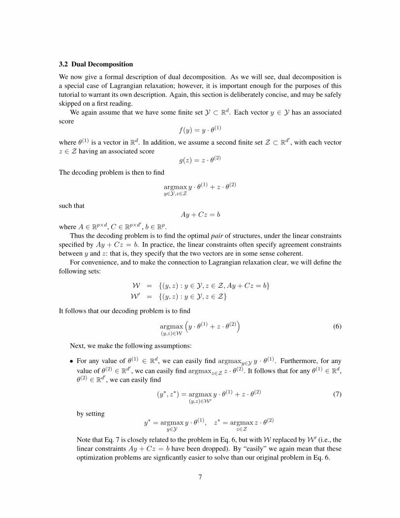
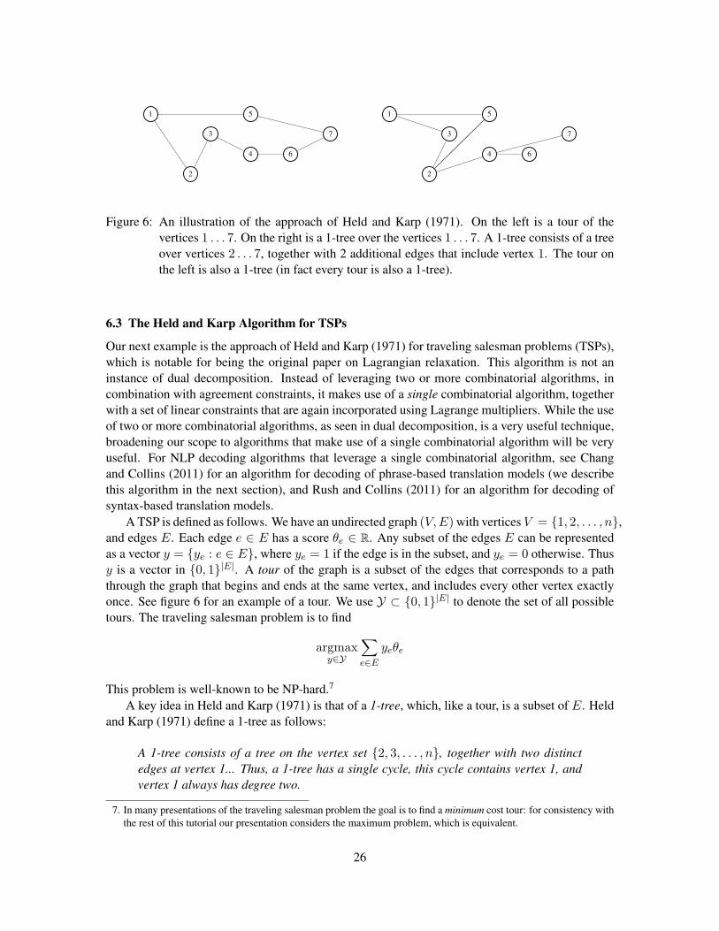
Figure 6: An illustration of the approach of Held and Karp (1971). On the left is a tour of thevertices 1 . . . 7. On the right is a 1-tree over the vertices 1 . . . 7. A 1-tree consists of a treeover vertices 2 . . . 7, together with 2 additional edges that include vertex 1. The tour onthe left is also a 1-tree (in fact every tour is also a 1-tree).

6.3 The Held and Karp Algorithm for TSPs

Our next example is the approach of Held and Karp (1971) for traveling salesman problems (TSPs),which is notable for being the original paper on Lagrangian relaxation. This algorithm is not aninstance of dual decomposition. Instead of leveraging two or more combinatorial algorithms, incombination with agreement constraints, it makes use of a single combinatorial algorithm, togetherwith a set of linear constraints that are again incorporated using Lagrange multipliers. While the useof two or more combinatorial algorithms, as seen in dual decomposition, is a very useful technique,broadening our scope to algorithms that make use of a single combinatorial algorithm will be veryuseful. For NLP decoding algorithms that leverage a single combinatorial algorithm, see Changand Collins (2011) for an algorithm for decoding of phrase-based translation models (we describethis algorithm in the next section), and Rush and Collins (2011) for an algorithm for decoding ofsyntax-based translation models.

A TSP is defined as follows. We have an undirected graph (V,E) with vertices V = {1, 2, . . . , n},and edges E. Each edge e 2 E has a score ✓e 2 R. Any subset of the edges E can be representedas a vector y = {ye : e 2 E}, where ye = 1 if the edge is in the subset, and ye = 0 otherwise. Thusy is a vector in {0, 1}|E|. A tour of the graph is a subset of the edges that corresponds to a paththrough the graph that begins and ends at the same vertex, and includes every other vertex exactlyonce. See figure 6 for an example of a tour. We use Y ⇢ {0, 1}|E| to denote the set of all possibletours. The traveling salesman problem is to find

argmaxy2Y

X

e2E

ye✓e

This problem is well-known to be NP-hard.7

A key idea in Held and Karp (1971) is that of a 1-tree, which, like a tour, is a subset of E. Heldand Karp (1971) define a 1-tree as follows:

A 1-tree consists of a tree on the vertex set {2, 3, . . . , n}, together with two distinctedges at vertex 1... Thus, a 1-tree has a single cycle, this cycle contains vertex 1, andvertex 1 always has degree two.

7. In many presentations of the traveling salesman problem the goal is to find a minimum cost tour: for consistency withthe rest of this tutorial our presentation considers the maximum problem, which is equivalent.

26

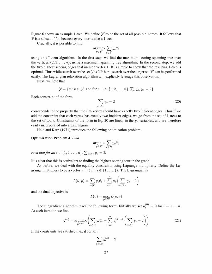
Figure 6 shows an example 1-tree. We define Y 0 to be the set of all possible 1-trees. It follows thatY is a subset of Y 0, because every tour is also a 1-tree.

Crucially, it is possible to findargmax

y2Y 0

X

e2E

ye✓e

using an efficient algorithm. In the first step, we find the maximum scoring spanning tree overthe vertices {2, 3, . . . , n}, using a maximum spanning tree algorithm. In the second step, we addthe two highest scoring edges that include vertex 1. It is simple to show that the resulting 1-tree isoptimal. Thus while search over the set Y is NP-hard, search over the larger set Y 0 can be performedeasily. The Lagrangian relaxation algorithm will explicitly leverage this observation.

Next, we note that

Y = {y : y 2 Y 0, and for all i 2 {1, 2, . . . , n},P

e:i2e ye = 2}

Each constraint of the form X

e:i2e

ye = 2 (20)

corresponds to the property that the i’th vertex should have exactly two incident edges. Thus if weadd the constraint that each vertex has exactly two incident edges, we go from the set of 1-trees tothe set of tours. Constraints of the form in Eq. 20 are linear in the ye variables, and are thereforeeasily incorporated into a Lagrangian.

Held and Karp (1971) introduce the following optimization problem:

Optimization Problem 4 Findargmax

y2Y 0

X

e2E

ye✓e

such that for all i 2 {1, 2, . . . , n},P

e:i2e ye = 2.

It is clear that this is equivalent to finding the highest scoring tour in the graph.As before, we deal with the equality constraints using Lagrange multipliers. Define the La-

grange multipliers to be a vector u = {ui : i 2 {1 . . . n}}. The Lagrangian is

L(u, y) =X

e2E

ye✓e +nX

i=1

ui

X

e:i2e

ye � 2

!

and the dual objective isL(u) = max

y2Y 0L(u, y)

The subgradient algorithm takes the following form. Initially we set u(0)i = 0 for i = 1 . . . n.

At each iteration we find

y(k) = argmaxy2Y 0

X

e2E

ye✓e +nX

i=1

u(k�1)i

X

e:i2e

ye � 2

!!

(21)

If the constraints are satisfied, i.e., if for all iX

e:i2e

y(k)e = 2

27

then the algorithm terminates, with a guarantee that the structure y(k) is the solution to optimizationproblem 4. Otherwise, a subgradient step is used to modify the Lagrange multipliers. It can beshown that the subgradient of L(u) at u is the vector g(u) defined as

g(u)(i) =X

e:i2e

y(u)e � 2

where y(u) = argmaxy2Y 0 L(u, y). Thus the subgradient step is for all i 2 {1 . . . n},

u(k)i = u

(k�1)i � �k

X

e:i2e

y(k)e � 2

!

(22)

Note that the problem in Eq. 21 is easily solved. It is equivalent to finding

y(k) = argmaxy2Y 0

X

e2E

ye✓0e

with modified edge weights ✓0e: for an edge e = {i, j}, we define

✓0e = ✓e + u(k�1)i + u

(k�1)j

Hence the new edge weights incorporate the Lagrange multipliers for the two vertices in the edge.The subgradient step in Eq. 22 has a clear intuition. For vertices with greater than 2 incident

edges in y(k), the value of the Lagrange multiplier ui is decreased, which will have the effect ofpenalising any edges including vertex i. Conversely, for vertices with fewer than 2 incident edges,ui will increase, and edges including that vertex will be preferred. The algorithm manipulates theui values in an effort to enforce the constraints that each vertex has exactly two incident edges.

We note that there is a qualitative difference between this example and our previous algorithms.Our previous algorithms had employed two sets of structures Y and Z , two optimization problems,and equality constraints enforcing agreement between the two structures. The TSP relaxation in-stead involves a single set Y . The two approaches are closely related, however, and similar theoremsapply to the TSP method (the proofs are trivial modifications of the previous proofs). We have

L(u) �X

e2E

y⇤e✓e

for all u, where y⇤ is the optimal tour. Under appropriate step sizes for the subgradient algorithm,we have

limk!1

L(u(k)) = minu

L(u)

Finally, if we ever find a structure y(k) that satisfies the linear constraints, then the algorithm hase-converged, and we have a guaranteed solution to the traveling salesman problem.

6.4 Phrase-based Translation

We next consider a Lagrangian relaxation algorithm, described by Chang and Collins (2011), fordecoding of phrase-based translation models (Koehn, Och, & Marcu, 2003). The input to a phrase-based translation model is a source-language sentence with n words, x = x1 . . . xn. The outputis a sentence in the target language. The examples in this section will use German as the sourcelanguage, and English as the target language. We will use the German sentence

28

wir m¨ussen auch diese kritik ernst nehmen

as a running example.A key component of a phrase-based translation model is a phrase-based lexicon, which pairs

sequences of words in the source language with sequences of words in the target language. Forexample, lexical entries that are relevent to the German sentence shown above include

(wir m¨ussen, we must)(wir m¨ussen auch, we must also)(ernst, seriously)

and so on. Each phrase entry has an associated score, which can take any value in the reals.We introduce the following notation. A phrase is a tuple (s, t, e), signifying that the subse-

quence xs . . . xt in the source language sentence can be translated as the target-language string e,using an entry from the phrase-based lexicon. For example, the phrase (1, 2, we must) would spec-ify that the sub-string x1 . . . x2 can be translated as we must. Each phrase p = (s, t, e) receives ascore ✓(p) 2 R under the model. For a given phrase p, we will use s(p), t(p) and e(p) to refer to itsthree components. We will use P to refer to the set of all possible phrases for the input sentence x.

A derivation y is then a finite sequence of phrases, p1, p2, . . . pL. The length L can be anypositive integer value. For any derivation y we use e(y) to refer to the underlying translation definedby y, which is derived by concatenating the strings e(p1), e(p2), . . . e(pL). For example, if

y = (1, 3, we must also), (7, 7, take), (4, 5, this criticism), (6, 6, seriously) (23)

then

e(y) = we must also take this criticism seriously

The score for any derivation y is then defined as

h(y) = g(e(y)) +X

p2y

✓(p)

where g(e(y)) is the score (log-probability) for e(y) under an n-gram language model.The set Y of valid derivations is defined as follows. For any derivation y, we define y(i) for

i = 1 . . . n to be the number of times that source word i is translated in the derivation. Moreformally,

y(i) =X

p2y

[[s(p) i t(p)]]

where [[⇡]] is 1 if the statement ⇡ is true, 0 otherwise. The set of valid derivations is then

Y = {y 2 P⇤ : for i = 1 . . . n, y(i) = 1}

where P⇤ is the set of finite length sequences of phrases. Thus for a derivation to be valid, eachsource-language word must be translated exactly once. Under this definition, the derivation in Eq. 23is valid. The decoding problem is then to find

y⇤ = argmaxy2Y

h(y) (24)

29

This problem is known to be NP-hard. Some useful intuition is as follows. A dynamic programmingapproach for this problem would need to keep track of a bit-string of length n specifying which ofthe n source language words have or haven’t been translated at each point in the dynamic program.There are 2n such bit-strings, resulting in the dynamic program having an exponential number ofstates.

We now describe the Lagrangian relaxation algorithm. As before, the key idea will be to definea set Y 0 such that Y is a subset of Y 0, and such that

argmaxy2Y 0

h(y) (25)

can be found efficiently. We do this by defining

Y 0 = {y 2 P⇤ :Pn

i=1 y(i) = n}

Thus derivations in Y 0 satisfy the weaker constraint that the total number of source words translatedis exactly n: we have dropped the y(i) = 1 constraints. As one example, the following derivationis a member of Y 0, but is not a member of Y:

y = (1, 3, we must also), (1, 2, we must), (3, 3, also), (6, 6, seriously) (26)

In this case we have y(1) = y(2) = y(3) = 2, y(4) = y(5) = y(7) = 0, and y(6) = 1. Hencesome words are translated more than once, and some words are translated 0 times.

Under this definition of Y 0, the problem in Eq. 25 can be solved efficiently, using dynamicprogramming. In contrast to the dynamic program for Eq. 24, which keeps track of a bit-string oflength n, the new dynamic program merely needs to keep track of how many source language wordshave been translated at each point in the search.

We proceed as follows. Note that

Y = {y : y 2 Y 0, and for i = 1 . . . n, y(i) = 1}

We introduce a Lagrange multiplier u(i) for each constraint y(i) = 1. The Lagrangian is

L(u, y) = h(y) +nX

i=1

u(i) (y(i)� 1)

The subgradient algorithm is as follows. Initially we set u(0)(i) = 0 for all i. At each iteration wefind

y(k) = argmaxy2Y 0

L(u(k�1), y) (27)

and perform the subgradient step

u(k)(i) = u(k�1)(i)� �k(y(k)(i)� 1) (28)

If at any point we have y(k)(i) = 1 for i = 1 . . . n, then we are guaranteed to have the optimalsolution to the original decoding problem.

30

The problem in Eq. 27 can be solved efficiently, because

argmaxy2Y 0

L(u(k�1), y)

= argmaxy2Y 0

0

@g(e(y)) +X

p2y

✓(p) +nX

i=1

u(k�1)(i) (y(i)� 1)

1

A

= argmaxy2Y 0

0

@g(e(y)) +X

p2y

✓0(p)

1

A

where

✓0(p) = ✓(p) +e(p)X

i=s(p)

u(k�1)(i)

Thus we have new phrase scores, ✓0(p), which take into account the Lagrange multiplier valuesfor positions s(p) . . . e(p). The subgradient step in Eq. 28 has a clear intuition. For any sourcelanguage word i that is translated more than once, the associated Lagrange multiplier u(i) willdecrease, causing phrases including word i to be penalised at the next iteration. Conversely, anyword translated 0 times will have its Lagrange multiplier increase, causing phrases including thatword to be preferred at the next iteration. The subgradient method manipulates the u(i) values inan attempt to force each source-language word to be translated exactly once.

The description we have given here is a sketch: Chang and Collins (2011) describe details of themethod, including a slightly more involved dynamic program that gives a tighter relaxation than themethod we have described here, and a tightening method that incrementally adds constraints whenthe method does not initially e-converge. The method is successful in recovering exact solutionsunder a phrase-based translation model, and is far more efficient than alternative approaches basedon general-purpose integer linear programming solvers.

7. Practical Issues

This section reviews various practical issues that arise with dual decomposition algorithms. Wedescribe diagnostics that can be used to track progress of the algorithm in minimizing the dual, andin providing a primal solution; we describe methods for choosing the step sizes, �k, in the algorithm;and we describe heuristics that can be used in cases where the algorithm does not provide an exactsolution. We will continue to use the algorithm from section 4 as a running example, although ourobservations are easily generalized to other Lagrangian relaxation algorithms.

The first thing to note is that each iteration of the algorithm produces a number of useful terms,in particular:

• The solutions y(k) and z(k).

• The current dual value L(u(k)) (which is equal to L(u(k), y(k), z(k)).

In addition, in cases where we have a function l : Y ! Z that maps each structure y 2 Y to astructure l(y) 2 Z , we also have

• A primal solution y(k), l(y(k)).

31

-19

-18

-17

-16

-15

-14

-13

0 10 20 30 40 50 60

Valu

e

Round

Current PrimalCurrent Dual

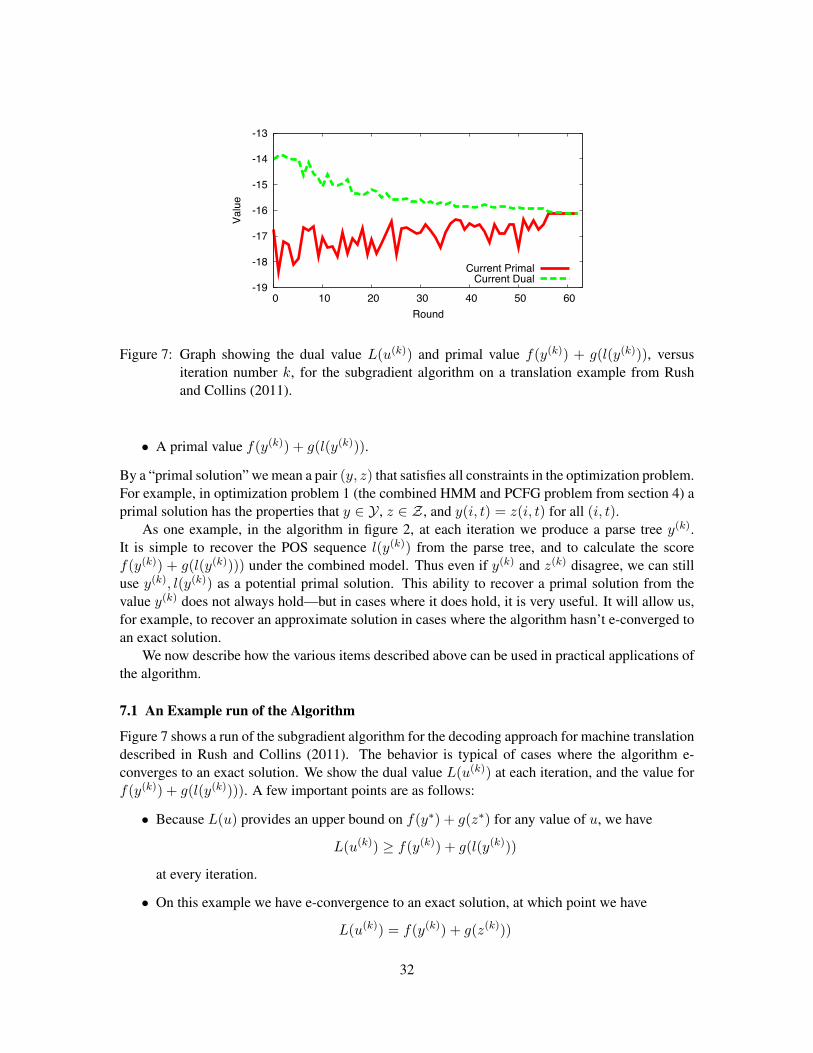
Figure 7: Graph showing the dual value L(u(k)) and primal value f(y(k)) + g(l(y(k))), versusiteration number k, for the subgradient algorithm on a translation example from Rushand Collins (2011).

• A primal value f(y(k)) + g(l(y(k))).

By a “primal solution” we mean a pair (y, z) that satisfies all constraints in the optimization problem.For example, in optimization problem 1 (the combined HMM and PCFG problem from section 4) aprimal solution has the properties that y 2 Y , z 2 Z , and y(i, t) = z(i, t) for all (i, t).

As one example, in the algorithm in figure 2, at each iteration we produce a parse tree y(k).It is simple to recover the POS sequence l(y(k)) from the parse tree, and to calculate the scoref(y(k)) + g(l(y(k)))) under the combined model. Thus even if y(k) and z(k) disagree, we can stilluse y(k), l(y(k)) as a potential primal solution. This ability to recover a primal solution from thevalue y(k) does not always hold—but in cases where it does hold, it is very useful. It will allow us,for example, to recover an approximate solution in cases where the algorithm hasn’t e-converged toan exact solution.

We now describe how the various items described above can be used in practical applications ofthe algorithm.

7.1 An Example run of the Algorithm

Figure 7 shows a run of the subgradient algorithm for the decoding approach for machine translationdescribed in Rush and Collins (2011). The behavior is typical of cases where the algorithm e-converges to an exact solution. We show the dual value L(u(k)) at each iteration, and the value forf(y(k)) + g(l(y(k)))). A few important points are as follows:

• Because L(u) provides an upper bound on f(y⇤) + g(z⇤) for any value of u, we have

L(u(k)) � f(y(k)) + g(l(y(k)))

at every iteration.

• On this example we have e-convergence to an exact solution, at which point we have

L(u(k)) = f(y(k)) + g(z(k)))

32

-19

-18

-17

-16

-15

-14

-13

0 10 20 30 40 50 60

Valu

e

Round

Best PrimalBest Dual

0

0.5

1

1.5

2

2.5

3

3.5

4

0 10 20 30 40 50 60

Valu

e

Round

Gap

Figure 8: The graph on the left shows the best dual value L⇤k and the best primal value p⇤k, versusiteration number k, for the subgradient algorithm on a translation example from Rush andCollins (2011). The graph on the right shows L⇤k � p⇤k plotted against k.

with (y(k), z(k)) guaranteed to be optimal (and in addition, with z(k) = l(y(k))).

• The dual values L(u(k)) are not monotonically decreasing—that is, for some iterations wehave

L(u(k+1)) > L(u(k))

even though our goal is to minimize L(u). This is typical: subgradient algorithms are not ingeneral guaranteed to give monotonically decreasing dual values. However, we do see thatfor most iterations the dual decreases—this is again typical.

• Similarly, the primal value f(y(k)) + g(z(k)) fluctuates (goes up and down) during the courseof the algorithm.

The following quantities can be useful in tracking progress of the algorithm at the k’th iteration:

• L(u(k)) � L(u(k�1)) is the change in the dual value from one iteration to the next. We willsoon see that this can be useful when choosing the step size for the algorithm (if this value ispositive, it may be an indication that the step size should decrease).

• L⇤k = mink0k L(u(k0)) is the best dual value found so far. It gives us the tightest upper boundon f(y⇤) + g(z⇤) that we have after k iterations of the algorithm.

• p⇤k = maxk0k f(y(k0)) + g(l(y(k0))) is the best primal value found so far.

• L⇤k�p⇤k is the gap between the best dual and best primal solution found so far by the algorithm.Because L⇤k � f(y⇤) + g(z⇤) � p⇤k, we have

L⇤k � p⇤k � f(y⇤) + g(z⇤)� p⇤k

hence the value for L⇤k�p⇤k gives us an upper bound on the difference between f(y⇤)+g(z⇤)and p⇤k. If L⇤k � p⇤k is small, we have a guarantee that we have a primal solution that is closeto being optimal.

Figure 8 shows a plot of L⇤k and p⇤k versus the number of iterations k for our previous exam-ple, and in addition shows a plot of the gap L⇤k � p⇤k. These graphs are, not surprisingly, muchsmoother than the graph in figure 7. In particular we are guaranteed that the values for L⇤k and p⇤kare monotonically decreasing and increasing respectively.

33

-16

-15.5

-15

-14.5

-14

-13.5

-13

0 5 10 15 20 25 30 35 40

Valu

e

Round

0.010.005

0.0005

Figure 9: Graph showing the dual value L(u(k)) versus the number of iterations k, for differentfixed step sizes.

7.2 Choice of the Step Sizes �k

Figure 9 shows convergence of the algorithm for various choices of step size, where we have chosento keep the stepsize constant at each iteration. We immediately see a potential dilemma arising.With too small a step size (� = 0.0005), convergence is smooth—the dual value is monotonicallydecreasing—but convergence is slow. With too large a step size (� = 0.01), convergence is muchfaster in the initial phases of the algorithm, but the dual then fluctuates quite erratically. In practiceit is often very difficult to choose a constant step size that gives good convergence properties in bothearly and late iterations of the algorithm.

Instead, we have found that we often find improved convergence properties with a choice ofstep size �k that decreases with increasing k. One possibility is to use a definition such as �k = c/kor �k = c/

pk where c > 0 is a constant. However these definitions can decrease the step size

too rapidly—in particular, they decrease the step size at all iterations, even in cases where progressis being made in decreasing the dual value. In many cases we have found that a more effectivedefinition is

�k =c

t + 1where c > 0 is again a constant, and t < k is the number of iterations prior to k where the dual valueincreases rather than decreases (i.e., the number of cases for k0 k where L(u(k0)) > L(u(k0�1))).Under this definition the step size decreases only when the dual value moves in the wrong direction.

7.3 Recovering Approximate Solutions

Figure 10 shows a run of the algorithm where we fail to get e-convergence to an exact solution. Insection 8.4 we will describe one possible strategy, namely tightening the relaxation, which can beused to produce an exact solution in these cases. Another obvious strategy, which is approximate,is to simply choose the best primal solution generated after k iterations of the algorithm, for somefixed k: i.e., to choose y(k0), l(y(k0)) where

k0 = argmaxk0k

f(y(k0)) + g(l(y(k0)))

34

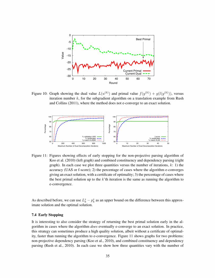
-30

-25

-20

-15

-10

-5

0

0 10 20 30 40 50 60 70

Valu

e

Round

Best Primal

Current PrimalCurrent Dual

Figure 10: Graph showing the dual value L(u(k)) and primal value f(y(k)) + g(l(y(k))), versusiteration number k, for the subgradient algorithm on a translation example from Rushand Collins (2011), where the method does not e-converge to an exact solution.

50

60

70

80

90

100

0 200 400 600 800 1000

Perc

enta

ge

Maximum Number of Dual Decomposition Iterations

% validation UAS% certificates

% match K=5000 50

60

70

80

90

100

0 10 20 30 40 50

Perc

enta

ge

Maximum Number of Dual Decomposition Iterations

f score% certificates

% match K=50

Figure 11: Figures showing effects of early stopping for the non-projective parsing algorithm ofKoo et al. (2010) (left graph) and combined constituency and dependency parsing (rightgraph). In each case we plot three quantities versus the number of iterations, k: 1) theaccuracy (UAS or f-score); 2) the percentage of cases where the algorithm e-convergesgiving an exact solution, with a certificate of optimality; 3) the percentage of cases wherethe best primal solution up to the k’th iteration is the same as running the algorithm toe-convergence.

As described before, we can use L⇤k � p⇤k as an upper bound on the difference between this approx-imate solution and the optimal solution.

7.4 Early Stopping

It is interesting to also consider the strategy of returning the best primal solution early in the al-gorithm in cases where the algorithm does eventually e-converge to an exact solution. In practice,this strategy can sometimes produce a high quality solution, albeit without a certificate of optimal-ity, faster than running the algorithm to e-convergence. Figure 11 shows graphs for two problems:non-projective dependency parsing (Koo et al., 2010), and combined constituency and dependencyparsing (Rush et al., 2010). In each case we show how three quantities vary with the number of

35

iterations of the algorithm. The first quantity is the percentage of cases where the algorithm e-converges, giving an exact solution, with a certificate of optimality. For combined constituency anddependency parsing it takes roughly 50 iterations for most (over 95%) of cases to e-converge; thesecond algorithm takes closer to 1000 iterations.

In addition, we show graphs indicating the quality of the best primal solution generated up toiteration k of the algorithm, versus the number of iterations, k. An “early stopping” strategy wouldbe to pick some fixed value for k, and to simply return the best primal solution generated in the first kiterations of the algorithm. We first plot the accuracy (f-score, or dependency accuracy respectively)for the two models under early stopping: we can see that accuracy very quickly asymptotes to itsoptimal value, suggesting that returning a primal solution before e-convergence can often yield highquality solutions. We also plot the percentage of cases where the primal solution returned is in factidentical to the primal solution returned when the algorithm is run to e-convergence. We again seethat this curve asymptotes quickly, showing that in many cases the early stopping strategy does infact produce the optimal solution, albeit without a certificate of optimality.

8. The Relationship to Linear Programming Relaxations

This section describes the close relationship between the dual decomposition algorithm and linearprogramming relaxations. This connection will be very useful in understanding the behavior of thealgorithm, and in particular in understanding the cases where the algorithm does not e-converge toan exact solution. In addition, it will suggest strategies for “tightening” the algorithm until an exactsolution is found.

8.1 The Linear Programming Relaxation

We continue to use the algorithm from section 4 as an example; the generalization to other problemsis straightforward. First, define the set

�y = {↵ : ↵ 2 R|Y|,X

y

↵y = 1,8y 0 ↵y 1}

Thus �y is a simplex, corresponding to the set of probability distributions over the finite set Y .Similarly, define

�z = {� : � 2 R|Z|,X

z

�z = 1,8z 0 �z 1}

as the set of distributions over the set Z .We now define a new optimization problem, as follows:

Optimization Problem 5 Find

max↵2�y ,�2�z

X

y

↵yf(y) +X

z

�zg(z) (29)

such that for all i, t, X

y

↵yy(i, t) =X

z

�zz(i, t) (30)

36

This optimization problem is a linear program: the objective in Eq. 29 is linear in the variables↵ and �; the constraints in Eq. 30, together with the constraints in the definitions of �y and �z , arealso linear in these variables.

This optimization problem is very similar to our original problem, optimization problem 1. Tosee this, define �0

y as follows:

�0y = {↵ : ↵ 2 R|Y|,

X

y

↵y = 1,8y ↵y 2 {0, 1}}

Thus �0y is a subset of �y, where the constraints 0 ↵y 1 have been replaced by ↵y 2 {0, 1}.

Define �0z similarly. Consider the following optimization problem, where we replace �y and �z in

Eq. 29 by �0y and �0

z respectively:

Optimization Problem 6 Find

max↵2�0

y ,�2�0z

X

y

↵yf(y) +X

z

�zg(z) (31)

such that for all i, t,X

y

↵yy(i, t) =X

z

�zz(i, t) (32)

This new problem is equivalent to our original problem, optimization problem 1: choosingvectors ↵ 2 �0

y and � 2 �0z is equivalent to choosing a single parse in Y , and a single POS

sequence in z. In this sense, optimization problem 5 is a relaxation of our original problem, whereconstraints of the form ↵y 2 {0, 1} and �z 2 {0, 1} are replaced with constraints of the form0 ↵y 1 and 0 �z 1.

Note that optimization problem 6 is an integer linear program, because the objective is againlinear in the ↵ and � variables, and the constraints on these variables combine linear constraintswith integer constraints (that each ↵y and �z must be either 0 or 1). It is also worth noting that �y

is actually the convex hull of the finite set �0y. The points in �0

y form the vertices of the polytope�y.

A useful theorem, which is central to the relationship between linear programming and combi-natorial optimization problems, is the following:

Theorem 6 For any finite set Y , and any function f : Y ! R,

maxy2Y

f(y) = max↵2�y

X

y2Y↵yf(y)

where �y is as defined above.

The proof is simple, and is given in appendix A.4.

37

8.2 The Dual of the New Optimization Problem

We now describe the dual problem for the linear program in Eqs. 29 and 30. This will again be afunction M(u) of a vector of dual variables u = {u(i, t) : i 2 {1 . . . n}, t 2 T }. A crucial resultwill be that the two dual functions M(u) and L(u) are identical.

Our new Lagrangian is

M(u, ↵,�) =X

y

↵yf(y) +X

z

�zg(z) +X

i,t

u(i, t)

X

y

↵yy(i, t)�X

z

�zz(i, t)

!

=

0

@X

y

↵yf(y) +X

i,t

u(i, t)X

y

↵yy(i, t)

1

A

+

0

@X

z

�zg(z)�X

i,t

u(i, t)X

z

�zz(i, t)

1

A

The new dual objective isM(u) = max

↵2�y ,�2�z

M(u, ↵,�)

Note that once again we have simply maximized out over the primal (↵ and �) variables, ignoringthe constraints in Eq. 30. The dual problem is to find

minu

M(u)

Two theorems regarding the dual problem are then as follows:

Theorem 7 Define (↵⇤, �⇤) to be the solution to the optimization problem in Eqs. 29 and 30. Then

minu

M(u) =X

y

↵⇤yf(y) +X

z

�⇤zg(z)

Proof. This follows immediately by results from linear programming duality, e.g., see Korte andVygen (2008).

Note that we now have equality in the above, in contrast to our previous result,

minu

L(u) � f(y⇤) + g(z⇤)

where the dual function only gave an upper bound on the best primal solution.Our second theorem is as follows:

Theorem 8 For any value of u,M(u) = L(u)

38

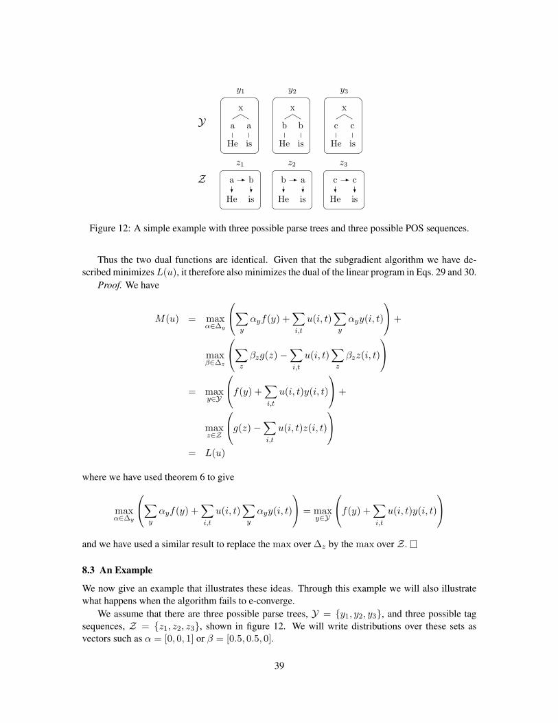
Yx

a

He

a

is

y1

x

b

He

b

is

y2

x

c

He

c

is

y3

Z a

He

b

is

z1

b

He

a

is

z2

c

He

c

is

z3

Figure 12: A simple example with three possible parse trees and three possible POS sequences.

Thus the two dual functions are identical. Given that the subgradient algorithm we have de-scribed minimizes L(u), it therefore also minimizes the dual of the linear program in Eqs. 29 and 30.

Proof. We have

M(u) = max↵2�y

0

@X

y

↵yf(y) +X

i,t

u(i, t)X

y

↵yy(i, t)

1

A+

max�2�z

0

@X

z

�zg(z)�X

i,t

u(i, t)X

z

�zz(i, t)

1

A

= maxy2Y

0

@f(y) +X

i,t

u(i, t)y(i, t)

1

A+

maxz2Z

0

@g(z)�X

i,t

u(i, t)z(i, t)

1

A

= L(u)

where we have used theorem 6 to give

max↵2�y

0

@X

y

↵yf(y) +X

i,t

u(i, t)X

y

↵yy(i, t)

1

A = maxy2Y

0

@f(y) +X

i,t

u(i, t)y(i, t)

1

A

and we have used a similar result to replace the max over �z by the max over Z .

8.3 An Example

We now give an example that illustrates these ideas. Through this example we will also illustratewhat happens when the algorithm fails to e-converge.

We assume that there are three possible parse trees, Y = {y1, y2, y3}, and three possible tagsequences, Z = {z1, z2, z3}, shown in figure 12. We will write distributions over these sets asvectors such as ↵ = [0, 0, 1] or � = [0.5, 0.5, 0].

39

Yx

a

He

a

is

y1

x

b

He

b

is

y2

x

c

He

c

is

y3

Z a

He

b

is

z1

b

He

a

is

z2

c

He

c

is

z3

Yx

a

He

a

is

y1

x

b

He

b

is

y2

x

c

He

c

is

y3

Z a

He

b

is

z1

b

He

a

is

z2

c

He

c

is

z3

Figure 13: Illustration of two solutions that satisfy the constraints in Eq. 30. On the left, the solution↵ = [0, 0, 1], � = [0, 0, 1] puts weight 1 on y3 and z3. On the right, the fractionalsolution ↵ = [0.5, 0.5, 0] and � = [0.5, 0.5, 0] puts 0.5 weight on y1/y2 and z1/z2.

Now consider pairs of vectors (↵,�) that satisfy the constraints in Eq. 30. Figure 13 illustratestwo possible solutions. One such pair, which we will denote as (↵1, �1), is ↵1 = [0, 0, 1], �1 =[0, 0, 1]. It is easily verified that under this definition

X

y2Y↵1

yy(1, c) =X

z2Y�1

zz(1, c) =X

y2Y↵1

yy(2, c) =X

z2Y�1

zz(2, c) = 1

with all other expected values being equal to 0: hence (↵1, �1) satisfies the constraints. This po-tential solution is integral, in that it puts weight 1 on a single parse tree/pos-tag sequence, with allother structures having weight 0.

A second pair that satisfies the constraints is ↵2 = [0.5, 0.5, 0], �2 = [0.5, 0.5, 0]. Under thesedefinitions,

X

y2Y↵2

yy(1, a) =X

z2Y�2

zz(1, a) =X

y2Y↵2

yy(1, b) =X

z2Y�2

zz(1, b) = 0.5

and X

y2Y↵2

yy(2, a) =X

z2Y�2

zz(2, a) =X

y2Y↵2

yy(2, b) =X

z2Y�2

zz(2, b) = 0.5

with all other expected values being equal to 0. The pair (↵2, �2) is a fractional solution, in that itputs fractional (0.5) weight on some structures.

Next, consider different definitions for the functions f(y) and g(z). Consider first the definitionsf = [0, 0, 1] and g = [0, 0, 1] (we write f = [0, 0, 1] as shorthand for f(y1) = 0, f(y2) = 0,f(y3) = 1). The solution to the problem in Eqs. 29 and 30 is then the pair (↵1, �1).

Alternatively, consider the definitions f = [1, 1, 2] and g = [1, 1,�2]. In this case the followingsituation arises:

• The pair (↵1, �1) achieves score 0 under the objective in Eq. 29, whereas the pair (↵2, �2)achieves a score of 2. Thus the solution to the problem in Eqs. 29 and 30 is (↵2, �2), which isa fractional solution.

• By theorem 7, minu M(u) is equal to the value for the optimal primal solution, i.e., minu M(u) =2. Hence minu L(u) = 2.

40

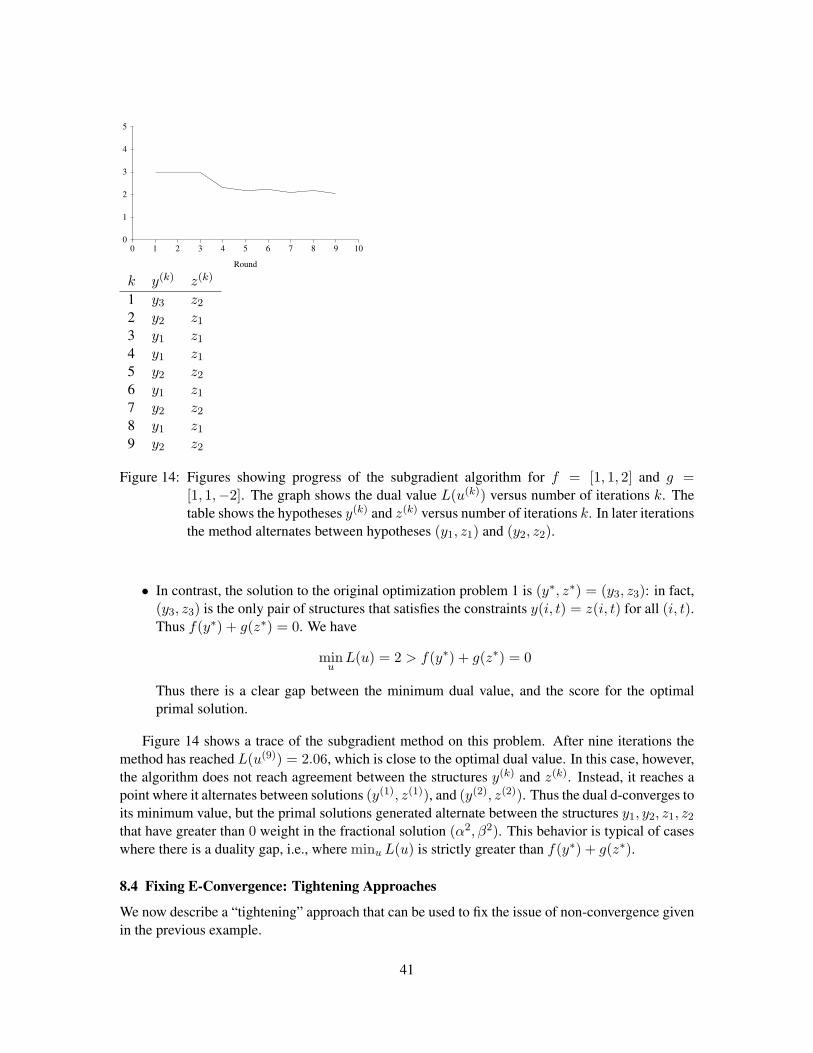
0 1 2 3 4 5 6 7 8 9 100

1

2

3

4

5

Round

k y(k) z(k)

1 y3 z2

2 y2 z1

3 y1 z1

4 y1 z1

5 y2 z2

6 y1 z1

7 y2 z2

8 y1 z1

9 y2 z2

Figure 14: Figures showing progress of the subgradient algorithm for f = [1, 1, 2] and g =[1, 1,�2]. The graph shows the dual value L(u(k)) versus number of iterations k. Thetable shows the hypotheses y(k) and z(k) versus number of iterations k. In later iterationsthe method alternates between hypotheses (y1, z1) and (y2, z2).

• In contrast, the solution to the original optimization problem 1 is (y⇤, z⇤) = (y3, z3): in fact,(y3, z3) is the only pair of structures that satisfies the constraints y(i, t) = z(i, t) for all (i, t).Thus f(y⇤) + g(z⇤) = 0. We have

minu

L(u) = 2 > f(y⇤) + g(z⇤) = 0

Thus there is a clear gap between the minimum dual value, and the score for the optimalprimal solution.

Figure 14 shows a trace of the subgradient method on this problem. After nine iterations themethod has reached L(u(9)) = 2.06, which is close to the optimal dual value. In this case, however,the algorithm does not reach agreement between the structures y(k) and z(k). Instead, it reaches apoint where it alternates between solutions (y(1), z(1)), and (y(2), z(2)). Thus the dual d-converges toits minimum value, but the primal solutions generated alternate between the structures y1, y2, z1, z2

that have greater than 0 weight in the fractional solution (↵2, �2). This behavior is typical of caseswhere there is a duality gap, i.e., where minu L(u) is strictly greater than f(y⇤) + g(z⇤).

8.4 Fixing E-Convergence: Tightening Approaches

We now describe a “tightening” approach that can be used to fix the issue of non-convergence givenin the previous example.

41

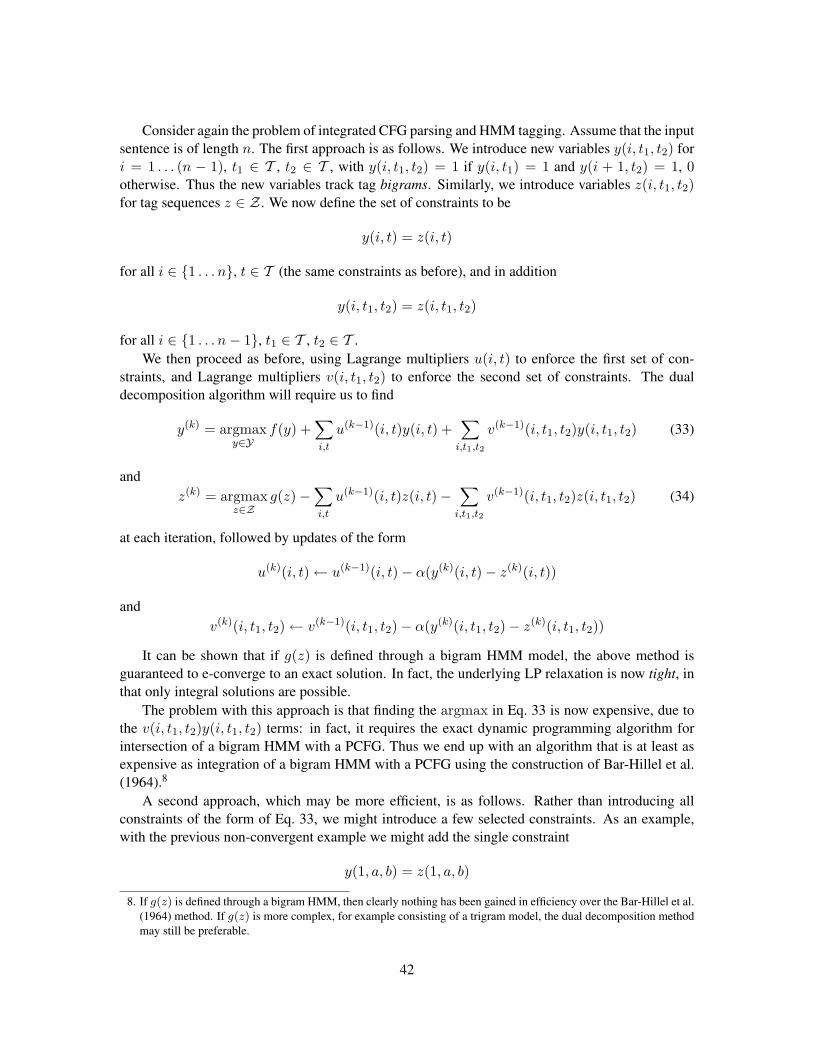
Consider again the problem of integrated CFG parsing and HMM tagging. Assume that the inputsentence is of length n. The first approach is as follows. We introduce new variables y(i, t1, t2) fori = 1 . . . (n � 1), t1 2 T , t2 2 T , with y(i, t1, t2) = 1 if y(i, t1) = 1 and y(i + 1, t2) = 1, 0otherwise. Thus the new variables track tag bigrams. Similarly, we introduce variables z(i, t1, t2)for tag sequences z 2 Z . We now define the set of constraints to be

y(i, t) = z(i, t)

for all i 2 {1 . . . n}, t 2 T (the same constraints as before), and in addition

y(i, t1, t2) = z(i, t1, t2)

for all i 2 {1 . . . n� 1}, t1 2 T , t2 2 T .We then proceed as before, using Lagrange multipliers u(i, t) to enforce the first set of con-

straints, and Lagrange multipliers v(i, t1, t2) to enforce the second set of constraints. The dualdecomposition algorithm will require us to find

y(k) = argmaxy2Y

f(y) +X

i,t

u(k�1)(i, t)y(i, t) +X

i,t1,t2

v(k�1)(i, t1, t2)y(i, t1, t2) (33)

andz(k) = argmax

z2Zg(z)�

X

i,t

u(k�1)(i, t)z(i, t)�X

i,t1,t2

v(k�1)(i, t1, t2)z(i, t1, t2) (34)

at each iteration, followed by updates of the form

u(k)(i, t) u(k�1)(i, t)� ↵(y(k)(i, t)� z(k)(i, t))

andv(k)(i, t1, t2) v(k�1)(i, t1, t2)� ↵(y(k)(i, t1, t2)� z(k)(i, t1, t2))

It can be shown that if g(z) is defined through a bigram HMM model, the above method isguaranteed to e-converge to an exact solution. In fact, the underlying LP relaxation is now tight, inthat only integral solutions are possible.

The problem with this approach is that finding the argmax in Eq. 33 is now expensive, due tothe v(i, t1, t2)y(i, t1, t2) terms: in fact, it requires the exact dynamic programming algorithm forintersection of a bigram HMM with a PCFG. Thus we end up with an algorithm that is at least asexpensive as integration of a bigram HMM with a PCFG using the construction of Bar-Hillel et al.(1964).8

A second approach, which may be more efficient, is as follows. Rather than introducing allconstraints of the form of Eq. 33, we might introduce a few selected constraints. As an example,with the previous non-convergent example we might add the single constraint

y(1, a, b) = z(1, a, b)

8. If g(z) is defined through a bigram HMM, then clearly nothing has been gained in efficiency over the Bar-Hillel et al.(1964) method. If g(z) is more complex, for example consisting of a trigram model, the dual decomposition methodmay still be preferable.

42

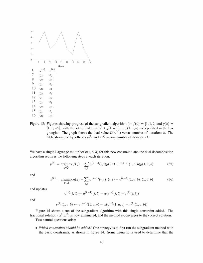
7 8 9 10 11 12 13 14 15 160

1

2

3

4

5

Round

k y(k) z(k)

7 y3 z2

8 y2 z3

9 y1 z2

10 y3 z1

11 y2 z3

12 y1 z2

13 y3 z1

14 y2 z3

15 y1 z2

16 y3 z3

Figure 15: Figures showing progress of the subgradient algorithm for f(y) = [1, 1, 2] and g(z) =[1, 1,�2], with the additional constraint y(1, a, b) = z(1, a, b) incorporated in the La-grangian. The graph shows the dual value L(u(k)) versus number of iterations k. Thetable shows the hypotheses y(k) and z(k) versus number of iterations k.

We have a single Lagrange multiplier v(1, a, b) for this new constraint, and the dual decompositionalgorithm requires the following steps at each iteration:

y(k) = argmaxy2Y

f(y) +X

i,t

u(k�1)(i, t)y(i, t) + v(k�1)(1, a, b)y(1, a, b) (35)

andz(k) = argmax

z2Zg(z)�

X

i,t

u(k�1)(i, t)z(i, t)� v(k�1)(1, a, b)z(1, a, b) (36)

and updatesu(k)(i, t) u(k�1)(i, t)� ↵(y(k)(i, t)� z(k)(i, t))

andv(k)(1, a, b) v(k�1)(1, a, b)� ↵(y(k)(1, a, b)� z(k)(1, a, b))

Figure 15 shows a run of the subgradient algorithm with this single constraint added. Thefractional solution (↵2, �2) is now eliminated, and the method e-converges to the correct solution.

Two natural questions arise:

• Which constraints should be added? One strategy is to first run the subgradient method withthe basic constraints, as shown in figure 14. Some heuristic is used to determine that the

43

dual is no longer decreasing at a significant rate. At that point, it can be determined thatthe algorithm is oscillating between solutions (y1, z1) and (y2, z2), and that the additionalconstraint y(1, a, b) = z(1, a, b) would rule out these solutions; hence this constraint is added.

• When is this more efficient than adding all constraints in Eq. 33? Our toy example is toosimple to illustrate the benefit of only adding selected constraints. To understand the benefit,consider the case where the sentence length n is reasonably large. In that case, we mightadd bigram constraints at only a few positions in the sentence: in practice the CKY decodingalgorithm will only need to introduce the Bar-Hillel et al. (1964) machinery at these selectedpoints, which can be much more efficient that introducing all constraints.

For examples of methods that tighten dual decomposition/Lagrangian relaxation techniques us-ing additional constraints, see Rush and Collins (2011), Chang and Collins (2011).

8.5 Compact Linear Programs

The LP relaxations that we have described have a very large set of variables: that is, one variablefor each member of Y and Z . In most cases of interest, the sets Y and Z will be exponential in size.

In this section we describe how to derive equivalent linear programs with far fewer variables.This is a problem of practical interest: for many problems, we have found it beneficial to implementthe underlying LP relaxation within a generic LP solver, as a way of debugging dual decompositionalgorithms. This is practical with the compact LPs that we describe in this section, but is clearlyimpractical with the exponential-size linear programs described in the previous section.

First, consider the abstract description of Lagrangian relaxation given in section 3. The LPrelaxation was

argmaxµ2Q

µ · ✓

whereQ = {y : y 2 Conv(Y 0) and Ay = b}

where A 2 Rp⇥d and b 2 Rp. Recall that Conv(Y 0) is the convex hull of the set Y 0. Next, assumethat Conv(Y 0) can itself be defined through a polynomial number of linear constraints: that is,

Conv(Y 0) = {y 2 Rd : Cy = e, y � 0} (37)

for some C 2 Rq⇥d and e 2 Rq, where the number of constraints, q, is polynomial. In this case wehave an explicit characterization of the set Q as

Q = {y 2 Rd : Cy = e, y � 0 and Ay = b}

Because d, p, and q are all polynomial in size, the resulting linear program is polynomial in size. Inthis sense it is “compact”.

The remaining question is whether a characterization of the form of Eq. 37 exists, and if so, howit is defined. Recall that we made the assumption that for any value of ✓,

argmaxy2Y 0

y · ✓ (38)

44

can be found using a combinatorial algorithm. For many combinatorial algorithms, there are LPformulations that are polynomial in size: these formulations lead directly to definitions of C and e.9

For example, Martin, Rardin, and Campbell (1990) give such a construction for dynamic program-ming algorithms, which includes weighted context-free grammars, the Viterbi algorithm, and otherdynamic programs used in NLP. Magnanti and Wolsey (1994) describe a construction for directedspanning trees, as used by Martins, Smith., and Xing (2009) within the context of non-projectivedependency parsing. Korte and Vygen (2008) describe many other such constructions. In short,given a combinatorial algorithm that solves the problem in Eq. 38, it is often straightforward to finda recipe for constructing a pair (C, e) that completely characterizes Conv(Y 0).

It is straightforward to extend this idea to the LP for dual decomposition. Consider again ourrunning example, (optimization problem 1),

argmaxy2Y,z2Z

f(y) + g(z)

such that for all i = 1 . . . n, t 2 T ,y(i, t) = z(i, t)

Rush et al. (2010) give a full description of the compact LP for this problem: we give a sketch here.Define each y to be a vector in {0, 1}d that specifies which context-free rules y contains. It

follows that Y is a subset of {0, 1}d. We then have

f(y) = y · ✓

where ✓ 2 Rd is a vector specifying the weight for each rule. Similarly, define z to be a vector in{0, 1}d0 that specifies the trigrams that z contains (assuming that g(z) is a trigram tagging model).It follows that Z is a subset of {0, 1}d0 . We can then write

g(z) = z · ✓0

for some ✓0 2 Rd0 . The compact LP is then

argmaxµ2Conv(Y),⌫2Conv(Z)

µ · ✓ + ⌫ · ✓0

such that for all i = 1 . . . n, t 2 T ,µ(i, t) = ⌫(i, t)

Again, the existence of combinatorial algorithms for the problems argmaxy2Y y·✓ and argmaxz2Z z·✓0 implies explicit representations

Conv(Y) = {µ 2 Rd : Aµ = b, µ � 0}

andConv(Z) = {⌫ 2 Rd0 : C⌫ = e, ⌫ � 0}

where A, b, C and e are polynomial in size. Rush et al. (2010) describe this construction in detailfor the case where a weighted CFG is combined with a finite-state tagger.

9. There is one subtlety here: in some cases additional auxilliary variables may need to be introduced. See for examplethe construction from Magnanti and Wolsey (1994) for directed spanning trees. However the number of auxilliaryvariables is generally polynomial in number, hence this is benign.

45

8.6 Summary

To summarize, the key points of this section were as follows:

• We introduced a linear programming problem that was a relaxation of our original problem.The function L(u) was shown to be the dual of this linear programming relaxation.

• In cases where the optimal solution to the underlying LP is fractional, the subgradient methodwill still d-converge to minu L(u). However the primal solutions (y(k), z(k)) will alternatebetween different solutions that do not satisfy the y(i, t) = z(i, t) constraints.

• In practice, tightening methods can be used to improve convergence. These methods selec-tively introduce constraints in an effort to improve convergence of the method, with the costof increased complexity in finding y(k) and/or z(k). The precise constraints to be added can bechosen by identifying constraints that are frequently violated during the subgradient method.

• Finally, we described methods that construct a compact linear program that is equivalent tothe original LP relaxation. This linear program is often small enough to be solved by a genericLP solver; this can be useful in debugging dual decomposition or Lagrangian relaxation algo-rithms.

9. Conclusions

A broad class of inference problems in statistical NLP and other areas of machine learning areamenable to Lagrangian relaxation (LR) methods. LR methods make use of combinatorial algo-rithms in combination with linear constraints that are introduced using Lagrange multipliers: it-erative methods are used to minimize the resulting dual objective. LR algorithms are simple andefficient, typically involving repeated applications of the underlying combinatorial algorithm, inconjunction with simple additive updates to the Lagrange multipliers. They have well-understoodformal properties: the dual objective is an upper bound on the score for the optimal primal solution;there are close connections to linear programming relaxations; and crucially, they have the potentialof producing an exact solution to the original inference problem, with a certificate of optimality. Ex-periments on several NLP problems have shown the effectiveness of LR algorithms for inference:LR methods are often considerably more efficient than existing exact methods, and have strongerformal guarantees than the approximate search methods that are often used in practice.

Appendix A. Proofs

In this section we derive various results for the combined parsing and tagging problem. Recall thatin this case the Lagrangian is defined as

L(u, y, z) = f(y) + g(z) +X

i2{1...n},t2Tu(i, t)(y(i, t)� z(i, t))

and that the dual objective is L(u) = maxy2Y,z2Z L(u, y, z). Here n is the number of words in thesentence, and T is a finite set of part-of-speech tags.

We first prove that L(u) is a convex function; we then derive the expression for subgradientsof L(u); we then give a convergence theorem for the algorithm in figure 2, which is a subgradientalgorithm for minimization of L(u).

46

Finally, we give a proof of theorem 6.

A.1 Proof of Convexity of L(u)

The theorem is as follows:

Theorem 9 L(u) is convex. That is, for any u(1) 2 Rd, u(2) 2 Rd, � 2 [0, 1],

L(�u(1) + (1� �)u(2)) �L(u(1)) + (1� �)L(u(2))

Proof: Define(y⇤, z⇤) = arg max

y2Y,z2ZL(u⇤, y, z)

where u⇤ = �u(1) + (1� �)u(2). It follows that

L(u⇤) = L(u⇤, y⇤, z⇤)

In addition, note that

L(u(1), y⇤, z⇤) maxy2Y,z2Z

L(u(1), y, z) = L(u(1))

and similarlyL(u(2), y⇤, z⇤) L(u(2))

from which it follows that

�L(u(1), y⇤, z⇤) + (1� �)L(u(2), y⇤, z⇤) �L(u(1)) + (1� �)L(u(2))

Finally, it is easy to show that

�L(u(1), y⇤, z⇤) + (1� �)L(u(2), y⇤, z⇤) = L(u⇤, y⇤, z⇤) = L(u⇤)

henceL(u⇤) �L(u(1)) + (1� �)L(u(2))

which is the desired result.

A.2 Subgradients of L(u)

For any value of u 2 Rd, as before define

(y(u), z(u)) = argmaxy2Y,z2Z

L(u, y, z)

or equivalently,

y(u) = argmaxy2Y

0

@f(y) +X

i,t

u(i, t)y(i, t)

1

A

and

z(u) = argmaxz2Z

0

@g(z)�X

i,t

u(i, t)z(i, t)

1

A

47

Then if we define �(u) as the vector with components

�(u)(i, t) = y(u)(i, t)� z(u)(i, t)

for i 2 {1 . . . n}, t 2 T , then �(u) is a subgradient of L(u) at u.This result is a special case of the following theorem:10

Theorem 10 Define the function L : Rd ! R as

L(u) = maxi2{1...m}

(ai · u + bi)

where ai 2 Rd and bi 2 R for i 2 {1 . . . m}. Then for any value of u, if

j = argmaxi2{1...m}

(ai · u + bi)

then aj is a subgradient of L(u) at u.

Proof: For aj to be a subgradient at the point u, we need to show that for all v 2 Rd,

L(v) � L(u) + aj · (v � u)

Equivalently, we need to show that for all v 2 Rd,

maxi2{1...m}

(ai · v + bi) � maxi2{1...m}

(ai · u + bi) + aj · (v � u) (39)

To show this, first note that

aj · u + bj = maxi2{1...m}

(ai · u + bi)

hencemax

i2{1...m}(ai · u + bi) + aj · (v � u) = bj + aj · v max

i2{1...m}(ai · v + bi)

thus proving the theorem.

A.3 Convergence Proof for the Subgradient Method

Consider a convex function L : Rd ! R, which has a minimizer u⇤ (i.e., u⇤ = argminu2Rd L(u)).

The subgradient method is an iterative method which initializes u to some value u(0) 2 Rd, thensets

u(k+1) = u(k) � �kgk

for k = 0, 1, 2, . . ., where �k > 0 is the stepsize at the k’th iteration, and gk is a subgradient at u(k):that is, for all v 2 Rd,

L(v) � L(u(k)) + gk · (v � u(k))

The following theorem will then be very useful in proving convergence of the method (thetheorem and proof is taken from Boyd and Mutapcic (2007)):

10. To be specific, our definition of L(u) can be written in the form maxi2{1...m} (ai · u + bi) as follows. Define theinteger m to be |Y|⇥ |Z|. Define (y(i), z(i)

) for i 2 {1 . . . m} to be a list of all possible pairs (y, z) such that y 2 Yand z 2 Z . Define bi = f(y(i)

) + g(z(i)), and ai to be the vector with components ai(l, t) = y(i)

(l, t)� z(i)(l, t)

for l 2 {1 . . . n}, t 2 T . Then it can be verifed that L(u) = maxi2{1...m} (ai · u + bi).

48

Theorem 11 Assume that for all k, ||gk||2 G2 where G is some constant. Then for any k � 0,

mini2{0...k}

L(u(i)) L(u⇤) +||u(0) � u⇤||2 + G2Pk

i=0 �2i

2Pk

i=0 �i

Proof: First, given the updates u(k+1) = u(k) � �kgk, we have for all k � 0,

||u(k+1) � u⇤||2 = ||u(k) � �kgk � u⇤||2

= ||u(k) � u⇤||2 � 2�kgk · (u(k) � u⇤) + �2k||gk||2

By the subgradient property,

L(u⇤) � L(u(k)) + gk · (u⇤ � u(k))

hence�gk · (u(k) � u⇤) L(u⇤)� L(u(k))

Using this inequality, together with ||gk||2 G2, gives

||u(k+1) � u⇤||2 ||u(k) � u⇤||2 + 2�k

⇣L(u⇤)� L(u(k))

⌘+ �2

kG2

Taking a sum over both sides of i = 0 . . . k giveskX

i=0

||u(i+1) � u⇤||2 kX

i=0

||u(i) � u⇤||2 + 2kX

i=0

�i

⇣L(u⇤)� L(u(i))

⌘+

kX

i=0

�2i G

2

and hence

||u(k+1) � u⇤||2 ||u(0) � u⇤||2 + 2kX

i=0

�i

⇣L(u⇤)� L(u(i))

⌘+

kX

i=0

�2i G

2

Finally, using ||u(k+1) � u⇤||2 � 0 andkX

i=0

�i

⇣L(u⇤)� L(u(i))

⌘

kX

i=0

�i

!

L(u⇤)� mini2{0...k}

L(u(i))

!

gives

0 ||u(0) � u⇤||2 + 2

kX

i=0

�i

!

L(u⇤)� mini2{0...k}

L(u(i))

!

+kX

i=0

�2i G

2

Rearranging terms gives the result in the theorem.This theorem has a number of consequences. As one example, for a constant step-size, �k = h

for some h > 0,

limk!1

||u(0) � u⇤||2 + G2Pk

i=1 �2i

2Pk

i=1 �i

!

=Gh

2

hence in the limit the value formin

i2{1...k}L(u(i))

is within Gh/2 of the optimal solution. A slightly more involved argument shows that under theassumptions that �k > 0, limk!1 �k = 0, and

P1k=0 �k =1,

limk!1

||u(0) � u⇤||2 + G2Pk

i=1 �2i

2Pk

i=1 �i

!

= 0

See Boyd and Mutapcic (2007) for the full derivation.

49

A.4 Proof of Theorem 6

Recall that our goal is to prove that

maxy2Y

f(y) = max↵2�y

X

y2Y↵yf(y)

We will show this by proving: (1) maxy2Y f(y) max↵2�y

Py2Y ↵yf(y), and (2) maxy2Y f(y) �

max↵2�y

Py2Y ↵yf(y).

First, consider case (1). Define y⇤ to be a member of Y such that

f(y⇤) = maxy2Y

f(y)

Next, define ↵y⇤ = 1, and ↵y = 0 for y 6= y⇤. Then we haveX

y2Y↵yf(y) = f(y⇤)

Hence we have found a setting for the ↵ variables such thatX

y2Y↵yf(y) = max

y2Yf(y)

from which it follows thatmax↵2�y

X

y2Y↵yf(y) � max

y2Yf(y)

Next, consider case (2). Define ↵⇤ to be a setting of the ↵ variables such thatX

y

↵⇤yf(y) = max↵2�y

X

y2Y↵yf(y)

Next, define y⇤ to be a member of Y such that

f(y⇤) = maxy:↵⇤

y>0f(y)

It is easily verified thatf(y⇤) �

X

y

↵⇤yf(y)

Hence we have found a y⇤ 2 Y such that

f(y⇤) � max↵2�y

X

y

↵⇤yf(y)

from which it follows thatmaxy2Y

f(y) � max↵2�y

X

y

↵⇤yf(y)

50

References

Auli, M., & Lopez, A. (2011). A comparison of loopy belief propagation and dual decompositionfor integrated ccg supertagging and parsing. In Proceedings of the 49th Annual Meeting ofthe Association for Computational Linguistics: Human Language Technologies, pp. 470–480,Portland, Oregon, USA. Association for Computational Linguistics.

Bar-Hillel, Y., Perles, M., & Shamir, E. (1964). On formal properties of simple phrase structuregrammars. In Language and Information: Selected Essays on their Theory and Application,pp. 116–150.

Boyd, S., & Mutapcic, A. (2007). Subgradient Methods. Course Notes for EE364b, StanfordUniversity, Winter 2006-07.

Chang, Y., & Collins, M. (2011). Exact Decoding of Phrase-based Translation Models throughLagrangian Relaxation. In To appear proc. of EMNLP.

Collins, M. (1997). Three Generative, Lexicalised Models for Statistical Parsing. In Proc. ACL, pp.16–23.

DeNero, J., & Macherey, K. (2011). Model-Based Aligner Combination Using Dual Decomposi-tion. In Proc. ACL.

Duchi, J., Tarlow, D., Elidan, G., & Koller, D. (2007). Using combinatorial optimization within max-product belief propagation. In Advances in Neural Information Processing Systems (NIPS).

Fisher, M. L. (1981). The lagrangian relaxation method for solving integer programming problems.Management Science, 27(1), pp. 1–18.

Held, M., & Karp, R. M. (1971). The traveling-salesman problem and minimum spanning trees:Part ii. Mathematical Programming, 1, 6–25. 10.1007/BF01584070.

Johnson, J., Malioutov, D., & Willsky, A. (2007). Lagrangian relaxation for map estimation ingraphical models. In 45th Annual Allerton Conference on Communication, Control and Com-puting.

Jojic, V., Gould, S., & Koller, D. (2010). Fast and smooth: Accelerated dual decomposition forMAP inference. In Proceedings of International Conference on Machine Learning (ICML).

Klein, D., & Manning, C. (2002). Fast exact inference with a factored model for natural languageparsing. Advances in neural information processing systems, 15(2002).

Koehn, P., Och, F. J., & Marcu, D. (2003). Statistical phrase-based translation. In Proceedings ofthe 2003 Conference of the North American Chapter of the Association for ComputationalLinguistic s on Human Language Technology, NAACL ’03, pp. 48–54.

Komodakis, N., Paragios, N., & Tziritas, G. (2007). MRF Optimization via Dual Decomposition:Message-Passing Revisited. In Proc. ICCV.

Komodakis, N., Paragios, N., & Tziritas, G. (2010). Mrf energy minimization and beyond via dualdecomposition. IEEE Transactions on Pattern Analysis and Machine Intelligence.

Koo, T., Carreras, X., & Collins, M. (2008). Simple semi-supervised dependency parsing. In Proc.ACL/HLT.

Koo, T., Rush, A. M., Collins, M., Jaakkola, T., & Sontag, D. (2010). Dual decomposition forparsing with non-projective head automata. In EMNLP.

51

Korte, B., & Vygen, J. (2008). Combinatorial Optimization: Theory and Algorithms. SpringerVerlag.

Lafferty, J., McCallum, A., & Pereira, F. (2001). Conditional Random Fields: Probabilistic Modelsfor Segmenting and Labeling Sequence Data. In Proc. ICML, pp. 282–289.

Lemarechal, C. (2001). Lagrangian Relaxation. In Computational Combinatorial Optimization, Op-timal or Provably Near-Optimal Solutions [based on a Spring School], pp. 112–156, London,UK. Springer-Verlag.

Magnanti, T. L., & Wolsey, L. A. (1994). Optimal trees. Tech. rep. 290-94, Massachusetts Instituteof Technology, Operations Research Center.

Martin, R., Rardin, R., & Campbell, B. (1990). Polyhedral characterization of discrete dynamicprogramming. Operations research, 38(1), 127–138.

Martins, A., Smith., N., & Xing, E. (2009). Concise Integer Linear Programming Formulations forDependency Parsing. In Proc. ACL, pp. 342–350.

Martins, A., Smith, N., Figueiredo, M., & Aguiar, P. (2011). Dual decomposition with many over-lapping components. In Proceedings of the 2011 Conference on Empirical Methods in NaturalLanguage Processing, pp. 238–249, Edinburgh, Scotland, UK. Association for ComputationalLinguistics.

McDonald, R. (2006). Discriminative Training and Spanning Tree Algorithms for DependencyParsing. Ph.D. thesis, University of Pennsylvania, Philadelphia, PA, USA.

Nedic, A., & Ozdaglar, A. (2009). Approximate primal solutions and rate analysis for dual subgra-dient methods. SIAM Journal on Optimization, 19(4), 1757–1780.

Paul, M. J., & Eisner, J. (2012). Implicitly intersecting weighted automata using dual decomposi-tion. In Proc. NAACL.

Riedel, S., & McCallum, A. (2011). Fast and robust joint models for biomedical event extraction. InProceedings of the 2011 Conference on Empirical Methods in Natural Language Processing,pp. 1–12, Edinburgh, Scotland, UK. Association for Computational Linguistics.

Rush, A., & Collins, M. (2011). Exact Decoding of Syntactic Translation Models through La-grangian Relaxation. In Proc. ACL.

Rush, A., Sontag, D., Collins, M., & Jaakkola, T. (2010). On Dual Decomposition and LinearProgramming Relaxations for Natural Language Processing. In Proc. EMNLP.

Shor, N. Z. (1985). Minimization Methods for Non-differentiable Functions. Springer Series inComputational Mathematics. Springer.

Smith, D., & Eisner, J. (2008). Dependency parsing by belief propagation. In Proc. EMNLP, pp.145–156.

Sontag, D., Globerson, A., & Jaakkola, T. (2010). Introduction to dual decomposition for inference.In Sra, S., Nowozin, S., & Wright, S. J. (Eds.), Optimization for Machine Learning. MITPress.

Toutanova, K., Klein, D., Manning, C. D., & Singer, Y. (2003). Feature-rich part-of-speech taggingwith a cyclic dependency network. In HLT-NAACL.

52

Wainwright, M., Jaakkola, T., & Willsky, A. (2005). MAP estimation via agreement on trees:message-passing and linear programming.. In IEEE Transactions on Information Theory,Vol. 51, pp. 3697–3717.

53