Computers & Industrial Engineering 75 (2014) 20–30

Contents lists available at ScienceDirect

Computers & Industrial Engineering

journal homepage: www.elsevier .com/ locate/caie

A tree search algorithm for the container loading problem q

http://dx.doi.org/10.1016/j.cie.2014.05.0240360-8352/� 2014 Elsevier Ltd. All rights reserved.

q This manuscript was processed by Area Editor Qiuhong Zhao.⇑ Corresponding author. Tel.: +86 15910634676.

E-mail address: liusheng7801@163.com (S. Liu).

Liu Sheng a,⇑, Tan Wei b, Xu Zhiyuan c, Liu Xiwei a

a State Key Laboratory of Management and Control for Complex Systems, Institute of Automation, Chinese Academy of Sciences, 100190 Beijing, Chinab IBM T. J. Watson Research Center, NY, United Statesc Transport Planning and Research Institute, Ministry, Beijing, China

a r t i c l e i n f o a b s t r a c t

Article history:Received 2 December 2013Received in revised form 5 May 2014Accepted 31 May 2014Available online 18 June 2014

Keywords:PackingContainer loadingHeuristic algorithmTree search

This paper presents a binary tree search algorithm for the three dimensional container loading problem(3D-CLP). The 3D-CLP is about how to load a subset of a given set of rectangular boxes into a rectangularcontainer, such that the packing volume is maximized. In this algorithm, all the boxes are grouped intostrips and layers while three constraints, i.e., full support constraint, orientation constraint and guillotinecutting constraint are satisfied. A binary tree is created where each tree node denotes a container loadingplan. For a non-root each node, the layer set of its left (or right) child is obtained by inserting a directedlayer into its layer set. A directed layer is parallel (or perpendicular) to the left side of the container. Eachleaf node denotes a complete container loading plan. The solution is the layer set whose total volume ofthe boxes is the greatest among all tree nodes. The proposed algorithm achieves good results for thewell-known 3D-CLP instances suggested by Bischoff and Ratcliff with reasonable computing time.

� 2014 Elsevier Ltd. All rights reserved.

1. Introduction

Cutting and packing problems (Dyckhoff & Finke, 1992) areclassic problems focusing on the optimal use of resources. Cuttingproblems concern the best utilization of materials such as wood,steel and cloth, while packing problems concern the best capacityuse of a given packing space. The effective use of material andtransport capacities is of great economic importance in productionand distribution processes. It also contributes to the economicalutilization of natural resources and to relieving the trafficcongestion.

This paper focuses on one of the packing problems, i.e., thethree-dimensional container loading problem (3D-CLP). Accordingto a recent typology proposed by Wäscher, Haußner, andSchumann (2007), this problem is in the broader category of thesingle knapsack problems (SKP) which is also called orthogonalpacking problems (OPP). The problem is defined as follows: Acontainer which is a large cuboid and a set of boxes which aresmall cuboids are given; usually the total volume of the boxesexceeds the container’s volume. We assume that the profit of abox is proportional to its volume. A feasible arrangement of asub-set of the given boxes is to be identified in such a way that:(1) the packed volume of the container is maximized, and (2)

where applicable, additional constraints are met. A box arrange-ment is considered to be feasible if:

— Each box is placed completely in the container, with no twoboxes overlapping in space; and

— The sides of each box are parallel to the container’s boundarysurfaces.

A box type is defined by the three side dimensions of a box andits placement constraints. A box type may contain one or moreboxes of the same dimensions and placement constraints. A boxset is characterized as homogeneous if it only contains one box type.A box set is considered as a weakly heterogeneous one if it onlycontains a few box types, and each box type includes a relativelylarge number of boxes. On the other hand, a box set is regardedas strongly heterogeneous if it includes many box types, and eachbox type only contains a few boxes.

In many practical applications, 3D-CLP is often subject to a largevariety of constraints. A comprehensive and detailed survey aboutthe constraints in container loading problems can be found inZhang, Peng, and Leung (2012) and Zhang, Peng, and Zhang(2012). Three well-known constraints that are discussed e.g., byBortfeldt and Wäscher (2013), Fanslau and Bortfeldt (2010),Zhang, Peng, and Leung (2012) and Zhang, Peng, and Zhang (2012):

(C1) Orientation constraint. There are up to 6 box orientationspossible, but only 3 vertical box orientations. For certain box

S. Liu et al. / Computers & Industrial Engineering 75 (2014) 20–30 21

types, up to 2 of the maximal 3 possible vertical orientations areprohibited.(C2) Support constraint. The bottom of each box which is notplaced on the floor of the container must be supportedcompletely (i.e., 100%) by other boxes underneath.(C3) Guillotine cutting constraint. All boxes in a packing plan canbe reproduced by a series of guillotine cuts. The cutting area of aguillotine cut lies parallel to a boundary surface of the con-tainer, and the cut piece is always completely separated intwo smaller parts.

The constraints (C1) and (C2) appear frequently in practicalpacking situations (Bischoff & Ratcliff, 1995). Both the constraints(C1) and (C3) are relevant in 3D cutting because automated cuttingmachines sometimes can only perform guillotine cuts, whereas anorientation constraint is presented frequently if the items to be cutare decorated or corrugated. Sometimes when a forklift isemployed to load (unload) some cargoes into (from) a container,the constraints (C3) should be fulfilled so as to improve itsefficiency.

This paper presents a binary tree search method for 3D-CLPwhere the constraints (C1), (C2) and (C3) are all fulfilled. The restof the paper is organized as follows. In Section 2, we provide aliterature review of 3D-CLP. In Section 3, we present the basic con-cepts for 3D-CLP and for the proposed method. In Section 4, weanalyze the results of the proposed method on BR1–BR15, andcompare the proposed method with other methods. Finally in Sec-tion 5, we summarize the paper and present some perspectives forfuture research.

2. Literature review

The three-dimensional container loading problem is a typicalNP-hard problem (Bischoff & Marriott, 1990), and therefore itcannot be solved by polynomial-time optimal algorithms. Exactalgorithms for container loading (Hadjiconstantinou &Christofides, 1995; Martello & Vigo, 1998; Fekete, Schepers, &van der Veen, 2007) are efficient for small and medium instances.However they are usually confronted with the situation calledcombinatorial space explosion when the number of box typesincreases. As a result, heuristic methods prove to be a more realis-tic alternative of dealing with the three-dimensional containerloading problem. Heuristic methods may get a suboptimal solutionbut they can produce good enough solutions in a reasonable time-frame. Many researchers provided various heuristic methods forsolving the 3D-CLP.

Heuristic methods for the 3D-CLP can be divided into twogroups according to the method utilized:

(1) Tree search methods. Tree search or graph search methodswere successfully utilized in the 3D-CLP. Several tree searchmethods were provided e.g., by Terno, Scheithauer,Sommerweiß, and Rieme (2000), Hifi (2002), Eley (2002)and Pisinger (2002). An And/Or graph search method issuggested by Morabito and Arenales (1994). A caving degreebased flake arrangement approach for the container loadingproblem is presented by He and Huang (2010).

(2) Non tree search methods. Non tree search methods includeclassic heuristic methods and intelligent heuristic methods.The former for solving the 3D-CLP were presented byBischoff, Janetz, and Ratcliff (1995), Bischoff and Ratcliff(1995), and Lim, Rodrigues, and Wang (2003), while the lat-ter are the most used method types for the 3D-CLP in recentyears. Genetic algorithms (GAs) were utilized by Hemminki(1994), Gehring and Bortfeldt (1997), Gehring and Bortfeldt

(2002), and Bortfeldt and Gehring (2001). Simulatedannealing methods (SAs) were provided by Sixt (1996) andMack, Bortfeldt, and Gehring (2004). Tabu search algorithms(TSs) were suggested by Sixt (1996), Bortfeldt and Gehring(1998), Bortfeldt, Gehring, and Mack (2003). Local searchmethods were suggested by Faroe, Pisinger, andZachariasen (2003) and Mack et al. (2004). Moura andOliveira (2005) as well as Parreno, Alvarez-Valdes, Oliveira,and Tamarit (2007) introduce a greedy randomized adaptivesearch procedure (GRASP). Egeblad and Pisinger (2009) sug-gest a new heuristic algorithm based on sequence triple.

According to the packing approaches, Pisinger (2002) groupedthese methods into five classes which are named wall buildingapproach (suggested e.g., by Bortfeldt & Gehring, 2001; George &Robinson, 1980; Pisinger, 2002), block building approach (repre-sentatives of the approach are the TS method from Bortfeldtet al. (2003), Eley (2002), Fanslau and Bortfeldt (2010), Zhang,Peng, and Leung (2012), Zhang, Peng, and Zhang (2012, and theSA/TS hybrid method from Mack et al. (2004), horizontal layerbuilding approach (realized e.g., by Bischoff et al., 1995; Ternoet al., 2000), stack building approach (presented e.g., by Bischoff& Ratcliff, 1995; Gehring & Bortfeldt, 1997) and guillotine cuttingapproach(mixed with graph search method by Morabito &Arenales, 1994). Otherwise, heuristic algorithms based on the ideaof caving degree were proposed by Huang and He (2009), He andHuang (2010), 2011). As far as we know, a tree search algorithmbased on block building approach by Zhang, Peng, and Leung(2012) achieved the best solutions on the classic data set fromBischoff and Ratcliff (1995) and Davies and Bischoff (1998).

The great majority of the methods mentioned above obey theorientation constraint (C1) and the support constraint (C2) as well.Some methods also include further constraints from the packingcontext in the problem, e.g., a weight constraint for the freight(seen in Terno et al., 2000 and Bortfeldt & Gehring, 2001). A heuris-tic algorithm for container loading of furniture by Egeblad,Garavelli, Lisi, and Pisinger (2010) is remarkable where a largevariety of irregular items are considered and many practicalconstraints are satisfied.

3. The binary tree search algorithm

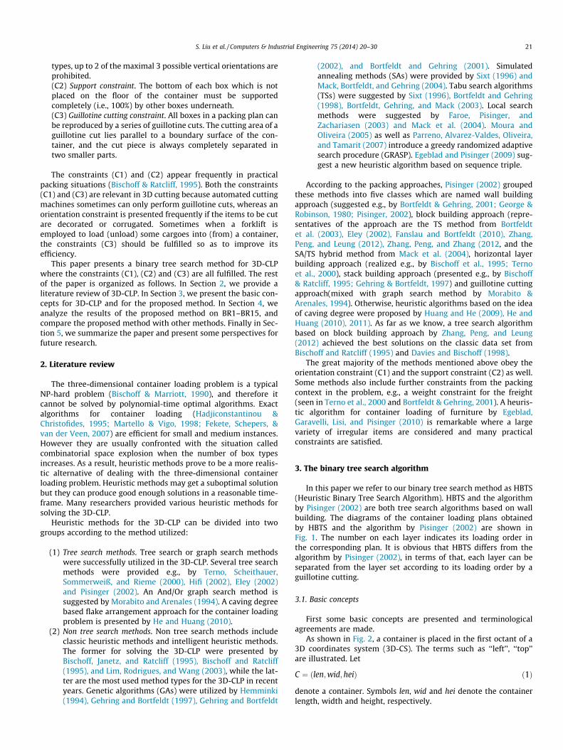
In this paper we refer to our binary tree search method as HBTS(Heuristic Binary Tree Search Algorithm). HBTS and the algorithmby Pisinger (2002) are both tree search algorithms based on wallbuilding. The diagrams of the container loading plans obtainedby HBTS and the algorithm by Pisinger (2002) are shown inFig. 1. The number on each layer indicates its loading order inthe corresponding plan. It is obvious that HBTS differs from thealgorithm by Pisinger (2002), in terms of that, each layer can beseparated from the layer set according to its loading order by aguillotine cutting.

3.1. Basic concepts

First some basic concepts are presented and terminologicalagreements are made.

As shown in Fig. 2, a container is placed in the first octant of a3D coordinates system (3D-CS). The terms such as ‘‘left’’, ‘‘top’’are illustrated. Let

C ¼ ðlen;wid; heiÞ ð1Þ

denote a container. Symbols len, wid and hei denote the containerlength, width and height, respectively.

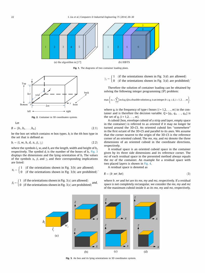
Fig. 1. The diagrams of two container loading plans.

back

z

x

y

rightleft

Top

Bottom front

hei

len

wid

o

Fig. 2. Container in 3D coordinates system.

22 S. Liu et al. / Computers & Industrial Engineering 75 (2014) 20–30

Let

B ¼ fb1; b2; . . . ; bmg ð2:1Þ

be the box set which contains m box types. bi is the ith box type inthe set that is defined as

bi ¼ ðli;wi; hi;di;ai;bi; ciÞ ð2:2Þ

where the symbols li, wi and hi are the length, width and height of bi,respectively. The symbol di is the number of the boxes of bi. Fig. 3displays the dimensions and the lying orientation of bi. The valuesof the symbols ai, bi and ci and their corresponding implicationsare listed:

ai ¼1 ðif the orientations shown in Fig: 3ðbÞ are allowedÞ0 ðif the orientations shown in Fig: 3ðbÞ are prohibitedÞ

�;

bi¼1 ðif the orientations shown in Fig: 3ðcÞ are allowedÞ0 ðif the orientations shown in Fig: 3ðcÞ are prohibitedÞ

�and;

(a)

iliw

ih

z

y

z

y

(b)

x

x

Fig. 3. An box and its lying orientat

ci ¼1 ðif the orientations shown in Fig: 3ðdÞ are allowedÞ0 ðif the orientations shown in Fig: 3ðdÞ are prohibitedÞ

�:

Therefore the solution of container loading can be obtained bysolving the following integer programming (IP) problem:

max vP ¼Xm

i¼1

liwihiqijQ is a feasible solution;qi is an integer;06qi6di;i¼1;2; . . . ;m

( );

where qi is the frequency of type-i boxes (i = 1,2, . . ., m) in the con-tainer and is therefore the decision variable. Q = {q1, q2, . . ., qm} isthe set of qi (i = 1,2, . . ., m).

A cuboid (box, envelope cuboid of a strip and layer, empty spacein the container) is referred to as oriented if it may no longer beturned around the 3D-CS. An oriented cuboid lies ‘‘somewhere’’in the first octant of the 3D-CS and parallel to its axes. We assumethat the corner nearest to the origin of the 3D-CS is the referencecorner of an oriented cuboid. The mx, my, and mz denote the threedimensions of an oriented cuboid in the coordinate directions,respectively.

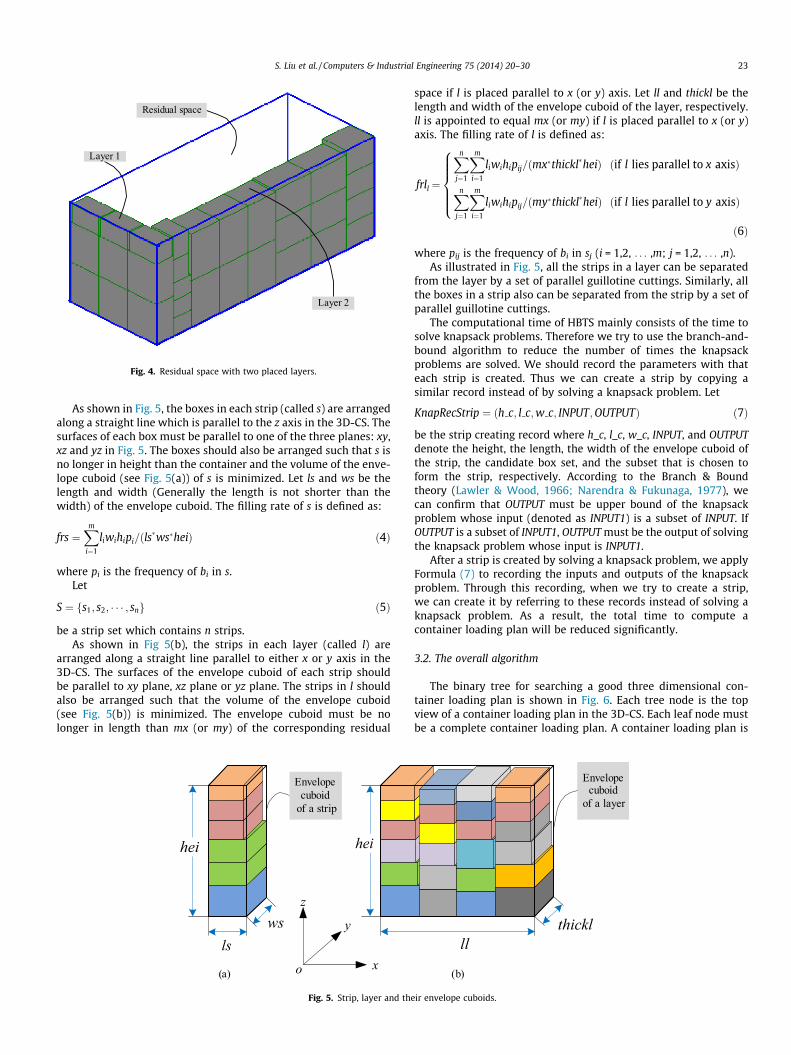
A residual space is an oriented cuboid space in the containergiven by its three side dimensions and its reference corner. Themz of each residual space in the presented method always equalsthe mz of the container. An example for a residual space withtwo placed layers is shown in Fig. 4.

A residual space is denoted as

R ¼ ðlr;wr;heiÞ ð3Þ

where lr, wr and hei are its mx, my and mz, respectively. If a residualspace is not completely rectangular, we consider the mx, my and mzof the maximum cuboid inside it as its mx, my and mz, respectively.

z

y

z

y

z

y

(c)

z

y

(d)

x x

x x

ions in 3D coordinates system.

Layer 1

Layer 2

Residual space

Fig. 4. Residual space with two placed layers.

S. Liu et al. / Computers & Industrial Engineering 75 (2014) 20–30 23

As shown in Fig. 5, the boxes in each strip (called s) are arrangedalong a straight line which is parallel to the z axis in the 3D-CS. Thesurfaces of each box must be parallel to one of the three planes: xy,xz and yz in Fig. 5. The boxes should also be arranged such that s isno longer in height than the container and the volume of the enve-lope cuboid (see Fig. 5(a)) of s is minimized. Let ls and ws be thelength and width (Generally the length is not shorter than thewidth) of the envelope cuboid. The filling rate of s is defined as:

frs ¼Xm

i¼1

liwihipi=ðls�ws�heiÞ ð4Þ

where pi is the frequency of bi in s.Let

S ¼ fs1; s2; � � � ; sng ð5Þ

be a strip set which contains n strips.As shown in Fig 5(b), the strips in each layer (called l) are

arranged along a straight line parallel to either x or y axis in the3D-CS. The surfaces of the envelope cuboid of each strip shouldbe parallel to xy plane, xz plane or yz plane. The strips in l shouldalso be arranged such that the volume of the envelope cuboid(see Fig. 5(b)) is minimized. The envelope cuboid must be nolonger in length than mx (or my) of the corresponding residual

Envelope cuboid

of a strip

hei

lsws

hei

(a)

z

xo

y

Fig. 5. Strip, layer and the

space if l is placed parallel to x (or y) axis. Let ll and thickl be thelength and width of the envelope cuboid of the layer, respectively.ll is appointed to equal mx (or my) if l is placed parallel to x (or y)axis. The filling rate of l is defined as:

frll ¼

Xn

j¼1

Xm

i¼1

liwihipij=ðmx�thickl�heiÞ ðif l lies parallel to x axisÞ

Xn

j¼1

Xm

i¼1

liwihipij=ðmy�thickl�heiÞ ðif l lies parallel to y axisÞ

8>>>><>>>>:

ð6Þ

where pij is the frequency of bi in sj (i = 1,2, . . . ,m; j = 1,2, . . . ,n).As illustrated in Fig. 5, all the strips in a layer can be separated

from the layer by a set of parallel guillotine cuttings. Similarly, allthe boxes in a strip also can be separated from the strip by a set ofparallel guillotine cuttings.

The computational time of HBTS mainly consists of the time tosolve knapsack problems. Therefore we try to use the branch-and-bound algorithm to reduce the number of times the knapsackproblems are solved. We should record the parameters with thateach strip is created. Thus we can create a strip by copying asimilar record instead of by solving a knapsack problem. Let

KnapRecStrip ¼ ðh c; l c;w c; INPUT;OUTPUTÞ ð7Þ

be the strip creating record where h_c, l_c, w_c, INPUT, and OUTPUTdenote the height, the length, the width of the envelope cuboid ofthe strip, the candidate box set, and the subset that is chosen toform the strip, respectively. According to the Branch & Boundtheory (Lawler & Wood, 1966; Narendra & Fukunaga, 1977), wecan confirm that OUTPUT must be upper bound of the knapsackproblem whose input (denoted as INPUT1) is a subset of INPUT. IfOUTPUT is a subset of INPUT1, OUTPUT must be the output of solvingthe knapsack problem whose input is INPUT1.

After a strip is created by solving a knapsack problem, we applyFormula (7) to recording the inputs and outputs of the knapsackproblem. Through this recording, when we try to create a strip,we can create it by referring to these records instead of solving aknapsack problem. As a result, the total time to compute acontainer loading plan will be reduced significantly.

3.2. The overall algorithm

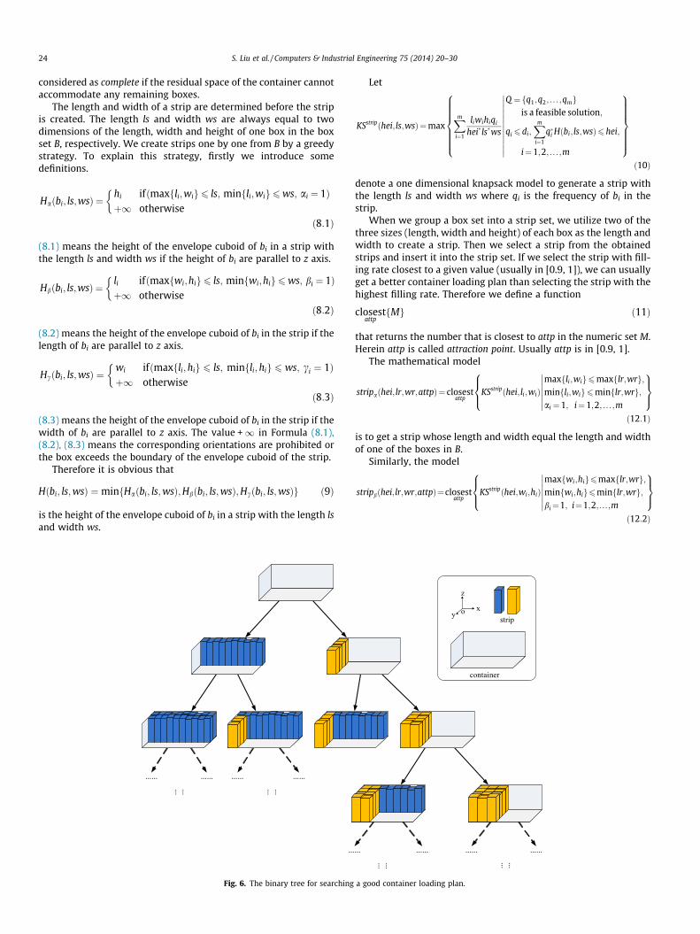
The binary tree for searching a good three dimensional con-tainer loading plan is shown in Fig. 6. Each tree node is the topview of a container loading plan in the 3D-CS. Each leaf node mustbe a complete container loading plan. A container loading plan is

Envelope cuboid

of a layer

llthickl

(b)

ir envelope cuboids.

24 S. Liu et al. / Computers & Industrial Engineering 75 (2014) 20–30

considered as complete if the residual space of the container cannotaccommodate any remaining boxes.

The length and width of a strip are determined before the stripis created. The length ls and width ws are always equal to twodimensions of the length, width and height of one box in the boxset B, respectively. We create strips one by one from B by a greedystrategy. To explain this strategy, firstly we introduce somedefinitions.

Haðbi; ls;wsÞ ¼hi ifðmaxfli;wig6 ls; minfli;wig6ws; ai ¼ 1Þþ1 otherwise

�ð8:1Þ

(8.1) means the height of the envelope cuboid of bi in a strip withthe length ls and width ws if the height of bi are parallel to z axis.

Hbðbi; ls;wsÞ ¼li ifðmaxfwi;hig6 ls; minfwi;hig6ws; bi ¼ 1Þþ1 otherwise

�ð8:2Þ

(8.2) means the height of the envelope cuboid of bi in the strip if thelength of bi are parallel to z axis.

Hcðbi; ls;wsÞ ¼wi ifðmaxfli;hig 6 ls; minfli; hig 6 ws; ci ¼ 1Þþ1 otherwise

�ð8:3Þ

(8.3) means the height of the envelope cuboid of bi in the strip if thewidth of bi are parallel to z axis. The value +1 in Formula (8.1),(8.2), (8.3) means the corresponding orientations are prohibited orthe box exceeds the boundary of the envelope cuboid of the strip.

Therefore it is obvious that

Hðbi; ls;wsÞ ¼minfHaðbi; ls;wsÞ;Hbðbi; ls;wsÞ;Hcðbi; ls;wsÞg ð9Þ

is the height of the envelope cuboid of bi in a strip with the length lsand width ws.

Fig. 6. The binary tree for searching

Let

KSstripðhei; ls;wsÞ ¼maxXm

i¼1

liwihiqi

hei�ls�ws

Q ¼fq1;q2; . . . ;qmgis a feasible solution;

qi 6 di;Xm

i¼1

q�i Hðbi; ls;wsÞ6hei;

i¼1;2; . . . ;m

������������

8>>>>>><>>>>>>:

9>>>>>>=>>>>>>;ð10Þ

denote a one dimensional knapsack model to generate a strip withthe length ls and width ws where qi is the frequency of bi in thestrip.

When we group a box set into a strip set, we utilize two of thethree sizes (length, width and height) of each box as the length andwidth to create a strip. Then we select a strip from the obtainedstrips and insert it into the strip set. If we select the strip with fill-ing rate closest to a given value (usually in [0.9, 1]), we can usuallyget a better container loading plan than selecting the strip with thehighest filling rate. Therefore we define a function

closestattp

fMg ð11Þ

that returns the number that is closest to attp in the numeric set M.Herein attp is called attraction point. Usually attp is in [0.9, 1].

The mathematical model

stripaðhei; lr;wr;attpÞ¼ closestattp

KSstripðhei; li;wiÞmaxfli;wig6maxflr;wrg;minfli;wig6minflr;wrg;ai ¼1; i¼1;2; . . . ;m

�������8><>:

9>=>;

ð12:1Þ

is to get a strip whose length and width equal the length and widthof one of the boxes in B.

Similarly, the model

stripbðhei;lr;wr;attpÞ¼closestattp

KSstripðhei;wi;hiÞmaxfwi;hig6maxflr;wrg;minfwi;hig6minflr;wrg;bi¼1; i¼1;2;...;m

�������8><>:

9>=>;

ð12:2Þ

a good container loading plan.

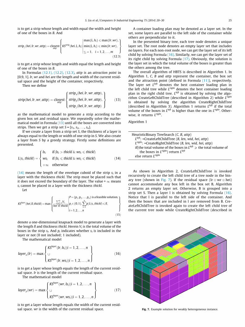
Fig. 7. Example solution for weakly heterogeneous instance.

S. Liu et al. / Computers & Industrial Engineering 75 (2014) 20–30 25

is to get a strip whose length and width equal the width and heightof one of the boxes in B. And

stripcðhei; lr;wr;attpÞ ¼ closestattp

KSstripðhei; li;hiÞ

maxfli;hig6maxflr;wrg;

minfli;hig6minflr;wrg;

ci ¼ 1; i¼ 1;2; . . . ;m

��������

8>><>>:

9>>=>>;

ð12:3Þ

is to get a strip whose length and width equal the length and heightof one of the boxes in B.

In Formulas (12.1), (12.2), (12.3), attp is an attraction point in[0.9, 1]. lr, wr and hei are the length and width of the current resid-ual space and the height of the container, respectively.

Then we define

stripðhei; lr;wr; attpÞ ¼ closestattp

stripaðhei; lr;wr; attpÞ;

stripbðhei; lr;wr; attpÞ;

stripcðhei; lr;wr; attpÞ

8>><>>:

9>>=>>; ð13Þ

as the mathematical model to generate a strip according to thegiven box set and residual space. We repeatedly solve the mathe-matical model in Formula (13) until all the boxes are converted intostrips. Then we get a strip set S = {s1, s2, . . ., sn}.

If we create a layer from a strip set S, the thickness of a layer isalways equal to the length or width of one strip in S. We also createa layer from S by a greedy strategy. Firstly some definitions arepresented.

Lðsi; thicklÞ ¼

lsi ifðlsi > thickl & wsi 6 thicklÞ

wsi ifðlsi 6 thickl & wsi 6 thicklÞ

þ1 otherwise

8>><>>: ð14Þ

(14) means the length of the envelope cuboid of the strip si in alayer with the thickness thickl. The strip must be placed such thatit does not exceed the boundary of the layer. The value +1 meanssi cannot be placed in a layer with the thickness thickl.

Let

KSlayerðhei; ll;thicklÞ¼maxPn

i¼1Vi

hei�ll�thickl

P¼fp1;p2; . . . ;png is a feasible solution;

pi 2f0;1g;Xn

i¼1

p�i Lðsi;thicklÞ6 ll;

i¼1;2; . . . ;n

���������

8>>><>>>:

9>>>=>>>;

ð15Þ

denote a one-dimensional knapsack model to generate a layer withthe length ll and thickness thickl. Herein Vi is the total volume of theboxes in the strip si. And pi indicates whether si is included in thelayer or not (0 not included; 1 included).

The mathematical model

layerxðlrÞ ¼ max

KSlayerðlr; lsiÞji ¼ 1;2; . . . ; n

[

KSlayerðlr;wsiÞji ¼ 1;2; . . . ; n

8>><>>:

9>>=>>; ð16Þ

is to get a layer whose length equals the length of the current resid-ual space. lr is the length of the current residual space.

The mathematical model

layeryðwrÞ ¼ max

KSlayerðwr; lsiÞji ¼ 1;2; . . . ; n

[

KSlayerðwr;wsiÞji ¼ 1;2; . . . ;n

8>><>>:

9>>=>>; ð17Þ

is to get a layer whose length equals the width of the current resid-ual space. wr is the width of the current residual space.

A container loading plan may be denoted as a layer set. In theset, some layers are parallel to the left side of the container whileothers are perpendicular to it.

In the presented binary tree, each tree node denotes a uniquelayer set. The root node denotes an empty layer set that includesno layers. For each non-root node, we can get the layer set of its leftchild by solving Formula (16). Similarly, we can get the layer set ofits right child by solving Formula (17). Obviously, the solution isthe layer set in which the total volume of the boxes is greater thanthe others among the tree.

The overall algorithm of HBTS is described in Algorithm 1. InAlgorithm 1, C, B and attp represent the container, the box setand the attraction point (defined in Formula (11)), respectively.The layer set Lleft denotes the best container loading plan inthe left child tree while Lright denotes the best container loadingplan in the right child tree. Lleft is obtained by solving the algo-rithm CreateLeftChildTree (described in Algorithm 2) while Lright

is obtained by solving the algorithm CreateRightChildTree(described in Algorithm 3). Algorithm 1 returns Lleft if the totalvolume of the boxes in Lleft is higher than the one in Lright. Other-wise, it returns Lright.

Algorithm 1

HeuristicBinary TreeSearch (C, B, attp)Lleft: =CreateLeftChildTree (B, len, wid, hei, attp)Lright: =CreateRightChildTree (B, len, wid, hei, attp)if(the total volume of the boxes in Lleft P the total volume of

the boxes in Lright) return Lleft

else return Lright

As shown in Algorithm 2, CreateLeftChildTree is invokedrecursively to create the left child tree of a tree node in the bin-ary tree (shown in Fig. 7). If the residual space (lr �wr � hei)cannot accommodate any box left in the box set B, Algorithm2 returns an empty layer set. Otherwise, B is grouped into astrip set S. Then a layer l is obtained by solving Formula (16).Notice that l is parallel to the left side of the container. Andthen the boxes that are included in l are removed from B. Cre-ateLeftChildTree is invoked again to create the left child tree ofthe current tree node while CreateRightChildTree (described in

26 S. Liu et al. / Computers & Industrial Engineering 75 (2014) 20–30

Algorithm 3) is invoked to create the right child tree. In the end,Algorithm 2 returns the layer set where the total volume of theboxes is the highest in the left child tree of the current treenode.

Algorithm 2

CreateLeftChildTree (B, lr, wr, hei, attp)if(B contains boxes that can be accommodated by the

residual space (lr � wr � hei))S: =CreateStripSet (B, lr, wr, hei, attp) //create a strip set

from the box set Bl: =solve Formula (16) with the strip set S and the layer

length lrremove the boxes which are included in l from BLleft: =l + CreateLeftChildTree(B, lr, wr � l.thickl, hei, attp)Lright: =l + CreateRightChildTree(B,lr,wr � l.thickl,hei,attp)

if(the total volume of the boxes in Lleft P the totalvolume of the boxes in Lright) return Lleft

else return Lright

else return £

CreateRightChildTree (see Algorithm 3) is invoked recursively tocreate the right child tree of a tree node in the binary tree (shownin Fig. 7). If the residual space (lr �wr � hei) cannot accommodateany box in the box set B, Algorithm 3 returns an empty layer set.Otherwise, B is firstly grouped into a strip set S. Then a layer l isobtained by solving Formula (17). Notice that l is perpendicular tothe left side of the container. And then the boxes that are includedin l are removed from B. CreateRightChildTree is invoked again tocreate the right child tree of the current tree node while CreateLeft-ChildTree (described in Algorithm 2) is invoked to create the leftchild tree. At last Algorithm 3 returns the layer set where the totalvolume of the boxes is the highest in the right child tree of the cur-rent tree node.

Algorithm 3

CreateRightChildTree (B, lr, wr, hei, attp)if(B contains boxes that can be accommodated by the

residual space (lr � wr � hei))S: =CreateStripSet (B, lr, wr, hei, attp) //create a strip set

from the box set Bl: =solve Formula (17) with the strip set S and the layer

length wrremove the boxes which are included in l from BLleft: =l + CreateLeftChildTree(B, lr � l.thickl, wr, hei, attp)Lright: =l + CreateRightChildTree(B, lr � l.thickl, wr, hei, attp)if(the total volume of the boxes in Lleft P the total volume

of the boxes in Lleft) return Lright

else return Lright

else return £

Algorithm 4 describes how to create a strip set from a box set B.Firstly an empty strip set S is created. Then we judge whether B con-tains boxes that can be accommodated by the residual space(lr � wr � hei). If B contains such boxes, a strip s will be createdfrom B by referring to a similar record or solving Formula (13). Thenthe boxes which are included in s will be removed from B. After that,s will be inserted into S. We repeat creating strips until B containsno boxes that can be accommodated by the residual space.

Algorithm 4

CreateStripSet (B, lr, wr, hei, attp)S: =£

while(B contains boxes that can be accommodated by theresidual space (lr � wr � hei))

B_1: =GetSimilarKnapsackRecord (hei, lr, wr, B)if(B_1 = �)

s: =solve Formula (13) with Bstore hei, lr, wr, B and the set of boxes in s as a stripcreating record in the memory

elses: =create a strip with B_1

remove the boxes which are included in s from BS: =S + s

return S

Algorithm 5 seeks a similar strip creating record from the strip cre-ation history. The similar record describes input and output of solv-ing one knapsack problem which are defined as INPUT and OUTPUTin Formula (7) and (8), respectively. We will create a strip from thebox set IN. If the height, length and width of a strip that was createdbefore are equal to hei, l and w, respectively, and IN is a subset of thecorresponding input INPUT, we get the upper bound—thecorresponding output OUTPUT. If OUTPUT is a subset of IN, we geta feasible solution—OUTPUT. It is obvious OUTPUT is the bestsolution.

Algorithm 5

GetSimilarKnapsackRecord (hei, l, w, IN)for each record(formatted as KnapRecStrip) r in the memory

if r:h c ¼ hei and r:l c ¼ l and r:w c ¼ w andr:INPUT � IN and r:OUTPUT # IN

� �return r.OUTPUT

return £

4. Computational experiments and results

The proposed HBTS algorithm is implemented in C#, and run ona server with Intel Core2 Duo Q8300@2.5 GHz and Microsoft Win-dows XP Professional. The compiling environment is MicrosoftVisual Studio 2005. By computational experiments, we find thatwe can get a good balance between the solution quality and thecomputation time if we use ATTP ¼ fattpi ¼ 0:9þ 0:003i;i ¼ 1;2; . . . ;33g as the attraction point set in the proposed algo-rithm. Algorithm 1 is invoked 33 times with attpi (i = 1, 2, . . ., 33)as the corresponding parameter. For each instance, the solutionis the best result among the 33 tested groups. Solving the knapsackproblems in Algorithm 4 consumes most of the computationaltimes. Thus a strip creating record set is generated to store theinput and output data of the knapsack functions. The frequencyof solving the knapsack problems is greatly reduced by creatingstrip according to the historic data. When the computational timeof Algorithm 1 exceeds 600 s, Algorithm 1 will terminate andreturn the best found solution.

The test data that comes from Bischoff and Ratcliff (1995) andDavies and Bischoff (1998) include 16 cases from BR0 to BR15.Each case includes 100 instances. These instances can be down-loaded from OR-Library (http://people.brunel.ac.uk/~mastjjb/jeb/

Fig. 8. Example solution for strongly heterogeneous instance.

Table 1Platforms for testing HBTS and other algorithms.

Algorithm Platform

H_BR (Bischoff & Ratcliff, 1995) –GA_GB (Gehring & Bortfeldt, 1997) Pentium 130PTSA (Bortfeldt et al., 2003) Pentium 2 GHzGRASP (Moura & Oliveira, 2005) –MSA (Parreno et al., 2007) Pentium Mobile 1500 MHz, 512 MB

Ram, C++HSA (Zhang et al., 2009) Core 2 Duo 2.0 GHz, C++A2 (Huang & He, 2009) 1.7 GHz, Windows, JavaVNS (Parreno et al., 2010) Pentium Mobile 1500 MHz, 512 MB

Ram, C++CLTRS (Fanslau & Bortfeldt, 2010) Set A: 2.6 GHz; set B: 800 MHzFDA (He & Huang, 2011) Xeon 2.33 GHz, Java, J2SE V1.5.0_14MLHS (Zhang, Peng, & Leung, 2012;

Zhang, Peng, & Zhang, 2012)Xeon X5460@3.16 GHz, DebianLinux, C++, gcc 4.3.2

HBMLS (Zhang, Peng, & Leung, 2012;Zhang, Peng, & Zhang, 2012)

Xeon X5460@3.16 GHz, DebianLinux, C++, gcc 4.3.2

HBTS Core2 Q8300@2.5 GHz, WindowsXP, C#, visual studio 2005

S. Liu et al. / Computers & Industrial Engineering 75 (2014) 20–30 27

orlib/thpackinfo.html). The numbers of box types in the 16 casesare 1, 3, 5, 8, 10, 12, 15, 20, 30, 40, 50, 60, 70, 80, 90, and 100,respectively. The box sets in from BR0 to BR15 vary from homoge-neous through weakly heterogeneous to strongly heterogeneous.

Table 2Results of HBTS and other methods for BR1–BR7.

Algorithm Constraint Filling rate (%)

BR1 BR2 B

H_BR C1&C2 85.40 86.25 8GA_GB C1&C2 85.80 87.26 8PTSA C1&C2 93.52 93.77 9GRASP C1 93.52 93.77 9MSA C1 93.85 94.22 9HSA C1&C2 93.81 93.94 9A2 C1 – –VNS C1 94.93 95.19 9CLTRS C1 95.05 95.39 9

C1&C2 94.50 94.67 9FDA C1 92.92 93.93 9MLHS C1 94.92 95.48 9

C1&C2 94.49 94.89 9HBMLS C1 94.92 95.48 9

C1&C2 94.43 94.87 9HBTS C1,C2&C3 90.57 91.46 9

Usually the instances from BR1 to BR7 are considered as weaklyheterogeneous loading problems, while the instances from BR8to BR15 are considered as strongly ones.

The instances from BR1 to BR7 were tested in H_BR (by Bischoff& Ratcliff, 1995), GA_GB (by Gehring & Bortfeldt, 1997), PTSA (byBortfeldt et al., 2003), GRASP (by Moura & Oliveira, 2005), MFB(by Lim, Rodrigues, & Yang, 2005), RHA (by Juraitis, Stonys,Starinskas, Jankauskas, & Rubliauskas, 2006), H_B (by Bischoff,2006) and SPBBL-CC4 (by Bortfeldt & Mack, 2007) which aredevoted into the weakly heterogeneous loading problem.

MSA (by Parreno et al., 2007), HSA (by Zhang, Peng, Zhu, & Chen,2009), VNS (by Parreno, Alvarez-Valdes, Oliveira, & Tamarit, 2010),CLTRS (by Fanslau & Bortfeldt, 2010), FDA (by He & Huang, 2011),MLHS (by Zhang, Peng, & Zhang, 2012), and HBMLS (by Zhang,Peng, & Leung, 2012) tested all the instances from BR1 to BR15while A2 (by Huang & He, 2009) tested the ones from BR8 to BR15.

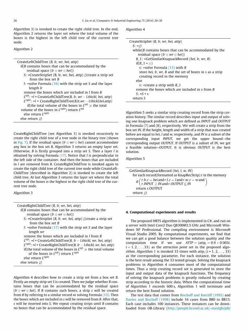
All the above algorithms fulfilled the orientation constraint(C1). Some of them fulfilled both the support constraint (C2) andthe orientation constraint (C1). The computational results listedlater come from aforementioned literatures. All the instances fromBR1 to BR15 are tested by HBTS. Both the orientation constraint(C1) and the support constraint (C2) are fulfilled in HBTS. In partic-ular, the guillotine cutting constraint (C3) is also fulfilled in HBTS(See Figs. 1, 4 and 5). The example solutions for heterogeneousinstances are illustrated in Figs. 7 and 8, respectively.

4.1. Comparison with other algorithms

Table 1 reports the platforms for testing HBTS and otheralgorithms. The data regarding other algorithms are from litera-tures cited at the beginning of this section. Some algorithms alsodescribed the platforms they used in details, while others did notreveal this information.

Table 2 reports the computational results of HBTS and otheralgorithms for the instances from BR1 to BR7. All the data in Table 2denote the average filling rate (%) for one case. HBTS is worse thanHBMLS (by Zhang, Peng, & Leung, 2012) which achieved the bestsolutions when C1 and C2 are considered. Also, HBTS is worse thanCLTRS (by Fanslau & Bortfeldt, 2010) and MLHS (by Zhang, Peng, &Zhang, 2012). The results indicate block-building approachesachieve higher volume utilization than wall-building approachesfor weakly heterogeneous instances up to now.

Table 3 reports the computational results of HBTS and otheralgorithms for BR8-BR15. All the data in Table 3 denote the averagefilling rate (%) for one case. For BR8–BR11, HBTS is worse than

R3 BR4 BR5 BR6 BR7

5.86 85.08 85.21 83.84 82.958.10 88.04 87.86 87.85 87.683.58 93.05 92.34 91.72 90.553.58 93.05 92.34 91.72 90.554.25 94.09 93.87 93.52 92.943.86 93.57 93.22 92.72 91.99– – – – –4.99 94.71 94.33 94.04 93.535.45 95.18 94.96 94.80 94.264.74 94.41 94.05 93.83 93.153.71 93.68 93.73 93.63 93.145.69 95.53 95.44 95.38 94.955.20 94.94 94.78 94.55 93.955.69 95.53 95.44 95.38 95.005.06 94.89 94.68 94.53 93.962.39 92.33 92.42 92.35 92.11

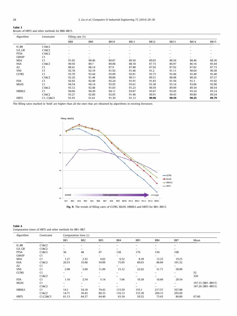
Table 3Results of HBTS and other methods for BR8–BR15.

Algorithm Constraint Filling rate (%)

BR8 BR9 BR10 BR11 BR12 BR13 BR14 BR15

H_BR C1&C2 – – – – – – – –GA_GB C1&C2 – – – – – – – –PTSA C1&C2 – – – – – – – –GRASP C1 – – – – – – – –MSA C1 91.02 90.46 89.87 89.36 89.03 88.56 88.46 88.36HSA C1&C2 90.56 89.7 89.06 88.18 87.73 86.97 86.16 85.44A2 C1 88.41 88.14 87.9 87.88 87.92 87.92 87.82 87.73VNS C1 92.78 92.19 91.92 91.46 91.2 91.11 90.64 90.38CLTRS C1 93.70 93.44 93.09 92.81 92.73 92.46 92.40 92.40

C1&C2 92.26 91.48 90.86 90.11 89.51 88.98 88.26 87.57FDA C1 92.92 92.49 92.24 91.91 91.83 91.56 91.3 91.02MLHS C1 94.54 94.14 93.95 93.61 93.38 93.14 93.06 92.90

C1&C2 93.12 92.48 91.83 91.23 90.59 89.99 89.34 88.54HBMLS C1 94.66 94.30 94.11 93.87 93.67 93.45 93.34 93.14

C1&C2 93.27 92.60 92.05 91.46 90.91 90.43 89.80 89.24HBTS C1, C2&C3 91.93 91.61 91.39 91.13 90.96 90.59 90.25 89.79

The filling rates marked in ’bold’ are higher than all the ones that are obtained by algorithms in existing literature.

Fig. 9. The trends of filling rates of CLTRS, MLHS, HBMLS and HBTS for BR1–BR15.

Table 4Computation times of HBTS and other methods for BR1–BR7.

Algorithm Constraint Computation time (s)

BR1 BR2 BR3 BR4 BR5 BR6 BR7 Mean

H_BR C1&C2 – – – – – – –GA_GB C1&C2 – – – – – – –PTSA C1&C2 36 48 97 138 179 150 198GRASP C1 – – – – – – –MSA C1 1.27 2.32 4.62 6.52 8.58 12.23 19.25HSA C1&C2 20.33 35.68 59.00 75.05 80.63 88.89 101.52A2 C1 – – – – – – –VNS C1 2.98 5.60 11.09 15.12 22.62 31.71 58.00CLTRS C1 – – – – – – – 52

C1&C2 – – – – – – – 320FDA C1 1.16 2.54 5.14 7.66 10.38 16.66 29.54MLHS C1 – – – – – – – 197.33 (BR1–BR15)

C1&C2 – – – – – – – 187.26 (BR1–BR15)HBMLS C1 14.1 34.18 79.43 115.59 155.1 217.57 327.88

C1&C2 14.71 36.43 80.33 116.13 153.38 204.15 295.69HBTS C1,C2&C3 61.13 64.37 64.40 63.34 59.52 73.63 86.80 67.60

28 S. Liu et al. / Computers & Industrial Engineering 75 (2014) 20–30

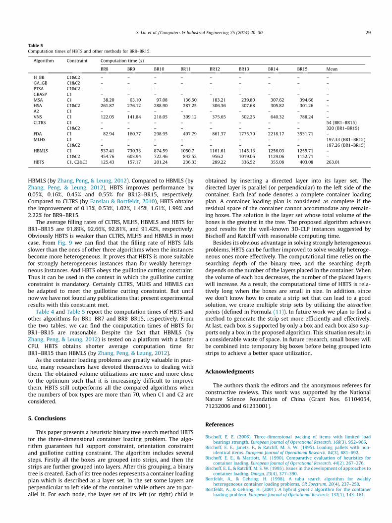
Table 5Computation times of HBTS and other methods for BR8–BR15.

Algorithm Constraint Computation time (s)

BR8 BR9 BR10 BR11 BR12 BR13 BR14 BR15 Mean

H_BR C1&C2 – – – – – – – – –GA_GB C1&C2 – – – – – – – – –PTSA C1&C2 – – – – – – – – –GRASP C1 – – – – – – – – –MSA C1 38.20 63.10 97.08 136.50 183.21 239.80 307.62 394.66 –HSA C1&C2 261.87 276.12 288.90 287.25 306.36 307.68 305.82 301.26 –A2 C1 – – – – – – – – –VNS C1 122.05 141.84 218.05 309.12 375.65 502.25 640.32 788.24 –CLTRS C1 – – – – – – – – 54 (BR1–BR15)

C1&C2 – – – – – – – – 320 (BR1–BR15)FDA C1 82.94 160.77 298.95 497.79 861.37 1775.79 2218.17 3531.71 –MLHS C1 – – – – – – – – 197.33 (BR1–BR15)

C1&C2 – – – – – – – – 187.26 (BR1–BR15)HBMLS C1 537.41 730.33 874.59 1050.7 1161.61 1145.13 1256.03 1255.71 –

C1&C2 454.76 603.94 722.46 842.52 956.2 1019.06 1129.06 1152.71 –HBTS C1, C2&C3 125.43 157.17 201.24 236.33 289.22 336.52 355.08 403.08 263.01

S. Liu et al. / Computers & Industrial Engineering 75 (2014) 20–30 29

HBMLS (by Zhang, Peng, & Leung, 2012). Compared to HBMLS (byZhang, Peng, & Leung, 2012), HBTS improves performance by0.05%, 0.16%, 0.45% and 0.55% for BR12–BR15, respectively.Compared to CLTRS (by Fanslau & Bortfeldt, 2010), HBTS obtainsthe improvement of 0.13%, 0.53%, 1.02%, 1.45%, 1.61%, 1.99% and2.22% for BR9–BR15.

The average filling rates of CLTRS, MLHS, HBMLS and HBTS forBR1–BR15 are 91.89%, 92.66%, 92.81%, and 91.42%, respectively.Obviously HBTS is weaker than CLTRS, MLHS and HBMLS in mostcase. From Fig. 9 we can find that the filling rate of HBTS fallsslower than the ones of other three algorithms when the instancesbecome more heterogeneous. It proves that HBTS is more suitablefor strongly heterogeneous instances than for weakly heteroge-neous instances. And HBTS obeys the guillotine cutting constraint.Thus it can be used in the context in which the guillotine cuttingconstraint is mandatory. Certainly CLTRS, MLHS and HBMLS canbe adapted to meet the guillotine cutting constraint. But untilnow we have not found any publications that present experimentalresults with this constraint met.

Table 4 and Table 5 report the computation times of HBTS andother algorithms for BR1–BR7 and BR8–BR15, respectively. Fromthe two tables, we can find the computation times of HBTS forBR1–BR15 are reasonable. Despite the fact that HBMLS (byZhang, Peng, & Leung, 2012) is tested on a platform with a fasterCPU, HBTS obtains shorter average computation time forBR1–BR15 than HBMLS (by Zhang, Peng, & Leung, 2012).

As the container loading problems are greatly valuable in prac-tice, many researchers have devoted themselves to dealing withthem. The obtained volume utilizations are more and more closeto the optimum such that it is increasingly difficult to improvethem. HBTS still outperforms all the compared algorithms whenthe numbers of box types are more than 70, when C1 and C2 areconsidered.

5. Conclusions

This paper presents a heuristic binary tree search method HBTSfor the three-dimensional container loading problem. The algo-rithm guarantees full support constraint, orientation constraintand guillotine cutting constraint. The algorithm includes severalsteps. Firstly all the boxes are grouped into strips, and then thestrips are further grouped into layers. After this grouping, a binarytree is created. Each of its tree nodes represents a container loadingplan which is described as a layer set. In the set some layers areperpendicular to left side of the container while others are to par-allel it. For each node, the layer set of its left (or right) child is

obtained by inserting a directed layer into its layer set. Thedirected layer is parallel (or perpendicular) to the left side of thecontainer. Each leaf node denotes a complete container loadingplan. A container loading plan is considered as complete if theresidual space of the container cannot accommodate any remain-ing boxes. The solution is the layer set whose total volume of theboxes is the greatest in the tree. The proposed algorithm achievesgood results for the well-known 3D-CLP instances suggested byBischoff and Ratcliff with reasonable computing time.

Besides its obvious advantage in solving strongly heterogeneousproblems, HBTS can be further improved to solve weakly heteroge-neous ones more effectively. The computational time relies on thesearching depth of the binary tree, and the searching depthdepends on the number of the layers placed in the container. Whenthe volume of each box decreases, the number of the placed layerswill increase. As a result, the computational time of HBTS is rela-tively long when the boxes are small in size. In addition, sincewe don’t know how to create a strip set that can lead to a goodsolution, we create multiple strip sets by utilizing the attractionpoints (defined in Formula (11)). In future work we plan to find amethod to generate the strip set more efficiently and effectively.At last, each box is supported by only a box and each box also sup-ports only a box in the proposed algorithm. This situation results ina considerable waste of space. In future research, small boxes willbe combined into temporary big boxes before being grouped intostrips to achieve a better space utilization.

Acknowledgments

The authors thank the editors and the anonymous referees forconstructive reviews. This work was supported by the NationalNature Science Foundation of China (Grant Nos. 61104054,71232006 and 61233001).

References

Bischoff, E. E. (2006). Three-dimensional packing of items with limited loadbearings strength. European Journal of Operational Research, 168(3), 952–966.

Bischoff, E. E., Janetz, F., & Ratcliff, M. S. W. (1995). Loading pallets with non-identical items. European Journal of Operational Research, 84(3), 681–692.

Bischoff, E. E., & Marriott, M. (1990). Comparative evaluation of heuristics forcontainer loading. European Journal of Operational Research, 44(2), 267–276.

Bischoff, E. E., & Ratcliff, M. S. W. (1995). Issues in the development of approaches tocontainer loading. Omega, 23(4), 377–390.

Bortfeldt, A., & Gehring, H. (1998). A tabu search algorithm for weaklyheterogeneous container loading problems. OR Spectrum, 20(4), 237–250.

Bortfeldt, A., & Gehring, H. (2001). A hybrid genetic algorithm for the containerloading problem. European Journal of Operational Research, 131(1), 143–161.

30 S. Liu et al. / Computers & Industrial Engineering 75 (2014) 20–30

Bortfeldt, A., Gehring, H., & Mack, D. (2003). A parallel tabu search algorithm forsolving the container loading problem. Parallel Computing, 29(5), 641–662.

Bortfeldt, A., & Mack, D. (2007). A heuristic for the three dimensional strip packingproblem. European Journal of Operational Research, 183(3), 1267–1279.

Bortfeldt, A., & Wäscher, G. (2013). Constraints in container loading – A state-of-the-art review. European Journal of Operational Research, 229, 1–20.

Davies, A. P., & Bischoff, E. E. (1998). Weight distribution considerations in containerloading. Technical report, Statistics and OR Group, European Business ManagementSchool. Swansea, UK: University of Wales.

Dyckhoff, H., & Finke, U. (1992). Cutting and packing in production and distribution.Heidelberg: Physica-Verlag.

Egeblad, J., Garavelli, C., Lisi, S., & Pisinger, D. (2010). Heuristics for containerloading of furniture. European Journal of Operational Research, 200, 881–892.

Egeblad, J., & Pisinger, D. (2009). Heuristic approaches for the two- and three-dimensional knapsack packing problem. Computers and Operations Research, 36,1026–1049.

Eley, M. (2002). Solving container loading problems by block arrangement.European Journal of Operational Research, 141(2), 393–409.

Fanslau, T., & Bortfeldt, A. (2010). A tree search algorithm for solving the containerloading problem. INFORMS Journal on Computing, 22(2), 222–235.

Faroe, O., Pisinger, D., & Zachariasen, M. (2003). Guided local search for three-dimensional bin-packing problem. INFORMS Journal on Computing, 15(3),267–283.

Fekete, S. P., Schepers, J., & van der Veen, J.-C. (2007). An exact algorithm for higher-dimensional orthogonal packing. Operations Research, 55, 569–587.

Gehring, H., & Bortfeldt, A. (1997). A genetic algorithm for solving the containerloading problem. International Transactions in Operational Research, 4(5–6),401–418.

Gehring, H., & Bortfeldt, A. (2002). A parallel genetic algorithm for solving thecontainer loading problem. International Transactions in Operational Research,9(4), 497–511.

George, J. A., & Robinson, D. F. (1980). A heuristic for packing boxes into a container.Computers and Operations Research, 7(3), 147–156.

Hadjiconstantinou, E., & Christofides, N. (1995). An exact algorithm for general,orthogonal, two-dimensional knapsack problems. European Journal ofOperations Research, 83, 39–56.

He, K., & Huang, W. Q. (2010). A caving degree based flake arrangement approachfor the container loading problem. Computers and Industrial Engineering, 59(2),344–351.

He, K., & Huang, W. Q. (2011). An efficient placement heuristic for three-dimensional rectangular packing. Computers and Operations Research, 38(1),227–233.

Hemminki, J. (1994). Container loading with variable strategies in each layer.Presentation, ESI-X, July 2–15, EURO Summer Institute, Jouy-En-Josas, France.

Hifi, M. (2002). Approximate algorithms for the container loading problem.International Transactions in Operational Research, 9(6), 747–774.

Huang, W. Q., & He, K. (2009). A caving degree approach for the single containerloading problem. European Journal of Operational Research, 196(1), 93–101.

Juraitis, M., Stonys, T., Starinskas, A., Jankauskas, D., & Rubliauskas, D. (2006). Arandomized heuristic for the container loading problem: Further investigations.Information Technology and Control, 35(1), 7–12.

Lawler, E. L., & Wood, D. E. (1966). Branch-and-bound methods: A survey.Operations Research, 14(4), 699–719.

Lim, A., Rodrigues, B., & Wang, Y. (2003). A multi-faced buildup algorithm for three-dimensional packing problems. Omega, 31(6), 471–481.

Lim, A., Rodrigues, B., & Yang, Y. (2005). 3-D container packing heuristics. AppliedIntelligence, 22(2), 125–134.

Mack, D., Bortfeldt, A., & Gehring, H. (2004). A parallel hybrid local search algorithmfor the container loading problem. International Transactions in OperationalResearch, 11(5), 511–533.

Martello, S., & Vigo, D. (1998). Exact solution of the two-dimensional finite binpacking problem. Management Science, 44, 388–399.

Morabito, R., & Arenales, M. (1994). An AND/OR-graph approach to the containerloading problem. International Transactions in Operational Research, 1(1), 59–73.

Moura, A., & Oliveira, J. F. (2005). A GRASP approach to the container-loadingproblem. IEEE Intelligent Systems, 20(4), 50–57.

Narendra, P. M., & Fukunaga, K. (1977). A branch and bound algorithm for featuresubset selection. IEEE Transactions on Computers, 100(9), 917–922.

Parreno, F., Alvarez-Valdes, R., Oliveira, J. F., & Tamarit, J. M. (2007). A maximal-space algorithm for the container loading problem. INFORMS Journal onComputing, 20(3), 412–422.

Parreno, F., Alvarez-Valdes, R., Oliveira, J. F., & Tamarit, J. M. (2010). Neighborhoodstructures for the container loading problem: AVNS implementation. Journal ofHeuristics, 16(1), 1–22.

Pisinger, D. (2002). Heuristics for the container loading problem. European Journal ofOperational Research, 141(2), 143–153.

Sixt, M. (1996). Dreidimensionale Packprobleme. Losungsverfahren basierend auf denMeta-Heuristiken Simulated Annealing und Tabu-Suche. Frankfurt am Main:Europaischer Verlag der Wissenschaften.

Terno, J., Scheithauer, G., Sommerweiß, U., & Rieme, J. (2000). An efficient approachfor the multi-pallet loading problem. European Journal of Operational Research,123(2), 372–381.

Wäscher, G., Haußner, H., & Schumann, H. (2007). An improved typology of cuttingand packing problems. European Journal of Operational Research, 183(3),1109–1130.

Zhang, D. F., Peng, Y., & Leung, S. C. H. (2012b). A heuristic block-loading algorithmbased on multi-layer search for the container loading problem. Computers andOperations Research, 39, 2267–2276.

Zhang, D. F., Peng, Y., & Zhang, L. L. (2012a). A multi-layer heuristic search algorithmthree dimensional container loading problem. Chinese Journal of Computers,35(12), 2553–2561.

Zhang, D. F., Peng, Y., Zhu, W. X., & Chen, H. W. (2009). A hybrid simulated annealingalgorithm for the three-dimensional packing problem. Chinese Journal ofComputers, 32(11), 2147–2156.