a tabu search procedure for multicommodity location/allocation with balancing requirements
TRANSCRIPT
Annals of Operations Research 41(1993)359-383 359
A tabu search procedure for multicommodity location/allocation with balancing requirements
Teodor G. Crainic °, Michel Gendreau, Patrick Soriano and Michel Toulouse
Centre de Recherche sur les Transports, Universit~ de Montreal, C.P. 6128, Succursale A, Montreal, Quebec, Canada H3C 3J7
Abstract
We propose a tabu search heuristic for the location/allocation problem with balancing requirements. This problem typically arises in the context of the medium term management of a fleet of containers of multiple types, where container depots have to be selected, the assignment of customers to depots has to be established for each type of container, and the interdepot container traffic has to be planned to account for differences in supplies and demands in various zones of the geographical territory served by a container shipping company. It is modeled as a mixed integer program, which combines zero-one location variables and a multicommodity network flow structure. Extensive computational results on a set of benchmark problems and comparisons with an efficient dual ascent procedure are reported. These show that tabu search is a competitive approach for this class of problems.
Keywords: Tabu search, multicommodity location/allocation problems, empty flow balancing, container transportation.
1. Introduction
These last few years have witnessed the emergence of a whole new class of optimization algorithms based on the tabu search technique. Tabu search is commonly referred to as a metaheuristic, since it is used to explore the solution space of a given problem, iteratively, with mother (or a set of other) local heuristic search procedure(s) being normally used at each step. Initially proposed by Glover [8], and independently by Hansen and Jaumard [14], tabu search has been continuously enhanced (see [6, 8-10] for the basic ingredients of the method), and applied to an increasingly wide spectrum of problems. Particularly impressive results have been obtained for hard combinatorial problems, such as quadratic programming [15], vehicle routing problems [7] and flow shop sequencing [17].
* Also at D~-partement de Sciences Administratives, Universit~ du Quebec ~t Montreal, C.P. 6192, succursale A, Montreal, Quebec, Canada H3C 4R2.
LC. Baltzer AG, Science Publishers
360 T.G. Crainic et al., Multicommodity location/allocation
Significantly less attention has been directed towards problems which display not only combinatorial characteristics, but also a strong "continuous" component. In particular, multicommodity network design problems, with, eventually, additional constraints, form such a class of models which, we believe, is a prime candidate for the successful application of tabu search based algorithms.
Such a study is of a double interest. First, these problems are "difficult" to solve, in the sense that traditional heuristics generally fail to produce optimal solutions and display significant gaps (especially when additional constraints are imposed on the multicommodity structure - see [1]), which implies that integer programming methods have to be applied. Second, the analysis of the performance of tabu search procedures in the context of problems displaying both combinatorial characteristics and a significant number of continuous variables, may help gain significant insight into the behaviour of the tabu search methodology and into ways to enhance it.
For our part, we undertake this study by focusing on a particular case of this class of problems, namely the location/allocation problem with balancing requirements. It is a problem that typically arises in the context of the medium term management of a fleet of containers of multiple types, where container depots have to be selected, the assignment of customers to depots has to be established for each type of containers, and the interdepot container traffic has to be planned to account for differences in supplies and demands in various zones of the geographical territory served by a container shipping company.
The problem is modeled as a mixed integer program, which combines zero- one location variables (and constraints) and a multicommodity network flow structure [2]. Several exact and heuristic algorithms have been developed for this formulation, in particular a very efficient dual-based procedure [4]. Given the fact that this problem is sufficiently close to general network design problems, this provides us with an ideal benchmark to critically assess the performance of tabu search procedures for this class of problems, and should allow us to build a solid methodological platform for future developments.
This paper presents a tabu search algorithm for multicommodity location problems with balancing requirements, and is organized as follows. The following section briefly describes the problem and the mixed integer formulation. It also reviews some important properties and the main algorithmic results obtained to date. Section 3 is dedicated to the detailed presentation of the tabu search procedure. Section 4 presents the computational results and analysis. We conclude by identifying future research directions.
2. Problem and model
Schematically, the problem is best described in the context of the management of a heterogeneous fleet of containers over a medium to long term planning horizon. Once a ship arrives at a port, the shipping company has to deliver loaded containers
T.G. Crainic et al., Multicommodity location~allocation 361
to their designated in-land destinations. These containers come in several types and sizes, and various transportation modes may be used to move them. Following their delivery and unloading by the importing customer, empty containers may be retumed to the depot of the port that initiated the loaded movement, or may be repositioned to a different depot in prevision of future requests for empty containers. Indeed, the same, or other, customers are also requesting containers, of specific types, for subsequent shipping of their own products. Empty containers are delivered from depots, are loaded, and are subsequently moved, by land and maritime transportation means, to their final destinations. Additionally, regional unbalances in empty container availabilities and needs throughout the network require that empty containers be shipped between depots to "balance" the network. Interdepot transportation is assumed to be more efficient, per moved unit, than movements between depots and customers, due to the larger volumes of traffic which may be consolidated for transshipment over relatively long distances.
The general problem is therefore to locate the empty container depots in order to collect the supply of empty containers available at customers' sites and to satisfy the customer requests for empty containers, while minimizing the total operation cost: the cost of opening and operating the depots, plus the transportation costs between customers and depots and the costs generated by moving empty containers among depots to "balance" the network. In practical applications, this strategic/tactical logistics problem has to be repeatedly solved since, often, container shipping companies do not build their own depots, but rather use facilities available from other modes (e.g. ports and rail yards). It is then a question of deciding which facilities to use, according to the demand and the cost structure particular to the specific planning period. Dejax et al. [5], present a full description and discussion of the problem based on an actual application of planning the land operations of a maritime container shipping company.
Let C, D and P represent the sets of customers (cardinality m), candidate depots (cardinality n), and products (cardinality p), respectively. Crainic et al. [2] model this problem as:
(P) Minimize Z= ~ fyyj + ~., { ~.~ ~.~ (ciypx~i p +cyipxjip)+ ~_~ ~.,sj~wj~,} jeD paP ieCjeD jaDkaD
subject to ~x~/p = O/p jeD
jeD
VieC, peP, (1)
xup <- Oipyj
xjip < Dipy v i c e , j e D , peP , (2)

362 T.G. Crainic et al., Multicommodity location~allocation
Z + Z Z = o iEC k~D i~C kED
V j e D , p e P , (3)
x~p >_ O
%,>.0
W jk p >. 0
V i e C , j e D , p e P , (4)
V j e D , k e D , p e P , (5)
yj ~ {0,1} Vj e D, (6)
where
y= (y?
Xij p, Xj~
wj~, wkjt,
c~jp, cjzt,
sj~, skit,
Oil, D~I,
opening vector for depots, j ~ D; Yi equals 1 if depot is open and zero otherwise;
flows (in both directions) of product p, p ~ P, between customer i, i ~ C, and depot j, j ~ D;
flows of product p, p ~ P, between depots j and k, j ~ D, k ~ D;
"fixed" cost of depot j, j ~ D;
unit transportation costs for product p, p ~ P, between customer i, i ~ C, and depot j, j ~ D;
unit transportation costs for product p, p a P, between depots j and k, j ~ D, k ~ D;
supply at node (customer) i, i e C, of product p, p ~ P;
demand at node (customer) i, i ~ C, of product p, p ~ P.
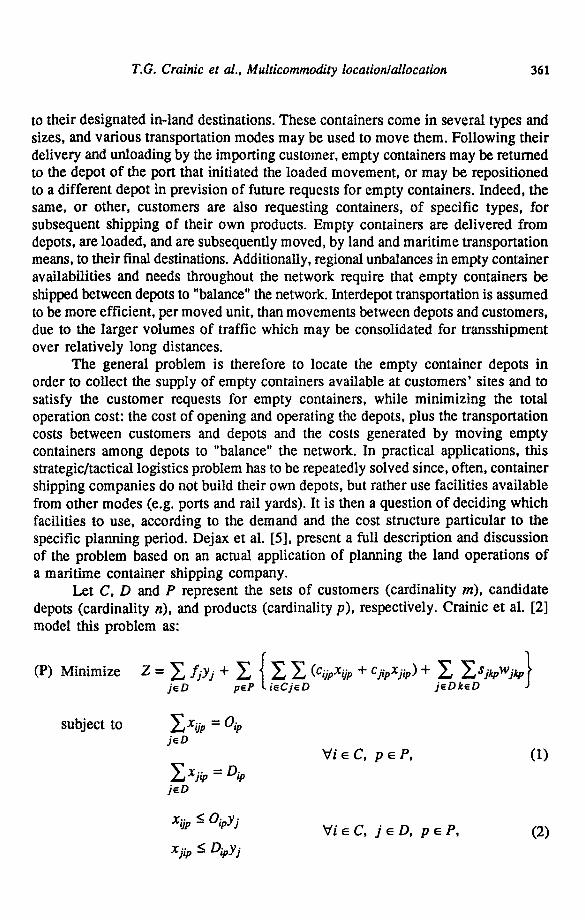
Constraints (1) ensure that demand and supply requirements are met. Constraints (2) forbid exchanges between customers and closed depots (analogous constraints for interdepot movements have been shown to be redundant if the applicable transportation costs satisfy the triangle inequality; they can thus be dropped). Constraints (3) correspond to the interdepot balancing requirements. Figure 1 illustrates the structure of the problem.
Several algorithmic developments have already been spurred by this problem. The exploration of classical heuristic approaches (greedy, interchange, etc.) has been initiated with encouraging success [12]. Lagrangian relaxation approaches have proved quite efficient for moderate size problems, but their performance seems to deteriorate with the number of commodities [12, 13]. Research is continuing in this direction, as well as in the area of primal/dual approaches [16]. Crainic et al. [3] have proposed a branch-and-bound algorithm to solve the problem exactly. In particular, they have shown that classical results for the simple plant location problem do not extend to this problem, and have developed and analyzed specific branching and bounding rules. Recently, Crainic and Delorme [4] have presented

T.G. Crainic et al., Multicommodity location~allocation 363
Supply
w ~" " . ~ - . . ~ _ ' _ . ~ - - - - - ~ " "~" Depots
X
Demands Fig. 1. Network flow structure for the problem.
Customers
Customers
an extremely efficient dual-ascent heuristic procedure. In fact, for now, this is the most efficient procedure for the multicommodity location problem with balancing requirements. Yet, most solutions display optimality gaps larger than 1% and, indeed, the procedure finds local optima for several problems. Hence, improvements are still possible and we aim at achieving some through the application of tabu search.
An important characteristic of the present formulation consists in the network structure that underlies it and which is apparent in fig. 1. This property is extensively used in the various algorithmic developments. The particular form that we will u s e
to develop the tabu search method concerns the formulation (P(y)) which results when the location variables yj are fixed to some values ~, j ~ D:
(P(y)) Minimize Z(P(.y))= ~ ( ~ ~ (CijpXij p "t" CjipXjip)"1" 2 2SjkpWjkpl pEP ~, ieCje-D jeD keD )
xiyp = Oip j sD
iEC, pEP,
j~D
364 T.G. Crainic et al., Multicommodity location~allocation
E Xijp + E WkJP- ~ X J i P - 2Wjkp = 0 i eC k E D iEC k~D
x~p, xjip >- o
W jk p >-- 0
j e D , p e P ,
i eC, j e D , p e P ,
j e D , k e D , p e P ,
where D represents the set of all open (i.e. ~ = 1) depots. We may then show that:
PROPERTY 1
(P(y)) is an uncapacitated multicommodity minimum cost network flow problem.
3. The tabu search procedure
3.1. THE SEARCH SPACE
The tabu search procedure that we propose to solve our problem exploits property 1 of the previous section. More precisely, since it is possible to obtain "optimal" values of the continuous flow variables x and w corresponding to any given vector of location variables y by solving a series of minimum cost flow problems, the search procedure can be restricted to the space of the location variables. In the following, when we refer to a "solution", this should be interpreted as an assignment of O's and l ' s to the location variables. The objective value associated with a solution y is then z ( y ) = Y~j~Dfj~ + Z(P(y)) .
Since most customers are linked to only a subset of the potential depot locations, there are customers who, in some solutions, do not have access to an open depot, thus making those solutions infeasible. In an early implementation of the algorithm, we tried restricting the search to feasible solutions, but this proved impractical, since the search space was too constrained. To circumvent this difficulty, an artificial depot was added. This depot (which is always considered to be open) is linked to all customers (but not to the other depots) by very high cost arcs. These costs are such as to guarantee that the artificial arcs will bear no flow, unless the solution is infeasible. This provides us with an easily implemented test regarding the feasibility of solutions: a solution is feasible if and only if the total flow on the artificial arcs is zero. As the search proceeds, we keep track of the feasibility of the solutions encountered to make sure that the best solution discovered is indeed feasible and to adjust some control parameters of the procedure as will be explained later on.
3.2. NEIGHBOURHOOD STRUCTURE
The basic iterative step of any tabu search procedure involves moving from a current point (solution) in the search space to one of its "neighbours" according

T.G. Crainic et al., Multicommodity locationlallocation 365
to some suitably defined neighbourhood structure. With regard to the problem at hand, a "natural" neighbourhood structure can be defined by considering moves in which a single yj variable is modified (complemented), i.e. the status of a single depot is changed (from open to closed or vice-versa). Our search procedure indeed allows for such moves: moves in which a depot is opened are called add moves, and moves in which a depot is closed are called drop moves. However, early on in the development of the procedure, it was found out that add/drop moves suffered from several disadvantages, especially when fixed costs of depots are large relative to other costs. First, with them, objective function values tend to vary wildly from one solution to the next; second, since in most problems the good solutions tend to have the same number of open depots, add/drop moves do not allow for the most efficient exploration of the solution space in the latter stages of the search.
A third type of move was therefore defined: swap moves in which we simultaneously open a depot and close another (this amounts to performing at once an add and a drop move). Since the number of possible swaps at any given time is much larger than the number of possible add/drop moves, and since swaps between depots that are far apart are generally unprofitable, it was decided to restrict swaps to pairs of depots which are physically close: for each open depot j, we only consider the closed depot k which is the "closest" (as measured by the balancing costs, i.e.Y.psj~,). A nice feature of swap moves is that they allow for an efficient implementation of search intensification strategies by keeping the number of open depots unchanged.
3.3. THE SEARCH STRATEGY
The search strategy is organized around two complementary objectives: (1) determining the optimal number of open depots, (2) for a fixed cardinality of the set of open depots, finding the best possible configuration of open depots. The first objective is accomplished by performing sequences of add and drop moves (these are called addldrop sequences) which allow for the examination of open depot sets of various sizes, while the second is pursued by consecutively executing several swap moves (thus creating swap sequences). Swap sequences are further divided into normal swap sequences and strict swap sequences. In the former, the best candidate move is always implemented, regardless of its real impact on the economic function; it can therefore be non-improving. The search resumes from this new solution. In strict swap sequences, however, we evaluate the real cost of the selected move and implement it only if it improves on the current solution. If the move is non-improving, it is not implemented and the search resumes from the same current solution.
The basic step of the search procedure consists of an add/drop sequence followed by a normal swap sequence which is initiated from the best solution found in the add/drop sequence. This combined add/drop-normal swap sequence yields a best "local" solution which is either feasible or infeasible. If it is feasible, we
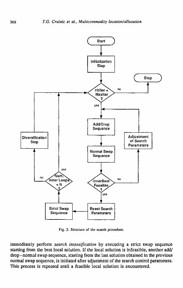
366 T.G. Crainic et al., Multicommodity location~allocation
I Diversification I Step t
Start .)
Initialization Step
~r
yes I
Add/Drop Sequence
I Norma, Swap''l Sequence I
yes ~r
r io
r io
Stop )
Adjustment of Search
Parameters
Fig. 2. Structure of the search procedure.
immediately perform search intensification by executing a strict swap sequence starting from the best local solution. If the local solution is infeasible, another add/ drop-normal swap sequence, starting from the last solution obtained in the previous normal swap sequence, is initiated after adjustment of the search control parameters. This process is repeated until a feasible local solution is encountered.
T.G. Crainic et al., Multicommodity location~allocation 367
A portion of the search beginning with an add/drop sequence and terminating with a strict swap is called an inner loop; N of these inner loops (where N is an input parameter) followed by a search diversification step (described later on) make up an outer loop.
The overall search procedure starts from an initial solution and performs a sequence of outer loops until some termination criterion is met. In the current implementation, this termination criterion is simply the total number of iterations since the beginning of the search.
The general structure of the search procedure is summarized in fig. 2.
3.4. IN1TIAL SOLUTION
The initial solution from which the search is to proceed, can be determined in several ways. The simplest one corresponds to opening all depots, i.e. setting yj = 1, V j e D. Such an initial solution has, in general, the disadvantage of being "far" from good solutions, since, in most cases, the number of open depots in these is much smaller than IDI. An immediate consequence of this situation is that the procedure has to close several depots before starting to explore interesting areas of the search space.
An altemative method for selecting an initial solution consists of first determining an estimate d (not necessarily very precise) of the number of open depots in good solutions and then opening the d depots with lowest fixed costs. This is the approach we have used in our implementation.
3.5. IMPLEMENTATION OF ADD/DROP AND SWAP SEQUENCES
The two types of sequences share a number of common features. First, at each iteration of both, only a random sample of possible moves is considered, in order to reduce the computational burden. These samples are not of fixed sizes, but are constructed using specified selection probabilities: for each possible move under the current sequence, a uniform (0, 1) random number is drawn; the move is included in the sample if this number falls below the corresponding probability. An interesting consequence of this sample building scheme with respect to add/drop sequences is that it provides a natural adjustment mechanism of the proportion of add and drop moves making up the sample: when most depots are open, the sample is mainly made up of drop moves, while the opposite is true when there are only a few open depots. We noted, however, that this procedure could, under certain circumstances, lead to situations where a sample would contain no, or almost no, moves of a given type. A minimum value of 4 was thus imposed on the number of potential add and drop moves to be included in a sample of add/drop sequences (if less than 4 moves of a given type are possible, all of them are considered).
At the beginning of the algorithm, initial values must be provided for the selection probabilities of add, drop and swap moves. These selection probabilities

368 T.G. Crainic et al., Multicommodity location/allocation
do not however remain fixed during the whole search. Indeed, these constitute an important control mechanism with regard to feasible/infeasible solutions. Since low selection probabilities tend to constrain the search, we increase the current probability values whenever a combined add/drop normal swap sequence fails to produce a feasible solution. The updating schedule is as follows: add/drop probabilities are increased by 0.08 and swap probabilities by 0.05 (up to, naturally, a maximum value of 1). To help in the search for feasible solutions, the cost values of artificial arcs are also multiplied by 2 when selection probabilities are increased. All these search control parameters are reset to their original values at the beginning of each outer loop.
Another feature shared by add/drop and swap sequences is that their length is not known beforehand: each sequence continues until a number of iterations has been performed without producing an improvement in the value of the local optimum. Add/drop and swap sequences however use distinct termination criteria (ADreps and SWreps respectively) which are specified as input parameters. It is possible to alter the behaviour of the search significantly by varying these parameters, as will be discussed in the section on computational results.
Add/drop and swap sequences both use short-term memory tabu lists. For add/drop sequences, there is one list T1 in which are recorded the 17"11 last depots added or dropped from the solution. The reverse moves are forbidden as long as the depots remain on the list. For swap sequences, a list T2, which records the most recently performed swaps as pairs of depots, is maintained. It prevents a reversal or a repetition of the IT21 last moves. It is necessary to forbid the repetition of swaps, because cycling can occur when only reversals are prohibited. For instance such as {(close Jl, open J2), (close J2, open J3), (close J3, open Jl), (close Jl, open J2) . . . . } would be legal in that case.
All short-term tabu lists are emptied at the beginning of swap sequences since these start at the best local solution (thus invalidating the recent history of the search). At the end of swap sequences, however, the information recorded in the swap tabu list is transferred to the add/drop list (each swap is then interpreted as the combination of an add and a drop move).
3.6. EVALUATION OF NEIGHBOURS
As was mentioned earlier, the computation of the exact value of the objective function associated with a given solution y involves solving the multicommodity flow problem P(y'-), or equivalently a series of single commodity minimum cost flow problem. Even if an efficient network flow code such as RNET [I 1] is used, it is extremely time-consuming to evaluate all candidate moves exactly. To alleviate this problem, we have decided to compute estimates, rather than exact values, of the objective function for all candidate moves considered. The basic principle underlying these estimates is that flow pattems should not vary very much when a single depot is opened or closed. The move to be implemented is selected on the basis of these

T.G. Crainic et al., Multicommodity location~allocation 369
estimates as the one yielding the minimum among them, and the value of the resulting solution is then computed exactly with RNET.
3.6.1. Add moves
Let ~ be a candidate solution obtained from the current solution y by opening depot j . To estimate the difference Z (~ ) - Z(y), we re-assign to depot .i every customer which is located closer (with respect to cost) to j than to the depot to which it is currently assigned under y. This will have two consequences: a decrease in customer-to-depot (and depot-to-customer) flow costs, which is easily accounted for, and a modification of the net flow balance at each depot, for each product, which will result in different flow balancing costs. Computing exactly the new flow balancing costs would involve solving for each product a classical transportation problem and is therefore not attractive. Instead, we use the following formula:
p~e k.j~D J where
b
V
is the estimate of the balancing flow costs under ~,
is the set of open depots in ~,
is the number of open depots in ~,
is the flow balance of product p at depot j, and
is an estimate of the unit balancing flow cost for product p for configurations with fl open depots.
The estimate ~'/~ can be derived from previous solutions through an exponential smoothing procedure. Let ~ be the vector of balancing flows associated with a solution y with ,6 open depots. Then the unit balancing flow costs for product p is given by
j~D k~D j~D k~D
Initially, all ~'~ are set equal to zero. The first time that a solutiony with fl open depots is visited, ~'ff is reset to ~ ( y ) , for every p. Later in the search, when other solutions y with i~ open depots are encountered, ~t~ is updated using the classical rules of exponential smoothing" (t , .= a ~ p ( y ) .[. ( 1 - a ) ~ P where ct is • # . . # /3 the smoothing constant (0 < a < 1), which is an input parameter.
3.6.2. Drop moves
The procedure for evaluating drop moves is quite similar to the previous one, except that we simply reassign to the closest open depot the customers which were
370 T.G. Crainic et al., Muhicommodity location~allocation
allocated to the depot which is to be closed if the move is executed. Note however that, in this case, customer-to-depot flow costs may increase or decrease depending on the exact configuration of the solution.
3.6.3. Swap moves
Every swap move is evaluated as the combination of a drop move followed by an add move using the procedures defined above.
3.6.4 Adjustment of balancing flow costs
During preliminary testing of the heuristic, it was found out that the estimates of balancing flow costs produced by the approximation were sometimes too optimistic (i.e. too low) in particular for the larger test problems. An adjustment factor ~7, that varies with problem size, is thus used to multiply the balancing flow cost before computing the value of the objective function estimates. In essence, this amounts to slightly penalizing solutions having strong balancing flow components in order to compensate for the underestimation of their cost.
3.7. SEARCH DIVERSIHCATION
After performing N inner loops, the search procedure is re-directed to previously unexplored portions of the search space by performing a search diversification step. This step uses a long-term memory in which we record the number of times that the status of each depot has been modified (changed from open to closed or vice-versa).
The search diversification step is always performed starting from the best global solution found up to this point in the search. Based upon the values stored in the long-term memory, the 7 depots with the lowest activity counts (number of status modifications) are selected. The status of each of these depots is then changed, providing thus a new solution which differs from the best one in exactly 7 components. To prevent too quick a reversal of these depots to their previous status, they are added to the short-term memory.
Considering the fact that values in the long-term memory tend to evolve slowly, it was felt necessary to provide a diversification memory in order to record the last set of depots that were selected for diversification. These are then excluded from consideration in the next diversification step to prevent repetitive patterns.
4. Computational results
Extensive computational testing was performed to assess the impact of parameter settings on the quality of the solutions produced by our method and to determine whether tabu search is a competitive approach for this problem when compared to more traditional heuristics such as dual ascent.
T.G. Crainic et al., Multicommodity location~allocation 371
4.1. THE PROBLEM SET
The set of benchmark problems for these tests was extracted from a much larger set of randomly generated problems that had been created previously to evaluate other solution approaches. 20 problems made up this set: 12 of these are "medium-size" problems (numbered M1 to M12) with about 25 potential depot locations and 125 customers, while the remaining 8 are "large-size" problems (numbered L1 to L8) with about 44 depot sites and 220 customers. The number of different container types ("products") ranges from 1 to 6 for the medium problems and from 1 to 2 for the large ones.
Each group of problems can be further broken into two subgroups: one with low fixed-to-variable cost ratios (M1 to M6 and L1 to L4) and the other with high ratios (M7 to M12 and L5 to L8); in fact, the problems with the high ratios were obtained from the ones with the low ratios by multiplying the depot fixed costs by 10 (for instance, problem M7 is the same as M1 except for fixed costs). The fixed- to-variable cost ratio is an important attribute of the problems, since it was known beforehand that problems with high ratios display much larger dual gaps than those with low ratios.
The last attribute of the problem is the number of "regions" that they cover. This should be interpreted as a measure of the level of imbalance in the network supply and demand for the various products: the larger this number, the higher will balancing flows between depots be. This attribute does not seem to have a large impact on the quality of the solutions, but it allows one to create problems that are not too similar.
The problem characteristics are summarized in table 1. Further details on the generation procedure for these problems can be found in [3].
4.2. EXPERIMENTATION WITH PARAMETER SETI'INGS
The experimentation on parameter settings was conducted in two phases. The first phase (preliminary testing) consisted in solving subsets of the problem set with various settings of all parameters to determine whether some of these could be fixed once and for all, either because the solution quality was insensitive to them or because some settings were obviously superior to others. At the end of this phase, it was decided to fix, for all subsequent runs, the number of iterations to 300 (longer runs seldom produced better solutions while requiring proportionally larger CPU times), the number of inner loops in an outer loop to 2, the exponential smoothing constant for unit balancing flow cost estimates a to 0.3, and the balancing flow cost adjustment factor r/ to 1 for medium problems and 1.1 for large ones. As for the number of open depots in initial solutions, it was set to 5 for medium-sized problems with high costs (M7-M12), to 10 for medium problems with low fixed costs (M1-M6) and for large problems with high fixed costs (L5-L8) , and to 15 for large problems with low fixed costs (L1-L4).

372 T.G. Crainic et al., Multicommodity location/allocation
Table l
Test problem characteristics.
Depot Level of Problem Customers candidates Regions Products fixed costs
M1 125 25 1 1 Low M2 125 25 1 4 Low M3 124 26 2 3 Low M4 125 25 2 6 Low MS 124 26 4 1 LOw M6 124 26 4 4 LOw M7 125 25 1 1 High M8 125 25 1 4 High M9 124 26 2 3 High
M10 125 25 2 6 High Mll I24 26 4 1 High M12 124 26 4 4 High L1 219 44 1 1 Low L2 219 44 1 2 Low I_3 220 43 3 1 LOw IA 219 44 3 2 Low I.,5 219 44 1 1 High I.,6 219 44 1 2 High L7 220 43 3 1 High I.,8 219 44 3 2 High
The second phase of parameter setting experimentation (systematic testing) involved solving the whole problem set repeatedly, while varying one or two parameters and keeping the others fixed. It should be noted that, given the limited number o f test problems, it is impossible to draw statistically valid conclusions from these results. The aim of the following discussion is thus to provide some guidelines for parameter setting in our problem context.
4.2.1. Tabu list length and number of iterations without improvement
The first obvious candidates for systematic testing are the length of the two short-term tabu lists. However, considering the fact that there might be a strong interaction between the length of tabu list and the number of iterations without improvement that are allowed in a given sequence (since tabu lists are an anti- cycling device), it was deemed necessary to vary, for each type of sequence, these two parameters together.
Three lengths were considered for the tabu lists: 2, 5 and 8 (preliminary testing had shown that larger list sizes were inefficient). For each list size, three values of the number o f iterations without improvement (called "repetitions" in the following and in the tables) were examined; these correspond to ratios of repetitions
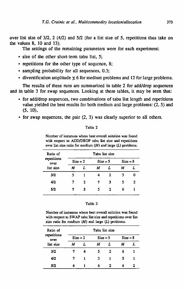
T.G. Crainic et al., Multicommodity location~allocation 373
over list size of 3/2, 2 (4/2) and 5/2 (for a list size of 5, repetitions thus take on the values 8, 10 and 13).
The settings of the remaining parameters were for each experiment:
• size of the other short-term tabu list, 5;
• repetitions for the other type of sequence, 8;
• sampling probability for all sequences, 0.3;
• diversification amplitude ~, 6 for medium problems and 12 for large problems.
The results of these runs are summarized in table 2 for add/drop sequences and in table 3 for swap sequences. Looking at these tables, it may be seen that:
• for add/drop sequences, two combinations of tabu list length and repetitions value yielded the best results for both medium and large problems: (2, 5) and (5, 10),
• for swap sequences, the pair (2, 3) was clearly superior to all others.
Table 2
Number of instances where best overall solution was found with respect to ADD/DROP tabu list size and repetitions over list size ratio for medium (M) and large (L) problems.
Ratio of repetitions
o v e r
list size
Tabu list size
Size = 2 Size = 5 Size = 8
M L M L M L
3/2 5 1 4 2 3 0
4/2 7 2 7 3 5 2
5/2 7 3 5 2 6 1
Table 3
Number of instances where best overall solution was found with respect to SWAP tabu list size and repetitions over list size ratio for medium (M) and large (L) problems.
Ratio of Tabu list size repetitions
Size = 2 Size = 5 Size = 8 o v e r
list size M L M L M L
3/2 7 4 5 2 6 1
4/2 7 1 3 1 5 1
5/2 6 1 6 2 4 2
374 T.G. Crainic et al., Multicommodity location/allocation
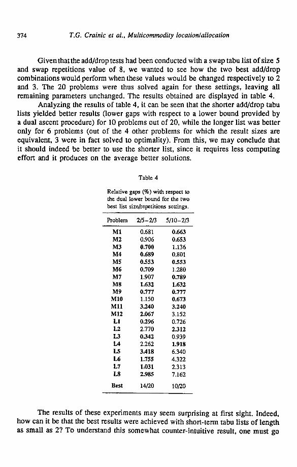
Given that the add/drop tests had been conducted with a swap tabu list of size 5 and swap repetitions value of 8, we wanted to see how the two best add/drop combinations would perform when these values would be changed respectively to 2 and 3. The 20 problems were thus solved again for these settings, leaving all remaining parameters unchanged. The results obtained are displayed in table 4.
Analyzing the results of table 4, it can be seen that the shorter add/drop tabu lists yielded better results (lower gaps with respect to a lower bound provided by a dual ascent procedure) for 10 problems out of 20, while the longer list was better only for 6 problems (out of the 4 other problems for which the result sizes are equivalent, 3 were in fact solved to optimality). From this, we may conclude that it should indeed be better to use the shorter list, since it requires less computing effort and it produces on the average better solutions.
Table 4
Relative gaps (%) with respect to the dual lower bound for the two best list size/repetitions settings.
Problem 2/5-2/3 5/10-2/3
M1 0.681 0.663 M2 0.906 0.653 M3 0.700 1.136 M4 0.689 0.801 M5 0.553 0.553 M6 0.709 1.280 M7 1.907 0.789 M8 1.632 1.632 M9 0.777 0.777
MIO 1.150 0.673 MI1 3.240 3.240 M12 2.067 3.152 L1 0.296 0.726 L2 2.770 2.312 L3 0342 0.939 IA 2.262 1.918 1,5 3.418 6.340 L6 1.755 4.322 L7 1.031 2.313 L8 2.985 7.162
Best 14/20 10/20
The results of these experiments may seem surprising at first sight. Indeed, how can it be that the best results were achieved with short-term tabu lists of length as small as 2? To understand this somewhat counter-intuitive result, one must go

T.G. Crainic et al., Multicommodity location~allocation 375
back to the overall organization of the search procedure. Shorter list lengths together with low repetition values imply that each sequence in the search is fairly short and that the search process thus alternates between the two types of sequences. This, in turn, may help directing the search to the most promising regions of the solution space. Finally, another factor must be taken into account. Since the number of inner loops per outer loop is fixed, shorter sequences result in shorter inner loops, which means that diversification is performed more often. This by itself allows for the exploration of a larger portion of the solution space.
4.2.2. Sampling probabilities The next series of experiments involved changing the sampling probabilities
for both add/drop and swap moves. These were modified simultaneously, since it was felt that both probabilities would have a similar impact on the performance of the method. Three different probability levels were considered: 0.3, 0.5 and 0.7. The best values for tabu list lengths and repetitions were used and all other parameters were left unchanged. The results obtained are displayed in table 5.
Table 5
Influence of sampling probabilities on relative gap (%).
Problem 0.3 0.5 0.7
M1 0.681 0.663 0.663 M2 0.906 0.619 0.879 M3 0.700 1.276 0.844 M4 0.689 0.567 0.751 M5 0.553 0.553 0.553 M6 0.709 0.938 0.572 M7 1.907 0.789 0.789 M8 1.632 1.813 1.632 M9 0,777 0.777 0.777 M10 1.150 0.999 0.673 M l l 3.240 3.240 3.240 M12 2.067 2.339 3.848 L1 0.296 0.296 0.296 L2 2.770 1.977 2.133 [,3 0.342 0A01 0.330 1,4 2.262 2.028 1.821 L5 3A 18 3.332 3.332 L6 1.755 2.222 3.749 L7 1.031 1.860 1.860 L8 2.985 3.856 5.193
Best 1020 10/20 12/20
376 T.G. Crainic et al., Multicommodity location~allocation
These results show that, in general, sampling probabilities have a very small impact on the quality of the solution. However, this statement must be qualified, Preliminary testing with very low sampling probabilities such as 0.1 had yielded notably inferior solutions. It would be more correct to state that 0.3 is a sampling probability value large enough for the method to perform adequately and that there are no significant gains to be made by using larger values (this only increases CPU time needlessly).
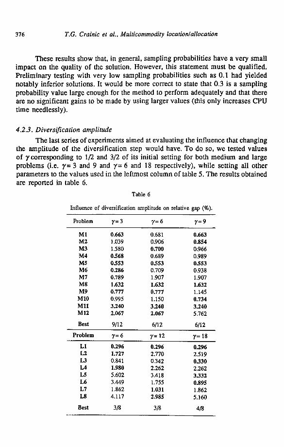
4.2.3. Diversification amplitude The last series of experiments aimed at evaluating the influence that changing
the amplitude of the diversification step would have. To do so, we tested values of 7corresponding to 1/2 and 3/2 of its initial setting for both medium and large problems (i.e. 7= 3 and 9 and 7 = 6 and 18 respectively), while setting all other parameters to the values used in the leftmost column of table 5. The results obtained are reported in table 6.
Table 6
Influence of diversification amplitude on relative gap (%).
Problem 7 = 3 7 = 6 7 = 9
M 1 0.663 0.681 0.663 M2 1.039 0.906 0.854 M3 1-580 0.700 0;966 M4 0.568 0.689 0.989 M5 0.553 0.553 0.553 M6 0.286 0.709 0.938 M7 0.789 1.907 1.907 M8 1.632 1.632 1.632 M9 0.777 0.777 1.145 M10 0.995 1.150 0.734 M l l 3.240 3.240 3.240 M12 2.067 2.067 5.762
Best 9/12 6/12 6/12
Problem 7= 6 y= 12 7= 18
L1 0`296 0.296 0.296 L2 1.727 2.770 2_519 L3 0.841 0.342 0.330 L4 1.980 2.262 2.262 L5 5.602 3.418 3.332 L6 3.449 1.755 0.895 L7 1.862 1.031 1.862 L8 4.117 2.985 5.160
Best 3/8 3/8 4/8
T.G. Crainic et al., Multicommodity location/allocation 377
Analyzing the results of table 6, one may observe that for medium problems the smallest value of 7 ( 7 = 3) yielded the best results. For large problems, all 3 settings of 7provided similar results on the average. However, if one is concerned with the robustness of the method, the value of 7 to be preferred here is 12, since large gaps (> 5%) were sometimes obtained with the other two settings (e.g. problems L5 and L8).
4.3. COMPARISON WITH DUAL ASCENT
In order to assess the competitiveness of tabu search for this type of problem, we compared our results with those obtained by the dual ascent heuristic developed by Crainic and Delorme [4]. This procedure has been proven to be very effective and extremely quick on a large set of test problems (which included our benchmark problems), and was therefore an obvious candidate for comparison.
In addition, we also implemented a straightforward descent procedure to be run from the solution provided by the tabu search algorithm upon its completion. The motivation behind this idea is the following. In the tabu search procedure, we only compute approximate values when evaluating candidate moves and, moreover, we only consider a sample of the neighbourhood; hence, some of the final solutions produced may not be local optima. The addition of a descent phase might therefore enable further improvements without increasing too much the computational burden.
This procedure starts from the best solution found by tabu search and tries to improve on it by evaluating exactly all possible add/drop moves from that point. The moves are considered in the same order as in the tabu search procedure, and are evaluated by running the RNET code for each one. As soon as a better solution value is encountered, the move is implemented and the descent resumes from this new point. The procedure stops when none of these moves yields any improvement in the objective function: the current solution is then a true local optimum with respect to the add/drop neighbourhood structure.
The results obtained by the different methods are displayed in table 7, which is divided into two sections. The first one, entitled DUAL, reports the results of the dual ascent method. The second section displays first results of the tabu search algorithm above under the heading "TS phase", then the improved result brought by the descent procedure, if any, under the heading "Descent phase", and finally their cumulative results (i.e. TS plus Descent) under the heading "Total".
As in previous tables, these results are listed in terms of the relative gap with respect to the lower bound provided by the dual procedure. We also report the CPU time, in seconds on a SUN SPARC2 station, required by each method or phase. Note that the times listed for the tabu search procedure (TS phase) correspond to the time needed to perform the 300 iterations it was allowed and that the parameter settings used were those identified in the previous tests as being the best overall (in terms of solution quality and robustness), that is: add/drop tabu list length = 2, add/drop repetitions = 5, swap tabu list length = 2, swap repetitions = 3, sampling
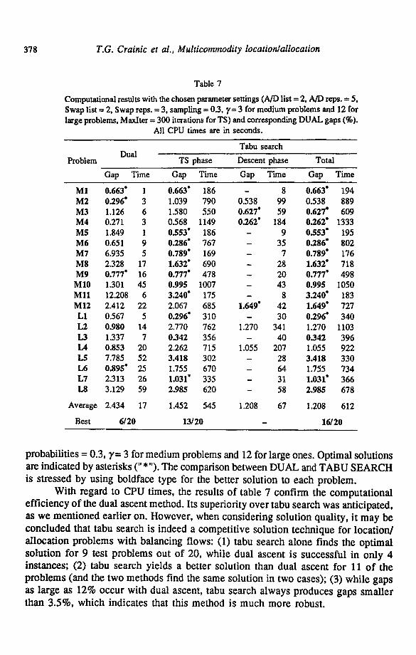
378 T.G. Crainic et al., Multicommodity location~allocation
Table 7
Computational results with the chosen parameter settings (A/D list = 2, A/D reps. = 5, Swap list = 2, Swap reps. = 3, sampling = 0.3, y= 3 for medium problems and 12 for large problems, MaxIter = 300 iterations for TS) and corresponding DUAL gaps (%).
All CPU times are in seconds.
Problem
Tabu search Dual
TS phase Descent phase Total
Gap Time Gap Time Gap Time Gap Time
M1 0.663" 1 0.663" 186 - 8 0.663" 194 M2 0.296" 3 1.039 790 0.538 99 0.538 889 M3 1.126 6 1.580 550 0.627* 59 0.627* 609 M4 0.271 3 0.568 1149 0.262" 184 0.262" 1333 M5 1.849 1 0.553" 186 - 9 0.553" 195 M6 0.651 9 0.286" 767 - 35 0.286" 802 M7 6.935 5 0.789" 169 - 7 0.789* 176 M8 2.328 17 1.632" 690 - 28 1.632" 718 M9 0.777" 16 0.777* 478 - 20 0.777* 498 M10 1.301 45 0.995 1007 - 43 0.995 1050 Ml l 12.208 6 3.240" 175 - 8 3.240* 183 M12 2.412 22 2.067 685 1.649" 42 1.649" 727 L1 0.567 5 0.296" 310 - 30 0.296" 340 L2 0.980 14 2.770 762 1.270 341 1.270 1103 L3 1.337 7 0342 356 - 40 0342 396 IA 0.853 20 2,262 715 1.055 207 1.055 922 I.,5 7.785 52 3.418 302 - 28 3.418 330 L6 0.895" 25 1.755 670 - 64 1.755 734 L7 2.313 26 1.031" 335 - 31 1,031" 366 L8 3.129 59 2,985 620 - 58 2.985 678
Average 2.434 17 1.452 545 1.208 67 1.208 612
Best 6/20 13/20 - 16/20
probabili t ies = 0.3, y = 3 for medium problems and 12 for large ones. Optimal solutions are indicated by asterisks C *"). The comparison between D U A L and T A B U S E A R C H is s tressed by using boldface type for the bet ter solut ion to each problem.
With regard to CPU times, the results o f table 7 conf i rm the computa t iona l e f f i c iency o f the dual ascent method. Its superior i ty o v e r tabu search was ant icipated, as we men t ioned ear l ier on. However , when cons ider ing so lu t ion qual i ty , i t m a y be
conc luded that tabu search is indeed a compet i t ive solut ion technique for loca t ion / a l loca t ion p rob lems with balancing flows: (1) tabu search a lone finds the op t imal so lu t ion for 9 test p roblems out o f 20, whi le dual ascent is successfu l in on ly 4 instances; (2) tabu search yields a be t te r solut ion than dual ascent fo r 11 o f the p rob lems (and the two me thods find the same solut ion in two cases); (3) whi le gaps as large as 12% occu r with dual ascent , tabu search a lways p roduces gaps smal le r than 3.5%, which indicates that this me thod is m u c h more robust.
T.G. Crainic et al., Multicommodity location/allocation 379
Furthermore, when a descent phase is appended to the tabu search procedure, improved solutions are found in 6 instances. The combined procedure obtains better solutions than DUAL for two more problems (a total of 14 out of 20) and 3 more optimal solutions for a total of 12 out of 20. Considering that on average the descent phase requires about 1/8 of the CPU time of the TS phase, it seems to be a worthwhile addition to the solution procedure.
5. Conc lus ions
We have presented a tabu search heuristic for solving location/allocation problems with balancing requirements. Extensive computational testing was performed on a set of benchmark problems. These tests showed that tabu search finds excellent, if not optimal, solutions to all problems in a reasonable amount of CPU time. Comparisons with a very effective dual procedure, especially customized for this class of problems, were quite favourable.
Since the proposed approach did not exploit the particular structure of the problem, it should be relatively easy to adapt it for solving similar problems complicated by additional constraints (e.g. budget constraints, capacity constraints, etc.). The results obtained are also very encouraging with regards to the perspectives of application of tabu search to mixed integer programming problems, in particular to those with an underlying network flow structure.
Appendix
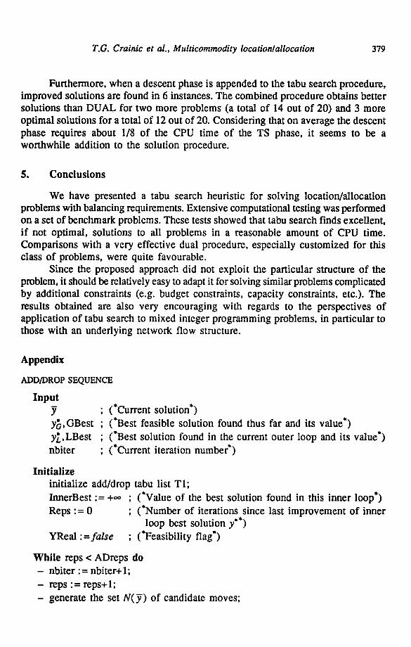
ADD~ROP SEQUENCE
Input y ; (*C~rrent solution*) yb,GBest ; (*Best feasible solution found thus far and its value*) y~,,LBest ; (*Best solution found in the current outer loop and its value*) nbiter ; (*Current iteration number*)
Init ial ize initialize add/drop tabu list T1; InnerBest := +0* ; (*Value of the best solution found in this inner loop*) Reps : = 0 ; (*Number of iterations since last improvement of inner
loop best solution y'*) YReal :=false ; (*Feasibility flag*)
While reps < ADreps do - nbiter : = nbiter+ 1; - reps : = reps+ 1; - generate the set N(y) of candidate moves;
380 T.G. Crainic et al., Multicommodity location/allocation
- select move s of N(y) having least esimated cost Z'(s(y)) and not in T1; - if every s in N(y) is tabu, select the one that has been in T1 the longest; - update T1, long-term memory and set y := s(y) ; - evaluate exact cost of new y, z ( y ) ; - if Z ( y ) < InnerBest t h e n
y ' : = y ;
InnerBest := Z(y) ; reps : = 0;
- if y is feasible then YReal := true; if Z ( y ) < LBest t h e n
Y~.:= y; LBest := Z(y) ;
if Z ( y ) < GBest then
yb := Y; GBest := Z(y) ;
e l s e
YReal :=false;
Output y°, InnerBest ; (*Best solution of inner loop so far and its value*) YReal ; (*Feasibility flag for y°*) y~., LBest ; (*Best solution and value obtained so far in this outer loop*) Yb, GBest ; (*Overall best feasible solution and value found so far*)
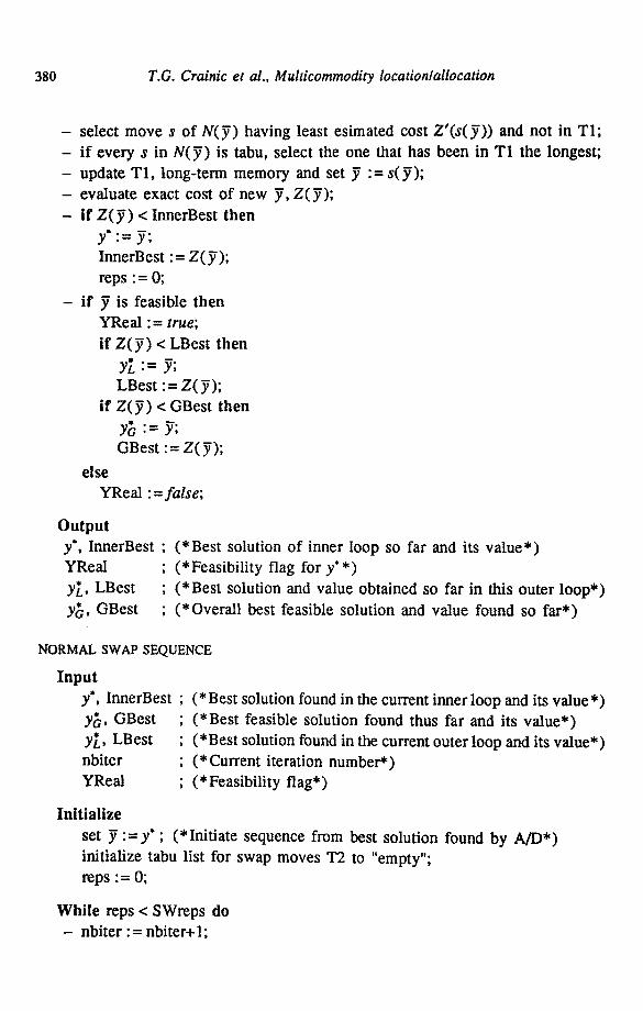
NORMAL SWAP SEQUENCE
I n p u t
y°, InnerBest ; (* Best solution found in the current inner loop and its value*) Yb, GBest ; (*Best feasible solution found thus far and its value*) y~., LBest ; (*Best solution found in the current outer loop and its value*) nbiter ; (*Current iteration number*) YReal ; (*Feasibility flag*)
I n i t i a l i z e
set y :=y'; (*Initiate sequence from best solution found by A/D*) initialize tabu list for swap moves T2 to "empty"; reps := 0;
W h i l e reps < SWreps d o
- nbiter : = nbiter+ 1;
T.G. Crainic et al., Multicommodity locationlaUocation 381
- reps := reps+l; - generate the set M(y) of candidate swap moves; - select move s of M(y-) having least estimated cost Z'(s(y)) and not in T2; - if every s in M(y-) is tabu, select the one that has been in T2 the longest; - update 'I"2, Ion-term memory and set y : = s( y-); - evaluate exact cost of new y, Z(y-); - if Z(y) < InnerBest then
y ' : = y;
InnerBest : = Z(y); reps : = 0;
- i f y is feasible then YReal := true; if Z(y) < LBest then
y; LBest : = Z(y-);
if z ( y ) < GBest then
yb := Y; GBest : = Z( y);
else YReal : =false;
O u t p u t
y' , InnerBest ; (*Best solution of inner loop so far and its value*) YReal ; (*Feasibility flag for y" *) y~,, LBest ; (*Best solution and value obtained so far in this outer loop*) yb, GBest ; (*Overall best feasible solution and value found so far*)
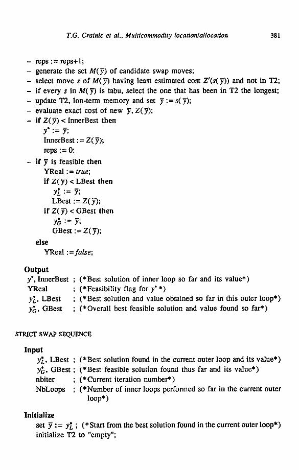
STRICT SWAP SEQUENCE
I n p u t
y~,, LBest ; (*Best solution found in the current outer loop and its value*) yb, GBest ; (*Best feasible solution found thus far and its value*) nbiter ; (*Current iteration number*) NbLoops ; (*Number of inner loops performed so far in the current outer
loop*)
I n i t i a l i z e
set y : = y~, ; (*Start from the best solution found in the current outer loop*) initialize T2 to "empty";
382 T.G. Crainic et al., Multicommodity location~allocation
reps : = 0; NbLoops : = NbLoops+ 1; Improve :=false; (*Flag indicating if LBest has been improved during this
sequence*)
While reps < SWreps do - nbiter := nbiter+l;
- reps : = reps+ 1; - generate the set M ( y ) of candidate swap moves; - select m o v e s of M ( y ) having least estimated cost Z'(s(y-)) and not in T2; - if every s in M(y-) is tabu, select the one that has been in T2 the longest;
- evaluate exact cost of ~ := s(y-), Z (~ ) ; - i f (Z(~) < LBest) and (Y feasible) t h e n
. =
LBest : = Z(~ ); Improve := true; reps : = 0; if Z ( ~ ) < GBest then
Yb : = 9 ; GBest : = Z(~) ;
e l s e
nbiter : = nbiter+ 1;
reps := reps+l;
set M(y-) := M(y)/{s}; return to the move selection step;
- i f improve = true then NbLoops := 0;
O u t p u t
YT., LBest yb, GBest NbLoops
; (*Best solution and value obtained so far in this outer loop*)
; (*Overall best feasible solution and value found so far*) ; (*Number of inner loops performed so far in this outer loop*)
A c k n o w l e d g e m e n t s
This work was partially funded by the Canadian Natural Sciences and Engineering Research Council and by the Fonds F.C.A.R. of the Province o f Quebec. This support is gratefully acknowledged. We also want to thank two anonymous referees for their valuable comments on an earlier version of this paper.

T.G. Crainic et al., Multicommodity locationlallocation 383
References
[1] A. Balakrishnan, T.L. Magnanfi and R.T. Wong, A dual-ascent procedure for large-scale uncapacitated network design, Oper. Res. 37(1989)716-740.
[2] T.G. Crainic, P.J. Dejax and L. Delorme, Models for multimode mulficoramodity location problems with interdepot balancing requirements, Ann Oper. Res. 18(1989)279-302.
[3] T.G. Crainic, L. Delorme and P.J. Dejax, A branch-and-bound method for multicommodity location with balancing requirements, Eur. J. Oper. Res. (1993), to appear.
[4] T.G. Crainic and L. Delorme, Dual-ascent procedures for multicommodity location/allocation problems with balancing requirements, Tramp. Sci. (1993), to appear.
[5] PJ. Dejax, T.G. Crainic and L. Delorme, Strategic/tactical planning of container land transportation systems, TIMS XXVIII/EURO IX Joins Meeting, Paris (1988).
[6] D. de Werra and A. Hertz, Tabu search techniques - A tutorial and application to neural networks, OR Spektrura 11(1989)131-141.
[7] M. Gendreau, A. Hertz and G. Laporte, A tabu search heuristic for the vehicle routing problem, Publication #777, Centre de Recherche sur les Transports, Universit6 de Montrtal (1991).
[8] F. Glover, Future paths for integer programming and links to artificial intelligence, Comput. Oper. Res. 13(1986)533-549.
[9] ' F. Glover, Tabu search, Part I, ORSA J. Comput. 1(1989)190-206. [10] F. Glover, Tabu search, Part H, ORSA J. Comput. 2(1990)4-32. [11] M.D. Grigoriadis and T. Hsu, RNET- The Rutgers minimum cost network flow subroutines, Rutgers
University, New Brunswick. New Jersey (1979). [12] Z.-Y. Guo, R~solution heuristique et optimale du probl~me de locallsation de d~lJtts avec ~.quilibrage,
Ph.D. Thesis, l~partement de Gtnie Industriel, Ecole Centrale, Paris (1990). [13] Z.-Y. Guo, T.G. Crainic and L. Delorme, Rtsolution heurestique du probl~me de localisation-
distribution avec 6quilibrage, Logistique/logistics: Production, distribution, transport/manufacturing, distribution" transportation, Proc. Conf. on the Practice and Theory of Operations Management and 4es jourr~es francophones sur la Logistique et les Transports, AFCET (1989) pp. 87-95.
[14] P. Hansen and B. Jaumard, Algorithms for the maximum satisfiability problem, Rutcor Research Report 93-87. Rutgers University (1987).
[15] J. Skorin-Kapov, Tabu search applied to the quadractic assignment problem, ORSA J. Comput. 2(1990)33-45.
[16] N. T~treauk, Une approche de restriction bas~e sur une m~thode primale-duale pour r~soudre le probl~me de Iocalisation-distribution avec (~changes int&d~ptts, M.Sc. Thesis, Publication #681, Centre de Recherche sur les Tranports, Unlversit~ de Montreal (1990).
[17] M. Widmer and A. Hertz, A new heuristic for solving the flow shop sequencing problem, Eur. J. Oper. Res. 41(1989)186-193.