a study of two investment strategies within swedish...

Strategic and tactical asset allocation - is it really used?

A study of two investment strategies within Swedish balanced funds

Johanna Gustafsson

Lund University

School of Economics and Management

The Department of Economics

Bachelor Thesis

Tutor: Erik Norrman

June, 2014

2

Abstract

Title: Stategic and tactical asset allocation - is it really used? - A study of two investment

strategies within Swedish balanced funds

Course: NekH01 – Bachelor thesis (15 credits)

Authour: Johanna Gustafsson

Advisor: Erik Norrman

Key words: Strategic asset allocation, tactical asset allocation, asset allocation, investment

strategies, balanced funds

Purpose: To examine if strategic and tactical asset allocation are used within Swedish balanced

funds and outline how these investment stratgies are used, by identifying trends.

Method: Compiled data over the asset allocation within swedish balanced funds 12 years back

will be analyzed by defining strategic and tactical asset allocation in quantitive terms. Hypothesis

tests will verify trends.

Conclusions: There are significant long term trends for three out of four asset classes. Over time,

the amount of equities has decreased and the amount of other derivatives and unit trusts have

increased. Tactical asset allocation has been used within Swedish balanced funds and it is a

function of stock index, conjunction indicator and interest rates for almost all asset types.

3

Table of Contents

1. BACKGROUND .................................................................................................................................. 5

1.1 Introduction ....................................................................................................................................... 5

1.2 Purpose and problem ........................................................................................................................ 6

1.3 Delimitation ........................................................................................................................................ 6

2. THEORY .............................................................................................................................................. 7

2.1 Modern portfolio theory ................................................................................................................... 7

2.2 Investment strategies ......................................................................................................................... 9

2.2.1 Asset Allocation .......................................................................................................................... 9

2.2.2 Strategic asset allocation .......................................................................................................... 10

2.2.3 Tactical asset allocation ........................................................................................................... 11

2.2.4 Applied modern portfolio theory ............................................................................................ 11

2.3 Econometric concepts ...................................................................................................................... 13

2.3.1 Regression analysis ................................................................................................................... 13

2.3.2 Hypothesis test .......................................................................................................................... 15

3. PREVIOUS RESEARCH ................................................................................................................. 17

4. METHODOLOGY ............................................................................................................................ 18

4.1 Scientific methods ............................................................................................................................ 19

4.2 Procedure ......................................................................................................................................... 21

4.3 Assumptions ..................................................................................................................................... 23

4.3.1 Defining strategic and tactical asset allocation ...................................................................... 23

4.3.2 Variables in regression analysis .............................................................................................. 24

4.3.3 Variables in hypothesis test ..................................................................................................... 25

4.4 Possible weakness in method .......................................................................................................... 27

5. DATA .................................................................................................................................................. 28

5.1 Primary data .................................................................................................................................... 28

5.2 Secondary data ................................................................................................................................ 30

6. RESULTS ........................................................................................................................................... 31

6.1 Hypothesis test – Strategic Asset Allocation ................................................................................. 31

6.1.1 Equities ...................................................................................................................................... 32

6.1.2 Bonds and Convertibles ........................................................................................................... 34

6.1.3 Other Derivatives...................................................................................................................... 36

6.1.4 Unit Trusts ................................................................................................................................ 38

4

6.2 Hypothesis test – Tactical Asset Allocation ................................................................................... 40

6.2.1 Equities ...................................................................................................................................... 40

6.2.2 Bonds and Convertibles ........................................................................................................... 41

6.2.3 Other Derivatives...................................................................................................................... 43

6.2.4 Unit Trusts ................................................................................................................................ 44

6.3 Summary of results ......................................................................................................................... 45

7. ANALYSIS ......................................................................................................................................... 46

8. CONCLUSION .................................................................................................................................. 48

9. FURTHER RESEARCH .................................................................................................................. 48

10. BIBLIOGRAPHY .............................................................................................................................. 49

10.1 Books .............................................................................................................................................. 49

10.2 Journal articles .............................................................................................................................. 50

10.3 Electronic sources .......................................................................................................................... 51

11. APPENDIX ......................................................................................................................................... 53

11.1 Regression analysis – strategic asset allocation .......................................................................... 53

11.1.1 Equities .................................................................................................................................... 53

11.1.2 Bonds and Convertibles ......................................................................................................... 54

11.1.3 Other derivatives .................................................................................................................... 55

11.1.4 Unit trusts ................................................................................................................................ 56

11.2 Regression analysis – tactical asset allocation ............................................................................. 57

11.2.1 Equities .................................................................................................................................... 57

11.2.2 Bonds and Convertibles ......................................................................................................... 57

11.2.3 Other derivatives .................................................................................................................... 58

11.2.4 Unit trusts ................................................................................................................................ 59

5

1. BACKGROUND

This chapter will serve as an introduction. It will present the problem and the purpose of this

thesis. It will also outline relevant delimitations.

1.1 Introduction

If modern portfolio theory would be applicable on all markets and all asset and investors would

believe in CAPM (Capital Asset Pricing Model), the best alternative would then be to invest in

the market portfolio, an index fund.1

Fortunately for the fund industry, people believe that individual fund managers can outperform

the market. Otherwise there would not be 30 billion Swedish kronor in hedge funds, during the

beginning of 2014.2 As a hedge-fund manager, or a fund manager for any fund that is not an

index fund, you are expected to beat the performance of passive investments even after risk has

been considered.3 This is where investment strategies comes in. The purpose with an investment

strategy is to maximize the wealth of an investment over a period of time. An investment strategy

could be anything from investing according to patterns of historical prices or looking for

arbitrage.4 In simple terms, it could be security selection or asset allocation.5

This thesis will analyze the usage of asset allocation within Swedish balanced funds. It will

examine strategic asset allocation (long term) and tactical asset allocation (short term). It will also

present a definition and relevant terms in order to understand investment strategies. Hence, a

quote by Meir Statman will initially introduce the differences in an illustrative way;

“Good strategic asset allocation is like tailoring a well-fitting suit. Good tactical asset allocation and

security selection is weaving the suits fabric at a low cost. Both are important, but they are distinct. High-

quality fabric woven at a low cost provides little comfort when it drapes a size 40 body in a size 46 suit.”6

1 H Byström, Finance – Markets, Instruments and Investments, Studentlitteratur, Lund, 2007, p. 15 2 Nysparande och fondförmögenhet 2014, http://www.fondbolagen.se/Statistik--index/Nysparande-i-fonder/ 2014-

04-19 3 H Byström, Finance – Markets, Instruments and Investments, p. 15 4 C Erlwein, R Mamon, M Davidson, ‘An examination of HHM-based investment strategies for asset allocation’,

Applied Stochastic Models in Business and Industry, December 2009, pp. 1 5 Z Bodie, A Kane, A Marcus, Investments and Portfolio Management, ninth edition, McGraw Hill, New York,

2011, p. 36 6 M Statman, The 96,3 % Question of Financial Advisors, 2000, pp. 16

http://www.fondbolagen.se/Statistik--index/Nysparande-i-fonder/

6

1.2 Purpose and problem

The purpose of this text is to examine strategic and tactical asset allocation and see whether and

how the investment strategies are used in a practice. The aim is to identify general trends, upon

which the conclusion will rely on. The research will be done quantitatively on Swedish balanced

funds with support of relevant literature. A multiple regression analysis and hypothesis testing

will be done in order to quantify the results. The problem that the thesis will answer follows:

Are strategic and tactical asset allocation used within Swedish balanced funds in a way that

trends could be identified?

The two different investment strategies will be quantified and compared in relation to stock

market, conjunction indicator and interest rate.

1.3 Delimitation

In order to write this thesis according to the given guidelines, some delimitation will be

determined.

To start with the data is delimit to Sweden, and fund companies that are under the Financial

Supervisory Authority, Finansinspektionen. I consider my knowledge of the Swedish market

superior to my knowledge within other markets, and the data for Swedish funds easier to access.

The second delimitation is by only researching on balanced funds. For the definition of balanced

funds, this thesis refers to a definition by Morningstar:

“A mutual fund that has an investment mandate of "balancing" its portfolio holdings. The fund generally

includes a mix of stocks and bonds in varying proportions according to the fund's investment outlook.”7

These funds are considered to more flexible than other funds in the asset allocation between asset

classes.

7 Morningstar: Balanced Fund, http://www.morningstar.com/InvGlossary/balanced_fund_definition_what_is.aspx

2014-02-06

http://www.morningstar.com/InvGlossary/balanced_fund_definition_what_is.aspx

7

2. THEORY

Relevant theories will be presented in this chapter; a brief presentation of modern portfolio

theory and explanations regarding the concepts of investment strategies, asset allocation,

strategic asset allocation as well as tactical asset allocation. An outline of regression analysis

and hypothesis testing will also be included for readers not familiar with these concepts.

2.1 Modern portfolio theory

Modern portfolio theory is often considered founded by Harry Markowitz in 1952 and the

development of the mean-variance analysis. According to this analysis, there is a best way of

maximizing return (mean) given a preferred level of risk (variance), for investors who cares only

about return and risk. In the diagram below stocks are representing assets with high risk and

bonds are representing assets with low risk. 8 There are numerous of kinds of other assets that

could be included in a portfolio, but these will not be considered in order to simplify the model.

The curved line in the diagram below is called the portfolio frontier, it illustrates possible

combinations of assets with higher risk and assets with lower risk. The investor should choose a

combination that will put them as much to the up-left on the curve as possible. The upper part of

the curve is called the efficient frontier, all portfolios on the upper part of the curve will have the

same risk but higher expected return than portfolios on the lower part of the curve.9

A straight line illustrate the set of means and standard deviations that could be achieved when

cash is added to a portfolio on the curved line. The point where the two lines touch is called the

tangency portfolio, which is the best mix of stocks and bonds. According to financial theory,

every investor who cares about only mean and variance should hold the tangency portfolio but

add more or less cash, depending on their risk-preferences.10

8 J Campbell, , LM Viceira, Strategic Asset Allocation: Portfolio Choice for Long Term Investors, Oxford University

Press: 2002, p. 2 9 H Byström, Finance – Markets, Instruments and Investments, p. 131-134 10 J Campbell, , LM Viceira, Strategic Asset Allocation: Portfolio Choice for Long Term Investors, pp. 2

8

Figure 1. Mean-Variance Diagram11

The mean-variance analysis has been developed into CAPM, Capital Asset Pricing Model, an

equilibrium theory of the market portfolio. The model is stating that all asset in the long term will

be a part of the market portfolio and therefore be paid the price of their risk premium, an

equilibrium price. Attempts to outperform the market portfolio will consequently be unnecessary,

since all asset is priced correctly.12

11 Ibid., pp. 3 12 Z Bodie, A Kane, A Marcus, Investments and Portfolio Management, p. 308-311

9

2.2 Investment strategies

The purpose with investment strategies is to maximize the wealth of an investment over a period

of time. The mean-variance model, accounted for in previous chapter, is a classical model aiming

to maximize return in relation to risk. An essential factor of the model is the adoption of an

efficient market. Investors who do not believe that the market is efficient, will instead use

investment strategies in order to benefit from the inefficiencies. Technical analysis of historical

asset prices and arbitrage strategies are two examples of such investment strategies.13

Essentially, there are two types of investment decisions within investment strategies. Asset

allocation is the decision between broad asset classes, and security selection is the decision of

particular securities.14 This chapter will only focus on asset allocation, since security selection is

less relevant for this thesis.

2.2.1 Asset Allocation

Asset allocation as an investment strategy aims to allocate the investments among different types

of assets in order to match the investors risk tolerance, goals and time horizon. A general

consensus within finance is that there are no such thing as a general asset allocation, it is rather an

investment strategy starting from individual preferences as illustrated in mean-variance diagram

above. Although, asset allocation focus on the asset classes rather than individual securities.15

There is no definite definition of what an asset class is even though asset allocation is a widely

known concept. Asset allocation could be defined in comprehensive terms, including only three

different asset types – equities, bond and cash. By defining asset allocation in a comprehensive

way there is a risk that there are securities who could not be clearly defined, such as derivatives.

13 C Erlwein, R Mamon, M Davidson, ‘An examination of HHM-based investment strategies for asset allocation’,

Applied Stochastic Models in Business and Industry, p. 1 14 P Z Bodie, A Kane, A Marcus, Investments and Portfolio Management, p. 36 15 Investopedia: Asset Allocation, http://www.investopedia.com/terms/a/assetallocation.asp#ixzz1QTuSzfhn 2014-

03-31

http://www.investopedia.com/terms/a/assetallocation.asp#ixzz1QTuSzfhn

10

An alternative approach of defining is according to cash flow; capital assets,

consumable/transformable assets and store-of value assets. According to this definition stocks

and bonds would be categorized as capital assets, commodities as consumable/transformable

assets and fine-art as store-of-value assets.16

2.2.2 Strategic asset allocation

Strategic asset allocation is a buy and hold strategy with target allocations for different asset

classes. The target allocation depends on different factors, such as the time horizon, risk-

willingness and the type of assets that investments are allocated between. If the investor’s

references change over time, the target allocation will consequently have to change. The portfolio

will also have to be rebalanced back to the original strategic target allocations, if the performance

of the different assets classes change the original proportions.17

The term strategic asset allocation was coined by Brennan, Schwarz and Lagnado, in 1997 in the

paper “Strategic Asset Allocation”, described as a long-term response to time-varying investment

opportunities.18

The optimal portfolio on the efficient frontier, in Markowitz mean-variance model, have been

seen as a static, one-period, strategic asset allocation decision. Although, financial actors such as

pension funds, usually have a planning horizon many years ahead and cannot for that reason use a

static, one-period asset allocation decision. Strategic asset allocation in practice is more

dynamic.19

16 T Idzorek, Strategic Asset Allocation and Commodities, Ibbotson, Chicago, 2006, pp. 3-4 17 Investopedia: strategic asset allocation http://www.investopedia.com/terms/s/strategicassetallocation.asp 2014-03-

31 18 J Campbell, YL Chan, M Viceira, ‘A multivariate model of strategic asset allocation’, Journal of Financial

Economics’, vol. 67, January 2002, pp. 42 19 TK Sui, ‘Long-term strategic asset allocation with inflation risk and regime switching’, Quantitative Finance, vol.

11, May 2009, pp. 1

http://www.investopedia.com/terms/s/strategicassetallocation.asp

11

2.2.3 Tactical asset allocation

One of the earliest to introduce tactical asset allocation was Harry Markowitz, describing it as a

“systematic allocation of investment portfolios across broad asset classes such as bonds, stocks

and cash”. As an investment strategy, tactical asset allocation gained popularity with the crash of

the stock market in 1987. By investing according to the strategy investors would have been able

to avoid being affected of the crash, by allocating their money from equities to other assets in

time.

Tactical asset allocation is a matter of timing, it is a single period strategy which requires the

investor to have a mean-variance criteria defined over one period. According to Brennan,

Schwarz and Lagnado, there are two critical aspects with tactical asset allocation. First, returns

are often not defined in a single period and by having such a short-term strategy, one have to

make a proxy. Secondly, since the timing in tactical asset allocation is crucial the investor must

be able to predict the future market returns in a correct way. An investor which invests according

to the tactical asset allocation strategy cannot believe in the random walk hypothesis.2021

2.2.4 Applied modern portfolio theory

The theory of the efficient frontier is applicable on investment strategies such as strategic and

tactical asset allocation. The diagram below shows the efficient frontier, which is only the upper

part of the portfolio frontier curve. As mentioned in previous chapter, all portfolios on the upper

part of the curve will have the same risk but higher expected return than portfolios on the lower

part of the curve.22

Tactical asset allocation could be described as a shift of the efficient frontier. It is illustrated in

the diagram below as a shift from 1 to 2. Strategic asset allocation, on the other hand, is a shift on

20 M Brennan, ES Schwarz, R Lagnado, ‘Strategic Asset Allocation’, Journal of Economic Dynamics & Control, vol.

21, 1997, pp. 1377-1378 21 Definition: “The theory that stock price changes have the same distribution and are independent of each other, so

the past movement or trend of a stock price or market cannot be used to predict its future movement.”

http://www.investopedia.com/terms/r/randomwalktheory.asp 2014-03-31 22 H Byström, Finance – Markets, Instruments and Investments, p. 131-134

http://www.investopedia.com/terms/r/randomwalktheory.asp

12

the efficient frontier. It is illustrated as a shift from A to B in the figure below. Strategic asset

allocation requires a selection of assets that fits the risk attitudes of the investors, and it could be

described as the management of investors. Tactical asset allocation could then be described as the

management of investments.23

Figure 2. Strategic Asset allocation versus Tactical Asset allocation24

23 M Statman, The 96,3 % Question of Financial Advisors, pp. 17 24 Ibid., pp. 17

13

2.3 Econometric concepts

2.3.1 Regression analysis

A regression analysis is used in order to analyze a relationship between two variables, where both

variables are quantitative and assume many values. In order to analyze a relationship between

more than two variables, a multiple regression analysis is used.25 Below is presented an example

of a summary output on a multiple regression analysis. This example is taken from a multiple

regression analysis done in this essay, where the relationship between equities and stock index,

purchasing manager index and interest rates index is analyzed. A simple regression analysis will

not be presented since it is done in the same way but with only one variable.

Figure 3. Regression Analysis

There are two types of variables in a regression analysis, the X-variables, also known as the

independent variables (in this example OMX Stockholm 30 index, Swedbank PMI and

25K Dahlström, Från datainsamling till rapport, femte upplagan, Studentlitteratur, 2001, p. 218

SUMMARY OUTPUT

Regression Statistics

Multiple R 0.6052

R Square 0.3663

Adjusted R Square 0.3176

Standard Error 1.7170

Observations 43.0000

ANOVA

df SS MS F Significance F

Regression 3.0000 66.4665 22.1555 7.5148 0.0004

Residual 39.0000 114.9816 2.9482

Total 42.0000 181.4481

Coefficients Standard Errort Stat P-value Lower 95%Upper 95%Lower 95.0%Upper 95.0%

Intercept 96.2039 2.2239 43.2590 0.0000 91.7056 100.7021 91.7056 100.7021

OMX Stockholm 30 index -0.0038 0.0102 -0.3753 0.7094 -0.0244 0.0168 -0.0244 0.0168

Swedbank PMI 0.0096 0.0230 0.4166 0.6793 -0.0369 0.0560 -0.0369 0.0560

Stockholm Interbank Rate 3M 0.0397 0.0088 4.4999 0.0001 0.0219 0.0576 0.0219 0.0576

14

Stockholm Interbank Rate 3M) and the Y-variable, also known as the examined variable or the

dependent variable (in this example equity).26

When plotting these variables in a graph, a relationship could (or could not) be identified by a

regression line. A least square method is then used to calculate regression coefficients in order to

make the squared distance between the actual plot and the estimated regression line as small as

possible.27 The formula of regression line is determined as:

�̂� = 𝑏0 + 𝑏1𝑋1 + 𝑏2𝑋2 + 𝑏3𝑋3

The coefficient in front of X1 is recognized as the average change in Y if X1 increase one unit and

all other independent variables are fixed.28 The regression line of the above example would then

be:

�̂� = 𝑏0 − 0.0038𝑋𝑂𝑀𝑋𝑆 + 0.0096𝑋𝑃𝑀𝐼 + 0.0397𝑋𝑅𝑎𝑡𝑒 3𝑀

From this line a conclusion could be drawn; if OMXS is increased by one unit, the amount of

equity is lowered by 0.0038 units.

The standard error next to the coefficient is the standard error of the slope coefficient.29 It is

recognized as the distance of the regression line from the points of the independent variables.30

The t-statistics is defined as

𝒕𝒃𝟏 =𝒃𝟏 − 𝜷𝟏

𝒔𝒃𝟏

In most regression programs, such as the one in Microsoft Excel, β1 is defined as zero.

𝜷𝟏 = 𝟎

Student’s t-statistics will therefore be the coefficient divided by the standard error.31

26 Ibid., p. 219 27 Ibid., p. 221-222 28 Ibid., p. 224 29 P Newbold, WL Carlson, BM Thorne, Statistics for Business and Economics, eight edition, Pearson, USA, 2013,

p. 441 30 Ibid., p. 439 31 Ibid., p. 440

15

𝒕𝒃𝟏 =𝒃𝟏− 𝜷𝟏

𝒔𝒃𝟏 =

𝒃𝟏

𝒔𝒃𝟏

R2 is the squared correlation coefficient, it is the coefficient of determination and could be

explained as the percent explained variability. With some exemptions, the higher values indicated

better regression.32

2.3.2 Hypothesis test

A hypothesis test is a way of testing a causation, often an experiment including a number of units

such as persons, mice or municipals.33 In this thesis the units will be different asset classes. A

common example of a hypothesis test is testing the effect of new pharmaceuticals. A number of

people (or animals) is then divided in two groups, where one group is treated with the

pharmaceutical and the other with placebo. If the difference between the two groups are so

considerable that it could not have been caused randomly, the difference is then said to be

significant.34

When testing a hypothesis on a regression analysis the aim is to determine if there is a

relationship or not. If the regression slope is determined by β1 and β1 equals 0 a conclusion could

be done that there is no relationship or trend between the independent and the dependent variable,

X and Y. The hypothesis will then be denoted:

𝑯𝟎: 𝜷𝟏 = 𝟎

𝑯𝟏: 𝜷𝟏 ≠ 𝟎35

32 Ibid., p. 435 33 K Dahlström, Från datainsamling till rapport, p. 382 34 Ibid. 35 P Newbold, WL Carlson, BM Thorne, Statistics for Business and Economics, p. 440

16

H0 is the null hypothesis and H1 is the alternative, which is valid if the null hypothesis is

rejected.36 In a hypothesis test of a regression analysis a test variable is used to test the null

hypothesis. There are different methods for testing a hypothesis, and below will only be

presented the method that is relevant for this thesis. Given that b1 is normally distributed, this will

be denoted:

𝒕𝒃𝟏 =𝒃𝟏 − 𝜷𝟏

𝒔𝒃𝟏

Since the null hypothesis is β1 equals 0 (there is no relationship) this could be rewritten as

𝒕𝒃𝟏 =𝒃𝟏

𝒔𝒃𝟏

If b1 is the coefficient of the independent variable and sb1 is the standard deviation of this

coefficient then Student´s t-statistics will be the division of these. If the t-statics is a large number

a conclusion could be drawn that there is a strong evidence to reject the null hypothesis and a

strong relationship between the dependent and the independent variable. In order to determine a

limit of an acceptable t-statistics a decision rule is set before the test.

H0 is rejected if

𝒃𝟏 − 𝜷𝟏

𝒔𝒃𝟏> 𝒕𝒏−𝑲−𝟏,𝜶/𝟐

or

𝒃𝟏 − 𝜷𝟏

𝒔𝒃𝟏< −𝒕𝒏−𝑲−𝟏,𝜶/𝟐

37

36 K Dahlström, Från datainsamling till rapport, p. 241 37 P Newbold, WL Carlson, BM Thorne, Statistics for Business and Economics, p. 442, 497

17

𝒕𝒏−𝑲−𝟏,𝜶/𝟐 is the critical value, a number gained from a table. It consists of the number of

observations, the number of categories and the confidence interval.38 A 95% confidence interval

means that 95% of all intervals will cover the true value with a normally disturbed curve.39 Alfa

is the number 1 subtracted by the confidence interval, for example 5%. In a two-tailed test with

60 observations and a 95% confidence interval, a Student´s t-statics with a greater value than 2

indicate that there is a relationship between the dependent and the independent variable.40

A confirmation could be done by looking at the p-value, because the p-value is the probability

that the null hypothesis is true.41

3. PREVIOUS RESEARCH

This chapter serve as an overview to relevant previous research about strategic and tactical

asset allocation.

In 1986, Gary Brinson, L. Randolph Hood and Gilbert Beebower published a six page article on

the topic “Determinants of Portfolio Performance”. In the article, they concluded that 96, 3% of

the variation in total pension plan returns could be explained by investment policy. To Brinson

and Hood, the article was a way to establish a theory they have come up with when working with

institutional pension clients. They argued that there was too much focus on the selection of

investment managers and too little focus on reviewing asset allocation policies. The research was

done 1974 -1983 on 91 large corporate pension plans. In brief, it concluded that the proportions

of broad asset classes included in the portfolio had a significant effect of the return.42 The article

started a debate on asset allocation and portfolio performance43.

38 P Newbold, WL Carlson, BM Thorne, Statistics for Business and Economics, p. 440-443 39 K Dahlström, Från datainsamling till rapport, p. 273 40 P Newbold, WL Carlson, BM Thorne, Statistics for Business and Economics, p. 440-443 41 P Newbold, WL Carlson, BM Thorne, Statistics for Business and Economics, p. 441 42 RL Hood, ‘Determinants of Portfolio Performance - 20 years later’, Financial Analysts Journal, 2005, pp. 6 – 7 43 Ibid., pp. 8

18

One of the debaters was William Jahnke, whom in 1997 published “The Asset Allocation Hoax”

in which he strongly criticized the article in several ways. As an example, he argued that asset

weights for an investor should not fixed as they were in the research. The expected return, he

said, could not be fixed, since the investment opportunities differs over time.44

In 2000, Meir Statman discussed both views in “The 96, 3% Question of Financial Advisors”. He

concluded that Brinson, Hood and Beebower were correct when arguing that strategic asset

allocation was more important than tactical asset allocation and security selection. But, in

contrary to their findings, he concluded that it was because of the 1, 1% detracted from the return

by using tactical asset allocation and security selection. He argued that financial advisors should

focus on investor management rather than investment management.45

Roger G. Ibbotson and Paul D. Kaplan published in 2000 a research on whether asset allocation

explains 40, 90 or 100 percent of the performance. They concluded that it was a matter of the

way asking the question. Focusing on the variation of the return among funds that are explained

by policy, it is 40 percent. But in a typical fund and the variability in return across time, 90

percent is explained by policy. Finally, on average 100 percent of the level of returns is explained

by the policy return level.46

4. METHODOLOGY

In the chapter of methodology the scientific methods for this essay will be presented. The

procedure of the examination will be described as well as definitions of concepts. In addition

to this, an outline will be presented of the statistical methods used in the regression analysis

and hypothesis testing. In the end of this chapter, possible weaknesses will be accounted for.

44 W Jahnke, ‘The Asset Allocation Hoax’, Financial Design – White paper, vol. 1, February 1997, pp. 3 45 M Statman, Meir, The 96,3 % Question of Financial Advisors, pp. 19 46 RG Ibbotson, PD Kaplan, Does Asset Allocation Policy Explain 40,90 or 100 percent of Performance, Financial

Analysts Journal, Jan/Feb 2000, pp. 26

19

4.1 Scientific methods

There are three research philosophies to consider; positive, hermeneutic and critical. A strict

positive philosophy will rely on a quantitative method and logical reasoning. With this approach,

a thesis will serve as an observation. A positive research philosophy have been used throughout

this thesis.

A hermeneutic philosophy is stating the opposite, and a thesis with a hermeneutic approach will

be an interpretation rather than an observation. Critical research philosophy is a mix of the

positive and hermeneutic, aiming to combine the participating and observing perspective.47

Figure 4. Research philosophy

A thesis also could be either quantitative or qualitative. A quantitative method is used when the

primary data is based on a numerical observation or can be transformed into a numerical

observation. 48 A qualitative method is on the contrary not a numerical observation, the

observation or conclusion is often instead examined by using words as a tool.49 Quantitative data

is normally regarded as “hard facts” and qualitative data as “soft facts”. 50

47 F Wiederheim-Paul, LT Eriksson, Att utreda, forska och rapportera, Liber ekonomi, Malmö, 1999 p. 218-222 48 J Backamn, Rapporter och Uppsatser, Studentlitteratur AB, Lund, 2010, p. 33 49 Ibid., p. 33 50 F Wiederheim-Paul, LT Eriksson, Att utreda, forska och rapportera, p. 65

RESEARCH APPROACH

DEDUCTIVE INDUCTIVE

METHOLOGICAL APPROACH

QUANTIATIVE QUALITATIVE

RESEARCH PHILOSOPHY

POSITIVE HERMANUETIC CRITICAL

20

For this thesis, a quantitative method was selected. A qualitative method could have been done by

interviews. A quantitative method was considered to be superior because it provided a more

general view that contained more information than a qualitative would have given.

Figure 5. Methodological approach

Finally, there are two types of logical reasoning; deductive reasoning and inductive reasoning.

The approach the author choose to take affects the pattern to which the final conclusion is

reached.51

Deducative reasoning is normally the easiest form of logical reasoning. A deductive reasoning

consist of major and minor arguments that are linked together. A conclusion is drawn by simply

putting them together. For instance; a first argument “birds fly”, and a second argument “I am a

bird”. The conclusion with deductive reasoning will be: “therefore I fly”.52 A deductive reasoning

has been used in this thesis due to the quantitative material that have been available.

Inductive reasoning is more complex since it implicates an identification of common factors

among arguments that are not necessary linked to each other.53 An example with using inductive

reasoning could be; “She studies diligent”, “She has intelligent parents”, “She masters social

51B Minto, The pyramid principle. Logic in writing and thinking, third edition, Pearson Education, Essex, 2009, p. 63 52 Ibid., p. 63-67 53 Ibid.,, p. 69

RESEARCH APPROACH

DEDUCTIVE INDUCTIVE



RESEARCH PHILOSOPHY


21

skills”. From those three arguments the conclusion will then be: “She has keys to success in

today’s society”.54

Figure 6. Research approach

4.2 Procedure

To collect information about all Swedish balanced funds and their holdings, information was

gained from the website of the Swedish Financial Supervisory Authority, Finansinpektionen.55

As a government authority they are collecting information from all fund companies under their

supervision, and it is a requirement for almost every financial services company to be under their

supervision.56 The information from the fund companies regarding their holdings is compiled

quarterly and regards the last business day the previous quarter.57

54 SÅ Hörte, Hur kan man ge struktur åt rapporter och uppsatser?, Luleå Tekniska Universitet, Avdelningen för

Industriell Organisation, pp. 7 55 Swedish Financial Supervisory Authority – Fund holdings, http://fi.se/Register/Fondinnehav/ 2014-03-31 56 Swedish Financial Supervisory Authority – Registered companies not under the supervisory of FI,

http://fi.se/Register/Foretagsregistret/Registrerade-foretag-som-inte-star-under-FIs-tillsyn/ 2014-03-31 57 Swedish Financial Supervisory Authority – About fund holdings, http://fi.se/Register/Fondinnehav/Om-

fondinnehav/ 2014-03-31

RESEARCH APPROACH

DEDUCTIVE INDUCTIVE



RESEARCH PHILOSOPHY


http://fi.se/Register/Fondinnehav/

http://fi.se/Register/Foretagsregistret/Registrerade-foretag-som-inte-star-under-FIs-tillsyn/

http://fi.se/Register/Fondinnehav/Om-fondinnehav/


22

To identify balanced funds in the information from the Swedish Financial Supervisory Authority

a categorization was used from the Swedish version of Morningstar. Morningstar categorize

funds based on the previous three years portfolio statistics. New funds are categorized based on

an estimate and thereafter given a more permanent category when portfolio statistics is

available.58

I wanted to specifically look at balanced funds since my view was that they normally have the

possibility to allocate with less restrictions than e.g. equity funds.

After identifying all the balanced funds, the relevant information was collected of which funds to

include and their holdings. Although the holdings were specified, such as “H&M B”, there was a

need to identify the asset class for this instrument as the correct one, in this case “equities”. In

order to do so, ISIN was used. ISIN is the “International Securities Identification Number”, it is a

worldwide system to classify securities. Every security has a 12 digit ISIN-number, which consist

of a mixture of letters and numbers.59

The program Datastream was then used to identify what kind of asset class every ISIN-number

was connected to. Some of the holdings were not able to be identified by their ISIN in

Datastream or by other resources. In those cases they had to be manually categorized by their

name. By identifying common identifiers, such as Ltd, Fut, AK all holdings that were not

categorized by Datastream could be identified. This created a complete workbook telling which

balanced funds with what asset type that had existed the last twelve years.

The data was tested in a simple and multiple regression analysis based on set definitions. OMX

Stockholm 30 Index, Swedbank PMI SA and Stockholm interbank rate 3 months was collected

from Bloomberg in order to identify trends. Hypothesis tests evaluated the significance of the

initially asked problem.

58 Morningstar – Category, http://www.morningstar.com/InvGlossary/morningstar_category.aspx 2014-03-31 59 ISIN, http://www.isin.org/isin/ 2014-03-31

http://www.morningstar.com/InvGlossary/morningstar_category.aspx

http://www.isin.org/isin/

23

4.3 Assumptions

4.3.1 Defining strategic and tactical asset allocation

In order to gain information about strategic and tactical asset allocation the allocations had to be

defined in relation to the data. When doing so, the long term trend was determined to be define as

strategic asset allocation, and the deviation from that line as the tactical asset allocation. Below is

an example illustrating strategic and tactical asset allocation, the dotted line marks the strategic

asset allocation and the filled line marks the tactical asset allocation.

Figure 7. Illustration of strategic and tactical asset allocation

0.00%

0.50%

1.00%

1.50%

2.00%

2.50%

3.00%

3.50%

Asset Class

Tactical Asset Allocation Strategic Asset Allocation

24

The reason for defining strategic asset allocation as a long term trend and not as a fixed average

was because the information gained from an average would not be as accurate as the trend. As

argued by Meir Statman;

“..but investors might change their strategic asset allocations if they change their trade-off

between their expected returns and risk. Investors might also change their strategic asset

allocations if they revise their estimates of expected returns or risk, but strategic asset allocation

are found on the acceptance of the current market valuations, not on challenge to them.”

If strategic asset allocation had been fixed, changes in long term investment policies or closed

and open balanced funds would not have been taken into consideration. For that reason, strategic

asset allocation was chosen to be defined as the long term trend of tactical asset allocation and

not as a fixed average.

Further explained by Meir Statman the tactical asset allocation is a way of timing the market and

doing shifts in asset allocations.60 The conclusion was made that this would best be interpreted

from the deviations from what was defined as the strategic asset allocation.

4.3.2 Variables in regression analysis

The regression used for the strategic asset allocation only tested one independent variable, time.

The dates were indexed from 1-46 with a gap for the three quarters were the Financial

Supervisory Authority did not have the information. It was 43 observations in total.

The regression used for the tactical asset allocation was consisting of three variables other than

the dependent variable, Y.

�̂� = 𝑏0 + 𝑏1𝑋𝑂𝑀𝑋𝑆 + 𝑏2𝑋𝑃𝑀𝐼 + 𝑏3𝑋𝑅𝑎𝑡𝑒 3𝑀

XOMX is the OMX Stockholm 30 Index. The index consist of the 30 most traded stocks at

OMXS.61 It was compared to Stockholm all share, but due to higher volatility the OMX

60 M Statman, The 96,3 % Question of Financial Advisors, pp. 2 61 Avanza – OMXS30, https://www.avanza.se/index/om-indexet.html/19002/omx-stockholm-30, 2014-04-19

https://www.avanza.se/index/om-indexet.html/19002/omx-stockholm-30

25

Stockholm 30 Index was considered more useful for the analysis, since the market trends were

more significant.

XPMI is the Swedbank PMI Index. It is a purchasing manager index that consist of 200 purchasing

managers within manufacturing in Sweden. It is a conjunction indicator founded in 1994.62 A

GDP measurement would have been an alternative way of approaching the behavioral finance

through an indicator. Although, Swedbank PMI was considered giving more up-to date indicator

of the market view.

XRate 3M is the Stockholm interbank rate, Stibor, 3 months. It is a reference rate showing an

average of interest rates that are being offered amongst a number of Swedish banks called

Stiborbanks. The 3 months rate is the average rate without collaterals.63 Repo rate was considered

as an alternative to Stibor, but Stibor was considered favorable due to stronger reflections of

economic conditions and market view. Other lengths of the Stibor rate could also have been used,

but 3 months was considered relevant due to the horizon of tactical asset allocation.

The variables included three different aspects that affects the asset allocation; stock market,

conjunction indicator and interest rate. There are many parameters left out, which is a possible

weakness, but these three variables were considered the most relevant.

4.3.3 Variables in hypothesis test

The hypothesis test was done according to theoretical methods, presented in Chapter 2.3.2

Hypothesis test. The following variables were included:

Hypothesis

𝑯𝟎: 𝜷𝟏 = 𝟎

𝑯𝟏: 𝜷𝟏 ≠ 𝟎

62 Swedbank – PMI, http://www.swedbank.se/om-

swedbank/analyser/samhallsekonomi/inkopschefsindex/inkopschefsindex,-mal-och-metodik/index.htm, 2014-04-19 63 National bank of Sweden – Explanation of the series, http://www.riksbank.se/sv/Rantor-och-

valutakurser/Forklaring-till-serierna/Svenska-marknadsrantor/, 2014-04-19

http://www.swedbank.se/om-swedbank/analyser/samhallsekonomi/inkopschefsindex/inkopschefsindex,-mal-och-metodik/index.htm


http://www.riksbank.se/sv/Rantor-och-valutakurser/Forklaring-till-serierna/Svenska-marknadsrantor/


26

Test variable

𝒕𝒃𝟏 =𝒃𝟏 − 𝜷𝟏

𝒔𝒃𝟏

Decision rule,

H0 rejected if

𝒃𝟏 − 𝜷𝟏

𝒔𝒃𝟏> 𝒕𝒏−𝑲−𝟏,𝜶/𝟐

or

𝒃𝟏 − 𝜷𝟏

𝒔𝒃𝟏< −𝒕𝒏−𝑲−𝟏,𝜶/𝟐

64

The variance of the population was unknown, therefore a student´s t-statistics was used.65 The

level of significance, α, was set to 5% and hence a confidence interval was determined to 95 %

since 1-α = 0.95.66 It was set to 5% due to praxis. A two-tailed critical value was chosen for all

hypothesis tests in order to include both positive and negative trends.

Degrees of freedom was determined different depending on regression, giving different decision

rules, and therefore different critical values.

64 P Newbold, WL Carlson, BM Thorne, Statistics for Business and Economics, p. 442, 497 65 Ibid., p. 382 66 Ibid., p. 443

27

4.4 Possible weakness in method

In order to make the thesis more transparent, the advantages and disadvantages with the method

will be discussed from the perspective of validity and reliability.

Validity is a systematical weaknesses that are built in the research design. Inner validity focuses

on the weakness of the tools used when doing the research, and outer validity reveals if the result

is comparable to reality.67

Two possible weaknesses in inner validity has been identified. In order to link the data of the

balanced funds asset allocation with strategic and tactical asset allocation, it had to be defined

according to these investment strategies. Although it was done based on critically examined

resources, there is still a factor of interpretation. An option would have been to do a qualitative

thesis, for instance asking fund managers what kind of strategy they use. But a quantitative

research was considered superior due to a bigger sample and less bias in subjective interpretation.

Indices for stock market, conjunction indicator and interest rate was chosen in order to make a

regression analysis. The indices was determined after a profound consideration, which is

discussed more in chapter 4.3.2 Variables in regression analysis.

To continue, reliability of an essay is asking the question “If the same research would be done

again, would it be the same result?” A survey might have asked a specific group of people a

question, and when doing the survey one more time, other people might answer otherwise.68

The reliability of the thesis is considered overall strong, although, for the transparency of this

thesis, there is a few things that should be highlighted. The data from the Financial Supervisory

Authority was not complete, they had not been able to collect the information in 3/43 quarters.

Despite this, it was the most complete information available, so the information was decided to

be used anyway, but with carefulness.

67 A Avdic, Riktlinjer för rapportering, version 2,8, Örebro Universitet, pp. 13 68 A Avdic, Riktlinjer för rapportering, pp. 14

28

Not all of the assets had ISIN number. For those without I had to manually define their asset class

based on their name, e.g. Lindex AK was defined as “Equities” based on AK (saying it is a

stock). An alternative way would have been choose to not include the one without ISIN instead of

defining them manually. But by doing so the result might have gotten a distorted, so the method

of defining was considered superior.

5. DATA

In this chapter the primary and secondary data that has been used will be presented.

Primary data or primary sources is sources where the author has organized the data and the

information on its own, whereas with secondary data/sources the information is given and the

author already organized, so that the author is instead referring to this source.69 This essay is

based on both primary and secondary data.

5.1 Primary data

The primary data in this essay consist of information from Fund Companies under the

supervision of Swedish Financial Supervisory Authority. The information has been collected

quarterly since 2002 and consist of the fund companies’ funds and the holdings of these funds. As

an example:

69 Ibid., pp. 12

29

Figure 8. Fund data – example

The primary data was supported with categorization from the Swedish version of Morningstar in

order to identify the balanced funds. The following 162 funds was categorized as balanced funds

and this is the funds on which this thesis is based on:

Post Quarter

Institution Number Fund

Company Fund Company

Institution

Number Fund Fund

Market

Value

Fund

Capital NAV

info 31/03/2003 58060 SEB Fondförvaltning AB 52265 SEB Trygg Placeringsfond 699225512 905594000 948,538

Instrument ISIN Country Number of Instruments Interest Rate Exchange Rate

Market

Value2 Unlisted

Home/A

broad

ASI FA UTDELANDE SE0000984148 SE 6,819,860,188 53,532 1 3650807

ASSA AK B SE0000255648 SE 40815 70 1 2857050

ASTRAZENEC AK GB0009895292 GB 36902 292 1 10775384

ATLAS AK A SE0000101032 SE 32075 170 1 5452750

ATLAS AK B SE0000122467 SE 1374 158 1 217092

BILIA AK A SE0000102295 SE 400 84 1 33600

BILLERUD AK SE0000862997 SE 10590 103,5 1 1096065

BOLIDEN AK SE0000869646 SE 27330 15,2 1 415416

CASTELLUM AK SE0000379190 SE 11650 113,5 1 1322275

CYBERCOM AK SE0000702169 SE 1170 11,5 1 13455

DJ Euro Stoxx Bank 0306 FESBM3 EU 350 0 92,517,937 162137

DJ EURO STXX50 0306 EU STXX 0306 EU 1580 0 92,517,937 -2248245

ELECTROLUX AK B SEK SE0000103814 SE 35834 134 1 4801756

ENIRO AK SE0000718017 SE 23220 55 1 1277100

ERICSSON AK B SE0000108656 SE 1717700 5,5 1 9447350

EUR030519 SE 4722790 0 92,517,937 43547869

FC Volvo 030513 SE0001039447 SE 48000000 3,62 1 47802919

FTSE 100 Index 0306 GB 270 0 134,204,551 -650769

FÖRENSPARB AK A SE0000242455 SE 68107 98,5 1 6708539

GBP030519 SE 1430950 0 134,204,551 19110875

H&M AK B SE0000106270 SE 90101 178 1 16037978

HANDELSB AK A SE0000193120 SE 48890 119,5 1 5842355

INVESTOR AK B SE0000107419 SE 57950 49,2 1 2851140

iShares DJ US Healthcare US4642877629 US 8000 49,05 84,988 3334929

JM AK SE0000806994 SE 15650 99 1 1549350

JPY030519 SE 219100000 0 0,071605 15689723

KINNEVIK AK B SE0000104416 SE 28418 100 1 2841800

LGPHOLDING AK SE0000383499 SE 3210 23 1 73830

LINDEX AK SE0000267056 SE 3308 103,5 1 342378

METRO SDB B SE0000696858 SE 12960 3,67 1 47563

30

Figure 9. Analyzed funds in this thesis

5.2 Secondary data

To gain further information relevant literature and electronic resources in the field of finance,

investment strategies and asset allocation was used. Relevant literature and electronic resources

was also used for assisting purposes such as writing methodology, doing a regression analysis

and a hypothesis test.

Humle Kapitalförvaltningsfond Cicero World Asset Selection Swedbank Robur Premium Modig Fond i Fond Avanza 75

Carnegie Strategifond IKC Sverige Flexibel SPP Generation 50-tal Danske Invest Horisont Offensiv

Lannebo Mixfond IKC World Wide Swedbank Robur Transfer 60 Avanza Fond i Fond +East Capital

Danske Invest Aktiv Förmögenhetsförvaltning Skandia Skala 1:5 Handelsbanken Balans 50 Avanza Fond i Fond +BlackRock

Cliens Mixfond Sverige B Skandia Skala 2:5 Danske Invest Horisont Försiktig Avanza Fond i Fond +SKAGEN

AMF Balansfond Skandia Skala 3:5 Skandia Balanserad Cicero World 0-40

Cliens Mixfond Sverige A Skandia Skala 4:5 Nordea Stabil Cicero World 0-80

Swedbank Robur Mix Indexfond Sverige Skandia Skala 5:5 Nordea Avtals Pensionspar Midi Cicero World 0-100

Lärarfond 45-58 år Fondbytesprogrammet 0-100 Swedbank Robur Bas Action Navigera Balans

SEB Generation 60-tal Fondbytesprogrammet 0-50 Nordea Stratega 50 Danske Invest Horisont Offensiv utd

SEB Generation 70-tal Sensor Sverige Select Lärarfond 59+ Danske Invest Horisont Balanserad utd

Swedbank Robur Transfer 80 SPP Leva Swedbank Robur Bas Mix Danske Invest Horisont Försiktig utd

KPA Etisk Blandfond 2 Peab-fonden SEB Trygg Placeringsfond Danske Invest Horisont Ränta utd

SEB Trygghetsfond Ekorren Danske Invest Horisont Ränta Catella Balanserad Danske Invest Aktiv Förmögenhetsförv utd

Nordea Generationsfond 70-tal Fondguide Offensiv Swedbank Robur Etik Balanserad Mobilis Mix A

Folksams Förvaltningsfond TurnPoint Global Allocation Länsförsäkringar Försiktig Mobilis Stabil A

Nordea Generationsfond 60-tal Länsförsäkringar Flexibel 0-100 Handelsbanken Flermarknadsfond FBP Opportunities Flexible B

Nordea Generationsfond 50-tal Allra Strategi Försiktig Navigera Balans 1 SEK Movestic Bevara

Länsförsäkringar Pension 2025 Solidar Fonder Flex 40 Länsförsäkringar Trygghetsfond Movestic Bygga

Länsförsäkringar Pension 2030 Solidar Fonder Flex 70 Swedbank Robur Premium Balanserad IKC Taktisk Allokering 0-40

Länsförsäkringar Pension 2035 Advisor Världen Nordea Stratega 30 IKC Taktisk Allokering 0-80

Länsförsäkringar Pension 2040 Navigera Dynamica 90 Swedbank Robur Transfer 50 IKC Taktisk Allokering 0-100

Swedbank Robur Transfer 70 FBP Opportunities Flexible Sparbanken Bas IKC Tre Euro Balanserad

SEB Världenfond FBP Pension Variabel Enter Maximal IKC Taktisk Allokering Opportunities

Danske Invest Horisont Balanserad Cicero World 0-50 Fondservice Sverige/Världen Aktie-Ansvar Saxxum Aktiv

Länsförsäkringar Pension 2045 Naventi Balanserad Swedbank Robur Premium Försiktig Solidar Fonder Flex 70 B

KPA Etisk Blandfond 1 Naventi Offensiv Skandia Försiktig Naventi Balanserad Strategi Movestic

DNB Stiftelsefond Naventi Offensiv Tillväxt Swedbank Robur Access Trygg Naventi Offensiv Strategi Movestic

Handelsbanken Stiftelsefond Solidar Fonder Flex 40 Plus Nordea Stratega 10 Nordnet Offensiv

Nordea Donationsmedelsfond icke-utd Solidar Fonder Flex 70 Plus SEB Strategi Balanserad Global Nordnet Balanserad

Länsförsäkringar Pension 2020 Swedbank Robur Transfer 90 Skandia Selected Global Försiktig Simplicity Balans

Swedbank Robur Etik Stiftelse Tellus Eqvator Swedbank Robur Bas Solid Multifond Balanserad

SPP Generation 70-tal Granit Basfonden Naventi Aktiv Förvaltning Offensiv Multifond Försiktig

SPP Generation 80-tal Allra Strategi Försiktig B Fondservice Världen Fondservice Balans Movestic

Strand Förmögenhetsfond Navigera Balans 2 Mobilis Aktiv Handelsbanken Potential 75

SEB Stiftelsefond Balanserad Naventi Defensiv Naventi Aktiv Förvaltning Balanserad DNB Förmögenhetsförvaltning

Skandia Selected Strategi Plain Capital BronX Acc JRS Wealth IKC Sunrise

Nordea Generationsfond 80-tal SBAB Sparfond Medel Nordnet Försiktig ICA Banken Varlig

SPP Generation 60-tal SBAB Sparfond Lång Swedbank Robur Mixfond Pension ICA Banken Måttlig

SEB Generation 50-tal SBAB Sparfond Kort Coeli Ekvator Total Fond i Fond Avanza 50

Nordea Stratega 70 Fair Play

31

6. RESULTS

The chapter in which the results is presented is divided into three parts. The first part is

presenting the results of the hypothesis test on strategic asset allocation, the second part is

presenting the results of the hypothesis test on the tactical asset allocation and the third part is

a summary of the results.

Due to the previous definitions of strategic and tactical asset allocation the slope of the dotted

line could be identified as the strategic asset allocation and the deviation from the line as the

tactical asset allocation. To answer the first part of this thesis problem (Are strategic and tactical

asset allocation used within Swedish balanced funds) a table is presented below.

Figure 10. Table of compiled data of asset types over time

The table reveals that when compiling the data, there was a long term trend and a deviation from

the long term trend, for all asset classes. This is shown by the fact that the coefficients of the

slope and R2 is different from zero.

6.1 Hypothesis test – Strategic Asset Allocation

In this chapter two hypothesis tests has been done to examine whether the implications regarding

strategic asset allocation from the compiled data were significant or not. The first hypothesis test

was testing if the mean of the first 21 observations were different from the mean of the last 21

observations. The null hypothesis was that the difference between the two means were equal to

zero and there was no significant difference, meaning there was not a significant slope. Hence,

there was no trend.

Equities Bonds & Convertibles Other Derivatives Unit Trusts Mean

Equation for trend line y = -7E-06x + 1.164 y = -3E-06x + 0.1991 y = 5E-06x - 0.1613 y = 5E-06x - 0.2018 -

Slope -0.000007 -0.000003 0.000005 0.000005 0.0000

R² 0.1976 0.0865 0.7151 0.6064 0.4014

32

The second hypothesis test on strategic asset allocation were testing the relationship between

allocation and time. This was done by a regression analysis where time was the independent

variable (X-variable) and the amount of a specific asset class was the dependent variable (Y-

variable). The null hypothesis was that there were no significant relation between time and

allocation. The regression coefficient was then equal to zero.

6.1.1 Equities

Figure 11. Equities, outline for the hypothesis test on the slope

The table above is the hypothesis test on the difference between the mean of the allocation for

equities in the first- and second half of all observations. The means tells that there were a

difference, implicating there is a trend. The t-statistics was higher than the critical value meaning

that the difference between the two means are significantly different from zero. There is a

significant trend in the allocation of equities. The null hypothesis stating that there is no trend

will therefore be rejected. This trend is illustrated in the diagram below.

Equities

First half Second half

Mean 0.9041 0.8910

Variance 0.0002 0.0004

Observations 21 21

Pooled Variance 0.0003

Hypothesized Mean Difference 0

Degrees of Freedom 40

Critical value, two tailed test +-2.0211

T statistics 2.4714

P-value 0.0178

Significantly different from 0 YES

Rejection of H0 YES

33

Figure 12. Percentage of equities in Swedish balanced funds from 2002Q1 to 2013Q2, with trend line.

The second hypothesis test on the regression coefficient of time was also rejected. Below is a

summary of the results of the second hypothesis test on strategic asset allocation. The null

hypothesis stating there is no relationship between time and the amount of equities of total

allocation, is rejected. There is a negative relationship, showing if time (defined 1-46) is

increased by one unit, equities is lowered by 0.0006 units.

34

Figure 13. Equities, outline for the hypothesis test on time

6.1.2 Bonds and Convertibles

Figure 14. Bonds and Convertibles, outline for the hypothesis test on the slope

The t-statistics for bonds and convertibles was lower than the critical value meaning that the null

hypothesis was not rejected. There is no significant trend for bonds and convertibles. In the

illustration below, it is clear that the trend is not as strong as it was in the illustration on equities.

Although there might be a weak trend, it is not significant enough to be defined as a trend.

Equities

Significance level 5%


Critical value +-2.0195

Coefficients -0.0006


T statistics -3.1781

P-value 0.0028


Rejection of H0 YES

Bonds & Convertibles


Mean 0.0753 0.0681

Variance 0.0002 0.0001

Observations 21 21





T statistics 1.7387

P-value 0.0898

Significantly different from 0 NO

Rejection of H0 NO

35

Figure 15. Percentage of bonds and convertibles in Swedish balanced funds from 2002Q1 to 2013Q2, with trend line.

In the second hypothesis test for bonds and convertibles the affection of time was tested. Again,

the hypothesis test was not rejected meaning the null hypothesis is true and there is no significant

relationship between time and the percentage of bonds and convertibles.

Figure 16. Bonds and Convertibles, outline for the hypothesis test on time

Bonds & Convetibles




Coefficients -0.0003



P-value 0.0557

Significantly different from 0 NO

Rejection of H0 NO

36

6.1.3 Other Derivatives

Figure 17. Other Derivatives, outline for the hypothesis test on the slope

There was a strong rejection of the null hypothesis when testing other derivatives. This was

confirmed by the P-value being zero, meaning the probability that the null hypothesis is true is

zero. The implication of this is that there are a significant trend, which is confirmed by the

illustration below.

Other Derivatives


Mean 0.0144 0.0232

Variance 0.0000 0.0000

Observations 21 21






P-value 0.0000


Rejection of H0 YES

37

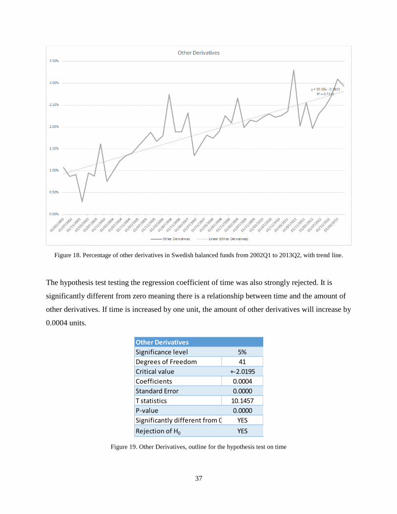
Figure 18. Percentage of other derivatives in Swedish balanced funds from 2002Q1 to 2013Q2, with trend line.

The hypothesis test testing the regression coefficient of time was also strongly rejected. It is

significantly different from zero meaning there is a relationship between time and the amount of

other derivatives. If time is increased by one unit, the amount of other derivatives will increase by

0.0004 units.

Figure 19. Other Derivatives, outline for the hypothesis test on time

Other Derivatives




Coefficients 0.0004


T statistics 10.1457

P-value 0.0000


Rejection of H0 YES

38

6.1.4 Unit Trusts

Figure 20. Unit Trusts, outline for the hypothesis test on the slope

The null hypothesis was rejected when measuring the difference between the mean of the first

and second half of all observations. Hence, there is a positive trend for the amount of unit trusts.

Unit Trusts


Mean 0.0062 0.0176

Variance 0.0000 0.0001

Observations 21 21






P-value 0.0000


Rejection of H0 YES

39

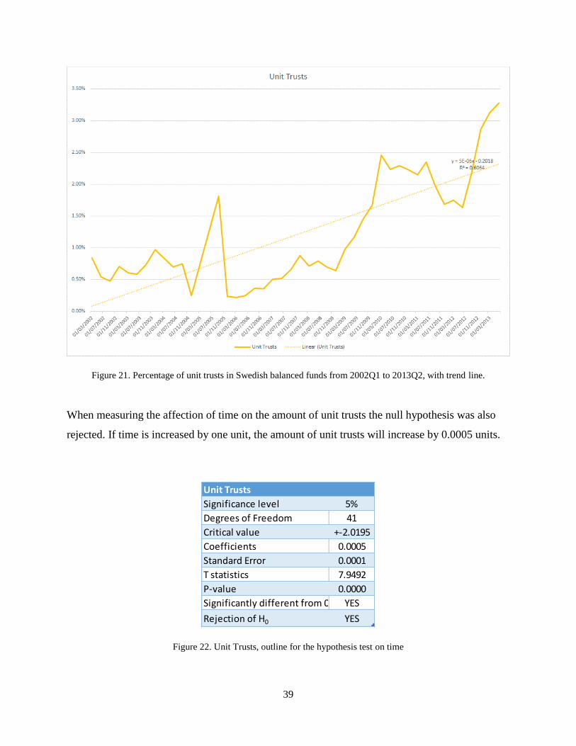
Figure 21. Percentage of unit trusts in Swedish balanced funds from 2002Q1 to 2013Q2, with trend line.

When measuring the affection of time on the amount of unit trusts the null hypothesis was also

rejected. If time is increased by one unit, the amount of unit trusts will increase by 0.0005 units.

Figure 22. Unit Trusts, outline for the hypothesis test on time

Unit Trusts




Coefficients 0.0005


T statistics 7.9492

P-value 0.0000


Rejection of H0 YES

40

6.2 Hypothesis test – Tactical Asset Allocation

The hypothesis test with null hypothesis β = 0, was testing if stock index, conjunction indicator or

interest rate had any significant impact on the short term allocation defined as tactical asset

allocation. In other words, the null hypothesis stated that the indices did not have any effect on

the way fund managers allocated assets. The results of the hypothesis test is presented below,

categorized by asset type.

6.2.1 Equities

Figure 23. Equities, outline for the hypothesis test on stock index, conjunction indicator and interest rates

According to the hypothesis test equities were not significantly different from zero when testing

stock index and conjunction indicator. Only the interest rate had a significant impact over time on

the amount of equities as a percentage of total assets. The regression coefficient for Stockholm

Interbank Rate 3M, is significantly different from 0, since the T-statistics is above the critical

value. The relationship between the variables is illustrated below, where one could see that the

line for equities are in a similar way as the line for Stockholm Interbank Rate 3M, but in a

dissimilar way from OMX Stockholm 30 Index and Swedbank PMI.

Equities OMX Stockholm 30 index Swedbank PMI Stockholm Interbank Rate 3M

Significance level 0.05 0.05 0.05

Degress of Freedom 39 39 39

Critical value +-2.0227 +-2.0227 +-2.0227

Coefficients -0.0038 0.0096 0.0397

Standard Error 0.0102 0.0230 0.0088

T statistics -0.3753 0.4166 4.4999

P-value 0.7094 0.6793 0.0001

Significantly different from 0 NO NO YES

Rejection of H0 NO NO YES

41

Figure 24. Development of the allocation of equities, OMX Stockholm 30 Index, Swedbank PMI and Stockholm

Interbank Rate 3M


Figure 25. Bonds and Convertibles, outline for the hypothesis test on stock index, conjunction indicator and interest

rates

0.00

20.00

40.00

60.00

80.00

100.00

120.00

140.00

160.00

180.00

Equities vs. indices


Bonds & Convertibles OMX Stockholm 30 index Swedbank PMI Stockholm Interbank Rate 3M



Critical value +-2.0227 +-2.0227 +-2.0227

Coefficients -0.3511 0.4626 -0.2008

Standard Error 0.0896 0.2024 0.0778

T statistics -3.9186 2.2858 -2.5815

P-value 0.0003 0.0278 0.0137

Significantly different from 0 YES YES YES

Rejection of H0 YES YES YES

42

For bonds and convertibles all variables were significantly different from zero. Although, OMX

Stockholm 30 Index and Stockholm Interbank Rate 3M had a negative regression coefficient,

meaning a negative relation. We could interpret the coefficient for OMX Stockholm 30 Index as

an increased by one unit, would lower the amount of equities with 0.3511 units. The relationship

between all variables is illustrated below.

Figure 26. Development of the allocation of bonds and convertibles, OMX Stockholm 30 Index, Swedbank PMI and

Stockholm Interbank Rate 3M

0.00

20.00

40.00

60.00

80.00

100.00

120.00

140.00

160.00

180.00

Bonds & Converitbles vs. indices

Bonds & Convertibles OMX Stockholm 30 index Swedbank PMI Stockholm Interbank Rate 3M

43

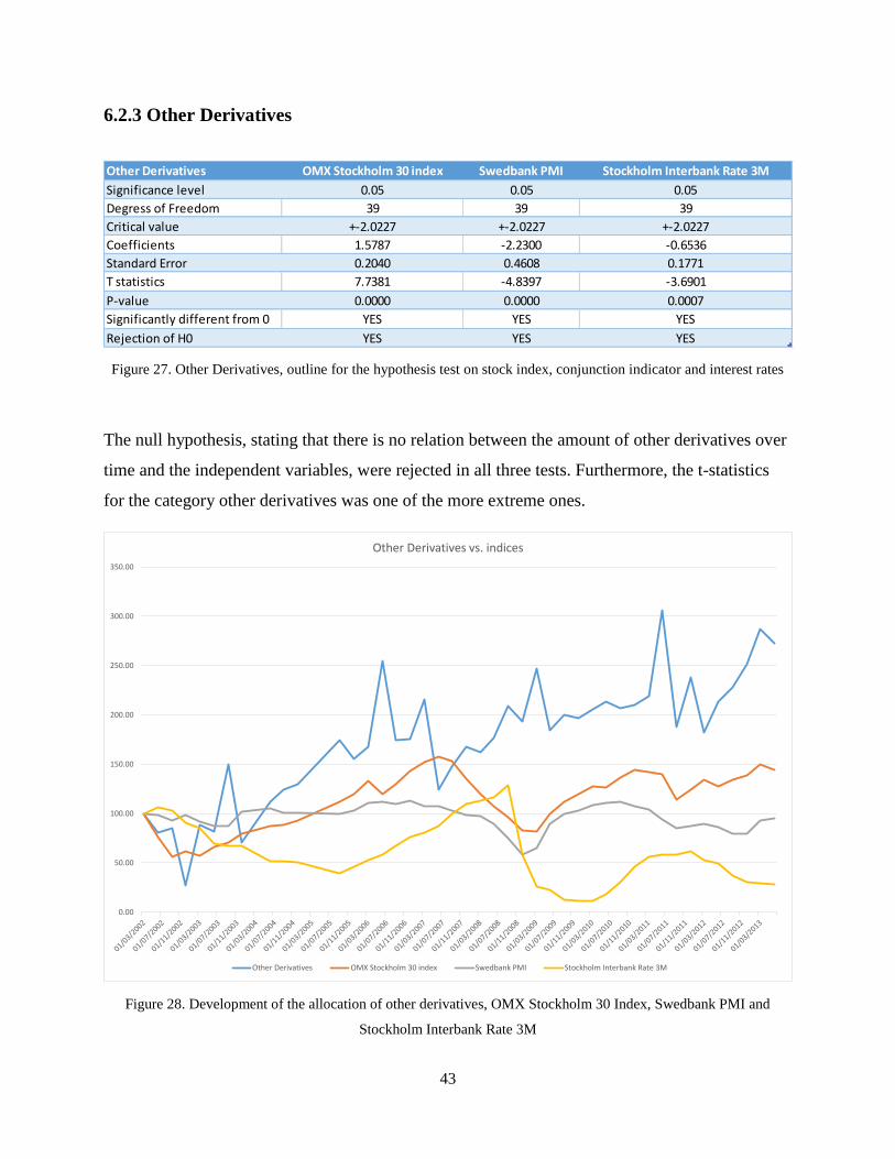
6.2.3 Other Derivatives

Figure 27. Other Derivatives, outline for the hypothesis test on stock index, conjunction indicator and interest rates

The null hypothesis, stating that there is no relation between the amount of other derivatives over

time and the independent variables, were rejected in all three tests. Furthermore, the t-statistics

for the category other derivatives was one of the more extreme ones.

Figure 28. Development of the allocation of other derivatives, OMX Stockholm 30 Index, Swedbank PMI and

Stockholm Interbank Rate 3M

Other Derivatives OMX Stockholm 30 index Swedbank PMI Stockholm Interbank Rate 3M



Critical value +-2.0227 +-2.0227 +-2.0227

Coefficients 1.5787 -2.2300 -0.6536

Standard Error 0.2040 0.4608 0.1771

T statistics 7.7381 -4.8397 -3.6901

P-value 0.0000 0.0000 0.0007



0.00

50.00

100.00

150.00

200.00

250.00

300.00

350.00

Other Derivatives vs. indices

Other Derivatives OMX Stockholm 30 index Swedbank PMI Stockholm Interbank Rate 3M

44

6.2.4 Unit Trusts

Figure 29. Unit Trusts, outline for the hypothesis test on stock index, conjunction indicator and interest rates

All variables tested in the category unit trust was significantly different from the null hypothesis.

The t-statistics for OMX Stockholm 30 index were positive, whereas the t-statistics for Swedbank

PMI and Stockholm Interbank Rate 3M were negative.

Unit Trusts OMX Stockholm 30 index Swedbank PMI Stockholm Interbank Rate 3M



Critical value +-2.0227 +-2.0227 +-2.0227

Coefficients 1.5675 -2.3623 -1.6284

Standard Error 0.4384 0.9902 0.3806

T statistics 3.5752 -2.3857 -4.2783

P-value 0.0010 0.0220 0.0001



0.00

50.00

100.00

150.00

200.00

250.00

300.00

350.00

400.00

450.00

Unit Trusts vs. indices

Unit Trusts OMX Stockholm 30 index Swedbank PMI Stockholm Interbank Rate 3M

45

Figure 30. Development of the allocation of unit trusts, OMX Stockholm 30 Index, Swedbank PMI and Stockholm

Interbank Rate 3M

6.3 Summary of results

Figure 31. Summary of all hypothesis tests, if they are rejected or not

Bond and convertibles were the only asset type where the null hypothesis was not rejected when

testing the long term trend - slope and time. Other derivatives and units trusts had a stronger

significant difference from zero, but even though equities did not have a strong trend, it was still

strong enough to be significantly different from zero.

When testing the stock index, conjunction indicator and interest rate, equities were the only asset

type where not all three trend-indicators were significantly different from zero. For all other asset

types the asset allocation and the indicators were following the same trend.

Equities Bonds & Convetibles Other Derivatives Unit Trusts

Strategic Asset Allocation

Slope YES NO YES YES

Time YES NO YES YES

Tactical Asset Allocation

OMX Stockholm 30 index NO YES YES YES

Swedbank PMI NO YES YES YES

Stockholm Interbank Rate 3M YES YES YES YES

46

7. ANALYSIS

In this chapter an analysis of the results will be presented. The initial problem will be

accounted for.

The most unexpected result from all the hypothesis tests done, were the fact that the hypothesis

test on tactical asset allocation showed that equities were not affected by the development of the

stock index. To recall the information from the results, that diagram presented in Chapter 6.2.1 is

presented again.

Figure 32. Development of the allocation of equities, OMX Stockholm 30 Index, Swedbank PMI and Stockholm

Interbank Rate 3M

0.00

20.00

40.00

60.00

80.00

100.00

120.00

140.00

160.00

180.00

Equities vs. indices


47

When analyzing this diagram, one could see that although the movement of equities (blue line) is

rather weak, it does follows the movement of OMX Stockholm 30 Index (red line) with a certain

lag. It would be reasonable to introduce a lag, because fund managers might not respond

immediately on occurrences in the market. Although, if a lag would have been introduced, there

would be an uncertainly in the time of the lag. While it is easy to identify a lag of equities from

OMX Stockholm 30 Index, it is also easy to identify another lag for the equities and Stockholm

Interbank Rate 3M. Therefore, if a shorter lag would have been chosen it would have benefited

the Stockholm Interbank Rate 3M and if a longer lag would have been chosen it would have

benefited the OMX Stockholm 30 Index. Not having any lag makes the thesis more neutral, but

in this case it also affected the results negatively.

By looking at the diagrams over the compiled data of asset allocation, it was rather obvious the

majority of the null hypothesis would be rejected. For many of the asset types, except for bonds

and convertibles, there was a strong trend in the allocation.

The real issue of this essay was not whether the hypothesis tests were rejected or not, it was

rather how to interpret the output and results. Before compiling the data, a definition of strategic

and tactical asset allocation was done. The strategic asset allocation was defined as the long term

trend and the tactical asset allocation as the deviation from this trend.

When bonds and convertibles did not have a significant trend and was not significantly affected

by time, there was according to the initial definition no strategic asset allocation, since there was

no long term trend. Despite this, one should take into consideration that an interpretation of the

results as without strategic asset allocation, might be misleading because the strategic asset

allocation might have been fixed for bonds and convertibles.

48

8. CONCLUSION

In this chapter the initial problem will be answered by a summary of the results and the

analysis.

The initial problem of this thesis was as followed:

Are strategic and tactical asset allocation used within Swedish balanced funds in a way that

trends could be identified?

The short answer to the question is yes, it is.

In this thesis we have seen that the strategic allocation changes over time and there are significant

long term trends for three out of four asset classes. Over time, the amount of equities has

decreased and the amount of other derivatives and unit trusts have increased.

According to the definition of tactical asset allocation as a deviation from the long term trend, it

is concluded that tactical asset allocation has been used within Swedish balanced funds. The

tactical asset allocation is a function of stock index, conjunction indicator and interest rates for

almost all asset types. Although, for equities, there is a certain lag in the allocation.

In the analysis a discussion about the definition of strategic and tactical asset allocation was also

presented, in order to highlight the implications of defining quantitative data.

9. FURTHER RESEARCH

Suggestions for further research is presented in this chapter.

This thesis was done on a quantitative methodological approach which has given a general view,

based on facts and not opinions. Although, a suggestion to further research will be a qualitative

analysis. A comparison of the results is encouraged in order to get a full picture of the usage of

strategic and tactical asset allocation within Swedish balanced funds.

49

This thesis did not analyze specific occurrences and their affection of the asset allocation, for

example how the amount of equities was affected by the finical crisis in 2008. A research on the

markets affections of investment strategies will also be encouraged.

10. BIBLIOGRAPHY

10.1 Books

Backman Jarl, Rapporter och Uppsatser, Studentlitteratur AB, Lund, 2010

Bodie Zvi, Kane Alex, Marcus Alan, Investments and Portfolio Management, ninth edition,

McGraw Hill, New York, 2011

Byström Hans, Finance – Markets, Instruments and Investments, Studentlitteratur, Lund, 2007

Dahlström Karin, Från datainsamling till rapport, femte upplagan, Studentlitteratur, 2001

Minto Barbara, The pyramid principle. Logic in writing and thinking, third edition, Pearson

Education, Essex, 2009

Newbold Paul, Carlson William, Thorne Betty, Statistics for Business and Economics, eight

edition, Pearson, USA, 2013

Wiederheim-Paul Finn, Eriksson Lars Torsten, Att utreda, forska och rapportera, Liber ekonomi,

Malmö, 1999

50

10.2 Journal articles

Avdic Anders, Riktlinjer för rapportering, version 2,8, Örebro Universitet

Brennan Michael, Schwarz Eduardo, Lagnado Ronald, ‘Strategic Asset Allocation’, Journal of

Economic Dynamics & Control, vol. 21, 1997

Campbell John, Chan Yeung Lewis, Viceira Luis M, ‘A multivariate model of strategic asset

allocation’, Journal of Financial Economics’, vol. 67, January 2002

Campbell John, Viceira Luis M, Strategic Asset Allocation: Portfolio Choice for Long Term

Investors, Oxford University Press: 2002

Erlwein Christina, Mamon Rogemar, Davidson Matt, ‘An examination of HHM-based

investment strategies for asset allocation’, Applied Stochastic Models in Business and Industry,

December 2009

Hood Randolph L, ‘Determinants of Portfolio Performance - 20 years later’, Financial Analysts

Journal, 2005

Hörte Sven-Åke, Hur kan man ge struktur åt rapporter och uppsatser?, Luleå Tekniska

Universitet, Avdelningen för Industriell Organisation

Ibbotson Roger G, Kaplan Paul D, Does Asset Allocation Policy Explain 40,90 or 100 percent of

Performance, Financial Analysts Journal, Jan/Feb 2000

Idzorek Tomas, Strategic Asset Allocation and Commodities, Ibbotson, Chicago, 2006

Jahnke William, ‘The Asset Allocation Hoax’, Financial Design – White paper, vol. 1, February

1997

51

Statman Meir, The 96,3 % Question of Financial Advisors, 2000

Sui Tak Kuen, ‘Long-term strategic asset allocation with inflation risk and regime switching’,

Quantitative Finance, vol. 11, May 2009

10.3 Electronic sources

Avanza – OMXS30


2014-04-19

Investopedia - Asset Allocation


2014-03-31

Investopedia - Strategic Asset Allocation


2014-03-31

ISIN


2014-03-31

Morningstar - Balanced Fund


2014-02-06

Morningstar – Category


2014-03-31







52

National bank of Sweden – Explanation of the series

http://www.riksbank.se/sv/Rantor-och-valutakurser/Forklaring-till-serierna/Svenska-

marknadsrantor/

2014-04-19

Nysparande och fondförmögenhet 2014


2014-04-19

Swedbank – PMI

http://www.swedbank.se/om-

swedbank/analyser/samhallsekonomi/inkopschefsindex/inkopschefsindex,-mal-och-

metodik/index.htm

2014-04-19

Swedish Financial Supervisory Authority – About fund holdings


2014-03-31

Swedish Financial Supervisory Authority – Fund holdings


2014-03-31

Swedish Financial Supervisory Authority – Registered companies not under the supervisory of FI


2014-03-31










53

11. APPENDIX

11.1 Regression analysis – strategic asset allocation

11.1.1 Equities

Equities, regression analysis on the difference on the slope

Equities, regression analysis on time

t-Test: Two-Sample Assuming Equal Variances

Equities

Variabel 1 Variabel 2

Mean 0.9041 0.8910

Variance 0.0002 0.0004

Observations 21 21



df 40

t Stat 2.4714

P(T<=t) one-tail 0.0089

t Critical one-tail 1.6839

P(T<=t) two-tail 0.0178

t Critical two-tail 2.0211

SUMMARY OUTPUT


Multiple R 0.4446

R Square 0.1977




ANOVA


Regression 1.0000 0.0029 0.0029 10.1006 0.0028

Residual 41.0000 0.0119 0.0003

Total 42.0000 0.0149

CoefficientsStandard Errort Stat P-value Lower 95%Upper 95%Lower 95.0%Upper 95.0%

Intercept 0.9118 0.0054 168.8841 0.0000 0.9009 0.9227 0.9009 0.9227

t -0.0006 0.0002 -3.1781 0.0028 -0.0010 -0.0002 -0.0010 -0.0002

54


Bonds and Convertibles, regression analysis on the difference on the slope

Bonds and Convertibles, regression analysis on time


Bonds & Convertibles


Mean 0.0753 0.0681

Variance 0.0002 0.0001

Observations 21 21



df 40

t Stat 1.7387





SUMMARY OUTPUT


Multiple R 0.2940

R Square 0.0864




ANOVA


Regression 1.0000 0.0007 0.0007 3.8798 0.0557

Residual 41.0000 0.0070 0.0002

Total 42.0000 0.0077


Intercept 0.0790 0.0041 19.0479 0.0000 0.0706 0.0874 0.0706 0.0874

t -0.0003 0.0001 -1.9697 0.0557 -0.0006 0.0000 -0.0006 0.0000

55

11.1.3 Other derivatives

Other Derivatives, regression analysis on the difference on the slope

Other Derivatives, regression analysis on time


Other Derivatives


Mean 0.0144 0.0232

Variance 0.0000 0.0000

Observations 21 21



df 40

t Stat -5.8397





SUMMARY OUTPUT


Multiple R 0.8457

R Square 0.7151




ANOVA


Regression 1.0000 0.0013 0.0013 102.9351 0.0000

Residual 41.0000 0.0005 0.0000

Total 42.0000 0.0019


Intercept 0.0089 0.0011 7.7898 0.0000 0.0066 0.0112 0.0066 0.0112

t 0.0004 0.0000 10.1457 0.0000 0.0003 0.0005 0.0003 0.0005

56

11.1.4 Unit trusts

Unit Trusts, regression analysis on the difference on the slope

Unit Trusts, regression analysis on time


Unit Trusts


Mean 0.0062 0.0176

Variance 0.0000 0.0001

Observations 21 21



df 40

t Stat -6.5221





SUMMARY OUTPUT


Multiple R 0.7788

R Square 0.6065




ANOVA


Regression 1.0000 0.0019 0.0019 63.1898 0.0000

Residual 41.0000 0.0012 0.0000

Total 42.0000 0.0031


Intercept 0.0003 0.0017 0.1913 0.8492 -0.0032 0.0038 -0.0032 0.0038

t 0.0005 0.0001 7.9492 0.0000 0.0004 0.0006 0.0004 0.0006

57

11.2 Regression analysis – tactical asset allocation

11.2.1 Equities

Equities, regression analysis on stock index, conjunction indicator and interest rates


SUMMARY OUTPUT


Multiple R 0.6052

R Square 0.3663




ANOVA


Regression 3.0000 66.4665 22.1555 7.5148 0.0004

Residual 39.0000 114.9816 2.9482

Total 42.0000 181.4481

Coefficients Standard Errort Stat P-value Lower 95%Upper 95%Lower 95.0%Upper 95.0%

Intercept 96.2039 2.2239 43.2590 0.0000 91.7056 100.7021 91.7056 100.7021

OMX Stockholm 30 index -0.0038 0.0102 -0.3753 0.7094 -0.0244 0.0168 -0.0244 0.0168

Swedbank PMI 0.0096 0.0230 0.4166 0.6793 -0.0369 0.0560 -0.0369 0.0560

Stockholm Interbank Rate 3M 0.0397 0.0088 4.4999 0.0001 0.0219 0.0576 0.0219 0.0576

58

Bonds and convertibles, regression analysis on stock index, conjunction indicator and interest rates

11.2.3 Other derivatives

SUMMARY OUTPUT


Multiple R 0.5746

R Square 0.3302




ANOVA


Regression 3.0000 4398.4679 1466.1560 6.4093 0.0012

Residual 39.0000 8921.3868 228.7535

Total 42.0000 13319.8547


Intercept 102.1678 19.5893 5.2155 0.0000 62.5448 141.7908 62.5448 141.7908

OMX Stockholm 30 index -0.3511 0.0896 -3.9186 0.0003 -0.5323 -0.1699 -0.5323 -0.1699

Swedbank PMI 0.4626 0.2024 2.2858 0.0278 0.0533 0.8719 0.0533 0.8719

Stockholm Interbank Rate 3M -0.2008 0.0778 -2.5815 0.0137 -0.3581 -0.0435 -0.3581 -0.0435

SUMMARY OUTPUT


Multiple R 0.8442

R Square 0.7126




ANOVA


Regression 3.0000 114709.0520 38236.3507 32.2404 0.0000

Residual 39.0000 46253.0417 1185.9754

Total 42.0000 160962.0937


Intercept 251.2668 44.6038 5.6333 0.0000 161.0471 341.4865 161.0471 341.4865

OMX Stockholm 30 index 1.5787 0.2040 7.7381 0.0000 1.1660 1.9914 1.1660 1.9914

Swedbank PMI -2.2300 0.4608 -4.8397 0.0000 -3.1620 -1.2980 -3.1620 -1.2980


59

Other derivatives, regression analysis on stock index, conjunction indicator and interest rates

11.2.4 Unit trusts

Unit trusts, regression analysis on stock index, conjunction indicator and interest rates

SUMMARY OUTPUT


Multiple R 0.7194

R Square 0.5175




ANOVA


Regression 3.0000 229124.3891 76374.7964 13.9447 0.0000

Residual 39.0000 213601.6923 5476.9665

Total 42.0000 442726.0814


Intercept 295.6958 95.8527 3.0849 0.0037 101.8155 489.5761 101.8155 489.5761

OMX Stockholm 30 index 1.5675 0.4384 3.5752 0.0010 0.6807 2.4543 0.6807 2.4543

Swedbank PMI -2.3623 0.9902 -2.3857 0.0220 -4.3652 -0.3595 -4.3652 -0.3595


a study of two investment strategies within swedish...

Documents