a study of impacts of coupled model initial shocks and ... · a study of impacts of coupled model...

A Study of Impacts of Coupled Model Initial Shocks and State–Parameter Optimizationon Climate Predictions Using a Simple Pycnocline Prediction Model

S. ZHANG

NOAA/GFDL, Princeton University, Princeton, New Jersey

(Manuscript received 7 December 2010, in final form 16 June 2011)

ABSTRACT

A skillful decadal prediction that foretells varying regional climate conditions over seasonal–interannual

to multidecadal time scales is of societal significance. However, predictions initialized from the climate-

observing system tend to drift away from observed states toward the imperfect model climate because of the

model biases arising from imperfect model equations, numeric schemes, and physical parameterizations, as

well as the errors in the values of model parameters. Here, a simple coupled model that simulates the fun-

damental features of the real climate system and a ‘‘twin’’ experiment framework are designed to study the

impact of initialization and parameter optimization on decadal predictions. One model simulation is treated

as ‘‘truth’’ and sampled to produce ‘‘observations’’ that are assimilated into other simulations to produce

observation-estimated states and parameters. The degree to which the model forecasts based on different

estimates recover the truth is an assessment of the impact of coupled initial shocks and parameter optimi-

zation on climate predictions of interests. The results show that the coupled model initialization through

coupled data assimilation in which all coupled model components are coherently adjusted by observations

minimizes the initial coupling shocks that reduce the forecast errors on seasonal–interannual time scales.

Model parameter optimization with observations effectively mitigates the model bias, thus constraining the

model drift in long time-scale predictions. The coupled model state–parameter optimization greatly enhances

the model predictability. While valid ‘‘atmospheric’’ forecasts are extended 5 times, the decadal predictability

of the ‘‘deep ocean’’ is almost doubled. The coherence of optimized model parameters and states is critical to

improve the long time-scale predictions.

1. Introduction

Because of the imperfect model structures such as model

equations, numeric schemes, and physical parameteriza-

tions, as well as the errors in the values of model param-

eters, a coupled climate model is biased so that the model

climate tends to drift away from the real world (Delworth

et al. 2006; Collins et al. 2006). To obtain the initial con-

ditions from which a model prediction can be started with

the observed state, the measured data in the climate ob-

serving system are assimilated into a coupled model to

estimate the historical and present climate states. How-

ever, due to the existence of model bias, the climate pre-

diction initialized from the observing system also tends

to drift away from the observed states toward the imper-

fect model climate (Smith et al. 2007).

Traditionally, one tries to mitigate the bias in initial

conditions through a statistical method (e.g., Dee and Silva

1998; Dee 2005; Cherupin et al. 2005) or only assimilating

(restoring) anomalies rather than the full values into a

model (Smith et al. 2007; Keenlyside et al. 2008). Directly

estimating model parameters using observations through

expanding the adjustable variables of assimilation to in-

clude parameters is another approach to limit model bias

(e.g., Anderson 2001; Annan and Hargreaves 2004; Annan

et al. 2005; Aksoy et al. 2006a,b; Evensen 2007; Hansen

and Penland 2007; Kondrashov et al. 2008; Tong and Xue

2008a,b; Yang and DelSole 2009; DelSole and Yang 2010).

However, without modifying the traditional data assimi-

lation procedure, effective parameter estimation is usually

difficult within a coupled data assimilation (CDA) system

in which multiple time scale model components are in-

vloved, even though it is theoretically promising. In gen-

eral, unlike traditional state estimation where the system

states are directly adjusted by observations of states, with-

out direct observations and prognostic equations, parame-

ter estimation completely relies on the covariance between

Corresponding author address: Shaoqing Zhang, GFDL/NOAA,

Princeton University, P.O. Box 308, Princeton, NJ 08542.

E-mail: [email protected]

6210 J O U R N A L O F C L I M A T E VOLUME 24

DOI: 10.1175/JCLI-D-10-05003.1

a parameter and the model state for projecting the ob-

servational information of state variables onto the pa-

rameter being estimated. The examination using a simple

coupled model found that to establish a signal-dominant

state–parameter covariance, the coupled model ensem-

ble is required to be sufficiently constrained by observa-

tions that may come from different system components

with different time scales, and otherwise the noisy co-

variance could bring the parameter toward an erroneous

value (Zhang et al. 2011). This difficulty is relaxed by the

proposed assimilation scheme with enhancive parame-

ter correction. In that scheme, the signal-dominant co-

variance between a parameter and the model state

facilitates parameter correction when coupled state es-

timation reaches a ‘‘quasi equilibrium’’ where the un-

certainty of model states has been sufficiently constrained

by observations and it therefore becomes more con-

trolled by parameter errors. Once the observation-based

parameter optimization is facilitated, numerical climate

prediction based on a biased coupled model becomes

a ‘‘coupled state–parameter optimization problem’’ rather

than only a ‘‘state initial value problem.’’ How much of the

model drift in decadal predictions can be constrained by

the coupled model state–parameter optimization? A

simple pycnocline prediction model that characterizes

the seasonal–interannual (SI) to decadal variability of the

climate system and a ‘‘twin’’ experiment framework are

designed to address this question. In the twin experiment

framework, one model simulation is treated as ‘‘truth’’ and

is sampled to produce ‘‘observations,’’ and then the syn-

thetic ‘‘observations’’ are assimilated into other simula-

tions to produce observation-optimized model states or

observation-optimized model states and parameters.

The degree to which the model forecasts based on dif-

ferent assimilation results recover the truth is used to

assess the impact of different coupled initialization

schemes as well as observation-optimized model pa-

rameters on climate predictions.

The motivation of this study is mainly to present the

impacts of minimized initial coupling shocks in coupled

data assimilation on climate predictions with various time

scales, and as the whole topic of climate predictability

enhancement, they are linked with the impact of coupled

model state-parameter optimization. Although some of

the preliminary results on the impact of observation-

optimized model parameters on decadal prediction from

this study have been briefly reported in a letter (Zhang

2011), here the author still presents the details of the

impact of coupled model state–parameter optimization

with observations on various time-scale climate predic-

tions. After describing the construction of the simple

pycnocline prediction model, section 2 first gives a brief

description for the ensemble filter and then presents the

design of the twin experiment framework, both of which

will be used throughout the paper for state estimation and

parameter optimization, as well as the prediction assess-

ment. In the twin experiment framework, an assimilation

model is set with a set of erroneous values for all model

parameters while the ‘‘truth’’ model with a set of ‘‘stan-

dard’’ parameter values defines the ‘‘true’’ solution for the

estimation and prediction problem, and the observations

are samples of the true solution. Section 3 examines the

impact of minimized initial shocks on various time-scale

climate predictions using the coupled data assimilation

procedure. Section 4 examines the impact of the coupled

model state–parameter optimization on long time-scale

climate predictions. Conclusions and discussions are

given in section 5.

2. Methodology

a. A simple pycnocline prediction model

Because of the complex physical processes and huge

computational cost involved, it is not convenient to use

a coupled general circulation model (CGCM) to clearly

address the impact of coupled model initial shocks and

state-parameter optimization on climate predictions. In-

stead, as the first step of the studies on this research topic,

the author constructs a simple decadal prediction model

in this section. For the problem that is concerned, this

simple decadal prediction model shall share the fol-

lowing fundamental features of a CGCM:

1) the ocean variability is a consequence of the response

of the slow ocean to the fast atmosphere, and in

return the air–sea interaction can modify the statis-

tical character of the atmosphere;

2) while much slower deep ocean is driven by the upper

ocean, as the feedback it also modulates low-frequency

variability of the upper ocean so as to impact on the

atmosphere through the air-sea interaction; and

3) a perturbation on any parameter of each model

component can change the model solution.

The construction starts from the simple coupled model

developed in the previous study (Zhang et al. 2011) in

which a slowly-varying variable w is coupled with the

Lorenz’s 3-variable chaotic model (Lorenz 1963) to sim-

ulate the interaction of the fast atmosphere with the slow

upper ocean:

_x1 5 2sx1 1 sx2

_x2 5 2x1x3 1 (1 1 c1w)kx1 2 x2

_x3 5 x1x2 2 bx3

Om_w 5 c2x2 2 Odw 1 Sm 1 Ss cos(2pt/Spd), (1)

1 DECEMBER 2011 Z H A N G 6211

where an overdot denotes time tendency; x1, x2, and x3

are the high-frequency variables of the atmosphere with

the original s, k, and b parameters and their standard

values 9.95, 28, and 8/3, which sustain the chaotic nature

of the atmosphere. For w, except for a forcing term from

the atmosphere (c2x2), the simplest slab ocean only con-

sists of a linear damping term 2Od w and an imposed

external forcing. An important feature of w is that it must

have a much slower time scale than the atmosphere, which

can be obtained by requiring a much larger heat capacity

than the damping rate, that is, Om� Od. For example,

the values of (10, 1) for (Om, Od) define the oceanic time

scale as ;O(10), 10 times of the atmospheric time scale

;O(1). Also simply setting the external forcing as Sm 1

Ss cos(2pt/Spd) simulates the constant and seasonal

forcings for the ‘‘climate’’ system so that the ‘‘ocean’’ is

recharged when it is damped, where Spd defines the pe-

riod of seasonal cycle. The Spd is chosen as 10 so that the

period of the forcing is comparable with the oceanic time

scale, defining the time scale of the model seasonal cycle.

The parameters Sm and Ss define the magnitudes of

the annual mean and seasonal cycle of the forcings, which

are not sensitive to the model construction and set as 10

and 1, respectively. The coupling between the fast atmo-

sphere and slow ocean is realized by choosing the values of

the coupling coefficients c1 and c2, with c1 representing the

oceanic forcing on the atmosphere, and c2 representing the

atmospheric forcing on the ocean. Here, the multiplicative

way of ocean to force the atmosphere allows the coupling

forcing to produce some modulation for the atmospheric

attractor, and for simplicity, only one oceanic forcing as

a multiplicative forcing is kept in the x2 equation. Exper-

iments show that the coupled system is robust with respect

to c2 but becomes unstable when c1 is much larger than 0.1,

so c1 and c2 are set as 0.1 and 1, respectively. A set of

standard parameter values (s, k, b, c1, c2, Om, Od, Sm, Ss,

Spd) 5 (9.95, 28, 8/3, 1021, 1, 1, 10, 10, 1, 10) was used to

simulate the fundamental character of the coupled climate

system in tropics. Forced by the fluxes of the ‘‘chaotic’’

atmosphere, the slow ocean w generates its internal

‘‘seasonal–interannual’’ variability with a 10-times larger

time scale than that of the atmospheric variables x1,2,3

[usually about 1 nondimensional time unit (TU)]. More-

over, the forcing from the ocean to the atmosphere alters

the centers of the lobe of the atmospheric attractor.

The other important component of the simple de-

cadal prediction model is a simple pycnocline predictive

model derived from the two-term balance model of

the zonal–time mean pycnocline (Gnanadesikan 1999).

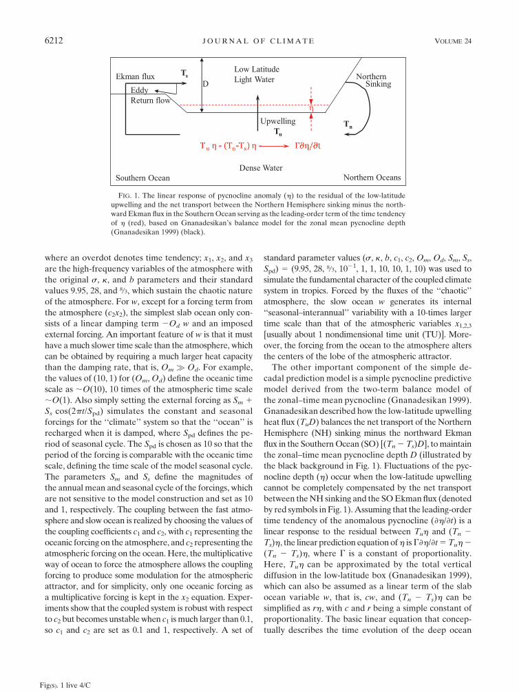
Gnanadesikan described how the low-latitude upwelling

heat flux (TuD) balances the net transport of the Northern

Hemisphere (NH) sinking minus the northward Ekman

flux in the Southern Ocean (SO) [(Tn 2 Ts)D], to maintain

the zonal–time mean pycnocline depth D (illustrated by

the black background in Fig. 1). Fluctuations of the pyc-

nocline depth (h) occur when the low-latitude upwelling

cannot be completely compensated by the net transport

between the NH sinking and the SO Ekman flux (denoted

by red symbols in Fig. 1). Assuming that the leading-order

time tendency of the anomalous pycnocline (›h/›t) is a

linear response to the residual between Tuh and (Tn 2

Ts)h, the linear prediction equation of h is G›h/›t 5 Tuh 2

(Tn 2 Ts)h, where G is a constant of proportionality.

Here, Tuh can be approximated by the total vertical

diffusion in the low-latitude box (Gnanadesikan 1999),

which can also be assumed as a linear term of the slab

ocean variable w, that is, cw, and (Tn 2 Ts)h can be

simplified as rh, with c and r being a simple constant of

proportionality. The basic linear equation that concep-

tually describes the time evolution of the deep ocean

FIG. 1. The linear response of pycnocline anomaly (h) to the residual of the low-latitude

upwelling and the net transport between the Northern Hemisphere sinking minus the north-

ward Ekman flux in the Southern Ocean serving as the leading-order term of the time tendency

of h (red), based on Gnanadesikan’s balance model for the zonal mean pycnocline depth

(Gnanadesikan 1999) (black).

Fig(s). 1 live 4/C


pycnocline becomes G›h/›t 5 cw 2 rh. The term 2rh

also represents the damping mechanism, and for this

simple system, only accounting for the ocean’s viscosity,

we set r 5 Od where Od is the damping coefficient of the

slab ocean variable w. The ratio of G and Od determines

the time scale of variations of h, for example, a value of

100 for G defining 10 ‘‘seasonal’’ cycles of w (a model de-

cade) as the typical time scale of h variability. To sim-

ulate the effects of the nonlinear advection in the upper

and deep oceans, the nonlinear terms are introduced

into w and h equations. Finally, the conceptual pycno-

cline prediction model takes the form as

_x1 5 2sx1 1 sx2

_x2 5 2x1x3 1 (1 1 c1w)kx1 2 x2

_x3 5 x1x2 2 bx3

Om_w 5 c2x2 1 c3h 1 c4wh 2 Odw 1 Sm

1 Ss cos(2pt/Spd)

G _h 5 c5w 1 c6wh 2 Odh, (2)

which includes 5 model variables (x1, x2, and x3 for the

atmosphere, w for the slab ocean, and h for the deep

ocean pycnocline) and 5 new parameters. For the equa-

tion of w, c3 and c4 represent the linear forcing of the

deep ocean and the nonlinear interaction of the upper

and deep oceans, and we set their magnitude order smaller

than that of c2 [note c2 ; O(1)] to retain the leading-order

role of the atmosphere–ocean coupling for the slab ocean.

For h, we set c5 ; O(1) to retain the leading-order role of

the linear response of the deep ocean to the upper ocean.

Also assuming that the nonlinearity of the deep ocean is

weaker than that of the upper ocean, the order of c6 is set

smaller than that of c4. Given these constraints, experi-

ments show that the model construction is robust and not

quite sensitive to the values of these coefficients, and we

choose c3 and c4 ; O(1022) and c6 ; O(1023).

Using a leapfrog time differencing scheme (Dt 5 0.01)

with a Robert–Asselin time filter (Robert 1969; Asselin

1972) (denote the time filtering coefficient as g 5 0.25),

the model is first spun up for 104 TUs starting from (x1, x2,

x3, w, h) 5 (0, 1, 0, 0, 0) with the values of 16 model pa-

rameters described above, that is, (s, k, b, c1, c2, Om, Od,

Sm, Ss, Spd, G, c3, c4, c5, c6, g) 5 (9.95, 28, 8/3, 1021, 1, 1, 10,

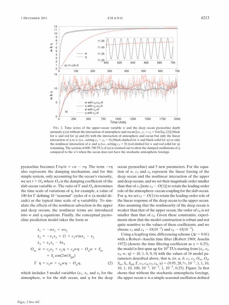
10, 1, 10, 100, 1022, 1022, 1, 1023, 0.25). Figure 2a first

shows that without the stochastic atmospheric forcings,

the upper ocean w is a simple seasonal oscillation defined

FIG. 2. Time series of the upper-ocean variable w and the deep ocean pycnocline depth

anomaly h (a) without the interaction of atmosphere and ocean [i.e., c1 5 c2 5 0 in Eq. (2)] (black

for w and red for h) and (b) with the interaction of atmosphere and ocean but only the linear

interaction of h to w (i.e., setting c4 5 c6 5 0) (black-dashed for w and black-solid for h) or only

the nonlinear interaction of w and h (i.e., setting c3 5 0) (red-dashed for w and red-solid for h)

remaining. The section of 600–700 TUs of (a) is zoomed out to show the damped oscillations of h

compared to the w’s when the ocean does not have the stochastic atmospheric forcings.

Fig(s). 2 live 4/C


by Spd, and the deep ocean h is a damped oscillation

based on the input of w. With the atmospheric forcings,

the model then is run only with the linear interaction of w

and h (i.e., setting c4 5 c6 5 0) or only with the nonlinear

interaction of w and h (i.e., setting c3 5 0), and results are

shown in Fig. 2b. From Fig. 2b, it is clear that the linear

terms in the w and h equations respond to the atmo-

spheric forcings to create interannual to decadal scale

oscillations for the deep ocean, while the nonlinear terms

tend to modulate longer time scale variability.

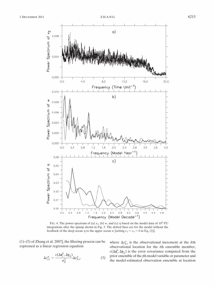
An interesting aspect of the model is the influence of

the h–w interaction on the upper ocean and atmosphere.

Figs. 3 and 4 show the variability of the ocean and at-

mosphere with or without the feedback of h on the up-

per ocean by setting c3 and c4 as 1022 or 0 (Fig. 3) as well

as the corresponding power spectrum (Fig. 4). It is clear

that the feedback of h to w helps transfer the energy of

deep ocean from the subdecadal scales to decadal and

interdecadal scales. The model variability shows that the

upper ocean includes high-frequency and low-frequency

variability, and the upper ocean can be transient by the

more slowly varying deep ocean so that the deep ocean has

an impact on the atmosphere attractor through the air–

sea interaction. Namely, the simple model simulates the

fundamental features of the real world climate system—

the upper ocean interacts with the transient atmospheric

attractor above and the deep ocean below—the decadal

and longer time scale variability of deep ocean has the

impact on the transient atmospheric attractor through the

feedbacks of the upper ocean to the atmosphere.

b. Coupled data assimilation with an ensemble filterfor state and parameter estimations

An ensemble filter uses the error statistics evaluated

from ensemble model integrations, such as error covari-

ances between model states, to extract observational in-

formation to adjust the model ensemble for state estimation

(e.g., Evensen 1994; Anderson 2001; Hamill et al. 2001). The

ensemble-evaluated covariances between model states and

model parameters can also be used to estimate the model

parameters (e.g., Anderson 2001; Annan and Hargreaves

2004; Annan et al. 2005; Aksoy et al. 2006a,b; Evensen

2007; Hansen and Penland 2007; Kondrashov et al. 2008;

Tong and Xue 2008b; Yang and DelSole 2009; DelSole

and Yang 2010). Based on the two-step ensemble ad-

justment Kalman filter (EAKF; Anderson 2001; 2003;

Zhang and Anderson 2003; Zhang et al. 2007), once the

ensemble observation increment is computed [see Eqs.

FIG. 3. Time series of (a) the upper-ocean variable w (dotted) and the deep ocean pycnocline

depth anomaly h (solid) and (b) the atmospheric variable x2 produced by Eq. (2) starting from

the initial conditions (x1, x2, x3, w, h) 5 (0, 1, 0, 0, 0). The dotted (solid) green lines in (a) [for w

(h)] and the dotted black line in (b) (for x2) are the results of the model without the upper-

ocean and deep ocean coupling [i.e., setting c3 5 c4 5 0 in Eq. (2), which degrades to the upper

ocean and atmosphere coupled model described by Eq. (1)]. The solid-green line in (a) is the

result of integrating the h equation that only depends on the w values from the upper ocean and

atmosphere coupled model without any feedback of h to w.

Fig(s). 3 live 4/C


(1)–(5) of Zhang et al. 2007], the filtering process can be

expressed as a linear regression equation:

Dzuj,i 5

c(Dzpj , Dyk)

s2k

Dyok,i, (3)

where Dyok,i is the observational increment at the kth

observational location for the ith ensemble member,

c(Dzpj , Dy

k) is the error covariance computed from the

prior ensemble of the jth model variable or parameter and

the model-estimated observation ensemble at location

FIG. 4. The power spectrum of (a) x2, (b) w, and (c) h based on the model data of 104-TU

integrations after the spinup shown in Fig. 3. The dotted lines are for the model without the

feedback of the deep ocean h to the upper ocean w [setting c3 5 c4 5 0 in Eq. (2)].


k, and sk is the standard deviation of the model en-

semble at location k. the quantity Dzj,i is the adjustment

amount for the jth model variable or parameter of the

ith ensemble member.

The application of Eq. (3) to the state variables (re-

placing zj by the state vector xj with j as the index of

model state variables) of a coupled model when reliable

observations are available implements CDA for state

estimation in a straightforward manner (Zhang et al.

2007). However, effective parameter estimation is usu-

ally difficult before the uncertainty of model states in

CDA has been sufficiently constrained by observations.

To have an enhancive parameter correction with obser-

vational information, the application of Eq. (3) for cou-

pled parameter estimation (replacing zj by the parameter

ensemble vector bl with l as the index of model param-

eters) has to be delayed until the state estimation reaches

a quasi-equilibrium, where the errors of model states be-

come mainly contributed from model parameter errors.

With the modified data assimilation scheme, coupled data

assimilation with parameter optimization (CDAPO) is fa-

cilitated using the covariance between a parameter and

the model state when the state estimation of CDA rea-

ches quasi equilibrium. More discussion about the ap-

plication of the CDAPO scheme to the simple pycnocline

prediction model developed in section 2a will be given in

section 4, where the impact of observation-optimized

parameters on decadal-scale climate predictions is ad-

dressed through twin experiments described below.

c. Twin experiment setup

The decadal prediction model with the standard pa-

rameter values described in section 2a produces the true

solution for the assimilation–prediction problem, called

truth. The observations are samples of the truth model

states after the spinup of 104 TUs. A random noise is su-

perimposed on the values of x1,2,3 and w at an interval

of 0.1 and 0.4 TU, respectively. The observational fre-

quency simulates the feature of the real climate observing

system in which the atmospheric observations are avail-

able more frequently (subdaily) than the oceanic obser-

vations (roughly-daily). Also, to simulate the lack of deep

ocean measurements in the real observing system, no

observation is available for h. The standard deviation of

observational errors is 2 for x1,2,3 and 0.5 for w. A biased

assimilation–prediction model in which all parameters

are set to have a 10% overestimated error from their

standard values is used to assimilate the observations

into the model and predict the truth by traditional CDA

or CDAPO schemes. As the truth model does, starting

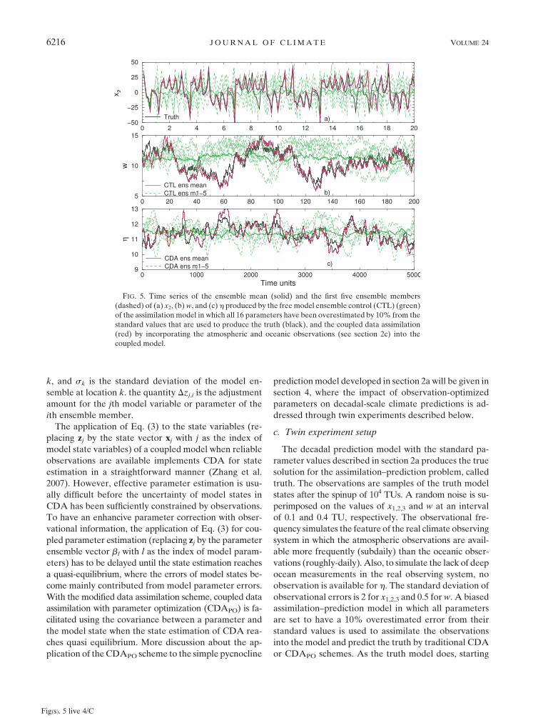
FIG. 5. Time series of the ensemble mean (solid) and the first five ensemble members

(dashed) of (a) x2, (b) w, and (c) h produced by the free model ensemble control (CTL) (green)

of the assimilation model in which all 16 parameters have been overestimated by 10% from the

standard values that are used to produce the truth (black), and the coupled data assimilation

(red) by incorporating the atmospheric and oceanic observations (see section 2c) into the

coupled model.

Fig(s). 5 live 4/C


from the initial conditions (0, 1, 0, 0, 0), the assimilation

model is also spun up for 104 TUs, which shows entirely

different variability (green lines in Fig. 5) from the truth

(black lines in Fig. 5). A Gaussian white noise with the

same standard deviation as observational errors is added

on the model state at the end of spinup to form the en-

semble initial conditions from which the ensemble fil-

tering data assimilation starts.

The synthetic observations produced by the truth

model are assimilated into the assimilation model by the

ensemble filter described in section 2b through CDA to

estimate model states only or CDAPO to optimize both

model states and parameters. The ensemble size is chosen

as 20 from a series of sensitivity tests based on the trade-

off between the cost and assimilation quality (Zhang and

Anderson 2003) and consistent with the leapfrog time

differencing, a two-time-level adjustment scheme (Zhang

et al. 2004) is employed in all data assimilation experi-

ments in this study. The degree to which the predic-

tions initialized from the CDA-estimated model states

or CDAPO-optimized model states and parameters re-

cover the truth is an assessment of the impact of the coupled

model state–parameter optimization on the predictions

of interests. In this twin experiment framework, all es-

timated and forecasted fields are verified with the truth

and the error statistics as the anomaly correlation coeffi-

cient (ACC) and the root-mean-square (RMS) error are

used to measure the skills of assimilation and prediction.

Beside the truth model simulation, a free model con-

trol simulation (without any observational constraint),

in which the assimilation model starts from the assimi-

lation initial conditions described above, is conducted

(briefly denoted as CTL) to establish a reference for

evaluation of data assimilation effects. Therefore in this

study, there are two model simulations, two data assim-

ilation experiments, and a series of forecast experiments

(totally eight), which are used to detect the impacts of

coupled model initial shocks and state–parameter opti-

mization with observations, for which the detailed de-

scription is summarized in Table 1.

3. Impact of minimized initial shocks on ensembleclimate predictions through coupled dataassimilation

To assess the influences of initial shocks on climate

predictions using different coupled initialization schemes,

we first conduct the fully coupled data assimilation to

produce the time series of observation-estimated states

of the coupled model. The CDA simultaneously incor-

porates the ‘‘atmospheric observations’’ (every 0.1 TU)

and ‘‘oceanic observations’’ (every 0.4 TU) into the cou-

pled model ensemble. Similar to the CGCM cases (e.g.,

Zhang et al. 2007, 2009; Zhang and Rosati 2010), consid-

ering entirely different time scales between the deep

ocean and the atmosphere, we limit the impact of the at-

mospheric observations only on the atmosphere (x1,2,3)

and the upper ocean (w) while the oceanic observations

(w) impact all variables of the atmosphere and ocean.

Although an adaptive inflation algorithm (Anderson 2007)

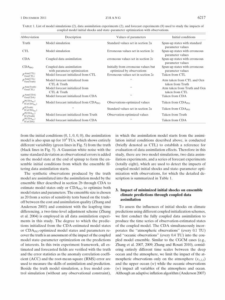
TABLE 1. List of model simulations (2), data assimilation experiments (2), and forecast experiments (8) used to study the impacts of

coupled model initial shocks and state–parameter optimization with observations.

Abbreviation Description Values of parameters Initial conditions

Truth Model simulation Standard values set in section 2a Spun-up states with standard

parameter values

CTL Model simulation Erroneous values set in section 2c Spun-up states with erroneous

parameter values

CDA Coupled data assimilation erroneous values set in section 2c Spun-up states with erroneous

parameter values

CDAPO Coupled data assimilation

with parameter optimization

Initially from erroneous values but

optimized by observations

Spun-up states with erroneous

parameter values

FAtm(CTL)Ocn(CTL) Model forecast initialized from CTL Erroneous values set in section 2c Taken from CTL

FAtm(CTL)Ocn(Truth) Model forecast initialized from

CTL & Truth

’’ Atm taken from CTL and Ocn

taken from Truth

FAtm(Truth)Ocn(CTL) Model forecast initialized from

CTL & Truth

’’ Atm taken from Truth and Ocn

taken from CTL

FAtm(CDA)Ocn(CDA) Model forecast initialized from CDA ’’ Taken from CDA

FP(CDAPO)

ICs(CDAPO) Model forecast initialized from CDAPO Observations-optimized values Taken from CDAPO

FP(Truth)ICs(CDAPO) ’’ Standard values set in section 2a Taken from CDAPO

FP(CDAPO)

ICs(Truth) Model forecast initialized from Truth Observation-optimized values Taken from Truth

FP(CDAPO)

ICs(CDA) Model forecast initialized from CDA ’’ Taken from CDA


is available for a sophisticated system, for this simple

system, a best-tuned inflation coefficient of 1.12 is ap-

plied to the prior ensemble of the atmosphere and upper-

ocean variables. The CDA reconstructs the truth vari-

ability of the atmosphere and ocean mostly as shown in

Fig. 5, quantified by the high ACC values (0.8 for the

atmosphere and 0.89 for the ocean) and the significantly

reduced RMS errors (by 47% for the atmosphere’’ and by

63% for the ocean) compared to the free model control

without initialization (CTL) (Table 2). The results here

show that different from a filter with an unbiased assimi-

lation model where the assimilation error can be expected

smaller than the observational error by tuning the filtering

inflation, a filter with a biased coupled model in which

some component with large time-scale variability lacks

observations may not well converge by tuning the filtering

inflation. Section 4 will show that under this circumstance,

while the model states are constrained by observations,

properly optimizing the model parameters using observa-

tions is particularly important to make the filter convergent.

Next, we use the notation F with a subscript that rep-

resents the oceanic initial conditions and a superscript for

atmospheric initial conditions, so that FAtm(CDA)Ocn(CDA) stands for

the forecast experiment in which both the atmosphere

and the ocean of the coupled model are initialized from

the CDA-estimated states. Beside FAtm(CDA)Ocn(CDA) another

two forecast experiments FAtm(Truth)Ocn(CTL) and F

Atm(CTL)Ocn(Truth)

also are used for assessing the impact of minimized initial

shocks of CDA on climate predictions. In FAtm(Truth)Ocn(CTL)

(FAtm(CTL)Ocn(Truth)), the model ensemble is initialized from the

perfect atmosphere (ocean) taken from the truth combined

with the CTL oceanic (atmospheric) ensemble as shown

by the dashed-green lines in Fig. 5. Another forecast ex-

periment in which both the atmosphere and the ocean are

initialized from the CTL ensemble coupled states, called

FAtm(CTL)Ocn(CTL) , is used as a reference to establish the value of

the initialization for the coupled model prediction. The

detailed description of all the forecast experiments per-

formed in this study can be found in Table 1. For each

experiment, we launch 50 forecasts, each with a lead time

of 500 TUs. The initial conditions are taken every 500 TUs

apart over the period of 104 to 4 3 104 TUs. Figures 6

and 7 show some examples of the forecasted atmo-

spheric (Fig. 6) and oceanic (Fig. 7) states produced by

FAtm(CDA)Ocn(CDA) (left columns) and F

Atm(CTL)Ocn(Truth) (right columns),

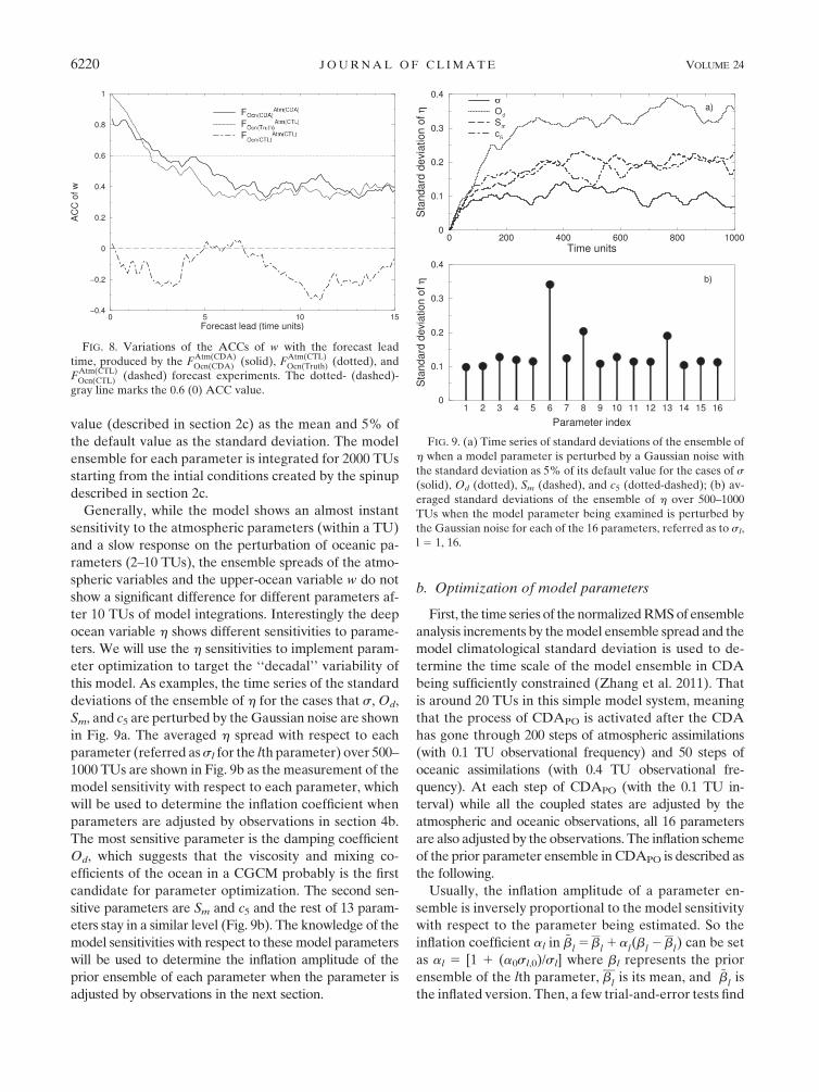
while Fig. 8 shows the variation of the forecasted ACCs of

the upper-ocean variable w with the forecast lead times.

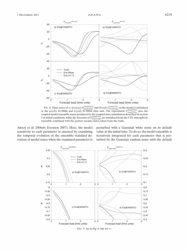
Generally, compared to the coherent initial conditions

of FAtm(CDA)Ocn(CDA) (Figs. 6a,c and Figs. 7a,c), an inconsistency

exists between x2 and w in the initial conditions of

FAtm(Truth)Ocn(CTL) and F

Atm(CTL)Ocn(Truth) (only the F

Atm(CTL)Ocn(Truth) case is shown).

While the imbalance caused by the inconsistency pro-

duces a zig-zag variation for the w (Figs. 7b,d), due to the

strong internal variability of the atmosphere, the compu-

tational variability of the atmosphere caused by the im-

balance is formed very rapidly (Figs. 6b,d). Specifically,

in this simple system, the computational oscillations of x2

caused by the imbalance between the atmospheric and

oceanic initial conditions increase the ‘‘noises’’ of the ‘‘at-

mospheric’’ forcings to w. These increased errors on the

‘‘atmospheric’’ fluxes to the ‘‘ocean’’ produce a larger de-

creasing rate of the forecast ACC of w with the forecast

lead times in FAtm(CTL)Ocn(Truth) than in F

Atm(CDA)Ocn(CDA) (Fig. 8), resulting

lesser forecast skills of FAtm(CTL)Ocn(Truth) after 1.5-TU forecasts even

though it starts from the perfect oceanic initial condi-

tions.

It is worth mentioning that due to the marginal impact

of the upper ocean on the deep ocean in this simple

model (as shown in Fig. 3a), the initial shocks induced by

the imbalance between x2 and w in the initial conditions

of FAtm(Truth)Ocn(CTL) and F

Atm(CTL)Ocn(Truth) do not explicitly influence

on the forecast skills of the deep ocean adversely.

4. Impact of the coupled model state–parameteroptimization on climate predictions

The results of section 3 show that when a filter is ap-

plied to a biased coupled model in which some compo-

nent with large time-scale variability lacks observations,

it is difficult to make the filter convergent through tuning

the filtering inflation. In this section, the author will show

that under such a circumstance, properly optimizing model

parameters using observations is an effective approach

to enhance the accuracy of state estimation and improve

model predictions.

a. Model sensitivities on parameters

The sensitivity study of a model on parameters is an

important step to understand the role of each parameter

in the model and implement parameter estimation (e.g.,

Tong and Xue 2008a,b). In particular, the sensitivity of

a model to a parameter is a key to determine the inflation

of the prior ensemble of the parameter, which is an in-

dispensable part of ensemble-based parameter estima-

tion (e.g., Annan and Hargreaves 2004; Annan et al. 2005;

TABLE 2. The RMS errors and ACCs of the atmospheric and

oceanic variables in CDA and CDAPO as well as a free model

control ensemble simulation (CTL).

Expt

Rms ACC

Atm Ocn Atm Ocn

x1 x2 x3 w h x1 x2 x3 w h

CTL 152 242 313 3.1 0.38 — — — — —

CDA 52 130 170 1.2 0.10 0.84 0.78 0.77 0.87 0.91

CDAPO 0.44 1.3 1.5 0.16 0.03 1 1 1 1 1


Aksoy et al. 2006ab; Evensen 2007). Here, the model

sensitivity to each parameter is assessed by examining

the temporal evolution of the ensemble standard de-

viation of model states when the examined parameter is

perturbed with a Gaussian white noise on its default

value at the initial time. To do so, the model ensemble is

iteratively integrated for each parameter that is per-

turbed by the Gaussian random noise with the default

FIG. 6. Time series of x2 in (a),(c) FAtm(CDA)Ocn(CDA) and (b),(d) F

Atm(CTL)Ocn(Truth) as the model is initialized

at the (a),(b) 10 000th and (c),(d) 30 000th time unit. The experiment FAtm(CDA)Ocn(CDA) uses the

coupled model ensemble states produced by the coupled data assimilation described in section

3 as initial conditions, while the forecasts of FAtm(CTL)Ocn(Truth) are initialized from the CTL atmospheric

ensemble combined with the perfect oceanic states taken from the truth.

FIG. 7. As in Fig. 6, but for w.


value (described in section 2c) as the mean and 5% of

the default value as the standard deviation. The model

ensemble for each parameter is integrated for 2000 TUs

starting from the intial conditions created by the spinup

described in section 2c.

Generally, while the model shows an almost instant

sensitivity to the atmospheric parameters (within a TU)

and a slow response on the perturbation of oceanic pa-

rameters (2–10 TUs), the ensemble spreads of the atmo-

spheric variables and the upper-ocean variable w do not

show a significant difference for different parameters af-

ter 10 TUs of model integrations. Interestingly the deep

ocean variable h shows different sensitivities to parame-

ters. We will use the h sensitivities to implement param-

eter optimization to target the ‘‘decadal’’ variability of

this model. As examples, the time series of the standard

deviations of the ensemble of h for the cases that s, Od,

Sm, and c5 are perturbed by the Gaussian noise are shown

in Fig. 9a. The averaged h spread with respect to each

parameter (referred as sl for the lth parameter) over 500–

1000 TUs are shown in Fig. 9b as the measurement of the

model sensitivity with respect to each parameter, which

will be used to determine the inflation coefficient when

parameters are adjusted by observations in section 4b.

The most sensitive parameter is the damping coefficient

Od, which suggests that the viscosity and mixing co-

efficients of the ocean in a CGCM probably is the first

candidate for parameter optimization. The second sen-

sitive parameters are Sm and c5 and the rest of 13 param-

eters stay in a similar level (Fig. 9b). The knowledge of the

model sensitivities with respect to these model parameters

will be used to determine the inflation amplitude of the

prior ensemble of each parameter when the parameter is

adjusted by observations in the next section.

b. Optimization of model parameters

First, the time series of the normalized RMS of ensemble

analysis increments by the model ensemble spread and the

model climatological standard deviation is used to de-

termine the time scale of the model ensemble in CDA

being sufficiently constrained (Zhang et al. 2011). That

is around 20 TUs in this simple model system, meaning

that the process of CDAPO is activated after the CDA

has gone through 200 steps of atmospheric assimilations

(with 0.1 TU observational frequency) and 50 steps of

oceanic assimilations (with 0.4 TU observational fre-

quency). At each step of CDAPO (with the 0.1 TU in-

terval) while all the coupled states are adjusted by the

atmospheric and oceanic observations, all 16 parameters

are also adjusted by the observations. The inflation scheme

of the prior parameter ensemble in CDAPO is described as

the following.

Usually, the inflation amplitude of a parameter en-

semble is inversely proportional to the model sensitivity

with respect to the parameter being estimated. So the

inflation coefficient al in ~bl5 b

l1 a

l(b

l2 b

l) can be set

as al 5 [1 1 (a0sl,0)/sl] where bl represents the prior

ensemble of the lth parameter, bl is its mean, and ~bl is

the inflated version. Then, a few trial-and-error tests find

FIG. 8. Variations of the ACCs of w with the forecast lead

time, produced by the FAtm(CDA)Ocn(CDA) (solid), F

Atm(CTL)Ocn(Truth) (dotted), and

FAtm(CTL)Ocn(CTL) (dashed) forecast experiments. The dotted- (dashed)-

gray line marks the 0.6 (0) ACC value.

FIG. 9. (a) Time series of standard deviations of the ensemble of

h when a model parameter is perturbed by a Gaussian noise with

the standard deviation as 5% of its default value for the cases of s

(solid), Od (dotted), Sm (dashed), and c5 (dotted-dashed); (b) av-

eraged standard deviations of the ensemble of h over 500–1000

TUs when the model parameter being examined is perturbed by

the Gaussian noise for each of the 16 parameters, referred as to sl,

l 5 1, 16.


a0 5 1023. This means that the prior ensemble of a pa-

rameter is enlarged to 1023/sl times of its initially

guessed standard deviation sl,0 if the prior ensemble

spread is smaller than this amount.

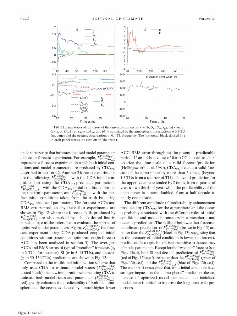
The errors of the ensemble means of typical atmo-

spheric and oceanic state variables and all parameters

varying with the times of CDAPO are shown in Figs. 10

and 11, respectively, in which the parameters are grou-

ped according to their relative amplitudes of varying in

different panels in Fig. 11. Figure 10 clearly shows that

the CDAPO process adjusts both model states and pa-

rameters efficiently and constrains model uncertainties

more dramatically than the CDA, evidenced by the di-

minishingly smaller oceanic errors and atmospheric er-

rors compared to the CDA errors (reduced by 85%, see

also Table 2).

Because of the compensative effect among all pa-

rameters and state variables in an ensemble filter (Yang

and DelSole 2009), the optimization of parameters—

expressed as a multivariate regression process of obser-

vational increments as formulated as Eq. (3)— does not

however necessarily mean that each parameter converges

to its truth. In fact, the solution of parameter optimiza-

tion is a synthetic product of available observations,

model sensitivities with respect to parameters as well as

other model bias sources except for erroneously set pa-

rameters. In this case, although only the erroneous model

parameters serve as the only source of model bias, due to

different availability of atmospheric and oceanic observa-

tions and the dependence of the parameter optimization

on the deep ocean sensitivity, the subset of parameters

has a different behavior in the optimization. For example,

four atmospheric parameters, s, b (Fig. 11a), k (Fig. 11b),

and c1 (Fig. 11c) converge to their truth values very quickly

while not all 12 oceanic parameters do so. It turns out that

while the initial errors of eight oceanic parameters Om,

Sm, Spd (Fig. 11a), G (Fig. 11b), c3, c4, c6 (Fig. 11c), and g

(Fig. 11d) are greatly reduced through the optimization,

the errors of the other four oceanic parameters Ss, Od,

c2, and c5 are not significantly reduced, some of them

being even increased (Ss, for instance).

c. Impact of optimized model parameterson climate predictions

In this section, to assess the role of optimizing model

parameters using observations for long time-scale pre-

dictions, four new forecast experiments (see Table 1) are

conducted. In particular, to represent the different com-

bination of model initial conditions and parameters, here

an F with a subscript that indicates the initial conditions

FIG. 10. Time series of the errors of the ensemble means of (a) x1, (b) w, and (c) h produced

by CDAPO (red) in which the parameter correction is activated at the 20th TU and traditional

CDA (green). The free model ensemble CTL for which the assimilation model starts from the

same ensemble initial conditions as CDA and CDAPO but without any data constraint is also

plotted in blue in each panel as a reference. The pair of the numbers in the parenthesis for each

line is the corresponding root-mean-square error (RMSE) and ACC verified with the truth.

Fig(s). 10 live 4/C


and a superscript that indicates the used model parameters

denotes a forecast experiment. For example, FP(CDAPO)

ICs(CDAPO)

represents a forecast experiment in which both initial con-

ditions and model parameters are produced by CDAPO

described in section 4.2. Another 3 forecast experiments

are the following: FP(CDAPO)

ICs(CDA) —with the CDA initial con-

ditions but using the CDAPO-produced parameters,

FP(Truth)ICs(CDAPO)—with the CDAPO initial conditions but us-

ing the truth parameter, and FICs(Truth)P(CDAPO)—with the per-

fect initial conditions taken from the truth but using

CDAPO-produced parameters. The forecast ACCs and

RMS errors produced by these four experiments are

shown in Fig. 12 where the forecast skills produced by

FAtm(CDA)Ocn(CDA) are also marked by a black-dotted line in

panels a, b, c as the reference to evaluate the impact of

optimized model parameters. Again, FAtm(CDA)Ocn(CDA) is a fore-

cast experiment using CDA-produced coupled initial

conditions without parameter optimization (its forecast

ACC has been analyzed in section 3). The averaged

ACCs and RMS errors of typical ‘‘weather’’ forecasts (x1

in 2 TUs, for instance), SI (w in 5–15 TUs), and decadal

(h in 50–150 TUs) predictions are shown in Fig. 13.

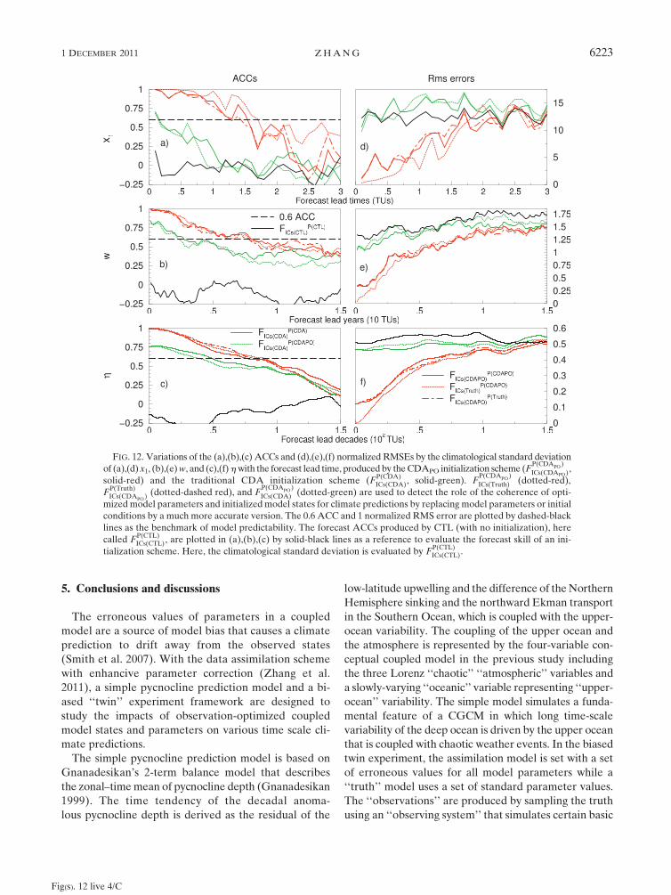
Compared to the traditional initialization scheme that

only uses CDA to estimate model states (FAtm(CDA)Ocn(CDA)

dotted-black), the new initialization scheme using CDA to

estimate both model states and parameters (FICs(CDAPO)P(CDAPO) ,

red) greatly enhances the predictability of both the atmo-

sphere and the ocean, evidenced by a much higher–lower

ACC–RMS error throughout the potential predictable

period. If an ad hoc value of 0.6 ACC is used to char-

acterize the time scale of a valid forecast/prediction

(Hollingsworth et al. 1980), CDAPO extends a valid fore-

cast of the atmosphere by more than 5 times, (beyond

1.5 TUs from a quarter of TU). The valid prediction for

the upper ocean is extended by 2 times, from a quarter of

year to two thirds of year, while the predictability of the

deep ocean is almost doubled, from a half decade to

nearly one decade.

The different amplitude of predictability enhancement

produced by CDAPO for the atmosphere and the ocean

is probably associated with the different roles of initial

conditions and model parameters in atmospheric and

oceanic predictions. The skills of both weather forecasts

and climate predictions of FP(CDAPO)

ICs(CDA) (brown in Fig. 13) are

better than the FAtm(CDA)Ocn(CDA) (black in Fig. 13), suggesting that

as the accuracy of initial conditions is lower, the forecast/

prediction of a coupled model is not sensitive to the accuracy

of model parameters. Except for the ‘‘weather’’ forecast (see

Figs. 13a,d), both SI and decadal predictions of FP(CDAPO)

ICs(CDA)

(red of Figs. 13b,c,e,f) are better than the FP(CDAPO)

ICs(Truth) (green of

Figs. 13b,c,e,f) and the FP(Truth)ICs(CDAPO) (blue of Figs. 13b,c,e,f).

These comparisons address that, while initial conditions have

stronger impacts on the ‘‘atmospheric’’ prediction, the co-

herence of optimized model parameters and initialized

model states is critical to improve the long time-scale pre-

dictions.

FIG. 11. Time series of the errors of the ensemble means of (a) s, b, Om, Sm, Spd, (b) k and G,

(c) c1, c2, Od, Ss, c3, c4, c5 and c6, and (d) g optimized by the atmospheric observations at 0.1-TU

frequency and the oceanic observations at 0.4-TU frequency. The horizontal black-dashed line

in each panel marks the zero error (the truth).

Fig(s). 11 live 4/C


5. Conclusions and discussions

The erroneous values of parameters in a coupled

model are a source of model bias that causes a climate

prediction to drift away from the observed states

(Smith et al. 2007). With the data assimilation scheme

with enhancive parameter correction (Zhang et al.

2011), a simple pycnocline prediction model and a bi-

ased ‘‘twin’’ experiment framework are designed to

study the impacts of observation-optimized coupled

model states and parameters on various time scale cli-

mate predictions.

The simple pycnocline prediction model is based on

Gnanadesikan’s 2-term balance model that describes

the zonal–time mean of pycnocline depth (Gnanadesikan

1999). The time tendency of the decadal anoma-

lous pycnocline depth is derived as the residual of the

low-latitude upwelling and the difference of the Northern

Hemisphere sinking and the northward Ekman transport

in the Southern Ocean, which is coupled with the upper-

ocean variability. The coupling of the upper ocean and

the atmosphere is represented by the four-variable con-

ceptual coupled model in the previous study including

the three Lorenz ‘‘chaotic’’ ‘‘atmospheric’’ variables and

a slowly-varying ‘‘oceanic’’ variable representing ‘‘upper-

ocean’’ variability. The simple model simulates a funda-

mental feature of a CGCM in which long time-scale

variability of the deep ocean is driven by the upper ocean

that is coupled with chaotic weather events. In the biased

twin experiment, the assimilation model is set with a set

of erroneous values for all model parameters while a

‘‘truth’’ model uses a set of standard parameter values.

The ‘‘observations’’ are produced by sampling the truth

using an ‘‘observing system’’ that simulates certain basic

FIG. 12. Variations of the (a),(b),(c) ACCs and (d),(e),(f) normalized RMSEs by the climatological standard deviation

of (a),(d) x1, (b),(e) w, and (c),(f) h with the forecast lead time, produced by the CDAPO initialization scheme (FP(CDAPO)

ICs(CDAPO),

solid-red) and the traditional CDA initialization scheme (FP(CDA)ICs(CDA), solid-green). F

P(CDAPO)

ICs(Truth) (dotted-red),

FP(Truth)ICs(CDAPO) (dotted-dashed red), and F

P(CDAPO)

ICs(CDA) (dotted-green) are used to detect the role of the coherence of opti-

mized model parameters and initialized model states for climate predictions by replacing model parameters or initial

conditions by a much more accurate version. The 0.6 ACC and 1 normalized RMS error are plotted by dashed-black

lines as the benchmark of model predictability. The forecast ACCs produced by CTL (with no initialization), here

called FP(CTL)ICs(CTL), are plotted in (a),(b),(c) by solid-black lines as a reference to evaluate the forecast skill of an ini-

tialization scheme. Here, the climatological standard deviation is evaluated by FP(CTL)ICs(CTL).

Fig(s). 12 live 4/C


features of the atmospheric and oceanic measurements

in the real climate observing system. Then the synthetic

atmospheric and oceanic observations are assimilated into

the assimilation model to recover the truth, producing

initial conditions and observation-optimized model pa-

rameters from which the model is initialized to predict

the truth. The degree to which the predictions initialized

from the estimated coupled model states from the tradi-

tional coupled data assimilation (e.g., Zhang et al. 2007)

or the observation-optimized model states and param-

eters recover the truth is used to assess the impacts of the

traditional coupled data assimilation and the coupled

model state–parameter optimization scheme on the cli-

mate predictions of interests.

While the coupled model initialization through coupled

data assimilation in which all coupled model components

are coherently adjusted by observations minimizes the

initial coupling shocks that reduce the forecast errors on

seasonal-interannual time scales, the new initialization

scheme that uses observations to optimize both coupled

model states and parameters greatly enhances the pre-

dictability of the model on all time scales. For example,

while the valid forecasts of the atmosphere are extended

by more than 5 times, the predictability of the deep

ocean is almost doubled. In addition, while the im-

proved initial conditions from the new scheme have

stronger impacts on the atmospheric forecasts, the co-

herence of optimized model parameters and initialized

model states is critical to improve the long time-scale

predictions.

Although the coupled state–parameter optimization

using observations has shown great promise with the sim-

ple pycnocline prediction model, serious challenges exist

when it is applied to CGCMs to improve decadal pre-

dictions. First, in this simple model study, the errors of

model parameters are the only source of model bias. In

a CGCM, the misfittings from complex physical pro-

cesses and dynamical core introduce multiple sources

for model bias. The performance of the coupled state–

parameter optimization scheme at the presence of mul-

tiple model biases needs to be examined further. Second,

successful parameter optimization requires the good rep-

resentation of an observing system and relies on the ac-

curacy of estimated states. We may allow a parameter that

traditionally takes a globally uniform value to vary geo-

graphically to reflect the geographical dependence of

model sensitivity and observational availability. Given

numerous parameters in a CGCM and the importance

of model sensitivity knowledge in parameter optimi-

zation (Tong and Xue 2008a), a thorough sensitivity

study of a CGCM with respect to its all parameters is

a key but challenging first step. We may first start with

FIG. 13. The time-averaged (left) ACCs and (right) RMS errors of (a),(d) x1 in the forecast

lead time of 2 TUs, (b),(e) w in the forecast lead time of 5–15 TUs, and (c),(f) h in the forecast

lead time of 50–150 TUs, produced by the forecast experiment 1--FP(CDAPO)

ICs(CDAPO) (red),

2--FP(CDAPO)

ICs(Truth) (green), 3--FP(Truth)ICs(CDAPO) (blue), 4--F

P(CDAPO)

ICs(CDA) (black), and 5–FAtm(CDA)Ocn(CDA) (brown).

Fig(s). 13 live 4/C


a few important (sensitive) parameters, which would

have to be defined based on the modeler’s knowledge

about physical parameterizations. Theoretically, in-

cluding parameters into assimilation control variables

increases the freedom of an assimilation system so that

the misfittings of climate modeling can be more efficiently

constrained by observations thus reducing model biases.

Once certain parameters that are sensitive for the pro-

cesses of decadal variability [e.g. the North Atlantic

overturning (Delworth et al. 1993) and the Pacific Rossby

waves associated with the Pacific decadal oscillations

(Schneider and Cornuelle 2005)] are identified and op-

timized, the improvement of decadal climate predictions

through optimizing parameters of the CGCM holds

promises.

Acknowledgments. Special thanks go to Tony Rosati,

Tom Delworth at GFDL, and Prof. Z. Liu at Wis-

consin University for their persistent support and en-

couragement on this research. Thanks go to Drs. Rym

Msadek and You-Soon Chang for their helpful com-

ments on a preliminary version of this paper. This

research is supported by the NSF project Grant

0968383.

REFERENCES

Aksoy, A., F. Zhang, and J. W. Nielsen-Gammon, 2006a: En-

semble-based simultaneous state and parameter estimation

with MM5. Geophys. Res. Lett., 33, L12801, doi:10.1029/

2006GL026186.

——, ——, and ——, 2006b: Ensemble-based simultaneous state

and parameter estimation in a two-dimensional sea-breeze

model. Mon. Wea. Rev., 134, 2951–2970.

Anderson, J. L., 2001: An ensemble adjustment Kalman filter for

data assimilation. Mon. Wea. Rev., 129, 2884–2903.

——, 2003: A local least squares framework for ensemble filtering.

Mon. Wea. Rev., 131, 634–642.

——, 2007: An adaptive covariance inflation error correction al-

gorithm for ensemble filters. Tellus, 59A, 210–224.

Annan, J. D., and J. C. Hargreaves, 2004: Efficient parameter

estimation for a highly chaotic system. Tellus, 56A, 520–

526.

——, ——, N. R. Edwards, and R. Marsh, 2005: Parameter es-

timation in an intermediate complexity earth system model

using an ensemble Kalman filter. Ocean Modell., 8, 135–

154.

Asselin, R., 1972: Frequency filter for time integrations. Mon. Wea.

Rev., 100, 487–490.

Cherupin, D., J. A. Carton, and D. Dee, 2005: Forecast model bias

correction in ocean data assimilation. Mon. Wea. Rev., 133,

1328–1342.

Collins, W. D., M. L. Blackman, G. B. Bonan, J. J. Hack, T. B.

Henderson, J. T. Kiehl, W. G. Large, and D. S. Mckenna, 2006:

The Community Climate System Model version 3 (CCSM3).

J. Climate, 19, 2122–2143.

Dee, D. P., 2005: Bias and data assimilation. Quart. J. Roy. Meteor.

Soc., 131, 3323–3343.

——, and A. M. D. Silva, 1998: Data assimilation in the pres-

ence of forecast bias. Quart. J. Roy. Meteor. Soc., 124, 269–

295.

DelSole, T., and X. Yang, 2010: State and parameter estima-

tion in stochastic dynamical models. Physica D, 239, 1781–

1788.

Delworth, T. L., S. Manabe, and R. J. Stouffer, 1993: Interdecadal

variations of the thermohaline circulation in a coupled ocean-

atmosphere model. J. Climate, 6, 1993–2011.

——, and Coauthors, 2006: GFDL’s CM2 global coupled climate

models. Part I: Formulation and simulation characteristics.

J. Climate, 19, 643–674.

Evensen, G., 1994: Sequential data assimilation with a nonlinear

quasi-geostrophic model using Monte Carlo methods to

forecast error statistics. J. Geophys. Res., 99, 10 143–10 162.

——, 2007: Data Assimilation: The Ensemble Kalman Filter.

Springer Press, 279 pp.

Gnanadesikan, A., 1999: A simple predictive model for the

structure of the oceanic pycnocline. Science, 283, 2077–

2079.

Hamill, T. M., J. S. Whitaker, and C. Snyder, 2001: Distance-

dependent filtering of background error covariance esti-

mates in an ensemble Kalman filter. Mon. Wea. Rev., 129,

2776–2790.

Hansen, J., and C. Penland, 2007: On stochastic parameter esti-

mation using data assimilation. Physica D, 230, 88–89.

Hollingsworth, A., K. Arpe, M. Tiedtke, M. Capaldo, and H. Savijarvi,

1980: The performance of a medium-range forecast model

in winter—Impact of physical parameterizations. Mon. Wea.

Rev., 108, 1736–1773.

Keenlyside, N. S., M. Latif, J. Jungclaus, L. Kornblueh, and

E. Roeckner, 2008: Advancing decadal-scale climate pre-

diction in the North Atlantic sector. Nature, 453, 84–88.

Kondrashov, D., C. Sun, and M. Ghil, 2008: Data assimilation for

a coupled ocean-atmosphere model. Part II: Parameter esti-

mation. Mon. Wea. Rev., 136, 5062–5076.

Lorenz, E. N., 1963: Deterministic non-periodic flow. J. Atmos.

Sci., 20, 130–141.

Robert, A., 1969: The integration of a spectral model of the at-

mosphere by the implicit method. Proc. WMO/IUGG Symp.

on NWP, Tokyo, Japan, Japan Meteorological Society, 19–

24.

Schneider, N., and B. D. Cornuelle, 2005: The forcing of the Pacific

decadal oscillation. J. Climate, 18, 4355–4373.

Smith, D. M., S. Cusack, A. W. Colman, C. K. Folland, G. R.

Harris, and J. M. Murphy, 2007: Improved surface tempera-

ture prediction for the coming decade from a global climate

model. Science, 317, 796–799.

Tong, M., and M. Xue, 2008a: Simultaneous estimation of micro-

physical parameters and atmospheric state with simulated

radar data and ensemble square root Kalman filter. Part I:

Sensitivity analysis and parameter identifiability. Mon. Wea.

Rev., 136, 1630–1648.

——, and ——, 2008b: Simultaneous estimation of microphysical

parameters and atmospheric state with simulated radar

data and ensemble square root Kalman filter. Part II: Pa-

rameter estimation experiments. Mon. Wea. Rev., 136,

1649–1668.

Yang, X., and T. DelSole, 2009: Using the ensemble Kalman Filter

to estimate multiplicative model parameters. Tellus, 61A,

601–609.

Zhang, S., 2011: Impact of observation-optimized model parameters

on decadal predictions: Simulation with a simple pycnocline


prediction model. Geophys. Res. Lett., 38, L02702, doi:10.1029/

2010GL046133.

——, and J. L. Anderson, 2003: Impact of spatially and temporally

varying estimates of error covariance on assimilation in

a simple atmospheric model. Tellus, 55A, 126–147.

——, and A. Rosati, 2010: An inflated ensemble filter for ocean

data assimilation with a biased coupled GCM. Mon. Wea.

Rev., 138, 3905–3931.

——, J. L. Anderson, A. Rosati, M. J. Harrison, S. P. Khare, and

A. Wittenberg, 2004: Multiple time level adjustment for data

assimilation. Tellus, 56A, 2–15.

——, M. J. Harrison, A. Rosati, and A. T. Wittenberg, 2007: System

design and evaluation of coupled ensemble data assimilation for

global oceanic climate studies. Mon. Wea. Rev., 135, 3541–3564.

——, ——, and M. J. Harrison, 2009: Detection of multidecadal

oceanic variability by ocean data assimilation in the context of

a ‘‘perfect’’ coupled model. J. Geophys. Res., 114, C12018,

doi:10.1029/2008JC005261.

——, Z. Liu, A. Rosati, and T. Delworth, 2011: A study of en-

hancive parameter correction with coupled data assimilation

for climate estimation and prediction using a simple coupled

model. Tellus A, in press.


a study of impacts of coupled model initial shocks and ... · a study of impacts of coupled model...

Documents