a solo-based automated quality control algorithm for ... · a solo-based automated quality control...

A Solo-Based Automated Quality Control Algorithm for Airborne TailDoppler Radar Data

MICHAEL M. BELL

University of Hawai’i at M~anoa, Honolulu, Hawaii

WEN-CHAU LEE, CORY A. WOLFF, AND HUAQING CAI

National Center for Atmospheric Research,* Boulder, Colorado

(Manuscript received 15 October 2012, in final form 5 April 2013)

ABSTRACT

An automated quality control preprocessing algorithm for removing nonweather radar echoes in airborne

Doppler radar data has been developed. This algorithm can significantly reduce the time and experience level

required for interactive radar data editing prior to dual-Doppler wind synthesis or data assimilation. The

algorithm uses the editing functions in the Solo software package developed by the National Center for

Atmospheric Research to remove noise, Earth-surface, sidelobe, second-trip, and other artifacts. The char-

acteristics of these nonweather radar returns, the algorithm to identify and remove them, and the impacts of

applying different threshold levels on wind retrievals are presented. Verification was performed by com-

parison with published Electra Doppler Radar (ELDORA) datasets that were interactively edited by dif-

ferent experienced radar meteorologists. Four cases consisting primarily of convective echoes from the

Verification of the Origins of Rotation in Tornadoes Experiment (VORTEX), Bow Echo and Mesoscale

Convective Vortex Experiment (BAMEX), Hurricane Rainband and Intensity Change Experiment

(RAINEX), and The Observing SystemResearch and Predictability Experiment (THORPEX) Pacific Asian

Regional Campaign (T-PARC)/Tropical Cyclone Structure-2008 (TCS08) field experiments were used to test

the algorithm using three threshold levels for data removal. The algorithm removes 80%, 90%, or 95% of the

nonweather returns and retains 95%, 90%, or 85% of the weather returns on average at the low-, medium-,

and high-threshold levels. Increasing the threshold level removes more nonweather echoes at the expense of

also removing more weather echoes. The low threshold is recommended when weather retention is the

highest priority, and the high threshold is recommendedwhen nonweather removal is the highest priority. The

medium threshold is a good compromise between these two priorities and is recommended for general use.

Dual-Doppler wind retrievals using the automatically edited data compare well to retrievals from in-

teractively edited data.

1. Introduction

Airborne Doppler radars are currently some of the

best tools for deducing mesoscale three-dimensional

wind and precipitation structures within weather systems

at long range from an operations center. They have been

the primary tools for deducing the internal structure of

mesoscale weather phenomena such as bow echoes,

convective boundary layers, fronts, hurricanes, meso-

scale convective systems, tornadoes, and winter storms

[Lee et al. (2003) and references therein]. Raw airborne

Doppler data contain both weather and nonweather

echoes that require editing and quality control (QC) prior

to wind synthesis, but interactive QC has been a hin-

drance for researchers because of the time and training

required to properly identify nonweather radar echoes.

To date, this interactive editing process has not been

systematically documented. The purpose of the current

study is to (i) document the characteristics of nonweather

echoes in airborne Doppler radar, (ii) design an algo-

rithm to preprocess airborne Doppler QC automatically

to reduce both the time and necessary experience level

*The National Center for Atmospheric Research is sponsored

by the National Science Foundation.

Corresponding author address: Michael M. Bell, Dept. of Me-

teorology, University of Hawai’i at M~anoa, 2525 Correa Rd.,

Honolulu, HI 96822.

E-mail: [email protected]

NOVEMBER 2013 BELL ET AL . 2509

DOI: 10.1175/JAMC-D-12-0283.1

� 2013 American Meteorological Society

mailto:[email protected]

for data users, and (iii) validate the algorithm and exam-

ine its impact on derived products such as dual-Doppler

synthesis and radar data assimilation.

The Electra Doppler Radar (ELDORA)/Analyese

Stereoscopic par Impulsions Aeroporte (ASTRAIA)

system (Hildebrand et al. 1996), operated by theNational

Center for Atmospheric Research (NCAR), has the best

spatial resolution of any currently operating airborne

Doppler precipitation radar. ELDORA has two sepa-

rate antennas that can scan rapidly at ;24 revolutions

per minute, with a complete revolution of each radar

available every 3 s. The two antennas are oriented ;168fore and aft of the cross-fuselage axis (i.e., aircraft

heading) so that the radar beams overlap in space as

the aircraft moves forward. The ELDORA scanning

strategy allows for dual-Doppler retrievals of the three-

dimensional wind with 300–500-m spatial resolution,

providing a tremendous advantage that can only be

realized after this prodigious amount of data is quality

controlled.

The QC process consists of airborne navigation and

pointing angle corrections (Testud et al. 1995; Bosart

et al. 2002), followed by interactive data editing. The

interactive QC process of airborne Doppler radar data

using the NCAR Solo software requires a significant

amount of time even for experienced radar meteorolo-

gists, with rough estimates of up to 30min to edit a single

radar scan. As a result, interactive editing of 10min

worth of ELDORA radar data takes up to 240 h by this

estimate.With the algorithmdescribed herein, the editing

time for the 10min of ELDORA data can be decreased

significantly, from several weeks down to a few days or

hours, depending on the intended use of the radar data.

A variety of algorithms to identify and remove non-

weather radar echoes have been developed for ground-

based radars (Steiner and Smith 2002; Lakshmanan et al.

2007), but many of the components from ground-based

QC are not directly applicable to airborne radar data

(Bousquet and Smull 2003). For example, the surface

echo characteristics are quite different with airborne

Doppler radars than with ground-based radars. Airborne

tail radars scan in an axis approximately perpendicular

to the aircraft track, such that the radar scans trace out a

helix in space.A ‘‘cluttermap’’ can bemade for a ground-

based radar that indicates where stationary targets such

as trees, terrain, or man-made structures are present, but

a static clutter map is not possible for a moving platform.

Bousquet and Smull (2003) alternatively used a digital

terrain map to identify echoes from Earth’s surface in

their semiautomated QC algorithm for airborne radar

data. However, QC algorithms based on spatial patterns

and numerical characteristics of the radar data may be

generally applicable. Bousquet and Smull (2003) also

used a running-mean outlier detection algorithm based

on Bargen and Brown (1980), similar to that used in

ground-based applications, with further QC performed

interactively.

Gamache (2005) developed an algorithm for the au-

tomatic QC of data collected in hurricanes by the Na-

tional Oceanic and Atmospheric Association (NOAA)

Tail Doppler Radar (TDR). The algorithm uses rule-

based procedures similar to the algorithm presented

herein, but the procedures and technical implementa-

tion are different. The Gamache (2005) algorithm was

developed for the specific context of hurricane re-

connaissance, with a primary focus of providing real-

time dual-Doppler winds for the National Hurricane

Center and National Centers for Environmental Pre-

diction. Hurricane-specific features, such as the appro-

ximate circular symmetry of the wind field and fixed

operational flight patterns, can be exploited to improve

the QC process. Because ELDORA is a research radar

operated within the context of National Science Foun-

dation (NSF)-funded field experiments, both the ob-

served phenomena and the data collection strategy

change from project to project, requiring a more gen-

eral algorithm. One of the recorded data fields from

ELDORA that is an important part of the current QC

algorithm is the normalized coherent power (NCP), but

this field is not currently computed by theNOAATDRor

used in the Gamache (2005) algorithm.

Velocity aliasing can be of concern for the NOAA

TDRwhen using a single pulse repetition frequency with

a relatively small Nyquist velocity (often 12.9m s21).

Although the technical implementation is different, both

NOAA TDR and ELDORA have the ability to use a

dual-pulse repetition frequency scheme to extend the

Nyquist velocity to 60–80ms21 and essentially eliminate

aliasing (Hildebrand et al. 1996; Jorgensen et al. 2000).

The algorithm presented here does not include dealiasing

as explicitly as in Gamache (2005), but can be included if

required (Bargen and Brown 1980).

The algorithm development was guided by two main

design goals: (i) to be general enough to handle a wide

variety of situations but specific enough to significantly

reduce QC time and (ii) to be implemented within the

context of the Solo interactive data editor. The first

design goal makes the algorithm generally applicable,

but sacrifices advantages that could be obtained from

tuning for a specific weather regime. The current al-

gorithm was therefore designed within the context of

convective weather given the preponderance of con-

vective cases in the ELDORA data archive. The trade-

off is practical, but limits its applicability to a subset of

the ELDORA archive andmay be suboptimal for some

weather regimes.

2510 JOURNAL OF APPL IED METEOROLOGY AND CL IMATOLOGY VOLUME 52

The second design goal was to develop the QC pre-

processing algorithm using the Solo interactive data

editor (Oye et al. 1995). In contrast to a stand-alone,

operationalQC application like that inGamache (2005),

a Solo script–based procedure can be easily distributed

to existing Solo users without requiring any additional

software. The batch-editing scripts can also be used by

researchers as a starting point for further interactive

editing within the Solo environment. The trade-off with

the second design goal is that algorithm components

were limited to those available as existing Solo editing

operations. A set of tunable parameters was developed

with Solo components to meet different editing criteria

using ‘‘low,’’ ‘‘medium,’’ and ‘‘high’’ thresholds for data

removal. It will be shown that increasing the threshold

level removes more nonweather echoes at the expense of

removing more weather echoes also. Although good re-

sults are obtained with the current algorithm, one result

of this study is that rule-based procedures with tunable

parameters such as those available within Solo may ulti-

mately be suboptimal for weather discrimination. The

current work helps pave the way for a more complex al-

gorithm with multidimensional classification metrics.

All radar QC algorithms suffer from a lack of an

established ‘‘ground truth’’ for validation. Nonweather

echo characteristics are highly variable, and it is difficult

to design a synthetic verification dataset that captures this

variability for different radars and weather conditions.

Determining whether a given radar volume consists of a

weather or nonweather echo ultimately depends on a

radar meteorologist’s subjective appraisal of the scene

and experience level. Although some volumes are easily

classifiable, others are more ambiguous and may be

classified differently by different researchers. The ap-

proach taken in this study was to validate the QC algo-

rithm using datasets edited by different researchers from

multiple field projects. The selected datasets are taken

from published papers by experienced ELDORA users,

and provide a reasonable baseline for validation and

statistical verification of the algorithm using dichotomous

classification metrics (Stanski et al. 1989; Woodcock

1976). The verification approach contains some potential

biases, but it is expected that differences between data-

sets and researchers’ editing styles would remove any

large systematic biases in the verification statistics.

The desired product from a quality controlled airborne

Doppler dataset is typically a wind retrieval or improved

initial conditions for a numerical simulation. Although

there are many studies that address dual-Doppler and

radar data assimilation techniques, considerably less at-

tention has been paid to the impacts of radarQCon these

techniques. The impacts of the different thresholds of data

removal on a dual-Doppler retrieval from a developing

tropical cyclone were examined, confirming the results of

a previous study that wind retrievals using the QC algo-

rithm were robust compared to their interactively edited

counterparts (Schmitz 2010). Impacts of the QC algo-

rithm on radar data assimilation (Zhang et al. 2012) will

also be summarized here. These results suggest that the

algorithm proves useful for preparing airborne radar

data for assimilation into numerical weather prediction

models, for real-time dual-Doppler during a research

flight to aid a mission scientist in making decisions

about where to next send the aircraft (Houze et al.

2006), or for initial QC prior to further interactive ed-

iting of detailed case studies in postanalysis mode.

The outline of this paper is as follows. Descriptions of

the nonweather echoes in airborne radar data and clas-

sification procedures are presented in section 2. The

validation and statistical verification of the QC algorithm

are presented in section 3. Impacts on dual-Doppler

retrievals and radar data assimilation are presented in

section 4. A summary and concluding remarks are pre-

sented in section 5. Technical details of the Solo software

and the automated QC algorithm are described in the

appendixes for interested readers.

2. Classification of echoes in airborne tail Dopplerradar data

a. Characteristics of nonweather echoes

A returned radar signal is quantified by the zero, first,

and second radar moments that correspond to the

reflectivity (hereinafter the units dBZ are used to in-

dicate reflectivity), Doppler velocity, and spectral width

(SW), respectively. The dBZ is directly proportional to

the returned power and the strength of the Doppler

velocity signal. The Doppler velocity is a statistical es-

timate frommultiple pulses that can be affected by noise

in the received signal and radar electronics. The SW

indicates the variance of the Doppler velocity within the

radar pulse volume because of noise, turbulence, wind

shear, differential fall speed, and antenna motion. A less

commonly used radar parameter is the normalized co-

herent power (NCP), which is defined by the ratio of the

power in the first moment (also called coherent power) to

the total returned power. NCP quantifies the relative

power used to calculate the Doppler velocity with the

total power used to calculate dBZ, and is approximately

inversely proportional to SW.

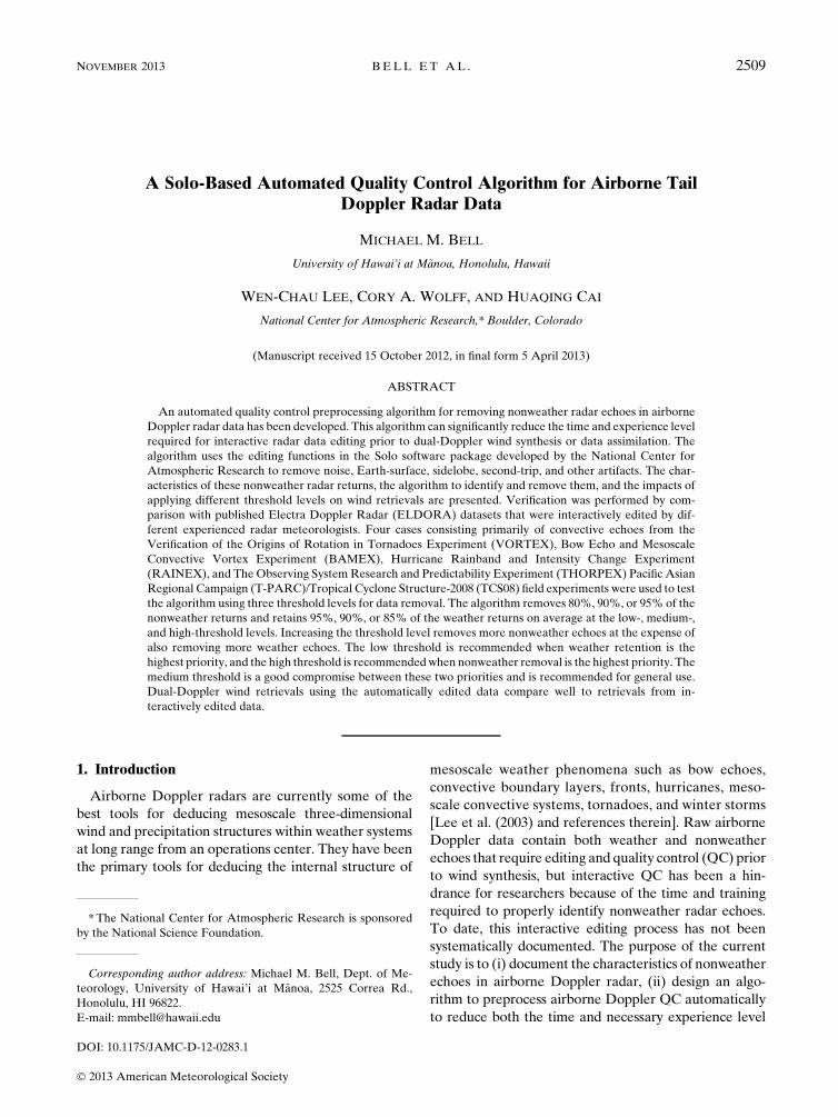
An unedited ELDORA radar sweep from The Ob-

serving System Research and Predictability Experi-

ment (THORPEX) Pacific Asian Regional Campaign

(T-PARC)/Tropical Cyclone Structure-2008 (TCS08)

field campaign that illustrates these radar parameters is

shown in Fig. 1. The radar image is from the aft-pointing


antenna at 2351:31 UTC on 14 September 2008. The

Naval Research Laboratory’s P-3 aircraft position is at

the center of each panel, and a large convective echo and

anvil are evident to the right of the aircraft. The four

panels in Fig. 1 show dBZ, Doppler velocity, SW, and

NCP. Five main types of data can be identified in Fig. 1:

weather, noise, surface, radar sidelobes, and second-trip

echoes. Gray shading indicates values off the color scale,

and the locations of the nonweather echoes have been

highlighted. Noise regions are characterized by low dBZ

with a logarithmic range dependence, and random

Doppler velocities. The SW and NCP fields distinguish

predominately signal and noise regions with a rela-

tively sharp demarcation.

The tail Doppler scanning strategy yields a prominent

surface echo with a high dBZ, near-zeroDoppler velocity

over land (or the corresponding ocean surface velocity),

and a low SW. The surface echo is a thin, multigate echo

directly beneath the aircraft, but it expands in width at

longer ranges and becomes difficult to distinguish from

the strong convective echoes at low altitude to the right

of the aircraft. For ELDORA, there is also some cross

contamination from the multiple frequencies used in the

complex ‘‘chip’’ pulse (Hildebrand et al. 1996). The close

proximity of these frequencies results in a broadening of

the surface echo in range comparable with that of the

single-frequency NOAA TDR.1 Reflected atmospheric

echoes appear beneath the ground.

FIG. 1. Example of radar echoes from predepression Hagupit at 2351:30 UTC 14 Sep 2008

during T-PARC/TCS08. Shown is the (a) dBZ (increment 5 4 dBZ), (b) Doppler velocity

(increment 5 2m s21), (c) SW (increment 5 1.5m s21), and (d) NCP (increment 5 0.05).

Nonweather echoes are labeled in (a).

1Multiple-frequency contamination can be considered a ‘‘range

sidelobe’’ similar to contamination by sidelobe energy found off

the main beam axis. The range sidelobe can sometimes also be

found on the edge of strong weather echoes.


Although partial beamfilling by surface echo would

occur even with a ‘‘perfect’’ Gaussian radar beam, we

define ‘‘sidelobe echoes’’ as those resulting from distinct

peaks in the power in the tail of the radar beam by an-

tenna diffraction. The sidelobe surface reflection mani-

fests itself as a ring of moderate dBZ and low velocity

around the aircraft, with flared echoes near the base of

the ring that appear to emanate from the surface. The

diameter of the sidelobe surface ring is dependent on the

altitude of the aircraft, with larger rings as the aircraft flies

higher. The strongest sidelobe echoes are located near

the surface at approximately 208–308 from nadir, and are

characterized by a high NCP, moderate dBZ, and mod-

erate SW. Reflectivity decreases in the ‘‘flared’’ portion

of the echo farther from the surface, but the velocity

signal is nearly constant throughout the echo. Sidelobe

echoes occur primarily in clear-air regions, but the

boundary between the sidelobe echo and the weather

echo is often very subtle.

A ‘‘second trip’’ echo is a radar echo from a previous

pulse that returns from longer range and is combined

with the processing of the current pulse at shorter range.

The second-trip echo is evident as a large reflectivity

wedge on the left side of Fig. 1a, and is due to a combi-

nation of returns from both the surface (below flight

level) and convective weather (above the flight level) at

long range. On the right side of the aircraft, the stronger,

first-trip convective echo dominates the returned power

and no second-trip echo is evident. The second-trip

echo appears as a spike in the reflectivity field with a ran-

dom Doppler velocity, a moderate NCP, and a high SW.

Modern signal-processing techniques have been iden-

tified to separate multitrip echoes, such as phase coding

(Sachidananda and Zrnic 1999; Frush et al. 2002) that

may be implemented in future radar upgrades.

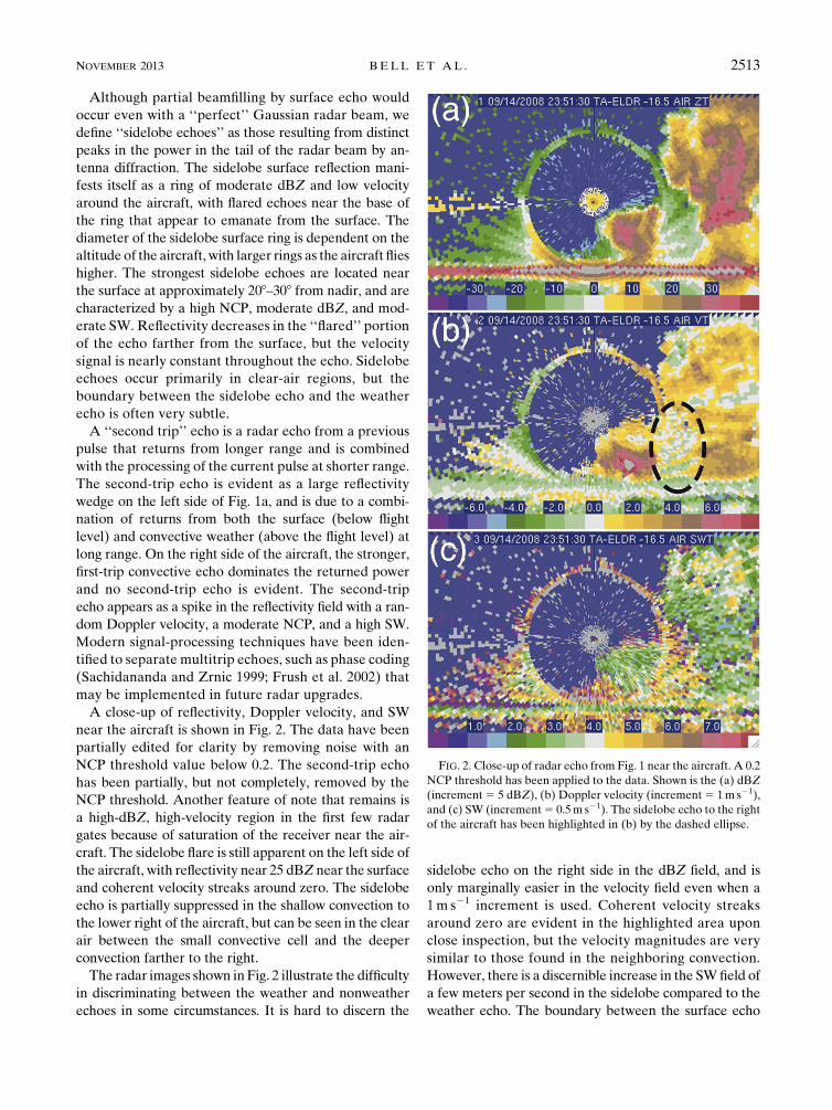
A close-up of reflectivity, Doppler velocity, and SW

near the aircraft is shown in Fig. 2. The data have been

partially edited for clarity by removing noise with an

NCP threshold value below 0.2. The second-trip echo

has been partially, but not completely, removed by the

NCP threshold. Another feature of note that remains is

a high-dBZ, high-velocity region in the first few radar

gates because of saturation of the receiver near the air-

craft. The sidelobe flare is still apparent on the left side of

the aircraft, with reflectivity near 25 dBZ near the surface

and coherent velocity streaks around zero. The sidelobe

echo is partially suppressed in the shallow convection to

the lower right of the aircraft, but can be seen in the clear

air between the small convective cell and the deeper

convection farther to the right.

The radar images shown in Fig. 2 illustrate the difficulty

in discriminating between the weather and nonweather

echoes in some circumstances. It is hard to discern the

sidelobe echo on the right side in the dBZ field, and is

only marginally easier in the velocity field even when a

1m s21 increment is used. Coherent velocity streaks

around zero are evident in the highlighted area upon

close inspection, but the velocity magnitudes are very

similar to those found in the neighboring convection.

However, there is a discernible increase in the SWfield of

a few meters per second in the sidelobe compared to the

weather echo. The boundary between the surface echo

FIG. 2. Close-up of radar echo from Fig. 1 near the aircraft. A 0.2

NCP threshold has been applied to the data. Shown is the (a) dBZ

(increment5 5 dBZ), (b) Doppler velocity (increment5 1m s21),

and (c) SW (increment5 0.5m s21). The sidelobe echo to the right

of the aircraft has been highlighted in (b) by the dashed ellipse.


and deep convection is also difficult to discern in this

example. The lack of any ground-truth validation com-

pounds the difficulty in definitively classifying these am-

biguous echoes.

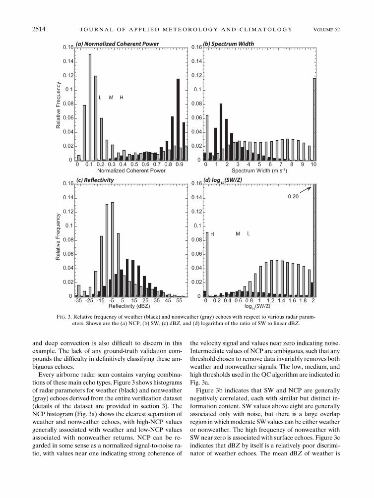
Every airborne radar scan contains varying combina-

tions of thesemain echo types. Figure 3 shows histograms

of radar parameters for weather (black) and nonweather

(gray) echoes derived from the entire verification dataset

(details of the dataset are provided in section 3). The

NCP histogram (Fig. 3a) shows the clearest separation of

weather and nonweather echoes, with high-NCP values

generally associated with weather and low-NCP values

associated with nonweather returns. NCP can be re-

garded in some sense as a normalized signal-to-noise ra-

tio, with values near one indicating strong coherence of

the velocity signal and values near zero indicating noise.

Intermediate values of NCP are ambiguous, such that any

threshold chosen to remove data invariably removes both

weather and nonweather signals. The low, medium, and

high thresholds used in the QC algorithm are indicated in

Fig. 3a.

Figure 3b indicates that SW and NCP are generally

negatively correlated, each with similar but distinct in-

formation content. SW values above eight are generally

associated only with noise, but there is a large overlap

region in whichmoderate SWvalues can be eitherweather

or nonweather. The high frequency of nonweather with

SW near zero is associated with surface echoes. Figure 3c

indicates that dBZ by itself is a relatively poor discrimi-

nator of weather echoes. The mean dBZ of weather is

FIG. 3. Relative frequency of weather (black) and nonweather (gray) echoes with respect to various radar param-

eters. Shown are the (a) NCP, (b) SW, (c) dBZ, and (d) logarithm of the ratio of SW to linear dBZ.


higher than that of nonweather, but there is considerable

overlap in the distributions. Although SW and dBZ are

not great discriminators by themselves, the combination

of these parameters contains more information (Fig. 3d).

In general, high SW associated with high dBZ would be

more indicative of turbulent convection or wind shear,

whereas high SW associated with low dBZ would be

more indicative of noise. The ratio of SW to reflectivity

in the QC algorithm is discussed further in the following

section.

b. Automatic quality control algorithm

There have been relatively few automated QC algo-

rithms developed for airborne weather radar, but one

area that has received a thorough treatment is the re-

moval of surface echo. For flat continental or oceanic

returns, the primary radar gates affected by the surface

can be identified by the intersection of the main lobe of

the radar beamwith the surface (Lee et al. 1994a; Testud

et al. 1995). The issue of surface removal in complex

terrain was addressed by Georgis et al. (2000) and

Bousquet and Smull (2003) through the use of a digital

terrain map. Complex terrain removal is not currently

part of the Solo software, highlighting one limitation of

the existing QC framework used in this study.2

The above studies focused on the removal of surface

echoes within the main lobe (defined by the half-power

beamwidth), but the strong backscatter from the surface

can contaminate a radar volume with only a small inter-

section of the ‘‘tail’’ of the beam and bias the Doppler

velocity toward zero. One advancement in the current

QC algorithm is the use of a variable ‘‘effective’’ beam-

width in the Testud et al. (1995) algorithm to remove data

with partial beamfilling by surface echo. The use of a

wider beamwidth removes partial surface echoes left

behind in the original form of the algorithm.

While the removal of all radar range gates, even those

potentially affected by the surface, may be desired for

some applications, excessive removal of near-surface

echoes can be detrimental for dual-Doppler synthesis.

Overestimating the amount of surface echo contami-

nation can significantly affect the magnitude and even

the sign of the retrieved vertical velocity because of the

strong dependence on the measured low-level diver-

gence. The variability of the partial surface echo depends

on the strength of the near-surface weather echo and

beam broadening with range, but without additional

signal processing of the Doppler velocity time series it

is impossible to quantitatively determine how much a

near-surface radar volume has been affected by the

surface.

A key advancement of the current study is the exten-

sion of automatic QC procedures beyond the removal of

surface echo. The basic editing procedure performed by

the automatic QC algorithm consists of nine steps, which

are shown in Table 1 and described in more detail in

appendix B for interested readers. Some of the relevant

details of the algorithm are summarized here.

The Solo scripts used to execute the algorithm steps

can be configured with user-defined threshold values

that offer a compromise between the amount of weather

and nonweather data removed. Three basic threshold

levels were defined as low, medium, and high, with the

corresponding script parameters shown in Table 2. The

use of a general, procedural approach necessitates

the use of broad characteristics for data removal rather

than specific feature identification. The three threshold

levels in the QC algorithm for NCP, SW, and dBZ are

indicated in Figs. 3a and 3d. Removing data with a low

NCP is very effective at eliminating noise, as evidenced

by the histogram.At the low threshold almost no weather

echo is removed, but increasing the threshold to remove

more undesirable nonweather echoes also consequently

removes more-desirable weather echoes.

The ratio of SW to dBZ was found to be a good iden-

tifier of sidelobe echoes, and Fig. 3d shows the logarithm

of the ratio of SW to dBZ converted to its linear value

(mm26m23) for dBZ values less than zero. A SW/dBZ

ratio near zero is ambiguous, but increasing values of the

ratio are associated with higher probabilities of non-

weather. It is noted that the high threshold uses a 5-dBZ

value, which increases the relative frequency of weather

slightly compared to Fig. 3d. While most ground-based

algorithms include SW and dBZ information, the SW/

dBZ parameter is a novel combination to the authors’

knowledge. The ratio is not explicitly calculated in Solo,

but a combination of SW and dBZ that mimics this pa-

rameter is included in the algorithm.

It is also noted that the order in which the Solo com-

ponents are executed plays an important role in the al-

gorithm, such that successively finer discriminations are

TABLE 1. Description of editing steps in the QC algorithm.

(i) Back up original reflectivity and velocity fields

(ii) Remove data with an NCP value below a specified threshold

(iii) Remove noisy data at edges of radar range

(iv) Remove the direct surface returns

(v) Remove data with high SW and low dBZ

(vi) Despeckle the data

(vii) Defreckle the data

(viii) Second despeckle pass

(ix) Synchronize the reflectivity and velocity fields

2 This functionality has been implemented in a stand-alone ver-

sion of the QC algorithm.


made after coarser data removal. For example, the

‘‘despeckling’’ and ‘‘defreckling’’ algorithms described

in appendix B were found to be effective at removing

isolated data, noise, and second-trip echoes after the

bulk of nonweather echo was removed.

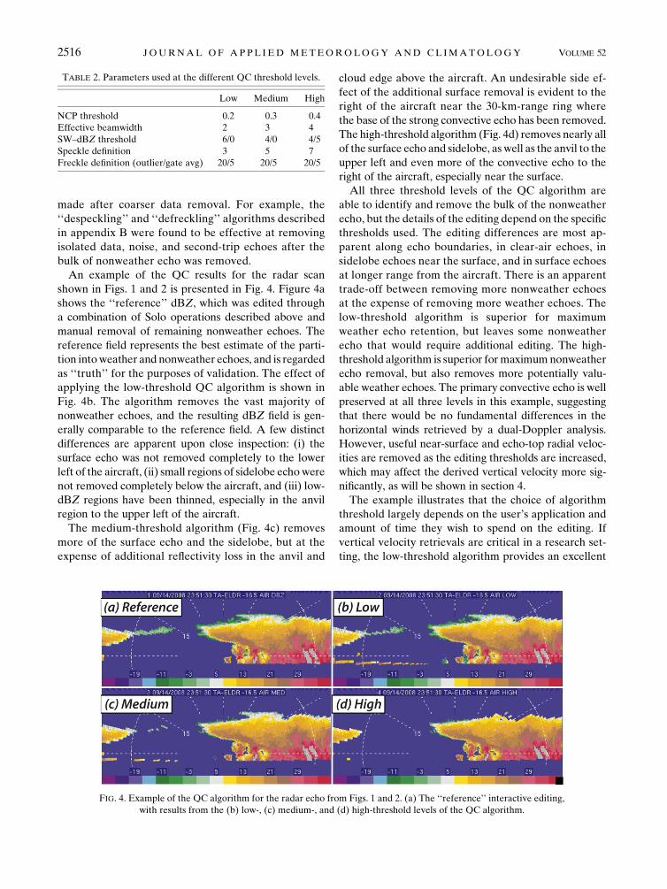
An example of the QC results for the radar scan

shown in Figs. 1 and 2 is presented in Fig. 4. Figure 4a

shows the ‘‘reference’’ dBZ, which was edited through

a combination of Solo operations described above and

manual removal of remaining nonweather echoes. The

reference field represents the best estimate of the parti-

tion intoweather and nonweather echoes, and is regarded

as ‘‘truth’’ for the purposes of validation. The effect of

applying the low-threshold QC algorithm is shown in

Fig. 4b. The algorithm removes the vast majority of

nonweather echoes, and the resulting dBZ field is gen-

erally comparable to the reference field. A few distinct

differences are apparent upon close inspection: (i) the

surface echo was not removed completely to the lower

left of the aircraft, (ii) small regions of sidelobe echowere

not removed completely below the aircraft, and (iii) low-

dBZ regions have been thinned, especially in the anvil

region to the upper left of the aircraft.

The medium-threshold algorithm (Fig. 4c) removes

more of the surface echo and the sidelobe, but at the

expense of additional reflectivity loss in the anvil and

cloud edge above the aircraft. An undesirable side ef-

fect of the additional surface removal is evident to the

right of the aircraft near the 30-km-range ring where

the base of the strong convective echo has been removed.

The high-threshold algorithm (Fig. 4d) removes nearly all

of the surface echo and sidelobe, aswell as the anvil to the

upper left and even more of the convective echo to the

right of the aircraft, especially near the surface.

All three threshold levels of the QC algorithm are

able to identify and remove the bulk of the nonweather

echo, but the details of the editing depend on the specific

thresholds used. The editing differences are most ap-

parent along echo boundaries, in clear-air echoes, in

sidelobe echoes near the surface, and in surface echoes

at longer range from the aircraft. There is an apparent

trade-off between removing more nonweather echoes

at the expense of removing more weather echoes. The

low-threshold algorithm is superior for maximum

weather echo retention, but leaves some nonweather

echo that would require additional editing. The high-

threshold algorithm is superior formaximumnonweather

echo removal, but also removes more potentially valu-

able weather echoes. The primary convective echo is well

preserved at all three levels in this example, suggesting

that there would be no fundamental differences in the

horizontal winds retrieved by a dual-Doppler analysis.

However, useful near-surface and echo-top radial veloc-

ities are removed as the editing thresholds are increased,

which may affect the derived vertical velocity more sig-

nificantly, as will be shown in section 4.

The example illustrates that the choice of algorithm

threshold largely depends on the user’s application and

amount of time they wish to spend on the editing. If

vertical velocity retrievals are critical in a research set-

ting, the low-threshold algorithm provides an excellent

TABLE 2. Parameters used at the different QC threshold levels.

Low Medium High

NCP threshold 0.2 0.3 0.4

Effective beamwidth 2 3 4

SW–dBZ threshold 6/0 4/0 4/5

Speckle definition 3 5 7

Freckle definition (outlier/gate avg) 20/5 20/5 20/5

FIG. 4. Example of the QC algorithm for the radar echo from Figs. 1 and 2. (a) The ‘‘reference’’ interactive editing,

with results from the (b) low-, (c) medium-, and (d) high-threshold levels of the QC algorithm.


starting point for subsequent interactive editing. For data

assimilation applications, the loss of some good weather

echoes may have a minimal impact compared to the in-

sertion of radar artifacts into the model, especially if the

data are subsequently ‘‘super obbed’’ after quality con-

trol (Zhang et al. 2012). The trade-offs presented for

the current example are generally applicable for most

ELDORA radar cases, but the details depend on the

meteorological situation and aircraft sampling strategy.

3. Algorithm verification

a. Verification statistics

Verification of the QC algorithm was conducted using

multiple radar datasets. The test dataset was chosen from

four field programs in which ELDORA was involved

(Fig. 5). Each case represents a different mesoscale re-

gime so that theQC algorithm could be tested in a variety

of meteorological situations. The verification data are

1344 radar scans that were interactively edited by expe-

rienced radar meteorologists and used in case studies

published in the refereed literature. The sample dataset

contains 48min of data and over 60 million radar gates,

which provides a reasonable sample for calculating sta-

tistics. It is recognized that data editing is subjective and

editing styles among these experienced radar meteorol-

ogists may vary, which could produce a bias in the sta-

tistical results presented. However, averaging over the

variety of weather conditions and editing styles is ex-

pected to reduce the bias from any one case. Table 3

provides information about each of the cases used for the

verification including the times of each of the flight legs.

The field experiments are the Verification of the Origins

of Rotation in Tornadoes Experiment (VORTEX), Bow

Echo and Mesoscale Convective Vortex Experiment

(BAMEX), Hurricane Rainband and Intensity Change

Experiment (RAINEX), and T-PARC/TCS08. The

VORTEX (Wakimoto et al. 1998) and BAMEX

(Wakimoto et al. 2004) cases represent different types of

midlatitude continental convection. The RAINEX

(Houze et al. 2006) and T-PARC/TCS08 (Bell and

Montgomery 2009) cases represent tropical oceanic sys-

tems in different stages of development.

Measures of the skill of the QC algorithm can be de-

rived using 2 3 2 contingency tables where hits, misses,

and false positives can be collected for each case. The

edited data are treated as dichotomous values where each

gate in the sample is defined as either ‘‘positive’’ weather

or ‘‘negative’’ nonweather. A radar gate where both the

QC algorithm and verification dataset have identified a

weather echo is considered a correct positive result. A

gate where both have identified a nonweather echo is

considered a correct negative result. Correct positive and

negative results are considered hits. Radar gates falsely

identified as weather echoes by the QC algorithm are

considered false positives. Radar gates falsely identified

as nonweather echoes are considered misses.

A typical sweep of data from ELDORA contains

muchmore nonweather echo than weather (cf. Fig. 1a to

Fig. 4a). The algorithm skill scores would be dominated

by data that are obviously not weather without a base-

line edit of the raw data. To get meaningful statistics,

some very basic QC techniques were applied to the raw

data before the fields were run through the full QC al-

gorithm. Data with NCP below 0.2, radar echoes at and

below the surface identified with a 1.88 beamwidth, and

echoes above 25-km altitude were removed prior to the

verification. The baseline edited data allow for the

evaluation of the algorithm on data that are more diffi-

cult to classify as weather or nonweather.

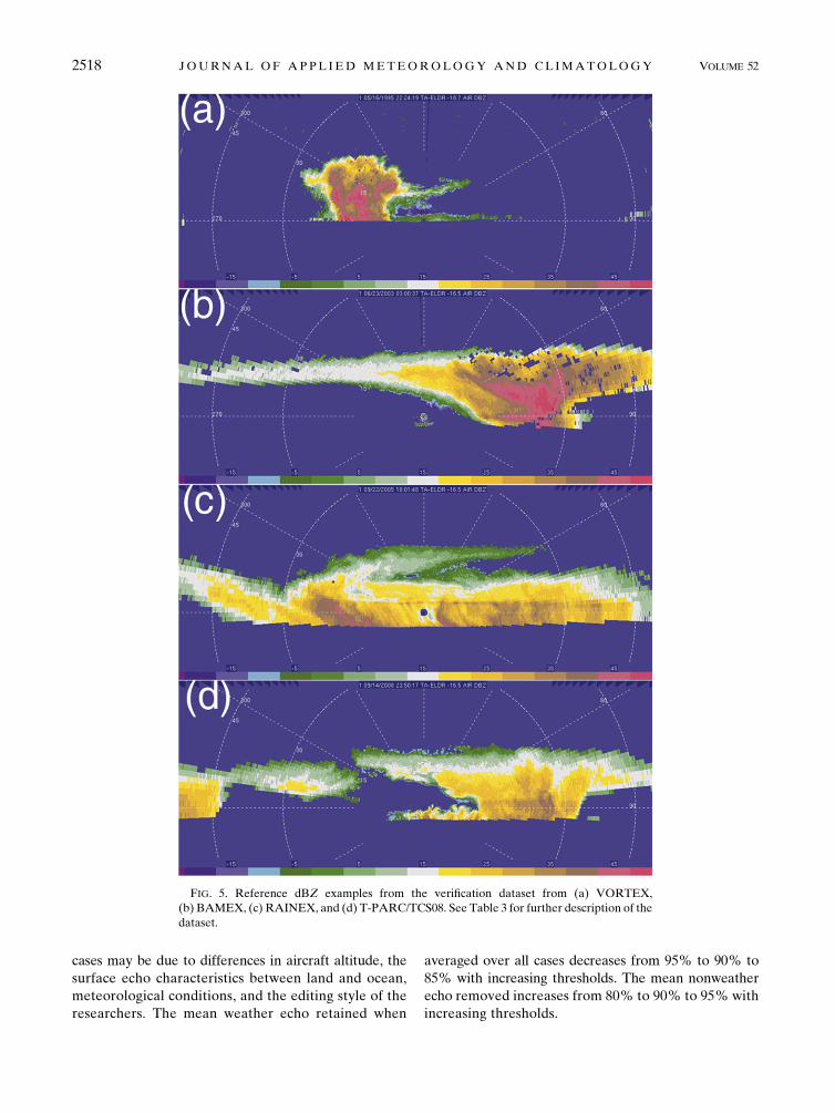
Figure 6 shows a receiver operating characteristic

(ROC; Joliffe and Stephenson 2003) plot that displays the

relationship between correctly identified events (hits)

versus falsely identified events (false positives) for the

low, medium, and high thresholds. Anything to the upper

left of the 1:1 line across the ROC plot in Fig. 6a is con-

sidered to have positive skill. A perfect algorithm with

retention of all weather data and the removal of all

nonweather data would give results in the top-left corner

of the chart. The three data points for each test case

represent the average amount of data retained after ap-

plication of the method using the three different thresh-

olds. The rightmost points on each curve denote the low

threshold and the leftmost points denote the high

threshold. Thresholds in the algorithm could be tuned by

the user to yield different levels of editing between the

high and low points illustrated here. The curves are near

the top-left corner for the current algorithm, but trace

counterclockwise as the QC thresholds are increased.

The two primary goals of the algorithm—to retain all

weather and remove all nonweather—cannot be met

simultaneously and involve trade-offs as the thresholds

are increased.

The ROC curve is the best for RAINEX (green line),

with over 95% of the weather retained and 88% of

nonweather removed at all thresholds on average. The

RAINEX case was located in the outer eyewall of Hur-

ricane Rita in 2005 and the data contain large regions of

stratiform and convective weather echoes. The other

tropical case from T-PARC/TCS08 (black line) per-

formed the second best, with almost all nonweather data

removed at the high threshold. The continental cases

from VORTEX (blue line) and BAMEX (red line) still

verify well, but with less skill than the oceanic cases. The

differences in skill between the oceanic and continental


cases may be due to differences in aircraft altitude, the

surface echo characteristics between land and ocean,

meteorological conditions, and the editing style of the

researchers. The mean weather echo retained when

averaged over all cases decreases from 95% to 90% to

85% with increasing thresholds. The mean nonweather

echo removed increases from 80% to 90% to 95% with

increasing thresholds.

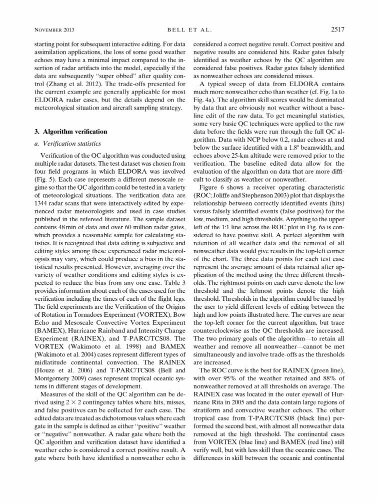
FIG. 5. Reference dBZ examples from the verification dataset from (a) VORTEX,

(b) BAMEX, (c) RAINEX, and (d) T-PARC/TCS08. See Table 3 for further description of the

dataset.


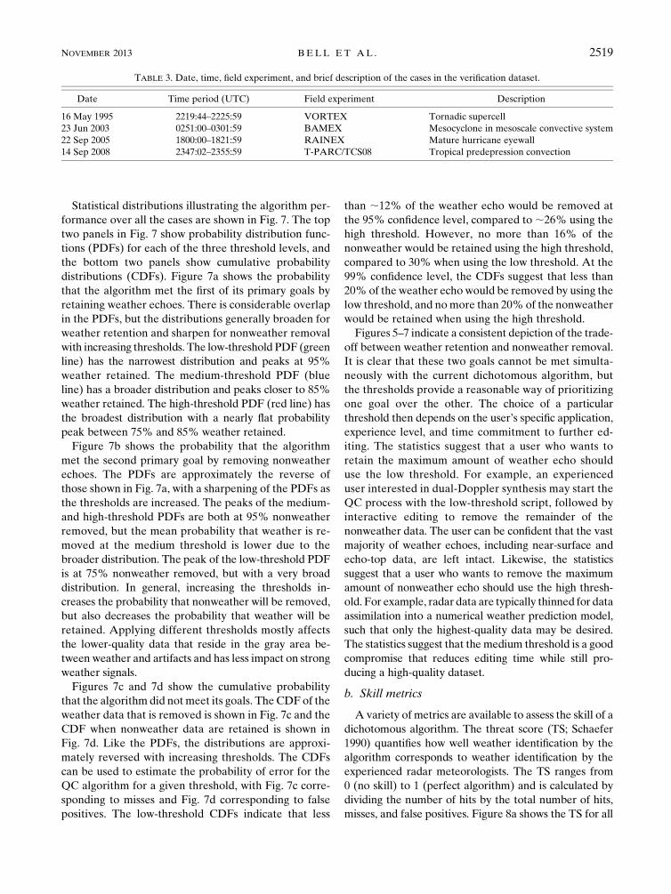
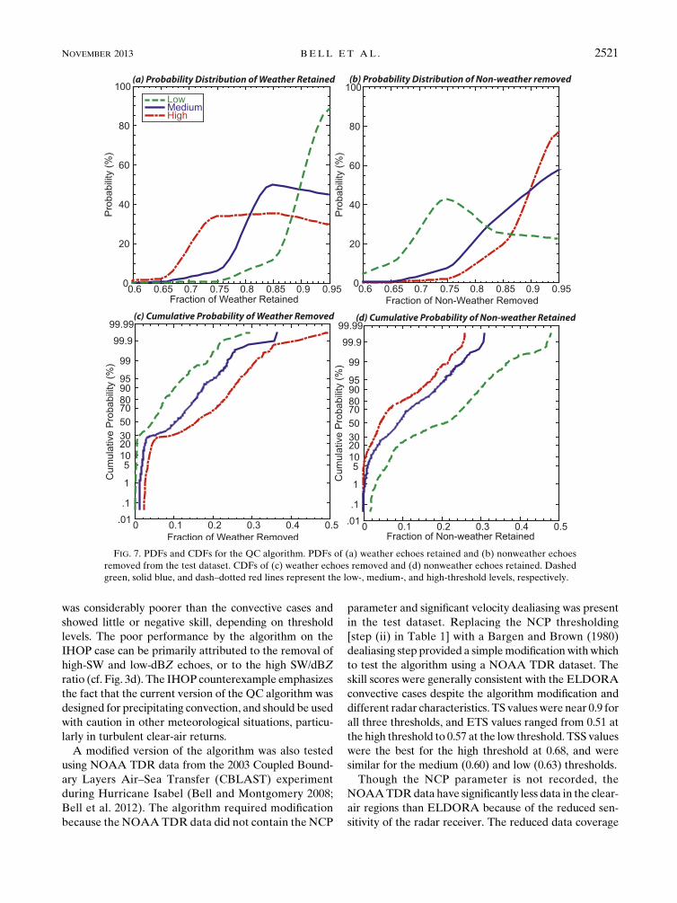
Statistical distributions illustrating the algorithm per-

formance over all the cases are shown in Fig. 7. The top

two panels in Fig. 7 show probability distribution func-

tions (PDFs) for each of the three threshold levels, and

the bottom two panels show cumulative probability

distributions (CDFs). Figure 7a shows the probability

that the algorithm met the first of its primary goals by

retaining weather echoes. There is considerable overlap

in the PDFs, but the distributions generally broaden for

weather retention and sharpen for nonweather removal

with increasing thresholds. The low-threshold PDF (green

line) has the narrowest distribution and peaks at 95%

weather retained. The medium-threshold PDF (blue

line) has a broader distribution and peaks closer to 85%

weather retained. The high-threshold PDF (red line) has

the broadest distribution with a nearly flat probability

peak between 75% and 85% weather retained.

Figure 7b shows the probability that the algorithm

met the second primary goal by removing nonweather

echoes. The PDFs are approximately the reverse of

those shown in Fig. 7a, with a sharpening of the PDFs as

the thresholds are increased. The peaks of the medium-

and high-threshold PDFs are both at 95% nonweather

removed, but the mean probability that weather is re-

moved at the medium threshold is lower due to the

broader distribution. The peak of the low-threshold PDF

is at 75% nonweather removed, but with a very broad

distribution. In general, increasing the thresholds in-

creases the probability that nonweather will be removed,

but also decreases the probability that weather will be

retained. Applying different thresholds mostly affects

the lower-quality data that reside in the gray area be-

tween weather and artifacts and has less impact on strong

weather signals.

Figures 7c and 7d show the cumulative probability

that the algorithm did notmeet its goals. The CDF of the

weather data that is removed is shown in Fig. 7c and the

CDF when nonweather data are retained is shown in

Fig. 7d. Like the PDFs, the distributions are approxi-

mately reversed with increasing thresholds. The CDFs

can be used to estimate the probability of error for the

QC algorithm for a given threshold, with Fig. 7c corre-

sponding to misses and Fig. 7d corresponding to false

positives. The low-threshold CDFs indicate that less

than ;12% of the weather echo would be removed at

the 95% confidence level, compared to;26% using the

high threshold. However, no more than 16% of the

nonweather would be retained using the high threshold,

compared to 30% when using the low threshold. At the

99% confidence level, the CDFs suggest that less than

20% of the weather echo would be removed by using the

low threshold, and nomore than 20%of the nonweather

would be retained when using the high threshold.

Figures 5–7 indicate a consistent depiction of the trade-

off between weather retention and nonweather removal.

It is clear that these two goals cannot be met simulta-

neously with the current dichotomous algorithm, but

the thresholds provide a reasonable way of prioritizing

one goal over the other. The choice of a particular

threshold then depends on the user’s specific application,

experience level, and time commitment to further ed-

iting. The statistics suggest that a user who wants to

retain the maximum amount of weather echo should

use the low threshold. For example, an experienced

user interested in dual-Doppler synthesis may start the

QC process with the low-threshold script, followed by

interactive editing to remove the remainder of the

nonweather data. The user can be confident that the vast

majority of weather echoes, including near-surface and

echo-top data, are left intact. Likewise, the statistics

suggest that a user who wants to remove the maximum

amount of nonweather echo should use the high thresh-

old. For example, radar data are typically thinned for data

assimilation into a numerical weather prediction model,

such that only the highest-quality data may be desired.

The statistics suggest that the medium threshold is a good

compromise that reduces editing time while still pro-

ducing a high-quality dataset.

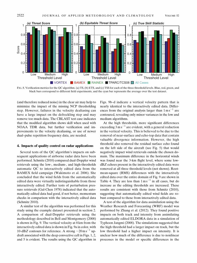
b. Skill metrics

A variety of metrics are available to assess the skill of a

dichotomous algorithm. The threat score (TS; Schaefer

1990) quantifies how well weather identification by the

algorithm corresponds to weather identification by the

experienced radar meteorologists. The TS ranges from

0 (no skill) to 1 (perfect algorithm) and is calculated by

dividing the number of hits by the total number of hits,

misses, and false positives. Figure 8a shows the TS for all

TABLE 3. Date, time, field experiment, and brief description of the cases in the verification dataset.

Date Time period (UTC) Field experiment Description

16 May 1995 2219:44–2225:59 VORTEX Tornadic supercell

23 Jun 2003 0251:00–0301:59 BAMEX Mesocyclone in mesoscale convective system

22 Sep 2005 1800:00–1821:59 RAINEX Mature hurricane eyewall

14 Sep 2008 2347:02–2355:59 T-PARC/TCS08 Tropical predepression convection


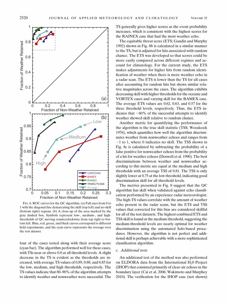
four of the cases tested along with their average score

(cyan bar). The algorithm performed well for these cases,

with TSs near or above 0.8 at all threshold levels. A slight

decrease in the TS is evident as the thresholds are in-

creased, with average TS values of 0.89, 0.88, and 0.85 for

the low, medium, and high thresholds, respectively. The

TS values indicate that 80–90%of the algorithm attempts

to identify weather and nonweather were successful. The

TS generally gives higher scores as the event probability

increases, which is consistent with the highest scores for

the RAINEX case that had the most weather echo.

The equitable threat score (ETS; Gandin andMurphy

1992) shown in Fig. 8b is calculated in a similar manner

to the TS, but is adjusted for hits associated with random

chance. The ETS was developed so that scores could be

more easily compared across different regimes and ac-

count for climatology. For the current study, the ETS

makes adjustments for higher hits from random identi-

fication of weather when there is more weather echo in

a radar scan. The ETS is lower than the TS for all cases

after accounting for random hits but shows similar rela-

tive magnitudes across the cases. The algorithm exhibits

decreasing skill with higher thresholds for the oceanic and

VORTEX cases and varying skill for the BAMEX case.

The average ETS values are 0.62, 0.63, and 0.57 for the

three threshold levels, respectively. Thus, the ETS in-

dicates that ;60% of the successful attempts to identify

weather showed skill relative to random chance.

Another metric for quantifying the performance of

the algorithm is the true skill statistic (TSS; Woodcock

1976), which quantifies how well the algorithm discrimi-

nates weather from nonweather echoes and ranges from

21 to 1, where 0 indicates no skill. The TSS shown in

Fig. 8c is calculated by subtracting the probability of a

false positive for nonweather echoes from the probability

of a hit for weather echoes (Doswell et al. 1990). The best

discriminations between weather and nonweather ac-

cording to this metric are equal at the medium and high

thresholds with an average TSS of 0.81. The TSS is only

slightly lower at 0.75 at the low threshold, indicating good

discrimination skill for all threshold levels.

The metrics presented in Fig. 8 suggest that the QC

algorithm has skill when validated against echo classifi-

cation performed by an experience radar meteorologist.

The high-TS values correlate with the amount of weather

echo present in the radar scans, but the ETS and TSS

values that corrected for this bias are considered skillful

for all of the test datasets. The highest combinedETS and

TSS skill is found at themedium threshold, suggesting the

medium-threshold levels are nearly optimal for weather

discrimination using the automated Solo-based proce-

dures. However, the algorithm is not perfect and addi-

tional skill is perhaps achievable with amore sophisticated

classification algorithm.

c. Additional tests

An additional test of the method was also performed

on ELDORA data from the International H20 Project

(IHOP) that consisted primarily of clear-air echoes in the

boundary layer (Cai et al. 2006; Wakimoto and Murphey

2010). The verification for the IHOP case (not shown)

FIG. 6. ROC curves for the QC algorithm. (a) Full axes from 0 to

1 with the diagonal line demarcating the skill (top left) and no-skill

(bottom right) regions. (b) A close-up of the area marked by the

gray dashed box. Symbols represent low-, medium-, and high-

thresholds of QC moving counterclockwise from top right to bot-

tom left. Blue, red, green, and black curves correspond to different

field experiments, and the cyan curve represents the average over

the test dataset.


was considerably poorer than the convective cases and

showed little or negative skill, depending on threshold

levels. The poor performance by the algorithm on the

IHOP case can be primarily attributed to the removal of

high-SW and low-dBZ echoes, or to the high SW/dBZ

ratio (cf. Fig. 3d). The IHOP counterexample emphasizes

the fact that the current version of the QC algorithm was

designed for precipitating convection, and should be used

with caution in other meteorological situations, particu-

larly in turbulent clear-air returns.

A modified version of the algorithm was also tested

using NOAA TDR data from the 2003 Coupled Bound-

ary Layers Air–Sea Transfer (CBLAST) experiment

during Hurricane Isabel (Bell and Montgomery 2008;

Bell et al. 2012). The algorithm required modification

because the NOAATDR data did not contain the NCP

parameter and significant velocity dealiasing was present

in the test dataset. Replacing the NCP thresholding

[step (ii) in Table 1] with a Bargen and Brown (1980)

dealiasing step provided a simplemodificationwithwhich

to test the algorithm using a NOAA TDR dataset. The

skill scores were generally consistent with the ELDORA

convective cases despite the algorithm modification and

different radar characteristics. TS valueswere near 0.9 for

all three thresholds, and ETS values ranged from 0.51 at

the high threshold to 0.57 at the low threshold. TSS values

were the best for the high threshold at 0.68, and were

similar for the medium (0.60) and low (0.63) thresholds.

Though the NCP parameter is not recorded, the

NOAATDRdata have significantly less data in the clear-

air regions than ELDORA because of the reduced sen-

sitivity of the radar receiver. The reduced data coverage

FIG. 7. PDFs and CDFs for the QC algorithm. PDFs of (a) weather echoes retained and (b) nonweather echoes

removed from the test dataset. CDFs of (c) weather echoes removed and (d) nonweather echoes retained. Dashed

green, solid blue, and dash–dotted red lines represent the low-, medium-, and high-threshold levels, respectively.


(and therefore reduced noise) in the clear air may help to

minimize the impact of the missing NCP thresholding

step. However, failures in the velocity dealiasing can

have a large impact on the defreckling step and may

remove too much data. The CBLAST test case indicates

that the modified algorithm shows skill when used with

NOAA TDR data, but further verification and im-

provements to the velocity dealiasing, or use of newer

dual–pulse repetition frequency data, are needed.

4. Impacts of quality control on radar applications

Several tests of the QC algorithm’s impacts on sub-

sequent applications of airborne radar data have been

performed. Schmitz (2010) compared dual-Doppler wind

retrievals using the low-, medium-, and high-thresholds

automatic QC to interactively edited data from the

BAMEX field campaign (Wakimoto et al. 2006). She

concluded that the wind fields from the automatically

edited data were virtually indistinguishable from those

interactively edited. Further tests of perturbation pres-

sure retrievals (Gal-Chen 1978) indicated that the auto-

matically edited data had good, if not better, momentum

checks in comparison with the interactively edited data

(Schmitz 2010).

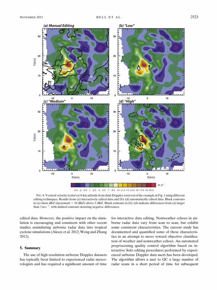
A similar test of the algorithm was performed for this

study using the example dataset presented in section 2.

A comparison of dual-Doppler retrievals using the

methodology described in Bell and Montgomery (2008)

is shown in Fig. 9. The vertical velocity at 8 km from the

interactively edited data is shown in Fig. 9a in color, with

10-dBZ contours for reference. A strong ;20ms21 up-

draft associated with the deep convective cell in Figs. 1, 2,

and 5 is evident. The results using the QC algorithm in

Figs. 9b–d indicate a vertical velocity pattern that is

nearly identical to the interactively edited data. Differ-

ences from the original analysis larger than 1ms21 are

contoured, revealing only minor variances in the low and

medium algorithms.

At the high thresholds, more significant differences

exceeding 3m s21 are evident, with a general reduction

in the vertical velocity. This is believed to be due to the

removal of near-surface and echo-top data that contain

valuable divergence information. However, the high

threshold also removed the residual surface echo found

on the left side of the aircraft (see Fig. 5) that would

negatively impact wind retrievals outside the chosen do-

main. The maximum difference in the horizontal winds

was found near the 3-km flight level, where some low-

dBZ echoes present in the interactively edited data were

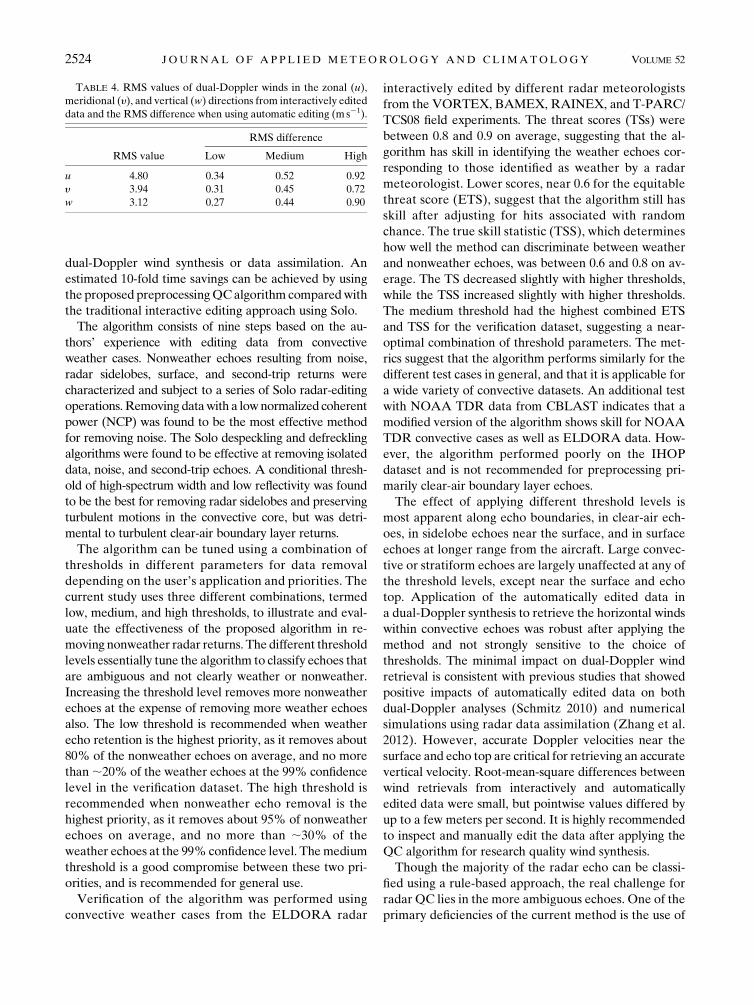
removed at all three threshold levels (not shown). Root-

mean-square (RMS) differences with the interactively

edited data over the entire domain of Fig. 9 are shown in

Table 4. They are less than 1ms21 in all cases, but do

increase as the editing thresholds are increased. These

results are consistent with those from Schmitz (2010),

suggesting that automatically edited wind fields are ro-

bust compared to those from interactively edited data.

A test of the algorithm for data assimilation using the

Weather Research and Forecasting (WRF) model was

performed by Zhang et al. (2012). They found positive

impacts on both track and intensity from assimilating

automatically edited ELDORA data in a simulation of

Typhoon Jangmi (2008). The simulations suggested that

the high threshold had a larger impact on track, but the

low threshold had a higher impact on intensity. It is

unclear how much of the difference is due to nonlinear

processes in the model or specific differences in the

FIG. 8. Verification metrics for the QC algorithm. (a) TS, (b) ETS, and (c) TSS for each of the three threshold levels. Blue, red, green, and

black bars correspond to different field experiments, and the cyan bar represents the average over the test dataset.


edited data. However, the positive impact on the simu-

lation is encouraging and consistent with other recent

studies assimilating airborne radar data into tropical

cyclone simulations (Aksoy et al. 2012;Weng andZhang

2012).

5. Summary

The use of high-resolution airborne Doppler datasets

has typically been limited to experienced radar meteo-

rologists and has required a significant amount of time

for interactive data editing. Nonweather echoes in air-

borne radar data vary from scan to scan, but exhibit

some consistent characteristics. The current study has

documented and quantified some of these characteris-

tics in an attempt to move toward objective classifica-

tion of weather and nonweather echoes. An automated

preprocessing quality control algorithm based on in-

teractive Solo editing procedures performed by experi-

enced airborne Doppler data users has been developed.

The algorithm allows a user to QC a large number of

radar scans in a short period of time for subsequent

FIG. 9. Vertical velocity (color) at 8-kmaltitude fromdual-Doppler retrieval of the example in Fig. 1 using different

editing techniques. Results from (a) interactively edited data and (b)–(d) automatically edited data. Black contours

in (a) show dBZ (increment5 10 dBZ) above 5 dBZ. Black contours in (b)–(d) indicate differences from (a) larger

than 1m s21, with dashed contours denoting negative differences.


dual-Doppler wind synthesis or data assimilation. An

estimated 10-fold time savings can be achieved by using

the proposed preprocessingQCalgorithm comparedwith

the traditional interactive editing approach using Solo.

The algorithm consists of nine steps based on the au-

thors’ experience with editing data from convective

weather cases. Nonweather echoes resulting from noise,

radar sidelobes, surface, and second-trip returns were

characterized and subject to a series of Solo radar-editing

operations.Removing datawith a lownormalized coherent

power (NCP) was found to be the most effective method

for removing noise. The Solo despeckling and defreckling

algorithms were found to be effective at removing isolated

data, noise, and second-trip echoes. A conditional thresh-

old of high-spectrum width and low reflectivity was found

to be the best for removing radar sidelobes and preserving

turbulent motions in the convective core, but was detri-

mental to turbulent clear-air boundary layer returns.

The algorithm can be tuned using a combination of

thresholds in different parameters for data removal

depending on the user’s application and priorities. The

current study uses three different combinations, termed

low, medium, and high thresholds, to illustrate and eval-

uate the effectiveness of the proposed algorithm in re-

moving nonweather radar returns. The different threshold

levels essentially tune the algorithm to classify echoes that

are ambiguous and not clearly weather or nonweather.

Increasing the threshold level removes more nonweather

echoes at the expense of removing more weather echoes

also. The low threshold is recommended when weather

echo retention is the highest priority, as it removes about

80% of the nonweather echoes on average, and no more

than;20% of the weather echoes at the 99% confidence

level in the verification dataset. The high threshold is

recommended when nonweather echo removal is the

highest priority, as it removes about 95% of nonweather

echoes on average, and no more than ;30% of the

weather echoes at the 99%confidence level. Themedium

threshold is a good compromise between these two pri-

orities, and is recommended for general use.

Verification of the algorithm was performed using

convective weather cases from the ELDORA radar

interactively edited by different radar meteorologists

from the VORTEX, BAMEX, RAINEX, and T-PARC/

TCS08 field experiments. The threat scores (TSs) were

between 0.8 and 0.9 on average, suggesting that the al-

gorithm has skill in identifying the weather echoes cor-

responding to those identified as weather by a radar

meteorologist. Lower scores, near 0.6 for the equitable

threat score (ETS), suggest that the algorithm still has

skill after adjusting for hits associated with random

chance. The true skill statistic (TSS), which determines

how well the method can discriminate between weather

and nonweather echoes, was between 0.6 and 0.8 on av-

erage. The TS decreased slightly with higher thresholds,

while the TSS increased slightly with higher thresholds.

The medium threshold had the highest combined ETS

and TSS for the verification dataset, suggesting a near-

optimal combination of threshold parameters. The met-

rics suggest that the algorithm performs similarly for the

different test cases in general, and that it is applicable for

a wide variety of convective datasets. An additional test

with NOAA TDR data from CBLAST indicates that a

modified version of the algorithm shows skill for NOAA

TDR convective cases as well as ELDORA data. How-

ever, the algorithm performed poorly on the IHOP

dataset and is not recommended for preprocessing pri-

marily clear-air boundary layer echoes.

The effect of applying different threshold levels is

most apparent along echo boundaries, in clear-air ech-

oes, in sidelobe echoes near the surface, and in surface

echoes at longer range from the aircraft. Large convec-

tive or stratiform echoes are largely unaffected at any of

the threshold levels, except near the surface and echo

top. Application of the automatically edited data in

a dual-Doppler synthesis to retrieve the horizontal winds

within convective echoes was robust after applying the

method and not strongly sensitive to the choice of

thresholds. The minimal impact on dual-Doppler wind

retrieval is consistent with previous studies that showed

positive impacts of automatically edited data on both

dual-Doppler analyses (Schmitz 2010) and numerical

simulations using radar data assimilation (Zhang et al.

2012). However, accurate Doppler velocities near the

surface and echo top are critical for retrieving an accurate

vertical velocity. Root-mean-square differences between

wind retrievals from interactively and automatically

edited data were small, but pointwise values differed by

up to a few meters per second. It is highly recommended

to inspect and manually edit the data after applying the

QC algorithm for research quality wind synthesis.

Though the majority of the radar echo can be classi-

fied using a rule-based approach, the real challenge for

radar QC lies in the more ambiguous echoes. One of the

primary deficiencies of the current method is the use of

TABLE 4. RMS values of dual-Doppler winds in the zonal (u),

meridional (y), and vertical (w) directions from interactively edited

data and the RMS difference when using automatic editing (ms21).

RMS value

RMS difference

Low Medium High

u 4.80 0.34 0.52 0.92

y 3.94 0.31 0.45 0.72

w 3.12 0.27 0.44 0.90


hard thresholds for each of the discriminating parame-

ters. A more sophisticated algorithm must take into ac-

count the ‘‘fuzzy’’ nature of the radar echoes in different

scanning strategies and meteorological situations. For

example, it is evident that the probability of weather

generally increases as the NCP increases, but use of this

single parameter does not contain enough information

to define an optimal threshold for all situations. The

classification must ultimately be multidimensional and

requires more complex logic that is not possible within

the Solo framework. Furthermore, the classification is

currently subjective and could be improved with better

objective characterization of nonweather echoes using

synthetic datasets. The medium threshold represents

a near-optimal set of thresholds for meeting both re-

quirements of removing nonweather and retaining

weather echoes identified by a radar meteorologist using

Solo. However, further refinement appears to be possible

outside the confines of the Solo software. Continued de-

velopment of the method to incorporate multidimen-

sional fuzzy logic in a stand-alone software package is

currently under way.

Acknowledgments. This research was funded by the

National Science Foundation through the American Re-

covery and Reinvestment Act. The first author was also

partially supported by NSF Award AGS-0851077 and the

Office of Naval Research Award N001408WR20129. The

authors also thank Cathy Kessinger and Andy Penny for

their comments on the manuscript.

APPENDIX A

Solo Interactive Radar Editor

Solo was originally developed at NCAR in 1993 for

perusing and editing Doppler radar data (Oye et al.

1995), and was extensively revised in version 2 (also re-

ferred to as SoloII) in 2003. The title of the software is not

an acronymbut rather stems from the initial development

location in the Solomon Islands as part of the Tropical

Ocean Global Atmosphere (TOGA) Coupled Ocean–

Atmosphere Response Experiment (COARE) field

program. The native data format for Solo is Doppler

Radar Data Exchange (DORADE; Lee et al. 1994b)

developed for ELDORA, with individual DORADE

files colloquially known as ‘‘sweep files.’’ ELDORA

data editing is typically done by the principal investigator

for a field project as part of their postexperiment research

with assistance fromNCAR,where editing procedures can

be tuned based on the specific project requirements. Solo

has been the primary editing software formanyELDORA

and NOAA tail Doppler radar users over the years.

The Solo data viewer can display up to 12 color panels

of different radar field variables with range rings or

Cartesian distance overlays. The numerical values of in-

dividual radar gates can be inspected using the ‘‘Data’’

widget. A more detailed inspection of the data can be

performed using the ‘‘Examine’’ widget, which can dis-

play numerical values of multiple data fields in a specified

area, the metadata associated with the radar data header,

or the history of radar edits in the file. The Examine

widget can also be used for point-and-click deletion or

velocity unfolding of individual radar gates or rays.

Both interactive and bulk radar data editing can be

performed using the ‘‘Editor’’ widget. In an interactive

setting, the user can draw a boundary around an arbi-

trarily defined patch of radar echo and apply a series of

operators to that patch on a scan-by-scan basis. In a batch

mode, editing operations can be applied tomultiple radar

scans at one time. Many editing operations are available

for ground-based and airborne platforms, ranging from

simple deletion to more complex series of logical opera-

tions. Solo also contains several diagnostic operators in-

cluding histogram, rain-rate, and radial shear calculations.

The primary operators used for the QC algorithm pre-

sented in this study are the ‘‘remove surface,’’ ‘‘thresh-

old,’’ ‘‘despeckle,’’ and ‘‘defreckle’’ operators. Ground

removal operations use the aircraft altitude, aircraft

attitude parameters, radar beamwidth, and the radar-

pointing angles to identify potential surface returns. At

the present time, Solo cannot handle complex terrain.

Threshold operations remove data in one field based on

the numerical values exceeding a specified parameter

in another field. Data removal can be performed above,

below, or between the specified threshold values. The

despeckle operator removes clusters of radar gates along

a ray that are smaller than a specified ‘‘speckle’’ defini-

tion, defined by default as three gates. Therefore,

despeckling removes isolated radar gates that are not

part of a larger weather echo. Isolated gates with large

numerical values that are embedded within a weather

echo can be identified by comparison with the average

value of nearby radar gates. An outlier algorithm to

identify these gates is implemented in the radial di-

rection as the defreckle algorithm, and in a circular patch

as a ‘‘deglitch’’ algorithm. Experiments for the current

study with the deglitch operator tended to remove more

data compared than the defreckle operator.

Other Solo editing operators include velocity deal-

iasing using the Bargen and Brown (1980) algorithm and

mathematical functions (i.e., add, subtract, multiply, and

exponentiate). Solo can also be used to correct radar

metadata such as aircraft inertial navigation system errors

(Testud et al. 1995; Bosart et al. 2002). Earth-relative

Doppler velocities and radar gate locations can then be


recalculated using the corrected platform location and

motion.

One deficiency of the SoloII software is that it depends

on an older, deprecated 32-bit graphics library, and the

code is not easily accessible for modification to add or

improve the available editing steps. A stand-alone ver-

sion of the batch-editing functionality of the software has

been developed by the authors. The stand-alone version

has an easily modified Ruby script interface, but it cur-

rently lacks the full functionality of Solo as a data viewer

and interactive editor. Efforts to upgrade to version 3 of

Solo, including full 64-bit support, are currently under

way at NCAR. The Solo software package, editing

scripts described here, and stand-alone editing soft-

ware are available for interested users.

APPENDIX B

Automated Quality Control Procedures

This appendix presents in detail the steps that are

listed in Table 1, with steps viii and ix combined in the

last section.

a. Backup original reflectivity and velocity fields

The current version 2 of Solo does not have an ‘‘undo’’

functionality. As a result, it is important for any editing

step using this software to store the results of unedited or

stepwise-edited procedures that could result in unwanted

loss of data. This step alsomakes it easy to apply different

levels of thresholding within the same file under different

data field names.

b. Remove noisy data with low NCP

The NCP parameter is a normalized value between

zero and one representing a spectrum from pure noise to

strong signal in the Doppler velocity estimate as de-

scribed in section 2. The three thresholds selected for the

automatic algorithm range from 0.2 to 0.4, above which

the removal of quality weather data becomes unaccept-

able for most applications. While the NCP threshold is

relatively simple, it removes the most data of any step in

the algorithm. Noisy gates that remain after this step are

typically isolated and are further addressed in section f of

appendix B. The NCP parameter is not currently com-

puted in NOAA TDR data, and therefore this step is not

applicable for NOAA TDR datasets.

c. Remove noisy data near the edges of radar range

The data from the first few gates near the aircraft of-

ten have strong dBZ and noisy Doppler velocities due to

saturation of the receiver, as is evident in Fig. 2. Similarly,

data in the last few gates at the edge of the radar range are

often unusable due to signal-processing requirements

(e.g., test pulse). While the amount of noise is dependent

on the meteorological conditions and the unambiguous

range of the radar, the limited number of gates retained

by a careful examination of these regions is usually not

worth the effort. Approximately five gates at the begin-

ning and end of each radar beam are therefore removed

in this algorithm step, which can be adjusted as needed.

d. Remove the direct surface returns

Testud et al. (1995) derived a formula to identify the

radar gates contaminated by the surface echo based

on the half-power beamwidth of the radar antenna. An

increase in the ‘‘effective’’ width of the radar beam is

sufficient to identify and remove gates with partial

beamfilling in the surface identification algorithm. The

low threshold uses an effective beamwidth parameter of

28 that is slightly above the native resolution of ELDORA

and NOAA TDR (1.88). Higher effective beamwidths of

38 and 48 at the medium and high thresholds remove

substantiallymore surface echo, especially away from the

nadir rotation angle. At longer ranges, the high threshold

may remove too much near-surface echo and should be

used with caution when quality vertical velocity estimates

are important.

e. Remove data with high SW and low dBZ

The ratio of the SW and dBZ fields is analogous to

the NCP parameter, with the variance of the Doppler

signal used instead of the power in the velocity signal.

In this step, volumes with SW greater than 6m s21 and

dBZ less than zero are removed at the low-threshold

level. The SW threshold is decreased to 4m s21 at the

medium level, and the dBZ threshold is increased to 5

at the high level.

For radars that do not record NCP, this step can serve

as a proxy for the step described in section b of ap-

pendix B. The caveat with the SW–dBZ threshold is that

regions of turbulence or wind shear with small scatterers

will be adversely affected. The thresholds were chosen to

remove sidelobe echoes and minimize the chance of

convective turbulence being removed by the algorithm.

However, tests indicate that this step can remove signif-

icant echo from the clear-air boundary layer and should

be used with caution when preservation of boundary

layer echoes is important.

f. Despeckle the data

The spatial scales of the weather observed by airborne

Doppler radars are typically much larger than individual

radar range gates. After the previous five steps have been

performed, the majority of the nonweather echoes have

been removed and the remaining isolated gates with few


neighbors are unlikely to represent significant meteoro-

logical features. An efficient algorithm for identifying

speckles, or isolated gates along the radar beam, is part of

the Solo editor with a variable definition for the speckle

size. The low threshold uses the default speckle definition

of three gates, effectively removing features with spatial

scales less than 450m (for a 150-m-range gate). The me-

dium and high thresholds increase the definition to five

and seven gates, or 750 and 1050m, respectively.

Unfortunately, the corresponding algorithm for iden-

tifying isolated gates in the azimuthal direction is not part

of the Solo package. Thus, a larger speckle definition has

the potential to remove features that are relatively thin

in the radial direction but have significant horizontal ex-

tent. The most common examples of this are the anvil

region of a thunderstorm or shallow, near-surface struc-

tures such as boundary layer clouds or insect returns.

Careful consideration of the features of interest is impor-

tant for determining the speckle definition.

g. Defreckle the data

Complementary to radar speckles are radar freckles.

Freckles are radar gates that are outliers relative to their

neighbors within a larger weather echo. A freckle can be

defined as a gate with a value that deviates significantly

from a spatial mean in the neighborhood of the gate.

Though the freckles can be defined using any radar pa-

rameter, only the Doppler velocity is used in the current

algorithm. Because this step is primarily for outlier de-

tection, the freckle definitions are identical for the three

threshold levels with a five-gate running mean and a

20m s21 outlier criterion.

In general, the defreckling algorithm is effective at

removing spikes in the velocity field within weather

echoes while retaining realistic velocity gradients. The

defreckle algorithm is also effective at removing second-

trip echoes that havemoderate dBZ but randomDoppler

velocities. A potential failure mode of the defreckle

algorithm occurs when the mean becomes ill-defined

relative to the outliers. This appears to occur most of-

ten where a second-trip echo occurs radially inward of

a weather echo. The running mean is then defined by

noisy data and the entire beam can be removed. The

algorithm can also fail where there is a strong velocity

gradient across a region ofmissing data such as that found

between hurricane rainbands, or where the velocity has

aliasing errors.

h. Second despeckling and synchronization ofreflectivity and velocity

A final pass with the despeckling algorithm removes

any gates that were isolated by the defreckling algorithm,

and the synchronization ensures that identical gates are

removed from both the dBZ and velocity fields. The

synchronization is not ideal, because the reflectivity may

be representative of weather even when the velocity is

noisy. Unfortunately, the algorithm cannot distinguish

this situation because the primary criteria are based on

velocity metrics.

REFERENCES

Aksoy, A., S. Lorsolo, T. Vukicevic, K. J. Sellwood, S. D. Aberson,

and F. Zhang, 2012: The HWRF Hurricane Ensemble Data

Assimilation System (HEDAS) for high-resolution data: The

impact of airborne Doppler radar observations in an OSSE.

Mon. Wea. Rev., 140, 1843–1862.Bargen, D. W., and R. C. Brown, 1980: Interactive radar velocity

unfolding. Preprints, 19th Conf. on RadarMeteorology,Miami

Beach, FL, Amer. Meteor. Soc., 278–285.

Bell, M. M., and M. T. Montgomery, 2008: Observed structure,

evolution, and potential intensity of category 5 Hurricane

Isabel (2003) from 12 to 14 September.Mon.Wea. Rev., 136,

2023–2045.

——, and——, 2009: Airborne radar observations of pre-depression

Hagupit during TPARC/TCS-08. Preprints, 34th Conf. on

Radar Meteorology, Williamsburg, VA, Amer. Meteor. Soc.,

12A.5. [Available online at https://ams.confex.com/ams/

34Radar/techprogram/paper_156070.htm.]

——, ——, and K. E. Emanuel, 2012: Air–sea enthalpy and mo-

mentum exchange at major hurricane wind speeds observed

during CBLAST. J. Atmos. Sci., 69, 3197–3222.

Bosart, B. L.,W.-C. Lee, andR.M.Wakimoto, 2002: Procedures to

improve the accuracy of airborneDoppler radar data. J. Atmos.

Oceanic Technol., 19, 322–339.

Bousquet, O., and B. F. Smull, 2003: Airflow and precipitation

fields within deep alpine valleys observed by airborneDoppler

radar. J. Appl. Meteor., 42, 1497–1513.

Cai, H., W.-C. Lee, T. M. Weckwerth, C. Flamant, and H. V.

Murphey, 2006: Observations of the 11 June dryline during

IHOP_2002—A null case for convection initiation. Mon.

Wea. Rev., 134, 336–354.

Doswell, C. A., III, R. Davies-Jones, and D. L. Keller, 1990:

On summary measures of skill in rare event forecasting based

on contingency tables. Wea. Forecasting, 5, 576–585.

Frush, C., R. J. Doviak, M. Sachidananda, and D. S. Zrnic, 2002:

Application of the SZ phase code to mitigate range–velocity

ambiguities in weather radars. J. Atmos. Oceanic Technol., 19,

413–430.

Gal-Chen, T., 1978: A method for the initialization of the anelastic

equations: Implications for matching models with observa-

tions. Mon. Wea. Rev., 106, 587–606.

Gamache, J. F., 2005: Real-time dissemination of hurricane wind

fields determined from airborne Doppler radar data. Joint

Hurricane Testbed Final Rep., U.S. Weather Research Pro-

gram, 12 pp. [Available online at http://www.nhc.noaa.gov/jht/

2003-2005reports/DOPLRgamache_JHTfinalreport.pdf.]

Gandin, L., and A. H. Murphy, 1992: Equitable skill scores for

categorical forecasts. Mon. Wea. Rev., 120, 361–370.

Georgis, J. F., F. Roux, and P. H. Hildebrand, 2000: Observation of

precipitating systems over complex orography with meteoro-

logical Doppler radars: A feasibility study. Meteor. Atmos.

Phys., 72, 185–202.


https://ams.confex.com/ams/34Radar/techprogram/paper_156070.htm

https://ams.confex.com/ams/34Radar/techprogram/paper_156070.htm

http://www.nhc.noaa.gov/jht/2003-2005reports/DOPLRgamache_JHTfinalreport.pdf

http://www.nhc.noaa.gov/jht/2003-2005reports/DOPLRgamache_JHTfinalreport.pdf

Hildebrand, P. H., and Coauthors, 1996: The ELDORA/ASTRAIA

airborne Doppler weather radar: High-resolution observa-

tions from TOGA COARE. Bull. Amer. Meteor. Soc., 77,

213–232.

Houze, R. A., Jr., and Coauthors, 2006: The Hurricane Rainband

and Intensity Change Experiment: Observations and modeling

of Hurricane Katrina, Ophelia, and Rita. Bull. Amer. Meteor.

Soc., 87, 1503–1521.Joliffe, I. T., and D. B. Stephenson, 2003: Forecast Verification:

A Practitioner’s Guide in Atmospheric Science. John Wiley

and Sons, 254 pp.

Jorgensen, D. P., T. R. Shepherd, and A. S. Goldstein, 2000:

A dual-pulse repetition frequency scheme for mitigating

velocity ambiguities of theNOAAP-3 airborneDoppler radar.

J. Atmos. Oceanic Technol., 17, 585–594.

Lakshmanan, V., A. Fritz, T. Smith, K. Hondl, and G. J. Stumpf,

2007: An automated technique to quality control radar re-

flectivity data. J. Appl. Meteor., 46, 288–305.

Lee, W.-C., P. Dodge, F. D. Marks, and P. H. Hildebrand, 1994a:

Mapping of airborne Doppler radar data. J. Atmos. Oceanic

Technol., 11, 572–578.

——, C. Walther, and R. Oye, 1994b: Doppler Radar Data Ex-

change format DORADE. National Center for Atmospheric

Research Tech. Rep., 18 pp.

——, F. D. Marks, and C. Walther, 2003: Airborne Doppler Radar

Data Analysis Workshop. Bull. Amer. Meteor. Soc., 84, 1063–

1075.

Oye, R., C. Mueller, and S. Smith, 1995: Software for radar trans-

lation, visualization, editing, and interpolation. Preprints, 27th

Conf. on Radar Meteorology, Vail, CO, Amer. Meteor. Soc.,

359–361.

Sachidananda, M., and D. Zrnic, 1999: Systematic phase codes for

resolving range overlaid signals in a Doppler weather radar.

J. Atmos. Oceanic Technol., 16, 1351–1363.

Schaefer, J. T., 1990: The critical success index as an indicator of

warning skill. Wea. Forecasting, 5, 570–575.

Schmitz, A., 2010: An investigation to address the robustness of

aircraft radar data. M.S. thesis, Dept. of Meteorology, St. Louis

University, 188 pp.

Stanski, H. R., L. J. Wilson, and W. R. Burrows, 1989: Survey of

common verification methods in meteorology. World Meteo-

rological Organization World Weather Watch Tech. Rep. 8,

114 pp.

Steiner, M., and J. A. Smith, 2002: Use of three-dimensional

reflectivity structure for automated detection and removal

of nonprecipitating echoes in radar data. J. Atmos. Oceanic

Technol., 19, 673–686.

Testud, J., P. H. Hildebrand, and W.-C. Lee, 1995: A procedure to

correct airborne Doppler radar data for navigation errors using

the echo returned from the earth’s surface. J. Atmos. Oceanic

Technol., 12, 800–820.Wakimoto, R. M., and H. V. Murphey, 2010: Frontal and radar

refractivity analyses of the dryline on 11 June 2002 during

IHOP. Mon. Wea. Rev., 138, 228–241.

——, C. Liu, and H. Cai, 1998: The Garden City, Kansas, storm

during VORTEX 95. Part I: Overview of the storm’s life cycle

and mesocyclogenesis. Mon. Wea. Rev., 126, 372–392.

——, H. Cai, and H. V. Murphey, 2004: The Superior, Nebraska,

supercell during BAMEX.Bull. Amer. Meteor. Soc., 85, 1095–1106.

——,H. V.Murphey, A. Nester, D. P. Jorgensen, and N. T. Atkins,

2006: High winds generated by bow echoes. Part I: Overview

of the Omaha bow echo 5 July 2003 storm during BAMEX.

Mon. Wea. Rev., 134, 2793–2812.

Weng, Y., and F. Zhang, 2012: Assimilating airborne Doppler radar

observations with an ensemble Kalman filter for convection-

permitting hurricane initialization and prediction: Katrina

(2005). Mon. Wea. Rev., 140, 841–859.

Woodcock, F., 1976: The evaluation of yes/no forecasts for scientific

and administrative purposes. Mon. Wea. Rev., 104, 1209–1214.Zhang, L., Z. Pu, W.-C. Lee, and Q. Zhao, 2012: The influence of

airborne Doppler radar data quality on numerical simulations

of a tropical cyclone. Wea. Forecasting, 27, 231–239.


a solo-based automated quality control algorithm for ... · a solo-based automated quality control...

Documents