a simulated annealing approach for the minmax regret path ... · averbakh (pereira and averbakh,...

September 24-28, 2012Rio de Janeiro, Brazil

A Simulated Annealing Approach for the Minmax Regret PathProblem

Francisco Pérez, César A. Astudillo, Matthew Bardeen, Alfredo Candia-Vé[email protected], {castudillo, mbardeen, acandia}@utalca.cl

Universidad de TalcaKm 1. Camino a los Niches Curicó, Chile

August 5, 2012

Abstract

We propose a novel neighbor generation method for a Simulated Annealing (SA) algorithmused to solve the Minmax Regret Path problem with Interval Data, a difficult problem in Com-binatorial Optimization. The problem is defined on a graph where there exists uncertainty in theedge lengths; it is assumed that the uncertainty is deterministic and only the upper and lowerbounds are known. A worst-case criterion is assumed for optimization purposes. The goal isto find a path s-t, which minimizes the maximum regret. The literature includes algorithmsthat solve the classic version of the shortest paths problem efficiently. However, the variant thatwe study in this manuscript is known to be NP-Hard. We propose a SA algorithm to tacklethe aforementioned problem, and we show that our implementation is able to find good solu-tions in reasonable times for large size instances. Furthermore, a known exact algorithm thatutilizes a Mixed Integer Programming (MIP) formulation was implemented by using a com-mercial solver (CPLEX1). We show that this MIP formulation is able to solve instances up to1000 nodes within a reasonable amount of time.

1 Introduction

In this work we study a variant of the well known Shortest Path (SP) problem. For the classicalversion of this problem, efficient algorithms have been known since 1959 (Dijkstra, 1959). Givena digraph G = (V,A) (V is the set of nodes and A is the set of arcs) with non-negative arc costsassociated to each arc and two nodes s and t in V , SP consists of finding a s-t path of minimum totalcost. Dijkstra designed a polynomial time algorithm and from this, a number of other approacheshave been proposed. Ahuja et al. present the different algorithmic alternatives to solve the problem(Ahuja et al., 1993).

Our interest is focused on the variant of shortest path problems where there exists uncertaintyin the objective function parameters. In this SP problem, for each arc we have a closed intervaldefining the possibilities for the arc length. A scenario is a vector where each number represents oneelement of an arc length interval. The uncertainty model used here is the minmax regret approach(MMR), sometimes named robust deviation; in this model the problem is to find a feasible solutionbeing α-optimal for any possible scenario with α as small as possible. One of the properties of theminmax regret model is that it is not as pessimistic as the (absolute) minmax model. This model

1Although popularly referred to simply as CPLEX, its formal name is IBM ILOG CPLEX Optimization Studio.For additional information, the interested reader may consult the following URL: http://www-01.ibm.com/software/integration/optimization/cplex-optimizer/

1

2332


in combinatorial optimization has largely been studied only recently: see the books by Kouvelisand Yu (Kouvelis and G., 1997), and Kasperski (Kasperski, 2008), as well as the recent reviews byAissi et al. (Aissi et al., 2009) and Candia-Véjar et al. (Candia-Véjar et al., 2011). The later alsomentions some interesting applications of the MMR model in the real world.

It is known that minmax regret combinatorial optimization problems with interval data (MM-RCO) are usually NP-hard, even in the case when the classic problem is easy to solve; this isthe case of the minimum spanning tree problem, shortest path problem, assignment problems andothers; see Kasperski (2008) for details.

Exact algorithms for Minmax Regret Paths have been proposed by (Karasan et al., 2001; Kasper-ski, 2008; Montemanni and Gambardella, 2004, 2005). All these papers show that exact solutionsfor MMRP can be obtained by different methods and take into account several types of graphs anddegrees of uncertainty. However, the size of the graphs tested in these papers was limited to amaximum of 2000 nodes.

In this context, our main contributions in this paper are the analysis of the performance ofthe CPLEX solver for a MIP formulation of MMRP, the analysis of the performance of knownheuristics for the problem and finally the analysis of the performance of a proposed SA approach forthe problem. For experiments we consider two classes of networks, random and a class of networksused in telecommunications and both containing different problem sizes. Instances containing from500 to 20000 nodes with different degrees of uncertainty were considered.

In the next section, we present the formal definition of the problem and notation associated andin Section 3 a mathematical programming formulation for MMRP is presented. We also discuss themidpoint scenario and the upper limit scenario heuristics for MMRP in more detail and then presentthe general algorithm for SA. In Section 4 we formally define the neighborhood used for our SAapproach. Details of our experiments and their results are analyzed in Section 5. Finally in Section6, our conclusions and suggestions for future work are presented.

2 Notation and Problem Definition

LetG = (V,A) be a digraph, where V corresponds to the set of vertices and A is conformed by a setof arcs. With each arc (i, j) in A we associate a non-negative cost interval [c−ij , c

+ij ], c

−ij ≤ c+ij , i.e.,

there is uncertainty regarding the true cost of the arc (i, j), and whose value is a real number thatfalls somewhere in the above-mentioned interval. Additionally, we make no particular assumptionsregarding the probability distribution of the unknown costs.

The Cartesian product of the uncertainty intervals[c−ij , c

+ij

], (i, j)εA, is denoted as S and any

element s of S is called a scenario; S is the vector of all possible realizations of the costs of arcs.csij , (i, j)εA denote the costs corresponding to scenario s.

Let P be the set of all s-t paths in G. For each XεP and sεS, let

F (s,X) =∑

(i,j)εX

csij , (1)

be the cost of the s-t path X in the scenario s.The classical s-t shortest path problem for a fixed scenario sεS isProblem OPT.PATH(s). Minimize F (s,X) : XεP .Let F ∗(s) be the optimum objective value for problem OPT.PATH(s).For any XεP and sεS, the value R(s,X) = F (s,X)− F ∗(s) is called the regret for X under

scenario s. For any XεP , the value

Z(X) = maxsεSR(s,X), (2)

2

2333


is called the maximum (or worst-case) regret for X and an optimal scenario s∗ producing sucha worst-case regret is called worst-case scenario for X . The minmax regret version of ProblemOPT.PATH(s) is

Problem MMRP. Minimize {Z(X) : XεP} .

Let Z∗ denote the optimum objective value for Problem MMRP.For any XεP , the scenario induced by X , s(X), for each (i, j)εA is defined by

cs(X)ij =

{c+ij , (i, j) εX

c−ij , otherwise.(3)

Let Y (s) denote an optimal solution to Problem OPT.PATH(s).

Lemma 1 (Karasan et al. (Karasan et al., 2001)). s(X) is a worst-case scenario for X .

According to Lemma 1, for any XεP , the worst-case regret

Z(X) = F (s(X), X)− F ∗(s(X))

= F (s(X), X)− F (s(X), Y (s(X)), (4)

can be computed by solving just one classic SP problem according to the definition of Y (S) givenabove.

3 Algorithms for MMRP

In this section we present both a MIP formulation for MMRP, which will be used to obtain an exactsolution by using a solver CPLEX, and our SA approach for finding an approximate solution forthe problem. Two simple and known heuristics based on the definition of specific scenarios are alsopresented.

3.1 A MIP Formulation for MMRP

Consider a digraph G = (V,A) with two distinguished nodes s and t. According with the pastsection each arc (i, j) ∈ A has interval weight

[c−ij , c

+ij

]and also has a binary variable xij associated

expressing if the arc (i, j) is part of the constructed path. We use Kasperski’s MIP formulation ofMMRP (Kasperski, 2008), given as follows:

min∑

(i,j)∈A

c+ijxij − λs + λt (5)

λi ≤ λj + c+ijxij + c−ij(1− xij), (i, j) ∈ A, λ ∈ R (6)

∑{i:(j,i)∈A}

xji −∑

{k:(k,j)∈A}

xkj =

1, j = s

0, j ∈ V -{s, t}−1, j = t

(7)

xij ∈ {0, 1} , for (i, j) ∈ A (8)

The solver CPLEX is then used to solve the above MIP.

3

2334


3.2 Basic Heuristics for MMRP

Two basic heuristics for MMRP are known; in fact these heuristics are applicable to any MM-RCO problem. These heuristics are based on the idea of specifying a particular scenario and thensolving a classic problem using this scenario. The output of these heuristics are feasible solutionsfor the MMRCO problem (Candia-Véjar et al., 2011; Conde and Candia, 2007; Kasperski, 2008;Montemanni et al., 2007; Pereira and Averbakh, 2011a,b).

First we mention the midpoint scenario, sM defined as sM = [(c+e + c−e )/2] , e ∈ A. Theheuristic based on the midpoint scenario is described in Algorithm HM.

Algorithm HM(G,c)

Input: Network G, and interval costsfunction c

Output: A feasible solution Y for MMRP.1: for all e ∈ A do2: cs

M

e = (c+e + c−e )/23: end for4: Y ← OPT (sM )5: return Y, Z(Y )

Algorithm HU(G,c)

Input: Network G, and interval costsfunction c

Output: A feasible solution Y for MMRP.1: for all e ∈ A do2: cs

U

e = c+e3: end for4: Y ← OPT (sU )5: return Y,Z(Y )

We refer to the heuristic based on the midpoint scenario as HM. The other heuristic based onthe upper limit scenario will be denoted by HU and is described in Algorithm HU.

The heuristics HU and HM have been designed for rapidly obtaining feasible solutions. Theseheuristics find a solution by solving the corresponding classic problem only twice. The first is thecomputation of the solution Y in the specific scenario, sM for HM or sU for HU, and the second isthe computation of Z(Y ) (see steps 4 and 5 in Algorithm HM and Algorithm HU). These heuristicshave been used in an integrated form by the sequential computing of the solutions given by HM andHU and using the best. In the evaluation of heuristics for MMR problems, some experiments haveshown that if these heuristics are considered as an initial solution for a heuristic, improved solutionsare not easy to achieve, please refer to Montemanni et al. (Montemanni et al., 2007), Pereira andAverbakh (Pereira and Averbakh, 2011a,b) and Candia-Véjar et al. (Candia-Véjar et al., 2011) fora more detailed explanation.

3.3 Simulated Annealing for MMRP

Simulated Annealing (SA) is a very traditional metaheuristic, see Dréo et al. (2006) for details. Ageneric version of SA is specified in Kirkpatrick et al. (1983).

We shall now describe the main concepts and parameters used within the context of the MMRPproblem,

Search Space A subgraph S of the original graphG is defined such that this subgraph contains a s-t path. In S a classical s-t shortest path subproblem is solved, where the arc costs are chosentaking the upper limit arc costs. Then, the optimum solution of these problem is evaluated foracceptation.

Initial Solution The initial solution Y0 is obtained applying the heuristic HU to the original net-work S0 The regret Z(Y0) is then computed.

4

2335


Initial Temperature Different values for the initial temperature were tested and t0 = 1 was usedfor all experiments.

Cooling Programming A geometric descent of the temperature was according to parameter beta.Several experiments were performed and after to consider the trade-off between the regret ofthe solution and time needed to compute it, β was fixed as 0.94 for all experiments.

Internal Loop This loop is defined by a parameter L and depended on the size of the instancestested. After initial experiments, L was fixed at 25 for instances from 500 nodes to 10000nodes. For instances with 20000 nodes the L was fixed at 50.

Neighborhood Search Moves Let Si be the subgraph of G considered at the iteration i and let xi

be the solution given by the search space at the iteration i. Then we generate a new subgraphSi+1 of G from Si changing the status of some components of the vector characterizing Si.The number of components is managed by a parameter λ and a feasible solution is obtainingsearching Si+1 (according with the definition of Search Space) which must be tested foracceptation.

Acceptation Criterion A standard probabilistic function is used to determine if a neighboring so-lution is accepted or not.

Termination Criterion A fixed value of temperature (final temperature tf ) is used as terminationcriterion with tf = 0.01.

Our definition of Neighborhood Search Moves is new, but takes inspiration from that describedby Nikulin. In his paper (Nikulin, 2007), he applied this to the interval data minmax regret spanningtree problem.

4 Neighborhood Structure for the MMRP problem

Given the importance of the neighborhood structure in our proposed method, we have dedicated thissection to explain it in detail. We start by defining the Local Search (LS) mechanism. Subsequentlywe detail the concepts of neighborhood structure and Search Space. After that, we explicitly de-scribe an architectural model for obtaining new candidate solution by restricting the original searchspace.

4.1 Local Search (LS)

Local Search (LS), described in Algorithm local-search, is a search method for a CO problem Pwith feasible space S. The method starts from an initial solution and iteratively improves it byreplacing the current solution with a new candidate, which is only marginally different. During thisinitialization phase, the method selects an initial solution Y from the search space S . This selectionmay be at random or taking advantage of some a priori knowledge about the problem.

An essential step in the algorithm is the acceptance criterion, i.e., a neighbor is identified as thenew solution if its cost is strictly less in comparison to the current solution. This cost is a functionassumed to be known and is dependent on the particular problem. The algorithm terminates whenno improvements are possible, which happens when all the neighbors have a higher (or equal) costwhen compared to the current solution. At this juncture, the method outputs the current solution asthe best candidate. Observe that, at all iteration steps, the current solution is the best solution foundso far. LS is a sub-optimal mechanism, and it is not unusual that the output will be far from the

5

2336


optimum. The literature reports many algorithms that attempt to overcome the hurdles encounteredin the original LS strategy. The interested reader may consult (Luke, 2009) for a survey.

Algorithm local-search(S,cost(·),N(·))

Input:(i) S, A search space.(ii) cost(·), a cost function.(iii) N(·) a neighborhood function.

1: Y ← A starting solution from S.2: while ∃Y ′ ∈ N(Y ) such that cost(Y ′)< cost(Y ) do

3: Y ← Y ′

4: end while

Algorithm neighbor-induction(R)

Input: R, a subspace of the original searchspace S.

Output: Y ′, the new candidate solution.

1: R′ ← subspace-perturbation(R)2: Y ′ ← generate-candidate(R′)

4.2 Neighbor Induction Via Subspace Perturbation

Typically in LS, almost all cases of neighborhood structures are analogous to the k-opt methodexplained above, in the sense that a candidate solution is obtained by applying a slight modificationto the previous candidate. A fundamentally different philosophy is the one of using sub-spaces toinduce candidate solutions. In this model, the new candidate is not obtained directly from a previoussolution. Rather the candidate is obtained by an indirect step, which consists in perturbing a sub-space in a LS fashion so as to obtain a new subspace which is marginally different in comparisonto the former. Finally, the new subspace is employed to derive the new candidate solution. Thisconcept adds an extra layer in the architectural model for defining the neighborhood structure. Themethod is detailed in Algorithm neighbor-induction, which generalizes the method presented in(Nikulin, 2007). The author of (Nikulin, 2007), in the first step apply local transformations to aconnected graph (sub-space) to obtain a new graph which is also connected (new sub-space). In thesecond step, they calculate the differences in the regret between the original and modified candidatesolutions.

4.3 MMRP Neighborhood

Our proposed solution for the MMRP Neighborhood retains the idea of using bitmap strings torepresent (and restrict) the search space. We start by defining a bitmap string with cardinality |A|,such that π(j) = 1 if edge aj belongs to the current subset, and πi(j) = 0 otherwise. Further, π(j)denotes the bit j of the bitmap vector. The full process for creating a new search space is detailedin Algorithm MMRP-subspace-perturbation.

At each iteration, a predetermined fraction of arcs from the original subspace are inverted, i.e.,they are set to 1 (added) if they were not present in π or set to 0 (deleted) otherwise. This fractionis controlled by the parameter γ, and directly relates the concept of exploration and exploitationmentioned earlier. Small values for γ lead to slight perturbations of the current subspace, i.e., theresultant subspace will be only marginally different from the subspace currently being examined.This configuration favors the exploitation of the current solution. In contrast, large values for γproduce strong perturbations of the subspace, producing subspaces which are expected to be muchdifferent from the subspace currently being perturbed, which favors the exploration of unvisited

6

2337


regions in the original search space. Exploratory test on a variety of datasets have show evidencethat a suitable value for γ depends on the dataset being tested and particularly its size.

Once the subspace is determined, the algorithm ensures that there exists a path between s andt. If so π′ is accepted, otherwise we reject it and randomly generate a new version of π′ followingthe same scheme.

The overall algorithm starts with the entire search space by setting all the bits of the vector π to1.

Algorithm 1 Algorithm MMRP-subspace-perturbation(π,γ)Input:

i) π, a bitmap string with cardinality |A|, such that π(j) = 1 if edge aj belongs to the currentsubset, and π(j) = 0 otherwise.

ii) γ, the fraction of arcs from the original subspace which are to be flipped.

Output:

i) π′, a bitmap string with cardinality |A|, such that π′(j) = 1 if edge aj belongs to the currentsubset, and π′(j) = 0 otherwise.

Method:repeat

π′ ← πfor k = 1→ γ do

j → RANDOM(0, |π′|)if π′(j) = 0 then

π′(j)← 1else

π′(j)← 0end if

end foruntil the graph induced by π′ contains at least one path from s to t.

Observe that, in our definition of neighborhood, a subspace is not restricted to connected graphs,i.e., a subspace may (or may not) possess unconnected components. For this reason, we must checkat all iterations that at least a single s-t path exists. Note that the unconnected components maybecome connected depending on the stochastic properties of the environment.

Once the auxiliary graph is determined, we obtain a new candidate solution from it. This pro-cess is detailed in Algorithm MMRP-generate-candidate. In our proposition, the new candidatesolution, i.e., a new path, is obtained by a heuristic criterion. We decided to apply the HU methodmentioned earlier. Other avenues involve the replacement of this criterion, using HM instead ofHU, or selecting the path with the minimum cost between the two heuristics. We then calculate theregret of this path with a classical SP algorithm over the original graph, then using it to determinewhether or not to accept the new subspace.

7

2338


Algorithm 2 Algorithm MMRP-generate-candidate(π′)Input:

i) π′, a bitmap string with cardinality |A|, such that π′(j) = 1 if edge aj belongs to the currentsubset, and π′(j) = 0 otherwise.

Output:

i) Y ′, the new candidate solution.

Method:Y ′ ← HU(π′)

With this method, we are able to tailor the percentage of arcs we flip when generating a neighborcandidate, enabling us to find the correct balance between exploration and exploitation. The resultof this, however, is that we can no longer use the delta between the regrets as our acceptationcriteria. Instead we have calculate the regret via a heuristic method. For MMRP this compromiseis acceptable, as we know of linear time algorithms for calculating the two shortest paths requiredfor the calculation of the HU and HM heuristics.

5 Experimental Results and Analysis

All the algorithms were implemented in C and the experiments were conducted on a computer witha 2.3 GHz Intel i3 processor and 3 Gb of RAM.

Experiments with two classes of instances were performed, Karasan instances and a set ofrandom instances. We test how well a standard MIP formulation performs in solving both setsof graphs, using those solutions to benchmark the relative performance of the HU, HM, and SAapproaches.

5.1 Karasan Instances

The Karasan graphs represent a network topology where the nodes are organized in w layers.They are named here as K-n-c-d-w, where n is the number of nodes, each cost interval has form[c−ij , c

+ij

]where a random number cij ∈ [1, c] is generated and c−ij ∈ [(1− d)cij , (1 + d)cij ],

c+ij ∈[c−ij + 1, (1 + d)cij

]( 0 < d < 1) are generated and w is the number of layers (Monte-

manni and Gambardella, 2004).

5.2 Random Graphs

Random graphs were defined in Montemanni et al. (Montemanni and Gambardella, 2004) and theyare named as R-n-c-δ where n is the set of nodes, interval costs are randomly generated in such away that c+ij ≤ c, ∀(i, j) ∈ A, 0 ≤ c−ij ≤ c

+ij , ∀(i, j) ∈ A and δ defines the density of the graph.

5.3 Results and Analysis

Instances with 1000, 10000 and 20000 nodes were considered. For a fixed number of nodes, in-stances with differing number of arcs were considered. The parameters used by SA (after tuning)were defined as follows: Initial temperature was fixed by T0 = 1 and final temperature was fixedby Tf = 0.1, the parameter λ was defined as λ = 0.1 for graphs with 1000 until 10000 nodes and

8

2339


by λ = 0.01 for graphs with 20000 nodes, the cooling programming was defined by β = 0.94, theinternal loop was defined by L = 25 for instances with 1000 and 10000 nodes. For instances with20000 nodes the parameter was defined by L = 50.

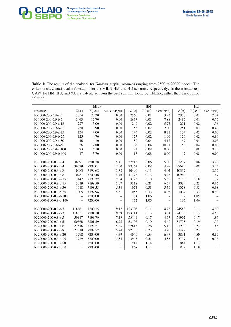
CPLEX was able to solve at the optimum, instances with 1000 nodes. For instances with 10000and 20000 nodes, memory problems only permit feasible solutions to be found. In the tables, whenthe optimal value for the instance is known, we refer to it as GAP. When CPLEX can not find theoptimal solution, we give the gap estimated by CPLEX (denoted as Est. Gap) and the gap betweenthe best known value found by CPLEX and that found by the heuristic (denoted as GAP*).

Table 1 shows that the exact algorithm leads to larger values for the gaps as the complexity ofthe instances increases. With respect to the heuristics HM and HU, it is clear that HU has a betterperformance than HM and the gap of solutions found by HU is always small.

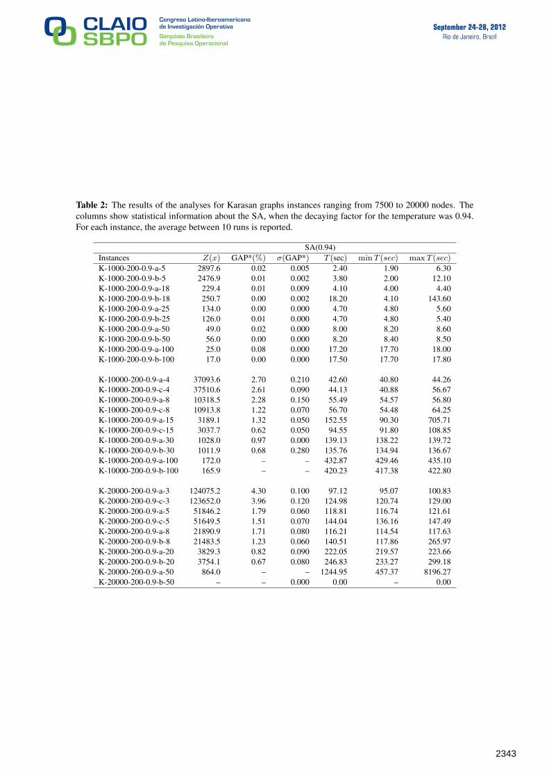
From Table 2 it is noted first that SA is able to obtain feasible solutions in no more than 22minutes for all instances. Only a single instance with 20000 nodes took 1245 seconds (on average)and the other solutions were obtained within 433 seconds or less. We observe that in most instancesSA was able to improve the solution given by the heuristic and all the instances achieved solutionswith small gaps with respect to the best solution given by CPLEX. For the most part, there is verylittle variation in both the running time and the quality of the solution when using SA. However,for two instances, one with 10000 nodes and the other with 20000 nodes, the running time had verysignificant differences.

For random networks CPLEX was able to optimally solve all the instances. Our results forrandom instances confirm the results commented in others papers. These classes of instances arenot complicated for exact algorithms. HU has better performance than HM and almost always findsan optimal solution. In two particular cases HM and HU only find good feasible solutions. In thesecases, SA was not be able to improve on the solution provided by HU.

6 Conclusions and Future Work

A novel neighbor generation method for a SA algorithm was proposed and used for solving theinterval data minmax regret path problem. The performance of this method was compared withthe performance of two known simple and effective heuristics for MMRCO problems; the optimalsolution (in most cases) was provided by CPLEX from a linear integer programming formulationknown for MMRP. Two classes of instances were considered for experimentation; random graphsand Karasan graphs. For random graphs, the optimal solutions were always obtained by CPLEX inreasonable times. The heuristic using the upper bound scenario outperforms that using the midpointscenario in this problem and almost always finds the optimal solutions.

For Karasan graphs, the optimal solution was always found by CPLEX for instances with 1000nodes. All the instances with 10000 and 20000 nodes had estimated gaps between 2.07% and9.17% within the time limit. Also, in some cases CPLEX was not able to find the optimum becauseof memory overflow errors.

According to our experiments, there are many cases where the SA improves on the result ofthe HU and HM algorithm. In particular, in the case when the cardinality of the datasets is large.This is an important feature of our proposed SA algorithm, that is, it consistently improves on thebest of two basic heuristics for the broad range of Karasan instances we tested. This shows that themethod of perturbing the search space during the neighbor generation process in the SA algorithmis an effective means of generating better solutions than the two heuristic algorithms.

For future work, when using SA in Minmax regret problems, it would be ideal to considermore variety on some parameters when defining the test instances e.g., the parameter c. Also,the neighborhood scheme used here could be considered when using different metaheuristics, likeGenetic Algorithms, to solve Minmax Regret combinatorial optimization problems.

9

2340


References

Ahuja, R. K., Magnanti, T. L., and Orlin, J. B. (1993). Network flows: theory, algorithms, andapplications. Prentice Hall, Upper Saddle River, NJ.

Aissi, H., Bazgan, C., and Vanderpooten, D. (2009). Min-max and min-max regret versions ofcombinatorial optimization problems: A survey. European Journal of Operational Research,197(2):427–438.

Candia-Véjar, A., Alvarez-Miranda, E., and Maculan, N. (2011). Minmax regret combinatorialoptimization problems: an algorithmic perspective. RAIRO Op. Research, 45(2):101–129.

Conde, E. and Candia, A. (2007). Minimax regret spanning arborescences under uncertain costs.European Journal of Operational Research, 182(2):561–577.

Dijkstra, E. W. (1959). A note on two problems in connexion with graphs. Numerische Mathematik,1(1):269–271.

Dréo, J., Pétrowski, A., Siarry, P., and Taillard, E. (2006). Metaheuristics for Hard Optimization.Springer.

Karasan, O., Pinar, M., and Yaman, H. (2001). The robust shortest path problem with interval data.Technical report, Bilkent University.

Kasperski, A. (2008). Discrete Optimization with Interval Data, volume 228 of Studies in Fuzzinessand Soft Computing. Springer Berlin Heidelberg, Berlin, Heidelberg.

Kirkpatrick, S., Gelatt, C. D., and Vecchi, M. P. (1983). Optimization by simulated annealing.Science, 220(4598):671–680.

Kouvelis, P. and G., Y. (1997). Robust discrete optimization and its applications. Kluwer AcademicPublishers.

Luke, S. (2009). Essentials of Metaheuristics. Lulu. Available for free athttp://cs.gmu.edu/∼sean/book/metaheuristics/.

Montemanni, R., Barta, J., Mastrolilli, M., and Gambardella, L. M. (2007). The Robust TravelingSalesman Problem with Interval Data. Transportation Science, 41(3):366–381.

Montemanni, R. and Gambardella, L. M. (2004). An exact algorithm for the robust shortest pathproblem with interval data. Computers & Operations Research, 31(10):1667–1680.

Montemanni, R. and Gambardella, L. M. (2005). The robust shortest path problem with intervaldata via Benders decomposition. 4or, 3(4):315–328.

Nikulin, Y. (2007). Simulated annealing algorithm for the robust spanning tree problem. Journalof Heuristics, 14(4):391–402.

Pereira, J. and Averbakh, I. (2011a). Exact and heuristic algorithms for the interval data robustassignment problem. Computers & Operations Research, 38(8):1153–1163.

Pereira, J. and Averbakh, I. (2011b). The robust set covering problem with interval data. Annals ofOperations Research, pages 1–19. DOI: 10.1007/s10479-011-0876-5.

10

2341


Table 1: The results of the analyses for Karasan graphs instances ranging from 7500 to 20000 nodes. Thecolumns show statistical information for the MILP, HM and HU schemes, respectively. In these instances,GAP* for HM, HU, and SA are calculated from the best solution found by CPLEX, rather than the optimalsolution.

MILP HM HUInstances Z(x) T (sec) Est. GAP(%) Z(x) T (sec) GAP*(%) Z(x) T (sec) GAP*(%)K-1000-200-0.9-a-5 2854 23.30 0.00 2966 0.01 3.92 2918 0.01 2.24K-1000-200-0.9-b-5 2463 12.70 0.00 2657 0.01 7.88 2482 0.01 0.77K-1000-200-0.9-a-18 227 3.00 0.00 240 0.02 5.73 231 0.02 1.76K-1000-200-0.9-b-18 250 3.90 0.00 255 0.02 2.00 251 0.02 0.40K-1000-200-0.9-a-25 134 4.00 0.00 145 0.02 8.21 134 0.02 0.00K-1000-200-0.9-b-25 125 4.70 0.00 127 0.02 1.60 126 0.02 0.80K-1000-200-0.9-a-50 48 4.10 0.00 50 0.04 4.17 49 0.04 2.08K-1000-200-0.9-b-50 56 2.80 0.00 62 0.04 10.71 56 0.04 0.00K-1000-200-0.9-a-100 23 4.10 0.00 23 0.08 0.00 25 0.08 8.70K-1000-200-0.9-b-100 17 3.70 0.00 17 0.08 0.00 17 0.08 0.00

K-10000-200-0.9-a-4 36091 7201.78 5.41 37912 0.06 5.05 37277 0.06 3.29K-10000-200-0.9-c-4 36539 7202.01 7.00 38362 0.08 4.99 37685 0.08 3.14K-10000-200-0.9-a-8 10083 7199.62 3.38 10490 0.11 4.04 10337 0.11 2.52K-10000-200-0.9-c-8 10781 7200.46 4.46 11372 0.13 5.48 10940 0.13 1.47K-10000-200-0.9-a-15 3147 7199.32 2.64 3322 0.18 5.56 3190 0.18 1.37K-10000-200-0.9-c-15 3019 7198.59 2.07 3218 0.21 6.59 3039 0.23 0.66K-10000-200-0.9-a-30 1018 7198.53 5.34 1074 0.33 5.50 1028 0.33 0.98K-10000-200-0.9-b-30 1005 7197.98 5.31 1055 0.33 4.98 1014 0.33 0.90K-10000-200-0.9-a-100 – 7200.00 – 184 1.06 – 172 1.05 –K-10000-200-0.9-b-100 – 7200.00 – 172 1.05 – 166 1.06 –

K-20000-200-0.9-a-3 118661 7200.15 9.17 123705 0.11 4.25 124588 0.11 4.99K-20000-200-0.9-c-3 118751 7201.10 9.39 123314 0.13 3.84 124170 0.13 4.56K-20000-200-0.9-a-5 50917 7199.79 7.19 53141 0.17 4.37 51902 0.17 1.93K-20000-200-0.9-c-5 50868 7201.39 6.75 53107 0.19 4.40 51735 0.19 1.70K-20000-200-0.9-a-8 21516 7199.21 5.36 22613 0.26 5.10 21913 0.24 1.85K-20000-200-0.9-c-8 21219 7202.52 5.24 22270 0.23 4.95 21499 0.23 1.32K-20000-200-0.9-a-20 3798 7200.00 4.39 4040 0.53 6.37 3831 0.50 0.87K-20000-200-0.9-b-20 3729 7200.00 5.34 3947 0.51 5.85 3757 0.51 0.75K-20000-200-0.9-a-50 – 7200.00 – 917 1.14 – 864 1.13 –K-20000-200-0.9-b-50 – 7200.00 – 868 1.14 – 838 1.19 –

11

2342


Table 2: The results of the analyses for Karasan graphs instances ranging from 7500 to 20000 nodes. Thecolumns show statistical information about the SA, when the decaying factor for the temperature was 0.94.For each instance, the average between 10 runs is reported.

SA(0.94)Instances Z(x) GAP*(%) σ(GAP*) T (sec) minT (sec) maxT (sec)

K-1000-200-0.9-a-5 2897.6 0.02 0.005 2.40 1.90 6.30K-1000-200-0.9-b-5 2476.9 0.01 0.002 3.80 2.00 12.10K-1000-200-0.9-a-18 229.4 0.01 0.009 4.10 4.00 4.40K-1000-200-0.9-b-18 250.7 0.00 0.002 18.20 4.10 143.60K-1000-200-0.9-a-25 134.0 0.00 0.000 4.70 4.80 5.60K-1000-200-0.9-b-25 126.0 0.01 0.000 4.70 4.80 5.40K-1000-200-0.9-a-50 49.0 0.02 0.000 8.00 8.20 8.60K-1000-200-0.9-b-50 56.0 0.00 0.000 8.20 8.40 8.50K-1000-200-0.9-a-100 25.0 0.08 0.000 17.20 17.70 18.00K-1000-200-0.9-b-100 17.0 0.00 0.000 17.50 17.70 17.80

K-10000-200-0.9-a-4 37093.6 2.70 0.210 42.60 40.80 44.26K-10000-200-0.9-c-4 37510.6 2.61 0.090 44.13 40.88 56.67K-10000-200-0.9-a-8 10318.5 2.28 0.150 55.49 54.57 56.80K-10000-200-0.9-c-8 10913.8 1.22 0.070 56.70 54.48 64.25K-10000-200-0.9-a-15 3189.1 1.32 0.050 152.55 90.30 705.71K-10000-200-0.9-c-15 3037.7 0.62 0.050 94.55 91.80 108.85K-10000-200-0.9-a-30 1028.0 0.97 0.000 139.13 138.22 139.72K-10000-200-0.9-b-30 1011.9 0.68 0.280 135.76 134.94 136.67K-10000-200-0.9-a-100 172.0 – – 432.87 429.46 435.10K-10000-200-0.9-b-100 165.9 – – 420.23 417.38 422.80

K-20000-200-0.9-a-3 124075.2 4.30 0.100 97.12 95.07 100.83K-20000-200-0.9-c-3 123652.0 3.96 0.120 124.98 120.74 129.00K-20000-200-0.9-a-5 51846.2 1.79 0.060 118.81 116.74 121.61K-20000-200-0.9-c-5 51649.5 1.51 0.070 144.04 136.16 147.49K-20000-200-0.9-a-8 21890.9 1.71 0.080 116.21 114.54 117.63K-20000-200-0.9-b-8 21483.5 1.23 0.060 140.51 117.86 265.97K-20000-200-0.9-a-20 3829.3 0.82 0.090 222.05 219.57 223.66K-20000-200-0.9-b-20 3754.1 0.67 0.080 246.83 233.27 299.18K-20000-200-0.9-a-50 864.0 – – 1244.95 457.37 8196.27K-20000-200-0.9-b-50 – – 0.000 0.00 – 0.00

12

2343

a simulated annealing approach for the minmax regret path ... · averbakh (pereira and averbakh,...

Documents