This content has been downloaded from IOPscience. Please scroll down to see the full text.

Download details:

IP Address: 132.236.27.111

This content was downloaded on 27/05/2014 at 10:32

Please note that terms and conditions apply.

A series study of a mixed-spin ferrimagnetic Ising model

View the table of contents for this issue, or go to the journal homepage for more

2006 J. Phys.: Condens. Matter 18 10931

(http://iopscience.iop.org/0953-8984/18/48/020)

Home Search Collections Journals About Contact us My IOPscience

INSTITUTE OF PHYSICS PUBLISHING JOURNAL OF PHYSICS: CONDENSED MATTER

J. Phys.: Condens. Matter 18 (2006) 10931–10942 doi:10.1088/0953-8984/18/48/020

A series study of a mixed-spin S = (12, 1) ferrimagnetic

Ising model

J Oitmaa1,3 and I G Enting2

1 School of Physics, The University of New South Wales, Sydney, NSW 2052, Australia2 MASCOS, 139 Barry Street, The University of Melbourne, Vic 3010, Australia

Received 12 September 2006, in final form 26 October 2006Published 17 November 2006Online at stacks.iop.org/JPhysCM/18/10931

AbstractWe use both high- and low-temperature series expansions to investigate thephase diagram of a ferrimagnetic mixed-spin S = (1/2, 1) Ising model onthe square lattice, including an on-site anisotropy term on the S = 1 sites.Evidence is found for a first-order transition for large negative anisotropy, andhence for the existence of a tricritical point. The model, with nearest neighbourinteractions only, does not appear to have a ferrimagnetic compensation point.

1. Introduction

Mixed-spin Ising models have been studied for some time as simple models of ferrimagnetism,and there has been renewed interest recently in connection with compensation points. Theseare temperatures, below the critical point, where the sublattice magnetizations exactly cancel,with zero total moment. As the temperature is tuned through such a point the total momentchanges sign. In this context Ising models have the virtue of being exactly solvable in specialcases [1] or solvable to high numerical precision by Monte Carlo [2, 3] or other methods.

The present paper uses high- and low-temperature series expansions to study a particularmixed-spin model. A bipartite square lattice has S = 1

2 spins on one sublattice (denoted A)and S = 1 spins on the other (denoted B), with nearest neighbour interactions and a single-ionanisotropy term on the S = 1 sites. The Hamiltonian of our model is

H = −J∑

〈i j〉σi S j − h A

∑

i∈A

σi − hB

∑

j∈B

S j − D∑

j∈B

S2j (1)

where σi = ±1, Sj = 1, 0,−1, h A and hB are fields on the two species and D is the anisotropy.Note that we choose σi = ±1 rather than ± 1

2 as done by some other authors, This simplyamounts to a rescaling of the exchange constant J . Note also that we have written H in theform of a ferromagnet (J > 0) but this is equivalent to a ferrimagnet by a simple spin reversalon either sublattice.

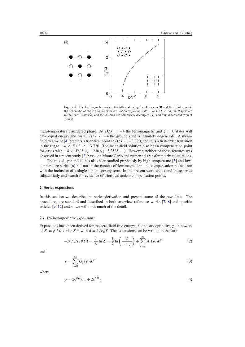
The model, and a schematic phase diagram, are shown in figure 1. For D/J > −4there will be a transition line separating the low-temperature ferromagnetic phase from the

3 Author to whom any correspondence should be addressed.

0953-8984/06/4810931+12$30.00 © 2006 IOP Publishing Ltd Printed in the UK 10931

10932 J Oitmaa and I G Enting

(a) (b)

D/J

k BT

/J

-6 -4 -2 0 20

2

Figure 1. The ferrimagnetic model: (a) lattice showing the A sites as • and the B sites as ◦.(b) Schematic of phase diagram with illustration of ground states. For D/J < −4, the B spins arein the ‘zero’ state (◦) and the A spins are completely decoupled (•), and thus disordered even atT = 0.

high-temperature disordered phase. At D/J = −4 the ferromagnetic and S = 0 states willhave equal energy and for all D/J < −4 the ground state is infinitely degenerate. A mean-field treatment [4] predicts a tricritical point at D/J = −3.720, and thus a first-order transitionin the range −4 < D/J < −3.720. The mean-field solution also has a compensation pointfor cases with −4 < D/J � −2 ln 6 (−3.3535 . . .). However, neither of these features wasobserved in a recent study [2] based on Monte Carlo and numerical transfer matrix calculations.

The mixed-spin model has also been studied previously by high-temperature [5] and low-temperature series [6] but not in the context of ferrimagnetism and compensation points, norwith the inclusion of a single-ion anisotropy term. In the present work we extend these seriessubstantially and search for evidence of tricritical and/or compensation points.

2. Series expansions

In this section we describe the series derivation and present some of the raw data. Theprocedures are standard and described in both overview reference works [7, 8] and specificarticles [9–12] and so we will omit much of the detail.

2.1. High-temperature expansions

Expansions have been derived for the zero-field free energy, f , and susceptibility, χ , in powersof K = β J to order K 16 with β = 1/kBT . The expansions can be written in the form

−β f (H, βD) = 1

Nln Z = 1

2ln

(2

1 − p

)+

∞∑

r=2

Ar (p)K r (2)

and

χ =∞∑

r=0

Gg(p)K r (3)

where

p = 2eβD/(1 + 2eβD) (4)

Series study of mixed-spin ferromagnetic Ising model 10933

and Ar (p) and Gr (p) are polynomials in p. These polynomials are given in appendix A. Wenote that earlier series work [5] gives the coefficients Ar to order 10 and Gr to order 7 only forthe case p = 2

3 (D = 0). Our extended results confirm these.A few technical comments are in order. The free energy series was derived by the direct

method involving both connected and disconnected graphs with single and double bonds. Forp = 1 (D = ∞) the S = 0 states are suppressed and the series should reduce to the knownspin- 1

2 Ising series [9]. This provides a partial check on the correctness of our results. Thesusceptibility series was obtained using the ‘vertex-renormalized linked-cluster’ method [10].To obtain the susceptibility with respect to a uniform external field h we write the specificfields as h A = m Ah and hB = m Bh where m A = 1

2 and m B = 1 are the relative magneticmoments. In this case, the p = 1 limit is not exactly the known spin- 1

2 susceptibility series,because of the different moments, but odd and even coefficients in the expansion of the mixed-spin susceptibility are related to the corresponding coefficients in the spin- 1

2 case by factors of2m A m B = 1 and m2

A + m2B = 5

4 , respectively. This has provided an additional check on ourseries. We have taken every care to avoid errors, but even with these checks the possibility ofsmall errors in the high-order coefficients cannot be excluded.

In section 3 of the paper, we will use the susceptibility series to obtain the locus of theline of critical points of the model and use the free energy series to search for evidence of afirst-order transition, using ‘free energy matching’.

2.2. Low-temperature expansions

Expansions have been derived for the zero-field free energy and sublattice magnetizations,MA = 1

2 〈σ 〉 and MB = 〈S〉, in powers of the variable u = exp(−2J/kBT ) = exp(−2K ). Theexpansions take the form

−β f (u, βD) = 4β J + βD +∞∑

r=2

ψr (y) ur (5)

2MA = 1 −∞∑

r=4

μ[A]r (y) ur (6)

MB = 1 −∞∑

r=4

μ[B]r (y) ur (7)

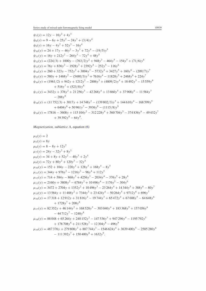
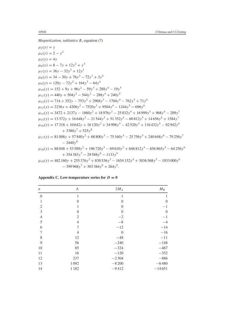
where y = exp(−βD). The quantities ψr (y), μ[A]r (y) and μ[B]

r (y) are polynomials in y andare given in appendix B to order r = 19. Thus the resulting series can be obtained to order u19

for any fixed value of βD.These series were derived using the method of partial generating functions (PGF) [7, 11]

where each PGF corresponds to a fixed number of spin excitations on the A sublattice. Bowersand Yousif [6] have shown that these can be obtained from the corresponding PGFs for thepure spin- 1

2 problem. Using the published PGFs to F7 [11] and augmenting these with thelower-order (in u) contributions to F8, F9 and F10 allows a ‘temperature grouping’ to order u19

to be computed. A check is available for the case y = 1 (D = 0) as discussed below. Theseries will be used in section 3 to explore the region D/J � −3 where the most interestingphysics is expected.

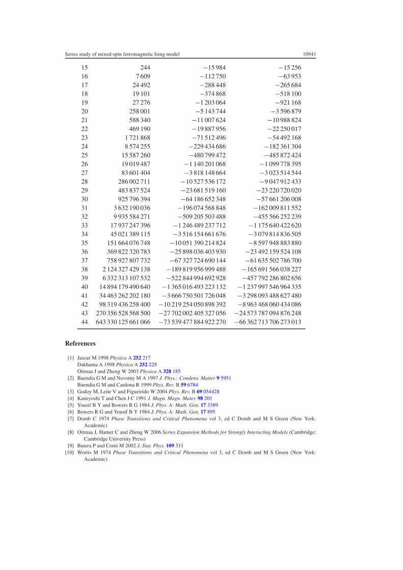
An alternative, usually more powerful, method of obtaining low-temperature seriesexpansions, particularly in two dimensions, is the finite lattice method (FLM) [12]. We haveadapted this method to the mixed-spin problem and obtained series for Z (rather than for ln Z )and the sublattice magnetizations for the case D = 0. The FLM combinatorics for treating

10934 J Oitmaa and I G Enting

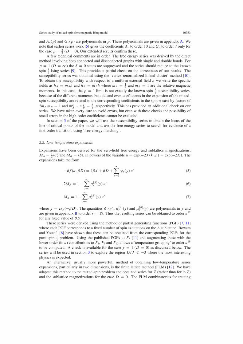
Table 1. Estimates of critical temperature kTc/J for various D/J from analysis of high-temperature susceptibility series. The values of Kc for χ and M are from high-temperaturesusceptibility series and low-temperature magnetization series, respectively.

βD Kc (χ ) Kc (M) kTc/J D/J

0.940 0.4713(1) — 2.122(1) 1.9440.488 0.4870(3) — 2.053(1) 1.0020 0.5120(5) 0.5199 1.953(2) 0

−0.553 0.5535(10) — 1.807(3) −0.999−0.765 0.5735(10) 0.5725 1.744(3) −1.334−1.260 0.630(1) 0.6285 1.587(3) −2.000−1.935 0.729(2) — 1.372(3) −2.654−2.450 0.815(5) — 1.227(6) −3.006−5.000 1.36(1) — 0.735(5) −3.67

sublattices is a slightly simplified case of that described for the checkerboard lattice [17]. Theseries are given in appendix C. These data provide a check on the shorter general series for thecase y = 1.

It is possible to include the single-ion anisotropy in FLM calculations. However, issuesof numerical precision and storage requirements mean that this is most easily done for single-variable series defined by y = un/m so that D/J = 2n/m where n = 4k − 2m and k andm are small integers. We have derived series (of varying length) for a number of choices ofn/m. These series are valuable, in conjunction with the high-temperature susceptibility, inlocating the critical line. Magnetization series for D/J = 0,−4/3,−2 were used to obtainestimates of the critical temperature, given in table 1. We have also calculated series for thecases D/J = 4, 8, 16. However, it has not been possible to explore the region D/J � −3 inthis way.

3. Results

We now turn to the results obtained by analysis of the various series.

3.1. The critical line

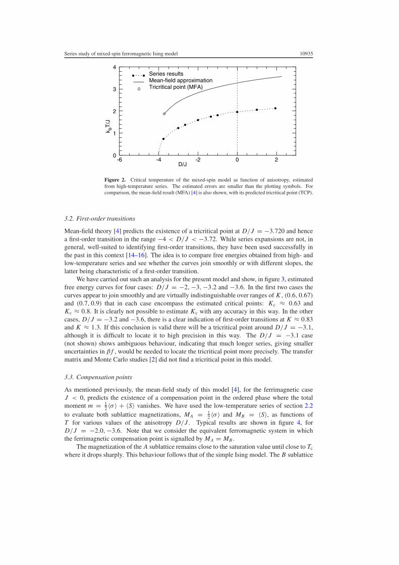
As shown in the schematic phase diagram (figure 1(b)), the model will have a line of criticalpoints in the (T, D) plane. Critical temperatures are usually obtained most precisely fromanalysis of the high-temperature susceptibility series. We choose fixed values of βD, obtainthe critical point Kc from a standard Pade approximant analysis [13] of both logarithmicderivative series and the series for χ4/7 which should have a simple pole, and obtain thecorresponding values of D/J as βD/Kc. In table 1, we give estimates of kBT/J . The quoteduncertainties are, as usual, confidence limits based on consistency and apparent convergenceamong a range of approximants. The resulting critical curve is shown in figure 2. ForβD � −3.0 the susceptibility series becomes more and more irregular and the analysis moreproblematic. This is due to the presence of interfering singularities and we are unable tocontinue the line to D/J = −4 where Tc = 0. If the transition in this region becomesfirst-order, as we argue below, the high-temperature susceptibility series will not in any casediverge at the true transition temperature but at a spinodal line within the ordered phase. Thecritical line obtained in the present study agrees well with earlier results from a transfer matrixapproach [2] and lies substantially below the mean-field curve [4] which is shown in figure 2for comparison.

Series study of mixed-spin ferromagnetic Ising model 10935

D/J

k BT

/J

-6 -4 -2 0 20

1

2

3

4Series resultsMean-field approximationTricritical point (MFA)

Figure 2. Critical temperature of the mixed-spin model as function of anisotropy, estimatedfrom high-temperature series. The estimated errors are smaller than the plotting symbols. Forcomparison, the mean-field result (MFA) [4] is also shown, with its predicted tricritical point (TCP).

3.2. First-order transitions

Mean-field theory [4] predicts the existence of a tricritical point at D/J = −3.720 and hencea first-order transition in the range −4 < D/J < −3.72. While series expansions are not, ingeneral, well-suited to identifying first-order transitions, they have been used successfully inthe past in this context [14–16]. The idea is to compare free energies obtained from high- andlow-temperature series and see whether the curves join smoothly or with different slopes, thelatter being characteristic of a first-order transition.

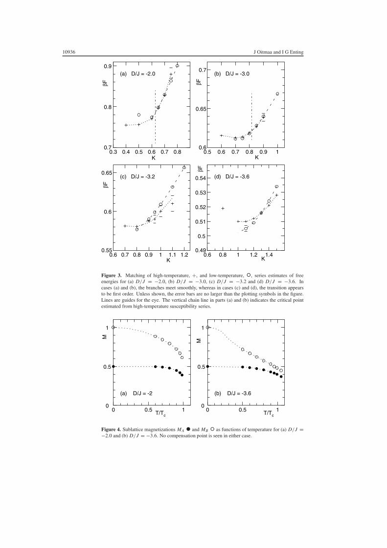
We have carried out such an analysis for the present model and show, in figure 3, estimatedfree energy curves for four cases: D/J = −2,−3,−3.2 and −3.6. In the first two cases thecurves appear to join smoothly and are virtually indistinguishable over ranges of K , (0.6, 0.67)and (0.7, 0.9) that in each case encompass the estimated critical points: Kc ≈ 0.63 andKc ≈ 0.8. It is clearly not possible to estimate Kc with any accuracy in this way. In the othercases, D/J = −3.2 and −3.6, there is a clear indication of first-order transitions at K ≈ 0.83and K ≈ 1.3. If this conclusion is valid there will be a tricritical point around D/J = −3.1,although it is difficult to locate it to high precision in this way. The D/J = −3.1 case(not shown) shows ambiguous behaviour, indicating that much longer series, giving smalleruncertainties in β f , would be needed to locate the tricritical point more precisely. The transfermatrix and Monte Carlo studies [2] did not find a tricritical point in this model.

3.3. Compensation points

As mentioned previously, the mean-field study of this model [4], for the ferrimagnetic caseJ < 0, predicts the existence of a compensation point in the ordered phase where the totalmoment m = 1

2 〈σ 〉 + 〈S〉 vanishes. We have used the low-temperature series of section 2.2to evaluate both sublattice magnetizations, MA = 1

2 〈σ 〉 and MB = 〈S〉, as functions ofT for various values of the anisotropy D/J . Typical results are shown in figure 4, forD/J = −2.0,−3.6. Note that we consider the equivalent ferromagnetic system in whichthe ferrimagnetic compensation point is signalled by MA = MB .

The magnetization of the A sublattice remains close to the saturation value until close to Tc

where it drops sharply. This behaviour follows that of the simple Ising model. The B sublattice

10936 J Oitmaa and I G Enting

(a) D/J = -2.0 (b) D/J = -3.0

(c) D/J = -3.2 (d) D/J = -3.6

K

βF

0.3 0.4 0.5 0.6 0.7 0.80.7

0.8

0.9

0.6 0.7 0.8 0.9 1 1.1 1.20.55

0.6

0.65

K

βF

0.5 0.6 0.7 0.8 0.9 10.6

0.65

0.7

K

βF

K

βF

0.6 0.8 1 1.2 1.40.49

0.5

0.51

0.52

0.53

0.54

Figure 3. Matching of high-temperature, +, and low-temperature, ◦, series estimates of freeenergies for (a) D/J = −2.0, (b) D/J = −3.0, (c) D/J = −3.2 and (d) D/J = −3.6. Incases (a) and (b), the branches meet smoothly, whereas in cases (c) and (d), the transition appearsto be first order. Unless shown, the error bars are no larger than the plotting symbols in the figure.Lines are guides for the eye. The vertical chain line in parts (a) and (b) indicates the critical pointestimated from high-temperature susceptibility series.

(a) D/J = -2 (b) D/J = -3.6

T/Tc

M

0 0.5 10

0.5

1

T/Tc

M

0 0.5 10

0.5

1

Figure 4. Sublattice magnetizations MA • and MB ◦ as functions of temperature for (a) D/J =−2.0 and (b) D/J = −3.6. No compensation point is seen in either case.

Series study of mixed-spin ferromagnetic Ising model 10937

magnetization, on the other hand, has a more complex temperature dependence and develops apoint of inflection for D/J approaching −4. Physically this is due to an increasing populationof the S = 0 state with increasing temperature and is the precursor to a compensation point(where MB would fall below MA). However, we find no compensation point, down to at leastD/J = −3.9.

4. Conclusions

We have used high- and low-temperature series expansions to investigate a mixed-spin S =( 1

2 , 1) Ising model with nearest neighbour interactions on the square lattice. A single-ionanisotropy term is included in the S = 1 sublattice. Our main motivation has been to search forthe existence of a tricritical point and/or compensation point, both of which are predicted bymean-field theory [4], but neither of which was found by a more reliable Monte Carlo/transfermatrix study [2]. In the process we have substantially extended the series for this model.

Although we find no compensation point, the magnetization of the S = 1 sublattice showsan anomalous temperature dependence for large negative anisotropy D, which if magnifiedwould lead to a compensation point. Rather surprisingly, we do find evidence for a first-order transition at large negative D and hence for a tricritical point that is not seen in previouswork [2]. This suggests that further study of the model is warranted.

The previous study [2] found that inclusion of a next-nearest neighbour interaction betweenthe S = 1

2 spins did yield a compensation point. Such an interaction will stiffen the order onthe A sublattice to higher temperatures. We have not included such an interaction in our serieswork although it could be done with some effort.

Series expansion methods have not, to our knowledge, been used previously in lookingfor compensation points in ferrimagnetic models. However, as we demonstrate here, they canpotentially be a powerful approach. Provided that reasonably long magnetization series canbe derived, the resulting analysis can be quite precise, as the compensation point, unlike thecritical point, is not a singularity.

Acknowledgments

Jaan Oitmaa thanks the Australian Research Council for support. The ARC Center ofExcellence for Mathematics and Statistics of Complex Systems (MASCOS) is funded by theAustralian Research Council. Ian Enting’s fellowship at MASCOS is supported in part byCSIRO.

Appendix A. High-temperature polynomials

Free energy equation (2)

A2(p) = p

A4(p) = (5/6)p

A6(p) = (17/45)p + p2 − (2/3)p3

A8(p) = (13/126)p + (7/4)p2 − (5/3)p3 + (3/2)p4

A10(p) = (257/14 175)p + (22/15)p2 − (29/45)p3 + 4p4 − (4/5)p5

A12(p) = (205/93 555)p + (1453/1890)p2 + (2153/1134)p3 + (28/5)p4 + (8/3)p5 + p6

A14(p) = (8194/42 567 525)p + (1406/4995)p2 + (9383/2835)p3 + (4635/567)p4

+ (254/15)p5 + 8p6 + (8/7)p7

10938 J Oitmaa and I G Enting

A16(p) = (3277/255 405 150)p + (15 949/207 900)p2 + (177 043/62 370)p3

+ (161 513/12 600)p4 + (12 449/315)p5 + (869/15)p6 + (14/3)p7

+ (45/4)p8.

Susceptibility equation (3)

G0(p) = (1/8)+ (1/2)p

G1(p) = 2p

G2(p) = (5/2)p + 5p2

G3(p) = (10/3)p + 14p2

G4(p) = (17/6)p + (86/3)p2 + 26p3

G5(p) = (34/15)p + 48p2 + 70p3

G6(p) = (13/9)p + (1075/18)p2 + (1205/6)p3 + 120p4

G7(p) = (52/63)p + (1064/15)p2 + (1114/3)p3 + 326p4

G8(p) = (257/630)p + (20 921/315)p2 + (6227/10)p3 + (2303/2)p4 + 540p5

G9(p) = (514/2835)p + (1648/27)p2 + (7900/9)p3 + (6928/3)p4 + 1434p5

G10(p) = (41/567)p + (262 741/5670)p2 + (412 487/378)p3 + (28 385/6)p4

+ (12 133/2)p5 + 2328p6

G11(p) = (164/6237)p + (18 232/525)p2 + (167 818/135)p3 + (112 784/15)p4

+ 12698p5 + 6164p6

G12(p) = (4097/467 775)p + (10 387 387/467 775)p2 + (35 464 649/28 350)p3

+ (64 646 307/5670)p4 + (91 642/3)p5 + 30346p6 + 9724p7

G13(p) = (16 388/6081 075)p + (62 608/4455)p2 + (96 868/81)p3

+ (74 990 194/4995)p4 + (788 602/15)p5 + (196 214/3)p6 + 25 730p7

G14(p) = (6554/8513 505)p + (66 025 327/8513 505)p2 + (235 394/231)p3

+ (498 094/27)p4 + (1953 221/21)p5 + (361 211/2)p6 + (288 405/2)p7

+ 40392p8

G15(p) = (26 216/127 702 575)p + (18 455 024/4343 625)p2 + (130 902 236/155 925)p3

+ (98 021 494/4725)p4 + (42 746 416/315)p5 + (14 770 084/45)p6

+ (956 302/3)p7 + 106 216p8

G16(p) = (65 537/1277 025 750)p + (1315 330 466/638 512 875)p2

+ (10 192 275 347/16 372 125)p3 + (160 684 229/7425)p4

+ (122 425 943/630)p5 + (138 933 001/210)p6 + (14 870 686/15)p7

+ 668 719p8 + 164 358p9.

Appendix B. Low-temperature polynomials

Free energy equation (5)

ψ2(y) = y

ψ4(y) = 2 − (1/2)y2

ψ5(y) = 4y

ψ6(y) = 4 − 5y + 6y2 + (1/3)y3

Series study of mixed-spin ferromagnetic Ising model 10939

ψ7(y) = 12y − 16y2 + 4y3

ψ8(y) = 9 − 6y + 25y2 − 24y3 + (3/4)y4

ψ9(y) = 16y − 4y2 + 52y3 − 16y4

ψ10(y) = 24 + 17y − 46y2 − 3y3 + 72y4 − (19/5)y5

ψ11(y) = 16y + 212y2 − 264y3 − 72y4 + 48y5

ψ12(y) = (224/3)+ 1000y − (763/2)y2 + 948y3 − 464y5 − 154y5 + (71/6)y6

ψ13(y) = 76y + 836y2 − 1928y3 + 2392y4 − 252y5 − 116y6

ψ14(y) = 260 + 323y − 752y2 + 3004y3 − 5732y4 + 3427y5 + 160y6 − (209/7)y7

ψ15(y) = 580y + 1468y2 − (5480/3)y3 + 7616y4 − 11828y5 + 2468y6 + 224y7

ψ16(y) = (1961/2)+ 942y + 1212y2 − 2886y3 + (4809/2)y4 + 18 492y5 − 15 559y6

+ 516y7 + (523/8)y8

ψ17(y) = 3432y + 376y2 + 21 256y3 − 42 268y4 + 13 860y5 + 37 908y6 − 11 584y7

− 288y8

ψ18(y) = (11 752/3)+ 3017y + 14 748y2 − (139 802/3)y3 + 144 610y4 − 168 599y5

+ 6404y6 + 50 961y7 − 3936y8 − (1115/8)y9

ψ19(y) = 17816 − 3608y + 115 104y2 − 312 228y4 + 560 704y5 − 374 836y6 − 49 432y7

+ 39 392y8 − 64y9.

Magnetization, sublattice A, equation (6)

μ4(y) = 2

μ5(y) = 8y

μ6(y) = 8 − 8y + 12y2

μ7(y) = 24y − 32y2 + 8y3

μ8(y) = 34 + 8y + 52y2 − 48y3 + 2y4

μ9(y) = 72y + 80y2 + 120y3 − 32y4

μ10(y) = 152 + 104y − 220y2 + 128y3 + 168y4 − 8y5

μ11(y) = 344y + 976y2 − 1216y3 − 96y4 + 112y5

μ12(y) = 714 + 584y − 868y2 + 4256y3 − 2034y4 − 376y5 + 28y6

μ13(y) = 2160y + 3808y2 − 6784y3 + 10 496y4 − 1176y5 − 304y6

μ14(y) = 3472 + 2704y + 1352y2 + 10 496y3 − 23 264y4 + 14 344y5 + 388y6 − 80y7

μ15(y) = 13 584y + 11 488y2 + 7344y3 + 23 424y4 − 50 264y5 + 9712y6 + 696y7

μ16(y) = 17 318 + 12 912y + 31 816y2 − 19 744y3 + 65 472y4 + 67 688y5 − 64 648y6

+ 1728y7 + 208y8

μ17(y) = 82 352y + 46 144y2 + 168 528y3 − 303 040y4 + 183 368y5 + 157 056y6

− 44 712y7 − 1248y8

μ18(y) = 88 048 + 65 264y + 240 152y2 − 147 536y3 + 947 296y4 − 1195 792y5

+ 178 708y6 + 211 528y7 − 12 304y8 − 496y9

μ19(y) = 487 376y + 279 808y2 + 887 744y3 − 1546 624y4 + 3639 400y5 − 2585 280y6

− 111 392y7 + 150 400y8 + 1632y9.

10940 J Oitmaa and I G Enting

Magnetization, sublattice B , equation (7)

μ2(y) = y

μ4(y) = 2 − y2

μ5(y) = 4y

μ6(y) = 8 − 7y + 12y2 + y3

μ7(y) = 36y − 32y2 + 12y3

μ8(y) = 34 − 30y + 76y2 − 72y3 + 3y4

μ9(y) = 120y − 72y2 + 164y3 − 64y4

μ10(y) = 152 + 9y + 96y2 − 59y3 + 288y4 − 19y5

μ11(y) = 440y + 504y2 − 544y3 − 288y4 + 240y5

μ12(y) = 714 + 352y − 753y2 + 2968y3 − 1704y4 − 762y5 + 71y6

μ13(y) = 2236y + 4200y2 − 7520y3 + 9504y4 − 1244y5 − 696y6

μ14(y) = 3472 + 2137y − 1860y2 + 18 976y3 − 25 832y4 + 16 999y5 + 968y6 − 209y7

μ15(y) = 13 372y + 16 648y2 − 21 544y3 + 51 352y4 − 60 812y5 + 14 656y6 + 1584y7

μ16(y) = 17 318 + 10 642y + 16 120y2 + 34 998y3 − 42 520y4 + 116 432y5 − 92 942y6

+ 3380y7 + 525y8

μ17(y) = 81 008y + 57 840y2 + 68 800y3 − 75 160y4 − 25 756y5 + 240 648y6 − 79 256y7

− 2440y8

μ18(y) = 88 048 + 53 589y2 + 196 720y3 − 69 610y3 + 646 812y4 − 656 865y5 − 64 256y6

+ 354 383y7 − 29 588y8 − 1133y9

μ19(y) = 482 160y + 255 376y2 + 830 536y3 − 1654 152y4 + 3036 568y5 − 1933 000y6

− 399 968y7 + 303 384y8 + 264y9.

Appendix C. Low-temperature series for D = 0

n � 2MA MB

0 1 1 11 0 0 02 1 0 −13 0 0 04 2 −2 −15 4 −8 −46 7 −12 −147 4 0 −168 12 −48 −119 56 −240 −148

10 85 −324 −46711 16 −120 −35212 237 −2 304 −88613 1 092 −8 200 −6 48014 1 182 −9 412 −14 651

Series study of mixed-spin ferromagnetic Ising model 10941

15 244 −15 984 −15 25616 7 609 −112 750 −63 95317 24 492 −288 448 −265 68418 19 101 −374 868 −518 10019 27 276 −1 203 064 −921 16820 258 001 −5 143 744 −3 596 87921 588 340 −11 007 624 −10 988 82422 469 190 −19 887 956 −22 250 01723 1 721 868 −71 512 496 −54 492 16824 8 574 255 −229 434 686 −182 361 30425 15 587 260 −480 799 472 −485 872 42426 19 019 487 −1 140 201 068 −1 099 778 39527 83 601 404 −3 818 148 664 −3 023 514 54428 286 002 711 −10 527 536 172 −9 047 912 43329 483 837 524 −23 681 519 160 −23 220 720 02030 925 796 394 −64 186 652 348 −57 661 206 00831 3 632 190 036 −196 074 568 848 −162 009 811 55232 9 935 584 271 −509 205 503 488 −455 566 252 23933 17 937 247 396 −1 246 489 237 712 −1 175 640 422 62034 45 021 389 115 −3 516 154 661 676 −3 079 814 836 50535 151 664 076 748 −10 051 390 214 824 −8 597 948 883 88036 369 822 320 783 −25 898 036 403 930 −23 492 159 524 10837 758 927 807 732 −67 327 724 690 144 −61 635 502 786 70038 2 124 327 429 138 −189 819 956 999 488 −165 691 566 038 22739 6 332 313 107 532 −522 844 994 692 928 −457 792 286 802 65640 14 894 179 490 640 −1 365 016 493 223 132 −1 237 997 546 964 33541 34 463 262 202 180 −3 666 750 501 726 048 −3 298 093 488 627 48042 98 319 436 258 400 −10 219 254 050 898 392 −8 963 468 060 434 08643 270 356 528 568 500 −27 702 002 405 327 056 −24 573 787 094 876 24844 643 330 125 661 066 −73 539 477 884 922 270 −66 362 713 706 273 013

References

[1] Jascur M 1998 Physica A 252 217Dakhama A 1998 Physica A 252 225Oitmaa J and Zheng W 2003 Physica A 328 185

[2] Buendia G M and Novotny M A 1997 J. Phys.: Condens. Matter 9 5951Buendia G M and Cardona R 1999 Phys. Rev. B 59 6784

[3] Godoy M, Leite V and Figueirido W 2004 Phys. Rev. B 69 054428[4] Kaneyoshi T and Chen J C 1991 J. Magn. Magn. Mater. 98 201[5] Yousif B Y and Bowers R G 1984 J. Phys. A: Math. Gen. 17 3389[6] Bowers R G and Yousif B Y 1984 J. Phys. A: Math. Gen. 17 895[7] Domb C 1974 Phase Transitions and Critical Phenomena vol 3, ed C Domb and M S Green (New York:

Academic)[8] Oitmaa J, Hamer C and Zheng W 2006 Series Expansion Methods for Strongly Interacting Models (Cambridge:

Cambridge University Press)[9] Butera P and Comi M 2002 J. Stat. Phys. 109 311

[10] Wortis M 1974 Phase Transitions and Critical Phenomena vol 3, ed C Domb and M S Green (New York:Academic)

10942 J Oitmaa and I G Enting

[11] Sykes M F, Gaunt D S, Mattingly S R, Essam J W and Elliott C J 1973 J. Math. Phys. 14 1066[12] Enting I G 1996 Nucl. Phys. B 47 180[13] Guttmann A J 1989 Phase Transitions and Critical Phenomena vol 13, ed C Domb and M S Green (New York:

Academic)[14] Saul D M, Wortis M and Stauffer D 1974 Phys. Rev. B 9 4964[15] Velgakis M J and Ferer M 1983 Phys. Rev. B 27 401[16] Briggs K, Enting I G and Guttmann A J 1994 J. Phys. A: Math. Gen. 27 1503[17] Enting I G 1987 J. Phys. A: Math. Gen. 20 L917