Earth-Science Reviews 134 (2014) 1–15

Contents lists available at ScienceDirect

Earth-Science Reviews

j ourna l homepage: www.e lsev ie r .com/ locate /earsc i rev

A review of Holocene solar-linked climatic variation on centennial tomillennial timescales: Physical processes, interpretative frameworks anda new multiple cross-wavelet transform algorithm

Willie Soon a,⁎, Victor M. Velasco Herrera b, Kandasamy Selvaraj c, Rita Traversi d, Ilya Usoskin e,Chen-Tung Arthur Chen f, Jiann-Yuh Lou g, Shuh-Ji Kao c, Robert M. Carter h, Valery Pipin i,Mirko Severi d, Silvia Becagli d

a Harvard-Smithsonian Center for Astrophysics, Cambridge, MA, USAb Instituto de Geofísica, Universidad Nacional Autónoma de México, Ciudad Universitaria, 04510 México D.F., Mexicoc State Key Laboratory of Marine Environmental Science, Xiamen University, Xiamen, Chinad Department of Chemistry “Ugo Schiff”, University of Florence, Sesto F.no, 50019 Florence, Italye Sodankylä Geophysical Observatory and Department of Physics, University of Oulu, 90014, Finlandf Institute of Marine Geology and Chemistry, National Sun Yat-sen University, Kaohsiung, Taiwang Department of Marine Sciences, Naval Academy, Kaohsiung, Taiwanh Institute of Public Affairs, Melbourne, Australiai Institute of Solar-Terrestrial Physics, Russian Academy of Sciences, 664033 Irkutsk, Russia

⁎ Corresponding author.E-mail address: wsoon@cfa.harvard.edu (W. Soon).

http://dx.doi.org/10.1016/j.earscirev.2014.03.0030012-8252/© 2014 Elsevier B.V. All rights reserved.

a b s t r a c t

a r t i c l e i n f o

Article history:Received 21 January 2014Accepted 13 March 2014Available online 21 March 2014

Keywords:Solar-climate variationsSolar activity proxiesWavelet transform

We report on the existence and nature of Holocene solar and climatic variations on centennial tomillennial time-scales. We introduce a new solar activity proxy, based on nitrate (NO3

−) concentration from the Talos Dome icecore, East Antarctica. We also use a new algorithm for computing multiple-cross wavelet spectra in time–fre-quency space that is generalized for multiple time series (beyond two). Our results provide a new interpretiveframework for relating Holocene solar activity variations on centennial tomillennial timescales to co-varying cli-mate proxies drawn from a widespread area around the globe. Climatic proxies used represent variation in theNorth Atlantic Ocean, Western Pacific Warm Pool, Southern Ocean and the East Asian monsoon regions. Ourwavelet analysis identifies fundamental solar modes at 2300-yr (Hallstattzeit), 1000-yr (Eddy), and 500-yr(unnamed) periodicities, leaves open the possibility that the 1500–1800-yr cycle may either be fundamentalor derived, and identifies intermediary derived cycles at 700-yr and 300-yr that may mark rectified responsesof the Atlantic thermohaline circulation to external solar modulation and pacing. Dating uncertainties suggestthat the 1500-yr and 1800-yr cycles described in the literature may represent either the same or two separatecycles, but in either case, and irrespective too of whether it is a fundamental or derived mode in the sense ofDima and Lohmann (2009), the 1500–1800-yr periodicity is widely represented in a large number ofpaleoclimate proxy records. It is obviously premature to reject possible links between changing solar activity atthese multiple scales and the variations that are commonly observed in paleoclimatic records.

© 2014 Elsevier B.V. All rights reserved.

Contents

1. Introduction . . . . . . . . . . . . . . . . . . . . . . . . . . . . . . . . . . . . . . . . . . . . . . . . . . . . . . . . . . . . . . . 22. Methods and choice of data series . . . . . . . . . . . . . . . . . . . . . . . . . . . . . . . . . . . . . . . . . . . . . . . . . . . . . 3

2.1. Three Solar Activity Proxies: Nitrate Talos Dome Ice Core (TALDICE), solar modulation parameter from 10Be and 14C . . . . . . . . . . . . 32.2. Choice of Holocene paleoclimatic time series from regions of the East Asian Monsoon, North Atlantic Ocean, Western Pacific Warm Pool and

Southern Ocean . . . . . . . . . . . . . . . . . . . . . . . . . . . . . . . . . . . . . . . . . . . . . . . . . . . . . . . . . . 52.2.1. Relative Gray Index (RGI) time series (Retreat Lake, Taiwan) . . . . . . . . . . . . . . . . . . . . . . . . . . . . . . . . . 52.2.2. Total Organic Carbon (TOC) time series (Okinawa Trough) . . . . . . . . . . . . . . . . . . . . . . . . . . . . . . . . . . 5

2 W. Soon et al. / Earth-Science Reviews 134 (2014) 1–15

2.2.3. Other time series . . . . . . . . . . . . . . . . . . . . . . . . . . . . . . . . . . . . . . . . . . . . . . . . . . . . . 52.2.4. Multiple-Cross-wavelet for time-frequency analysis with multiple time series . . . . . . . . . . . . . . . . . . . . . . . . . . 5

3. Results and discussion . . . . . . . . . . . . . . . . . . . . . . . . . . . . . . . . . . . . . . . . . . . . . . . . . . . . . . . . . . 63.1. Wavelet spectra of three solar proxies . . . . . . . . . . . . . . . . . . . . . . . . . . . . . . . . . . . . . . . . . . . . . . . . 63.2. Wavelet spectra of individual paleoclimatic data-series . . . . . . . . . . . . . . . . . . . . . . . . . . . . . . . . . . . . . . . . 83.3. Solar-related variability on centennial and millennial scales . . . . . . . . . . . . . . . . . . . . . . . . . . . . . . . . . . . . . . 9

4. Conclusions . . . . . . . . . . . . . . . . . . . . . . . . . . . . . . . . . . . . . . . . . . . . . . . . . . . . . . . . . . . . . . . 11Acknowledgements . . . . . . . . . . . . . . . . . . . . . . . . . . . . . . . . . . . . . . . . . . . . . . . . . . . . . . . . . . . . . . 11Appendix A. A new algorithm for multiple-cross-wavelet analysis with multiple time series . . . . . . . . . . . . . . . . . . . . . . . . . . . . 11References . . . . . . . . . . . . . . . . . . . . . . . . . . . . . . . . . . . . . . . . . . . . . . . . . . . . . . . . . . . . . . . . . . 13

1. Introduction

In 1973, Denton and Karlen published a pioneering study of glacierexpansion and contraction activity and associated tree-line fluctuationsduring the Holocene. Since then, numerous other paleoclimatic proxystudies have documented a rich pattern of Holocene climate variationand oscillation on multiple timescales. Our use of the terminology“centennial to millennial”1 in description of such variability followsthe order-of-magnitude tradition in geological literature, whereby theterms encompass several hundreds to several thousands of years.

Climatic rhythmicities2 previously identified in proxy studies includethe solar 50–100 year Gleissberg–Yoshimura cycle, a distinct 120-year cycle, the 200 year solar deVries–Suess cycle, the millennial Eddycycle (see Kanda, 1933 for an earlier speculation of this scale identifiedbased on ancient records of sunspots and auroras) and the bi-millennialHallstattzeit rhythm. We recognize the Hallstattzeit signature in thispaper at a periodicity of 2200–2400 years, which is consistent with itsformer identification at timescales of “~2000 year” by Obrochta et al.(2012), and of “~2400 year” by Vasiliev and Dergachev (2002) and“2500 year” by Debret et al. (2009) and Dima and Lohmann (2009).We also study other apparently derived climate modes on multi-centennial and millennial timescales include the well known 1500-year cycle as those proposed recently in Dima and Lohmann (2009).

Mayewski et al. (2004),Wanner et al. (2008) andDebret et al. (2009)have shown that the amplitudes of these centennial tomillennial climatevariations are quite large, generally accounting for between 10 and 30%of the total variance of a given paleo-time series. Mayewski et al.(1997) report that 40% of the variance of both the residual 14C and thepolar circulation index derived from the Greenland Ice Sheet Project 2(GISP2) Holocene glacio-chemical time series can be explained by justthe three bandpass-combined components of 2300 + 1450 + 512 yearvariability (see Fig. 9 of their paper).

Throughout this paper, we refer to 1500-yr or 1800-yr rhythms in-terchangeably because the underlying solar and climatic proxy recordsso far described do not have sufficient resolution to discriminate accu-rately between them. But we do consider the 1500-yr or 1800-yrsolar-climatic rhythm to be statistically different from those of 1000-yrand Hallstattzeit period of 2200–2300-yr and hence a distinction usefulfor physical interpretation.

An important reason for studyingmillennial scale variation (ormoregenerally any other repeating rhythmic timescale) is the possible use ofthe signals for diagnosing and contrasting between the competing

1 This term refers to orders of magnitude, i.e. to century-scale or millennial-scale, fol-lowing an established usage in parts of the literature.

2 We note that we have adopted and used phrases like “periodicities”, “cyclicities”, “os-cillations”, “timescales” and “rhythmicities” throughout the paper in the loose limit andconstraint of our wavelet time–frequency analysis. Such use of course contrasts with thestrict periodicity as often used and interpreted in the traditional Fourier transform sense.But we find that our usages stick more closely to the current state of our understanding ofclimate variations over the Holocene, rather than pretending any precise knowledge ordefinition of climate and its variations.We refer those readers interested in the rather poorstate of development of climate theory in this regard to Essex (2011) and Essex (2013).

physical processes that may have caused them. This was highlightedin the recent study by Konecky et al. (2013). Those authors showed ev-idence for the persistence of a millennial-scale intensification of therainfall in southwestern Indonesia, through their precipitation proxy,δDwax, from Lake Lading, East Java, and suggested that periods of higherrainfall were connected to the strengthening of the tropical PacificWalker circulation. In contrast, if the precipitation signals were to becontrolled by the migrations of Intertropical Convergence Zone (ITCZ)on multidecadal timescales, the authors suggested that they shouldhave seen a drying tendency rather than seeing the rainfall increasepersisting into the 20th century.

In seeking to better understand centennial to millennial solar andclimatic cyclicities, we have deliberately restricted our study to Holo-cene time-series. In this way, we avoid the complexity of the ocean-atmosphere interactionswith large ice-sheets that are known to be rep-resented by the abrupt, warming–cooling Dansgaard–Oeschger eventsand their associated Heinrich events of iceberg discharges during theLate Pleistocene and earlier glacial periods. It is probable that the broad-band 1600-year pacing of the large and abrupt 8–16 °C warming, andthe roughly equivalent 45 m of sea level rise that occurred duringDansgaard–Oeschger events (Schulz et al., 1999; Schulz, 2002; Pisiaset al., 2010; Petersen et al., 2013), involve a different set of physicalprocesses3 than those that were operating during the Holocene. In addi-tion, MacKay et al. (2013) have recently shown that millennial-scalevariability during the Last Interglacial was more muted than Holocenevariability, perhaps because of a diminished influence of freshwater dis-charge on the Atlantic Meridional Overturning Circulation (AMOC) dur-ing times of higher global temperature.

Our study of climate variability on intermediate, sub-orbital time-scales utilized the following techniques:

(1) The introduction of a new solar activity proxy based on nitrateconcentration, using ice core data from Talos Dome, EastAntarctica (Traversi et al., 2012). The physical reasoning is thatnitrate concentration in polar regions, beside having tropospher-ic sources mainly located in low latitude areas, has a direct con-nection to the stratospheric production sources that result fromthe effects of solar irradiation and/or persistent modulation byextra-terrestrial fluxes of energetic particles (see for instance,Savarino et al., 2007).

(2) The development of a new multiple-cross-wavelet transformalgorithm that is capable of incorporating multiple time series,a method that is akin to standard statistical multi-regressionanalysis.

(3) The deployment of this algorithm to study a range of hydro-climatic proxies from the North Atlantic Ocean, Western Pacific

3 One analysis and interpretation by Ditlevsen et al. (2005, 2007) concluded thatDansgaard–Oeschger events during glacial intervals are probably climate shifts that “arepurely noise driven with no underlying periodicity”. We assume no position nor viewon this possibility because our study of millennial-scale variations during the Holocenestrives to understand physical processes and mechanisms involved without the use ofany particular favorite statistical models.

3W. Soon et al. / Earth-Science Reviews 134 (2014) 1–15

Warm Pool, Southern Ocean and East Asian Monsoon regions ofthe world ocean (see Section 2 for detailed descriptions).We have deliberately chosen to analyze publishedHolocene timeseries whosewavelet spectral contents have not been previouslystudied, including: (i) a new Relative Gray Index (RGI) timeseries from Retreat Lake in Taiwan (previously unpublished);(ii) a Total organic carbon (TOC) content time series from sedi-ments in the southern Okinawa Trough (Kao et al., 2005);(iii) a western Pacific warm pool sea surface temperature(SST) record (Stott et al., 2004); and (iv) a δ18O record of twospecies of planktonic foraminifera (Globigerina bulloides andGlobigerinoides ruber) from a sediment core collected from theMurray Canyon, off southern Australia (Moros et al., 2009).

(4) The identification of possible physical relationships thatmight linksolar variability and climate variation on intermediate (i.e.,multidecadal, centennial,multi-centennial andmillennial) climat-ic timescales. In particular, intrinsic changes in the Sun's magneticand radiative outputs may correlate with centennial to millennialpatterns of change in climate proxy measurements, in a way thatis quite distinct from the orbital changes in Sun–Earth precession,obliquity and eccentricity that provide climate forcing on scales oftens to hundreds of thousands of years.Wemade this assumptionin our initial approach, but we note that our result may ultimatelybe expanded within the generalized stochastic-statistical frame-works of the so-called Hurst–Kolmogorov dynamics recentlydemonstrated and outlined by Markonis and Koutsoyiannis(2013).

In drawing our overall conclusions, we emphasize the multi-wavelength and broadband nature of the varied climatic responses tosolar forcing (Wunsch, 2000; Markonis and Koutsoyiannis, 2013), andthat intrinsically cyclic but aperiodic variations also exist in both themagnetic and radiative outputs of the Sun (see Gough, 1990; Tobias

Table 1List of various solar and climatic proxy records (see Fig. 1 for all the ten time series) subjected

Name of dataset Location (with altitude/water depth) Start date(BP)

TALDICE Talos Dome, East Antarctica 645Antarctic ice core 74°49 S, 159°11 E

2315 m a.s.l.Retreat Lake Retreat Lake, NE Taiwan 5Core R, Taiwan 24°29′30″N, 121°26′15″ E

2230 m a.s.l.IMAGES VII Southern Okinawa Trough 157Core MD012403 25.07° N, 123.28° E, 1420 mSolar Modulation Function Greenland Ice Core Project

(Summit, Central Greenland)329

14C Worldwide (IncCal98) 85

Iceland-Scotland OverflowWater Gardar Drift, South Iceland Basin 0

(ISOW) Record Cores NEAP-15 Kand NEAP-16B

56°21.92′ N, 27°48.68′ W, 2848 m

Holocene stacked Records ofdrift ice

Northern North Atlantic Region 0

Core MC52 55°28′ N, 14°43′ W, 2172 mCore VM29-191 54°16′ N, 16°47′ W, 2370 mCore MC21 44°18′ N, 46°25′ W, 3959 mCore GGC22 44°18′ N, 46°25′ W, 3958 mWest Pacific Warm Western Tropical 125Pool SST Stack Pacific Ocean off IndonesiaCore MD81 6.3° N, 125.83° E, 2114 mCore MD76 5°00.18′ S, 133°26.69′ E, 2382 mCore MD70 10°25.52′ S, 125°23.29′ E, 832 mMurray Canyon, South Australia Murray Canyon off South Australia 0Core MD03-2611 36°43.8′S, 136°32.9′E, 2420 mMurray Canyon South Australia Murray Canyon off South Australia 0Core MD03-2611 36°43.8′S, 136°32.9′E, 2420 m

and Weiss, 2000; Gough, 2002; Usoskin et al., 2007; Spiegel, 2009;Weiss, 2011; Usoskin, 2013).

2. Methods and choice of data series

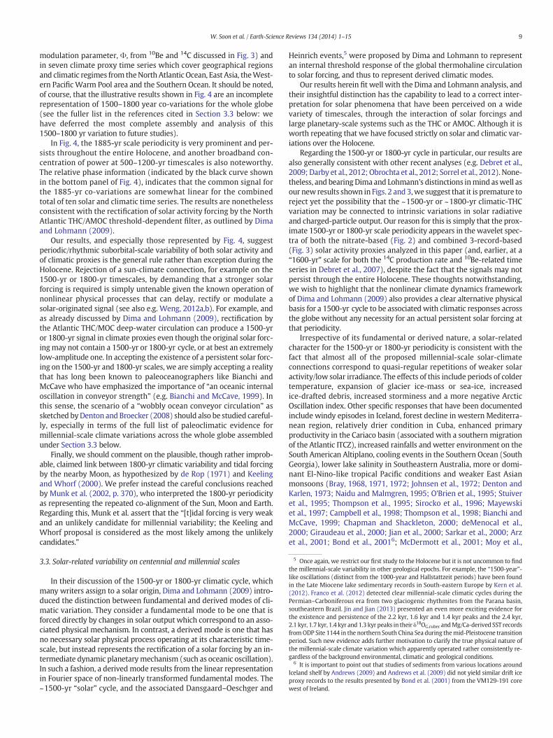
Table 1 lists a summary of the three solar activity and seven climateproxies that we study in this paper. Fig. 1 shows the time series of allthese 10 time series in their original units and can serve as further clar-ification of the highly clumped, solar and climatic time series plotted atthe top panels of Figs. 3 and 4, respectively.

2.1. Three Solar Activity Proxies: Nitrate Talos Dome Ice Core (TALDICE),solar modulation parameter from 10Be and 14C

We consider first the nitrate concentration record from TALDICE icecore (Talos Dome, East Antarctica, 72° 49′ S, 159° 11′ E, 2315 m a.s.l.),which covers roughly the last two glacial–interglacial cycles. The TalosDome site is found to be suitable for retrieving a reliable data seriesfor nitrate, at least in the Holocene period because its glaciological char-acteristics allow the preservation of this species in the snow layers(Stenni et al., 2002; Traversi et al., 2012). The nitrate content in such afavorable location is proposed to be mostly affected by changes of itsproduction in thepolar atmosphere by cosmic rays, and thus by solar ac-tivity, on multi-decadal to millennial time scales (Traversi et al., 2012).The link between nitrate in polar ice and solar activity is however stilla debated issue, because multiple sources and post-depositional pro-cesses that affect nitrate make it rare to have available a fully reliableand long enough record to investigate its variability across all timescales from decadal to multi-millennial. Moreover, a complete modeldescribing nitrate production and transport from the polar stratosphereis not available so far. Here, however, we stress that the relation be-tween nitrate and solar activity on the long-term scale is completely dif-ferent from that caused by solar energetic particle events on the time

to wavelet analysis in the present study.

End date(BP)

Resolution(years)

Proxy used Reference

11,400 12–30 Nitrate (NO−3) Traversi et al. (2012)

9812 1–10 Relative Gray Index (RGI) Selvaraj et al. (2007, 2011)

32,513 84–913 Total organic carbon (TOC) Kao et al. (2005)

9279 25 10Be Vonmoos et al. (2006)

11,405 10 14C Usoskin and Kromer (2005);Usoskin et al. (2007)

10,388 25–211 Sortable silt mean size(10–63 μm)

Bianchi and McCave (1999)

10,550 70 Percentages of lithic grainsor Ice-rafted debris

Bond et al. (2001)

14,875 250 Mg/Ca derived SST record Stott et al. (2004)

10,984 38 G. bulloides δ18O Moros et al. (2009)

10,984 38 G. ruber δ18O Moros et al. (2009)

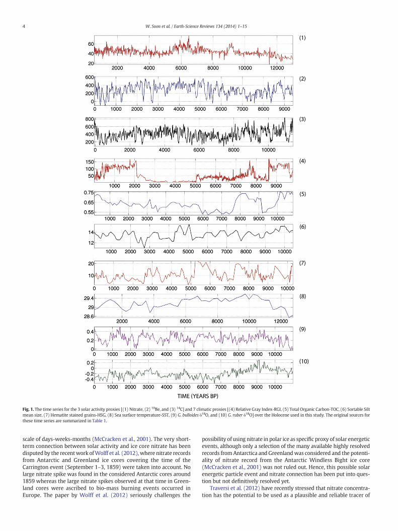
Fig. 1. The time series for the 3 solar activity proxies [(1) Nitrate, (2) 10Be, and (3) 14C] and 7 climatic proxies [(4) Relative Gray Index-RGI, (5) Total Organic Carbon-TOC, (6) Sortable Siltmean size, (7) Hematite stained grains-HSG, (8) Sea surface temperature-SST, (9) G. bulloides δ18O, and (10) G. ruber δ18O] over the Holocene used in this study. The original sources forthese time series are summarized in Table 1.

4 W. Soon et al. / Earth-Science Reviews 134 (2014) 1–15

scale of days-weeks-months (McCracken et al., 2001). The very short-term connection between solar activity and ice core nitrate has beendisputed by the recentwork ofWolff et al. (2012), where nitrate recordsfrom Antarctic and Greenland ice cores covering the time of theCarrington event (September 1–3, 1859) were taken into account. Nolarge nitrate spike was found in the considered Antarctic cores around1859 whereas the large nitrate spikes observed at that time in Green-land cores were ascribed to bio-mass burning events occurred inEurope. The paper by Wolff et al. (2012) seriously challenges the

possibility of using nitrate in polar ice as specific proxy of solar energeticevents, although only a selection of the many available highly resolvedrecords fromAntarctica and Greenlandwas considered and the potenti-ality of nitrate record from the Antarctic Windless Bight ice core(McCracken et al., 2001) was not ruled out. Hence, this possible solarenergetic particle event and nitrate connection has been put into ques-tion but not definitively resolved yet.

Traversi et al. (2012) have recently stressed that nitrate concentra-tion has the potential to be used as a plausible and reliable tracer of

5W. Soon et al. / Earth-Science Reviews 134 (2014) 1–15

solarmagnetic variations on awide range of timescales (see also Lalurajet al., 2011). Ogurtsov and Oinonen (2014) recently reported “distinctcentury-scale (50–150 yr) variability” in nitrate record of Laluraj et al.(2011) fromEast Antarctica and another record fromCentral Greenland.Based on this assumption of solar activity-nitrate link, Traversi et al.(2012) have shown that nitrate concentration yields higher correlationsand coherency with the two cosmogenic isotopes that represent stan-dard solar proxies (14C and 10Be) thanwith any regional climate proxies(see the results in Table 1 of that paper).We shall also adopt this generalassumption, and we provide below additional analysis and discussionon the connection of nitrate to both the solar modulation parameter,Φ (see the formalism in Usoskin et al., 2005), derived from 10Be of theGreenland Ice Core Project (Vonmoos et al., 2006), and to 14C produc-tion rates (Usoskin and Kromer, 2005; Usoskin et al., 2007), especiallyat the 1000, 1500–1800 and 2300 year timescales.

Using firn core data, Traversi et al. (2012) have already related solaractivity signals in the nitrate proxy to the modulation of the 11-yrSchwabe and 50–100-yr Gleissberg–Yoshimura cycles, but strong inter-annualmeteorological noisemakes the detection and resolution of suchcycles hard to confirm.4 This is why we have focused our study on icecore samples from 73 to 665 meter depth, roughly corresponding tothe Holocene interval from 560 to 11,400 years BP. The sampling reso-lution across this interval averages 20 years.

We have also assumed in this study that all three of the solar activityproxies adopted represent intrinsic changes in the Sun's magnetism. Atthe same time, we leave open the question posed by St-Onge et al.(2003) as to whether plausible coherence exists between the Earth'srelative paleomagnetic intensity index and the 10Be and 14C-relatedtime series on 1250-yr and 420-yr timescales. The recent picturesketched by Panovska et al. (2013), who suggested that Holocene geo-magnetic records possessed not discrete periods but a continuousbroadband spectrumwith a power law exponent of−2.3 ± 0.6 for pe-riods from 300 to 4000 years, certainly add a healthy dose of caution toany simplistic interpretation or premature conclusion.

2.2. Choice of Holocene paleoclimatic time series from regions of the EastAsian Monsoon, North Atlantic Ocean, Western Pacific Warm Pool andSouthern Ocean

2.2.1. Relative Gray Index (RGI) time series (Retreat Lake, Taiwan)The RGI is a measure of the degree of sediment lightening or darken-

ing, and usually reflects the relative proportion of organic to inorganic/minerogenic materials present in sediments. In the subalpine lake sedi-ments of Taiwan, this ratio primarily depends on the catchment vegeta-tion type (C3 and C4), as well as the intensity of erosion and weatheringof rocks in the catchment; both processes are intimately related to thestrength of the East Asian monsoon (EAM). For these reasons, we inter-pret the RGI data as a proxy for the varying intensity of the summer com-ponent of EAM conditions in subtropical Taiwan (Lou and Chen, 1997).

On our adopted RGI scale of 0 (dark) to 255 (white), higher RGIvalues (N80–170) between ~170 and 155 cm and in the top ~45 cm ofthe time series studied, indicate the presence of lighter (TOC content~ 2% with lower C3/C4 ratio) more minerogenic (Al content ~8–10%)sediment during the early and late Holocene intervals, respectively.These intervals correspond to cool-wet and cool-dry climates and a rel-atively weak EAM in subtropical Taiwan. By contrast, the low RGI values(b80) that characterize sediments between ~155 and 45 cm of the coreidentify the presence of organic-rich (TOC content ~40% with higherC3/C4 ratio), peaty sediments. The dark, peaty sediments cored inTaiwan indicate the presence of dense C3 vegetation in the catchment,which is nourished during strong monsoon seasons. In turn, the samemonsoonal signal is reflected by enhanced total organic carbon contentand a lowered carbon isotope (δ13C) value, as shown by earlier

4 It is also clear that the detection of any periodicities depend on the quality of datasetsand the methods of analysis adopted.

measurements on sediments from the same lake (Selvaraj et al., 2007,2011). Our interpretation of such paleoclimatic proxies is broadly simi-lar to vegetation changes during the Holocene that have been describedfrom South Korea (see e.g., Lim et al., 2012, 2013).

The RGI record from Retreat Lake provides a complete Holocene re-cord at better than decadal resolution. The record documents the pres-ence of a mid-Holocene period of optimum climate (~7500–5500 cal yrBP), when enhanced monsoonal activity occurred, and a number ofweak monsoon intervals before ca. 9400 and at 8200, 6900, 5500–4500and 3500 cal yr BP, some of which also occur in other high resolutionAsian monsoon records (e.g. Gupta et al., 2003; Wang et al., 2005).

2.2.2. Total Organic Carbon (TOC) time series (Okinawa Trough)A Holocene TOC time series has been reconstructed from a piston

core (MD012403) raised by RV Marion Dufresne during May, 2001from a water depth of 1420 m in the southern part of the OkinawaTrough (122.28° E, 25°07 N) (Kao et al., 2005). The core chronologyback to the Last Glacial Maximum (LGM) has been firmly establishedbased upon accelerator mass spectrometry radiocarbon (AMS 14C) dat-ing of planktonic foraminifers (Globigerinoides and Orbulina universa).

Based on the sedimentary TOC, TOC/total nitrogen (TN) ratio andtotal sulfur (TS) time series, Kao et al. (2005) observed low TS contentin sediments of the Holocene compared to sediments of the last glacialperiod. Further they showed that low TS content during the Holocenewas not controlled by TOC (refer Fig. 2 in Kao et al., 2005), since theTOC content of marine sediments primarily represents residual organicmaterial that has been oxidized to varying degrees along a variety ofpathways (i.e. oxygen, iron and sulfate). Although the Okinawa TOCcontent varied insignificantly after the LGM, distinctly low TS contentin the Holocene part of the core indicates that less organic materialwas mineralized via sulfate reduction then, which in turn can be in-ferred to result from an intensification of the Kuroshio Current (KC), to-gether with a parallel enhancement of deepwater circulation.

By providing additional oxygen to maintain a higher redox potentialat the sediment water interface, such oceanographic conditions dimin-ished sulfate reduction during the Holocene, a time when the EastAsian monsoon was also intensified as a result of increased NorthernHemisphere insolation (Berger and Loutre, 1991). Therefore, the in-creased EAM inferred from the RGI record from Taiwan and the intensi-fied KC phases implicated from TOC and TS records from the southernOkinawa Trough act in the same direction as the KC. Together, theseprocesses carry huge amounts of heat from the equatorial Pacific tothe northern North Pacific; thereby, strongly influencing climate overa wide region of East Asia and the northwest Pacific Ocean.

Noting these climatic links, we selected the RGI and TOC time seriesfor wavelet analysis in order to identify any periodicities that may per-tain to climate-forcing mechanisms, and especially to solar forcing ofthe East Asian monsoonal hydroclimate during the Holocene.

2.2.3. Other time seriesIn addition to the RGI record from Retreat Lake and TOC record from

Okinawa Trough,we have also included in our analysis several other keyclimatic and oceanic proxies. These are derived from the North AtlanticOcean – the sortable silt index (SSI) time series of Bianchi and McCave(1999) and the 4-records stacked drift ice index of Bond et al. (2001),the western Pacific Warm Pool – the 3-core records stacked sea surfacetemperature (SST) series of Stott et al. (2004), and the SouthernOcean –

time series of δ18O in Globigerina bulloides and Globigerinoides ruberfrom a deep sea sediment core collected from Murray Canyon offSouth Australia by Moros et al. (2009).

2.2.4. Multiple-Cross-wavelet for time-frequency analysis with multipletime series

We introduce here a new algorithm that is designed to analyzemultiple time series in time-frequency space. This algorithm is clearlya more efficient and effective method of examining common and

6 W. Soon et al. / Earth-Science Reviews 134 (2014) 1–15

coherent signals inmultiple time series thanwas able to be provided byprevious, simpler algorithms that only allow computation based on in-formation from amplitude of each time series. Some brief introductionand discussion of using wavelet transform for time series analysis canbe found in Frick et al. (1997) and Soon et al. (1999).

Here we use the Morlet wavelet as the mother function (ψ0(η))because it provides a higher periodicity (frequency) resolution and be-cause it is complex, which allows us to calculate the phase information(Soon et al., 2011). The Morlet wavelet ψ0(η), which consists of a com-plex exponential function modulated by a Gaussian, is defined as:

ψ0 ηð Þ ¼ π−14 eiω0 ηe

−η2

2

where η is a nondimensional “time” (Torrence and Compo, 1998). Forthe Morlet wavelet to be a mother wavelet, it must have finite energyand a zero mean (i.e., satisfying the admissibility condition, ω0 = 6(Farge, 1992).

The cross wavelet analysis, as introduced by Hudgins et al. (1993)and defined for two time series X1 and X2, with wavelet transforms(WX1 ) and (WX2 ), respectively, is:

WX1X2 ¼ WX1W�

X2;

where (*) denotes complex conjugation. Torrence and Webster(1999) defined the cross-wavelet energy as, WX1X2

n

��� ���2.For analysis of two (X1 and X2) ormore time series (X1, X2, X3,…, Xm),

the multi cross-wavelet was used which measures the common poweramong these time series accounting for the synchronization in phase,frequency and/or amplitude.

We define the multiple cross wavelets as:

WX1 ;X2 ;X3 ;…;Xm ¼ WFi∏n

k¼1W�

Gk

� �;

where F(t) andG(t) are matrices within which each element representsa time-dependent function itself and b ∙ N indicates an average of themultiple cross wavelets.

The phase angle ofWX1 ;X2 ;X3 ;…;Xm describes the phase relationship be-tween the X1, X2, X3,…, and Xm series in time–frequency space. The sta-tistical significance of the multiple-cross wavelet is estimated usingMonte Carlo methods with red noise to determine the 5% significancelevel (Torrence and Webster, 1999).

The arrows in the multiple-cross-wavelet spectra show on averagethe degree of linear or nonlinear dependence between the X1, X2, X3,…,and Xm in time–frequency space and the phase among these time series:arrows at 0° (pointing to the right) indicate that both time series are per-fectly positively correlated (in phase) and arrows at 180° (pointing to theleft) indicate that they are perfectly negatively correlated (180° out ofphase). It is important to understand that these two perfect casesimply a linear relationship between the considered phenomena. Non-horizontal arrows indicate an out of phase situation, meaning that thestudied phenomena have a more complex non-linear relationship.

The mathematical basis of the new multiple-cross-wavelet algo-rithm is a generalization of Wiener (1930)'s original cross function,but we compute in time–frequency space. Also, instead of consideringthe functions F and G, we consider two matrices F(t) and G(t). We de-scribe in the Appendix A the details of our new algorithm, togetherwith calculations and some tests that have been applied to it.

3. Results and discussion

3.1. Wavelet spectra of three solar proxies

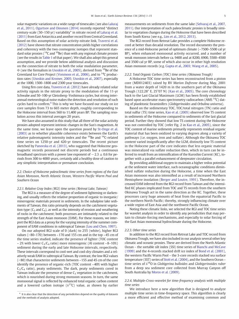
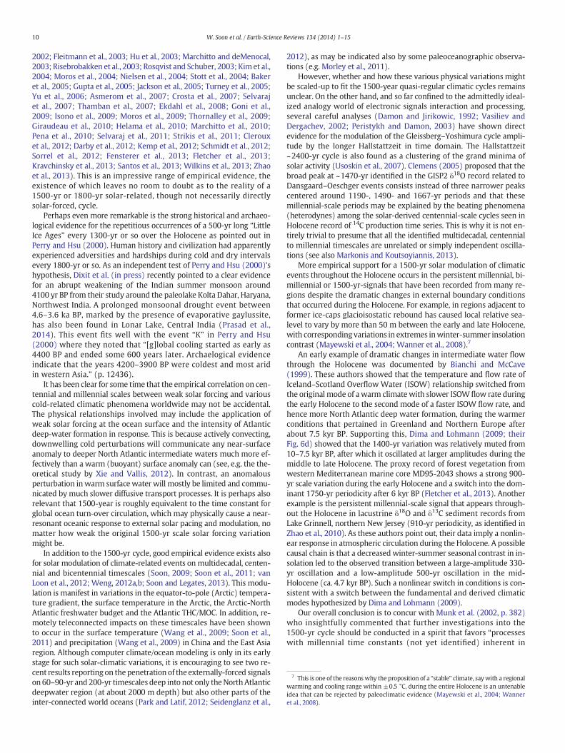
Fig. 2 shows the wavelet spectrum for the new solar activity proxybased on nitrate concentration. Concentrations of power occur at3358-yr and 1585-yr, across a broad-band peak that ranges from

about 900-yr to 500-yr, 120–140-yr, and at roughly the Gleissberg–Yoshimura 50–100 yr periodicity. All of these frequencies are potential-ly physically relevant for linking climate to intrinsic variations ofthe Sun's magnetic activity. We note that both the 1585-yr and50–100-yr cycles present in the solar nitrate proxy agreewith previous-ly recognized solar periodicities, namely the 1500-yr and 93-yr periodsfound for a surface salinity proxy from Florida Straits for the early-to-mid Holocene interval of 9.1 to 6.2 kyr BP (Schmidt et al., 2012; theseauthors also identified 87-yr and 60-yr peaks in their high-resolutiondata series). Using the solar modulation potential function for the past9400 years, determined from the two cosmogenic radionuclides 10Beand 14C, Abreu et al. (2012) found the periodicities of 88, 104, 150and 506 years using the Fourier Transform method and Hanslmeieret al. (2013) using wavelet analysis reported the period of about1000 years, Velasco Herrera (2013) also applying wavelet transformfound periodicities of 60, 128, 240, 480, 1000 and 2100 years.

Themost surprising andnovel aspect of our results in Fig. 2 is the de-tection of 1500-yr cycles in a new solar activity proxy record. Wemakethis identification cautiously because it is not yet fully established thatthis periodicity is physically connected to solar magnetism, despite theencouraging presence of 1500-yr cycles in a recent toy-model of a non-linear solar dynamo (Pipin et al., 2012). Brandenburg and Spiegel(2008), using another toy αω-dynamo model, have provided evidencefor the possible existence of 200–500 year solar magnetic variation, afrequency that is observedwhen their model is parameterized to adjustfor the long-term memory of the so-called α-effect. It remains a chal-lenge for solar physics to fully explore, and demonstrate the robustnessof, the possible 200–500 year and likely 1500-yr quasi-regular oscilla-tions in the Sun's magnetic and radiative outputs. In the meantime,however, little doubt now exists that fluctuations at these intervalsare present in proxy-climate datasets.

In general, the solar dynamo theory supports the idea that long-termquasi-periodic variations of solar magnetic activity can result from thenonlinear interplay between the magnetic field, differential rotationand helical convective motions. The most important timescales are re-lated to the time taken to re-establish the angular momentum balance(differential rotation) and the magnetic helicity balance (associatingwith the α-effect) in the convection zone caused by perturbations inthe large-scale magnetic field. Both processes, i.e. relaxation of the an-gular momentum transport and the magnetic helicity balance, corre-spond to about 10 solar cycles (see, Pipin, 1999; Pipin et al., 2012).Pipin et al. (2012) also found that a combination of the random fluctu-ations of the dynamo governing parameters and the nonlinear relaxa-tion of the principal dynamo mechanisms can produce the quasi-periodic variations on millennial timescales. However, the stability ofthe revealed periods can be questioned, because the dynamo may be-come non-stationary under random fluctuations. Moreover, it happensthat the dynamical properties of the solar dynamo on the millennialtimescale look very similar to the properties of the Brownian motions(Pipin et al., 2013). This is another reason why we think our currentchoice of subjective wordings in describing solar and climate variationsas noted under footnote 3 is more physically accurate and honest thanany deliberate attempt to impose a falsely precise vocabulary.

Given the relatively short time series considered in Fig. 2 (or seeFig. 1 for all the ten series), the prominent 3358-yr peak in the nitratesolar activity proxy (Fig. 2) may be given less scientific weight. How-ever, results from previous researchers suggest that it may also repre-sent a real feature. For example, Stuiver et al. (1995) have recorded a3300-yr period in their Holocene bidecadal-resolution record of δ18Ofrom GISP2, and Mayewski et al. (1997) reported a highly significantpeak at 3200-yr in a record of Holocene polar circulation. Clerouxet al. (2012) show the presence of the 3300-year period for aδ18Oseawater Holocene series from the sediment core off Cape Hatteras(although the 3300-yr scale obviously lies outside the cone-of-influence of their wavelet analysis where edge effects, owing to a finitelength of time series, become important). Finally, a roughly 3000-yr

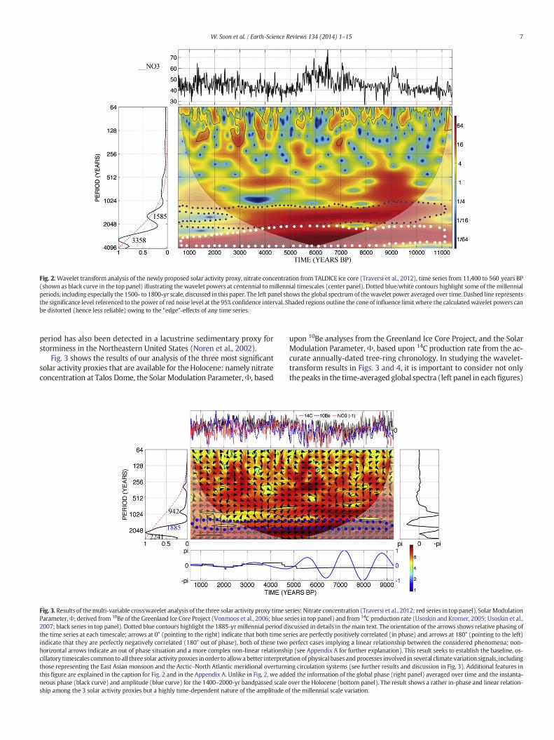
Fig. 2.Wavelet transform analysis of the newly proposed solar activity proxy, nitrate concentration from TALDICE ice core (Traversi et al., 2012), time series from 11,400 to 560 years BP(shown as black curve in the top panel) illustrating the wavelet powers at centennial tomillennial timescales (center panel). Dotted blue/white contours highlight some of the millennialperiods, including especially the 1500- to 1800-yr scale, discussed in this paper. The left panel shows the global spectrum of thewavelet power averaged over time. Dashed line representsthe significance level referenced to the power of red noise level at the 95% confidence interval. Shaded regions outline the cone of influence limitwhere the calculatedwavelet powers canbe distorted (hence less reliable) owing to the “edge”-effects of any time series.

7W. Soon et al. / Earth-Science Reviews 134 (2014) 1–15

period has also been detected in a lacustrine sedimentary proxy forstorminess in the Northeastern United States (Noren et al., 2002).

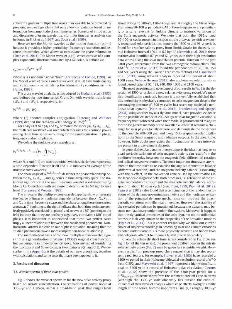
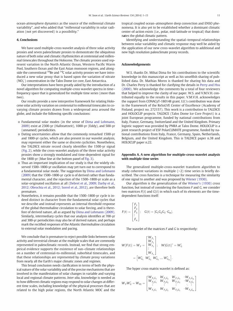
Fig. 3 shows the results of our analysis of the three most significantsolar activity proxies that are available for the Holocene: namely nitrateconcentration at Talos Dome, the Solar Modulation Parameter,Φ, based

Fig. 3. Results of themulti-variable crosswavelet analysis of the three solar activity proxy time sParameter,Φ, derived from 10Be of the Greenland Ice Core Project (Vonmoos et al., 2006; blue s2007; black series in top panel). Dotted blue contours highlight the 1885-yrmillennial period dthe time series at each timescale; arrows at 0° (pointing to the right) indicate that both time seindicate that they are perfectly negatively correlated (180° out of phase), both of these twohorizontal arrows indicate an out of phase situation and a more complex non-linear relationshcillatory timescales common to all three solar activity proxies in order to allowa better interpretthose representing the East Asian monsoon and the Arctic–North Atlantic meridional overturnthis figure are explained in the caption for Fig. 2 and in the Appendix A. Unlike in Fig. 2, we addneous phase (black curve) and amplitude (blue curve) for the 1400–2000-yr bandpassed scaleship among the 3 solar activity proxies but a highly time-dependent nature of the amplitude o

upon 10Be analyses from the Greenland Ice Core Project, and the SolarModulation Parameter, Φ, based upon 14C production rate from the ac-curate annually-dated tree-ring chronology. In studying the wavelet-transform results in Figs. 3 and 4, it is important to consider not onlythepeaks in the time-averaged global spectra (left panel in each figures)

eries: Nitrate concentration (Traversi et al., 2012; red series in top panel), SolarModulationeries in top panel) and from 14C production rate (Usoskin and Kromer, 2005; Usoskin et al.,iscussed in details in themain text. The orientation of the arrows shows relative phasing ofries are perfectly positively correlated (in phase) and arrows at 180° (pointing to the left)perfect cases implying a linear relationship between the considered phenomena; non-ip (see Appendix A for further explanation). This result seeks to establish the baseline, os-ation of physical bases and processes involved in several climate variation signals, includinging circulation systems (see further results and discussion in Fig. 3). Additional features ined the information of the global phase (right panel) averaged over time and the instanta-over the Holocene (bottom panel). The result shows a rather in-phase and linear relation-f the millennial scale variation.

Fig. 4. Results of the multi-variable cross wavelet analysis of the nitrate, 10Be and 14C solar activity proxies and a total of seven paleoclimatic series from the North Atlantic (sortable siltmean size series from Bianchi and McCave, 1999; and stacked drift ice indices in Bond et al., 2001), Western Pacific Warm Pool (stacked SST series from Stott et al., 2004), East AsianMonsoon (Relative Gray Index series from Retreat Lake in Taiwan and Total organic carbon content in sea sediment from Okinawa Trough; see Kao et al., 2005) and Southern Ocean(δ18O in Globigerina bulloides and Globigerinoides ruber, from deep sea sediment core at Murray Canyon off southern Australia; see Moros et al., 2009). Dotted blue contours highlightthe 1500–1800-yr time scales discussed in this paper. For explanation of arrow orientations, see caption to Fig. 3, and the Appendix A. Additional features in this figure are explainedin the captions for Figs. 2 and 3.

8 W. Soon et al. / Earth-Science Reviews 134 (2014) 1–15

but also the instantaneous time-frequency spectra shown in the centralpanel of Figs. 3 and 4.

Several prominent common signals occur in Fig. 3. First, the signal ofthe 1885-yr periodicity has strong time dependence in the amplitude ofits variation, with relatively larger amplitude during the early to mid-Holocene and relatively muted amplitude for late Holocene (see bluecurve in the bottom panel of Fig. 3). This signal can only be obtainedusing the unique, inverse multiple cross wavelet transforms presentedhere. It is important to highlight the fact that a common 1800-yr solarvariation timescale has been captured by three very different solar prox-ies which represent different geographic and climatic parts of theEarth's climate system. The most important result concerning the1800-yr scale variation from Fig. 3 is its relatively in-phase or linear re-lationship (see black curve in the bottom panel of Fig. 3) for the threedifferent solar activity proxies. This result, in turn, emphasizes the pace-maker role of the solar activity forcing on millennial scale rather thanany strict persistence from the sense of amplitude modulation throughthe solar radiative forcing on Earth climatic responses.

Our independent result therefore reaffirms the conclusion and anal-yses in Traversi et al. (2012), and our conclusion on the clear time-dependence of the amplitude of the 1885-yr millennial scale variationis also broadly consistent with the previous results of Debret et al.(2007, 2009).

If only one of the solar proxies showed a coherence at ~1800-yr withclimatic indices, this might reflect a regional climatic influence upon theproxy record. However, since all the three proxy series showa similar re-lation, and since each has quite a different fate in the terrestrial system(nitrate are expected to be mostly affected by the tropospheric airmass transport and snow deposition in Antarctica; 10Be—by stratospher-ic air mass transport and snow deposition in Greenland; 14C—mostly bythe global ocean circulation), a tripartite simultaneous influence of re-gional climate on the proxy data sets is unlikely. Accordingly, we viewthe 1500–1800-yr scale as representing a fundamental periodicity ofthe spectrum of solar variation rather than a mere derived mode in theframework of Dima and Lohmann (2009; see further discussion inSection 3.2 and 3.3 below).

Fig. 3 also exhibits significant spectral power on timescales of2200–2400-yr, 1000-yr, 500–700-yr, 350-yr, 120-yr and 50–100-yr.Almost without exception, the amplitudes of all these periodicities

vary over time during the Holocene. This empirical observation impliesa very rich nonlinear interaction for the relevant underlying physicalprocesses and dynamics, without the predominance of any particularoperational timescales.

3.2. Wavelet spectra of individual paleoclimatic data-series

Before discussing the master multiple-cross-wavelet analysis basedupon the three solar proxy time series and seven paleoclimatic records(Section 3.3 and Fig. 4), we comment first on the wavelet spectra thatoccur in some of the individual climate proxies used in this study,since most of them have not been previously published and discussed.

First, wavelet analysis of δ18O in the Globigerina bulloides record iden-tifies a dominant 1585-yr scale power, which is closely similar to the1567-yr signal reported previously using conventional Fourier-basedtime series analysis (Moros et al., 2009). The wavelet analysis also iden-tifies a further significant concentration of power at about 560-yr inthis series. Applying wavelet analysis to the available δ18O record forthe planktonic species Globigerinoides ruber from the same sedimentcore identifies prominent concentrations of power at about 2048-yr,1000-yr and 512-yr, consistent with our other results and with solar ac-tivity forcing.

Second, direct wavelet analysis of the composite Western PacificWarm Pool SST time series (binned MD81, MD 76 andMD 70 Holoceneseries) of Stott et al. (2004) also identifies a convincing signal at the1800-yr scale that persists throughout the Holocene. A similar 1800-yrvariability is also found in the East Asian monsoonal RGI index fromRetreat Lake, and an 1800-yr periodicity also appears in the Holocenewavelet spectrum for the SST-Mg/Ca proxy from Cape Hatteras pub-lished in Cleroux et al. (2012). Finally, the direct wavelet analysis ofthe sortable silt size time series (a direct proxy for the North AtlanticTHC/AMOC) from the NEAP-15 K core in Bianchi and McCave (1999)yields not only a prominent 1400-yr periodicity, but also significantpeaks at 700-yr and 2700-yr scales.

Fig. 4 presents these results, and the co-variations of all the solar andclimatic proxy series, in compact form in a single chart. With the aid ofthe newmultiple-cross-wavelet algorithm, we have been able to study,in a consistentway and for the first time, the common signals containedin three different solar activity proxies (nitrate concentration and solar

5 Once again, we restrict our first study to the Holocene but it is not uncommon to findthe millennial-scale variability in other geological epochs. For example, the “1500-year”-like oscillations (distinct from the 1000-year and Hallstattzeit periods) have been foundin the Late Miocene lake sedimentary records in South-eastern Europe by Kern et al.(2012). Franco et al. (2012) detected clear millennial-scale climatic cycles during thePermian–Carboniferous era from two glaciogenic rhythmites from the Parana basin,southeastern Brazil. Jin and Jian (2013) presented an even more exciting evidence forthe existence and persistence of the 2.2 kyr, 1.6 kyr and 1.4 kyr peaks and the 2.4 kyr,2.1 kyr, 1.7 kyr, 1.4 kyr and 1.3 kyr peaks in their δ18OG.ruber andMg/Ca-derived SST recordsfromODP Site 1144 in the northern South China Sea during themid-Pleistocene transitionperiod. Such new evidence adds further motivation to clarify the true physical nature ofthe millennial-scale climate variation which apparently operated rather consistently re-gardless of the background environmental, climatic and geological conditions.

6 It is important to point out that studies of sediments from various locations aroundIceland shelf by Andrews (2009) and Andrews et al. (2009) did not yield similar drift iceproxy records to the results presented by Bond et al. (2001) from the VM129-191 corewest of Ireland.

9W. Soon et al. / Earth-Science Reviews 134 (2014) 1–15

modulation parameter, Φ, from 10Be and 14C discussed in Fig. 3) andin seven climate proxy time series which cover geographical regionsand climatic regimes from theNorth Atlantic Ocean, East Asia, theWest-ern Pacific Warm Pool area and the Southern Ocean. It should be noted,of course, that the illustrative results shown in Fig. 4 are an incompleterepresentation of 1500–1800 year co-variations for the whole globe(see the fuller list in the references cited in Section 3.3 below: wehave deferred the most complete assembly and analysis of this1500–1800 yr variation to future studies).

In Fig. 4, the 1885-yr scale periodicity is very prominent and per-sists throughout the entire Holocene, and another broadband con-centration of power at 500–1200-yr timescales is also noteworthy.The relative phase information (indicated by the black curve shownin the bottom panel of Fig. 4), indicates that the common signal forthe 1885-yr co-variations are somewhat linear for the combinedtotal of ten solar and climatic time series. The results are nonethelessconsistent with the rectification of solar activity forcing by the NorthAtlantic THC/AMOC threshold-dependent filter, as outlined by Dimaand Lohmann (2009).

Our results, and especially those represented by Fig. 4, suggestperiodic/rhythmic suborbital-scale variability of both solar activity andof climatic proxies is the general rule rather than exception during theHolocene. Rejection of a sun-climate connection, for example on the1500-yr or 1800-yr timescales, by demanding that a stronger solarforcing is required is simply untenable given the known operation ofnonlinear physical processes that can delay, rectify or modulate asolar-originated signal (see also e.g. Weng, 2012a,b). For example, andas already discussed by Dima and Lohmann (2009), rectification bythe Atlantic THC/MOC deep-water circulation can produce a 1500-yror 1800-yr signal in climate proxies even though the original solar forc-ingmay not contain a 1500-yr or 1800-yr cycle, or at best an extremelylow-amplitude one. In accepting the existence of a persistent solar forc-ing on the 1500-yr and 1800-yr scales, we are simply accepting a realitythat has long been known to paleoceanographers like Bianchi andMcCave who have emphasized the importance of “an oceanic internaloscillation in conveyor strength” (e.g. Bianchi and McCave, 1999). Inthis sense, the scenario of a “wobbly ocean conveyor circulation” assketched byDenton and Broecker (2008) should also be studied careful-ly, especially in terms of the full list of paleoclimatic evidence formillennial-scale climate variations across the whole globe assembledunder Section 3.3 below.

Finally, we should comment on the plausible, though rather improb-able, claimed link between 1800-yr climatic variability and tidal forcingby the nearby Moon, as hypothesized by de Rop (1971) and Keelingand Whorf (2000). We prefer instead the careful conclusions reachedby Munk et al. (2002, p. 370), who interpreted the 1800-yr periodicityas representing the repeated co-alignment of the Sun, Moon and Earth.Regarding this, Munk et al. assert that the “[t]idal forcing is very weakand an unlikely candidate for millennial variability; the Keeling andWhorf proposal is considered as the most likely among the unlikelycandidates.”

3.3. Solar-related variability on centennial and millennial scales

In their discussion of the 1500-yr or 1800-yr climatic cycle, whichmany writers assign to a solar origin, Dima and Lohmann (2009) intro-duced the distinction between fundamental and derived modes of cli-matic variation. They consider a fundamental mode to be one that isforced directly by changes in solar output which correspond to an asso-ciated physical mechanism. In contrast, a derived mode is one that hasno necessary solar physical process operating at its characteristic time-scale, but instead represents the rectification of a solar forcing by an in-termediate dynamic planetarymechanism (such as oceanic oscillation).In such a fashion, a derivedmode results from the linear representationin Fourier space of non-linearly transformed fundamental modes. The~1500-yr “solar” cycle, and the associated Dansgaard–Oeschger and

Heinrich events,5 were proposed by Dima and Lohmann to representan internal threshold response of the global thermohaline circulationto solar forcing, and thus to represent derived climatic modes.

Our results herein fit well with the Dima and Lohmann analysis, andtheir insightful distinction has the capability to lead to a correct inter-pretation for solar phenomena that have been perceived on a widevariety of timescales, through the interaction of solar forcings andlarge planetary-scale systems such as the THC or AMOC. Although it isworth repeating that we have focused strictly on solar and climatic var-iations over the Holocene.

Regarding the 1500-yr or 1800-yr cycle in particular, our results arealso generally consistent with other recent analyses (e.g. Debret et al.,2009; Darby et al., 2012; Obrochta et al., 2012; Sorrel et al., 2012). None-theless, and bearing Dima and Lohmann's distinctions inmind aswell asour new results shown in Figs. 2 and 3,we suggest that it is premature toreject yet the possibility that the ~1500-yr or ~1800-yr climatic-THCvariation may be connected to intrinsic variations in solar radiativeand charged-particle output. Our reason for this is simply that the prox-imate 1500-yr or 1800-yr scale periodicity appears in the wavelet spec-tra of both the nitrate-based (Fig. 2) and combined 3-record-based(Fig. 3) solar activity proxies analyzed in this paper (and, earlier, at a“1600-yr” scale for both the 14C production rate and 10Be-related timeseries in Debret et al., 2007), despite the fact that the signals may notpersist through the entire Holocene. These thoughts notwithstanding,we wish to highlight that the nonlinear climate dynamics frameworkof Dima and Lohmann (2009) also provides a clear alternative physicalbasis for a 1500-yr cycle to be associated with climatic responses acrossthe globe without any necessity for an actual persistent solar forcing atthat periodicity.

Irrespective of its fundamental or derived nature, a solar-relatedcharacter for the 1500-yr or 1800-yr periodicity is consistent with thefact that almost all of the proposed millennial-scale solar-climateconnections correspond to quasi-regular repetitions of weaker solaractivity/low solar irradiance. The effects of this include periods of coldertemperature, expansion of glacier ice-mass or sea-ice, increasedice-drafted debris, increased storminess and a more negative ArcticOscillation index. Other specific responses that have been documentedinclude windy episodes in Iceland, forest decline in western Mediterra-nean region, relatively drier condition in Cuba, enhanced primaryproductivity in the Cariaco basin (associated with a southern migrationof the Atlantic ITCZ), increased rainfalls and wetter environment on theSouth American Altiplano, cooling events in the Southern Ocean (SouthGeorgia), lower lake salinity in Southeastern Australia, more or domi-nant El-Nino-like tropical Pacific conditions and weaker East Asianmonsoons (Bray, 1968, 1971, 1972; Johnsen et al., 1972; Denton andKarlen, 1973; Naidu and Malmgren, 1995; O'Brien et al., 1995; Stuiveret al., 1995; Thompson et al., 1995; Sirocko et al., 1996; Mayewskiet al., 1997; Campbell et al., 1998; Thompson et al., 1998; Bianchi andMcCave, 1999; Chapman and Shackleton, 2000; deMenocal et al.,2000; Giraudeau et al., 2000; Jian et al., 2000; Sarkar et al., 2000; Arzet al., 2001; Bond et al., 20016; McDermott et al., 2001; Moy et al.,

7 This is one of the reasonswhy the proposition of a “stable” climate, saywith a regionalwarming and cooling range within ±0.5 °C, during the entire Holocene is an untenableidea that can be rejected by paleoclimatic evidence (Mayewski et al., 2004; Wanneret al., 2008).

10 W. Soon et al. / Earth-Science Reviews 134 (2014) 1–15

2002; Fleitmann et al., 2003; Hu et al., 2003; Marchitto and deMenocal,2003; Risebrobakken et al., 2003; Rosqvist and Schuber, 2003; Kim et al.,2004; Moros et al., 2004; Nielsen et al., 2004; Stott et al., 2004; Bakeret al., 2005; Gupta et al., 2005; Jackson et al., 2005; Turney et al., 2005;Yu et al., 2006; Asmerom et al., 2007; Crosta et al., 2007; Selvarajet al., 2007; Thamban et al., 2007; Ekdahl et al., 2008; Goni et al.,2009; Isono et al., 2009; Moros et al., 2009; Thornalley et al., 2009;Giraudeau et al., 2010; Helama et al., 2010; Marchitto et al., 2010;Pena et al., 2010; Selvaraj et al., 2011; Strikis et al., 2011; Clerouxet al., 2012; Darby et al., 2012; Kemp et al., 2012; Schmidt et al., 2012;Sorrel et al., 2012; Fensterer et al., 2013; Fletcher et al., 2013;Kravchinsky et al., 2013; Santos et al., 2013; Wilkins et al., 2013; Zhaoet al., 2013). This is an impressive range of empirical evidence, theexistence of which leaves no room to doubt as to the reality of a1500-yr or 1800-yr solar-related, though not necessarily directlysolar-forced, cycle.

Perhaps even more remarkable is the strong historical and archaeo-logical evidence for the repetitious occurrences of a 500-yr long “LittleIce Ages” every 1300-yr or so over the Holocene as pointed out inPerry and Hsu (2000). Human history and civilization had apparentlyexperienced adversities and hardships during cold and dry intervalsevery 1800-yr or so. As an independent test of Perry and Hsu (2000)'shypothesis, Dixit et al. (in press) recently pointed to a clear evidencefor an abrupt weakening of the Indian summer monsoon around4100 yr BP from their study around the paleolake Kolta Dahar, Haryana,Northwest India. A prolonged monsoonal drought event between4.6–3.6 ka BP, marked by the presence of evaporative gaylussite,has also been found in Lonar Lake, Central India (Prasad et al.,2014). This event fits well with the event “K” in Perry and Hsu(2000) where they noted that “[g]lobal cooling started as early as4400 BP and ended some 600 years later. Archaelogical evidenceindicate that the years 4200–3900 BP were coldest and most aridin western Asia.” (p. 12436).

It has been clear for some time that the empirical correlation on cen-tennial and millennial scales between weak solar forcing and variouscold-related climatic phenomena worldwide may not be accidental.The physical relationships involved may include the application ofweak solar forcing at the ocean surface and the intensity of Atlanticdeep-water formation in response. This is because actively convecting,downwelling cold perturbations will communicate any near-surfaceanomaly to deeper North Atlantic intermediate waters much more ef-fectively than a warm (buoyant) surface anomaly can (see, e.g. the the-oretical study by Xie and Vallis, 2012). In contrast, an anomalousperturbation in warm surface water will mostly be limited and commu-nicated by much slower diffusive transport processes. It is perhaps alsorelevant that 1500-year is roughly equivalent to the time constant forglobal ocean turn-over circulation, which may physically cause a near-resonant oceanic response to external solar pacing and modulation, nomatter how weak the original 1500-yr scale solar forcing variationmight be.

In addition to the 1500-yr cycle, good empirical evidence exists alsofor solar modulation of climate-related events on multidecadal, centen-nial and bicentennial timescales (Soon, 2009; Soon et al., 2011; vanLoon et al., 2012; Weng, 2012a,b; Soon and Legates, 2013). This modu-lation is manifest in variations in the equator-to-pole (Arctic) tempera-ture gradient, the surface temperature in the Arctic, the Arctic-NorthAtlantic freshwater budget and the Atlantic THC/MOC. In addition, re-motely teleconnected impacts on these timescales have been shownto occur in the surface temperature (Wang et al., 2009; Soon et al.,2011) and precipitation (Wang et al., 2009) in China and the East Asiaregion. Although computer climate/ocean modeling is only in its earlystage for such solar-climatic variations, it is encouraging to see two re-cent results reporting on thepenetration of the externally-forced signalson 60–90-yr and 200-yr timescales deep into not only theNorthAtlanticdeepwater region (at about 2000 m depth) but also other parts of theinter-connected world oceans (Park and Latif, 2012; Seidenglanz et al.,

2012), as may be indicated also by some paleoceanographic observa-tions (e.g. Morley et al., 2011).

However, whether and how these various physical variations mightbe scaled-up to fit the 1500-year quasi-regular climatic cycles remainsunclear. On the other hand, and so far confined to the admittedly ideal-ized analogy world of electronic signals interaction and processing,several careful analyses (Damon and Jirikowic, 1992; Vasiliev andDergachev, 2002; Peristykh and Damon, 2003) have shown directevidence for the modulation of the Gleissberg–Yoshimura cycle ampli-tude by the longer Hallstattzeit in time domain. The Hallstattzeit~2400-yr cycle is also found as a clustering of the grand minima ofsolar activity (Usoskin et al., 2007). Clemens (2005) proposed that thebroad peak at ~1470-yr identified in the GISP2 δ18O record related toDansgaard–Oeschger events consists instead of three narrower peakscentered around 1190-, 1490- and 1667-yr periods and that thesemillennial-scale periods may be explained by the beating phenomena(heterodynes) among the solar-derived centennial-scale cycles seen inHolocene record of 14C production time series. This is why it is not en-tirely trivial to presume that all the identified multidecadal, centennialto millennial timescales are unrelated or simply independent oscilla-tions (see also Markonis and Koutsoyiannis, 2013).

More empirical support for a 1500-yr solar modulation of climaticevents throughout the Holocene occurs in the persistent millennial, bi-millennial or 1500-yr-signals that have been recorded from many re-gions despite the dramatic changes in external boundary conditionsthat occurred during the Holocene. For example, in regions adjacent toformer ice-caps glacioisostatic rebound has caused local relative sea-level to vary by more than 50 m between the early and late Holocene,with corresponding variations in extremes inwinter-summer insolationcontrast (Mayewski et al., 2004; Wanner et al., 2008).7

An early example of dramatic changes in intermediate water flowthrough the Holocene was documented by Bianchi and McCave(1999). These authors showed that the temperature and flow rate ofIceland–Scotland Overflow Water (ISOW) relationship switched fromthe original mode of a warm climatewith slower ISOW flow rate duringthe early Holocene to the second mode of a faster ISOW flow rate, andhence more North Atlantic deep water formation, during the warmerconditions that pertained in Greenland and Northern Europe afterabout 7.5 kyr BP. Supporting this, Dima and Lohmann (2009; theirFig. 6d) showed that the 1400-yr variation was relatively muted from10–7.5 kyr BP, after which it oscillated at larger amplitudes during themiddle to late Holocene. The proxy record of forest vegetation fromwestern Mediterranean marine core MD95-2043 shows a strong 900-yr scale variation during the early Holocene and a switch into the dom-inant 1750-yr periodicity after 6 kyr BP (Fletcher et al., 2013). Anotherexample is the persistent millennial-scale signal that appears through-out the Holocene in lacustrine δ18O and δ13C sediment records fromLake Grinnell, northern New Jersey (910-yr periodicity, as identified inZhao et al., 2010). As these authors point out, their data imply a nonlin-ear response in atmospheric circulation during the Holocene. A possiblecausal chain is that a decreased winter-summer seasonal contrast in in-solation led to the observed transition between a large-amplitude 330-yr oscillation and a low-amplitude 500-yr oscillation in the mid-Holocene (ca. 4.7 kyr BP). Such a nonlinear switch in conditions is con-sistent with a switch between the fundamental and derived climaticmodes hypothesized by Dima and Lohmann (2009).

Our overall conclusion is to concur with Munk et al. (2002, p. 382)who insightfully commented that further investigations into the1500-yr cycle should be conducted in a spirit that favors “processeswith millennial time constants (not yet identified) inherent in

11W. Soon et al. / Earth-Science Reviews 134 (2014) 1–15

ocean-atmosphere dynamics as the source of the millennial climatevariability”, and who added that “millennial variability in solar radi-ation (not yet discovered) is a possibility.”

4. Conclusions

We have used multiple-cross wavelet analysis of three solar activityproxies and seven paleoclimate proxies to demonstrate the ubiquitousnature of both solar and climatic rhythmicities at centennial andmillen-nial timescales throughout the Holocene. The climatic proxies used rep-resent variation in the North Atlantic Ocean, Western Pacific WarmPool, Southern Ocean and the East Asian monsoon regions, and along-side the conventional 10Be and 14C solar activity proxies we have intro-duced a new solar proxy that is based upon the variation of nitrate(NO3

−) concentration in the Talos Dome ice core, East Antarctica.Our interpretations have been greatly aided by the introduction of a

novel algorithm for computing multiple-cross wavelet spectra in time–frequency space that is generalized for multiple time series (more thantwo).

Our results provide a new interpretive framework for relating Holo-cene solar activity variation on centennial tomillennial timescales to co-varying climate proxies drawn from a widespread area around theglobe, and include the following specific conclusions:

o Fundamental solar modes (in the sense of Dima and Lohmann,2009) exist at 2300-yr (Hallstattzeit), 1000-yr (Eddy), and 500-yr(unnamed) periodicities.

o Dating uncertainties allow that the commonly remarked 1500-yrand 1800-yr cycles, which are also present in our wavelet analysis,may represent either the same or discrete cyclicities. Nonetheless,the TALDICE nitrate record clearly identifies the 1500-yr signal(Fig. 2), while the cross-wavelet analysis of the three solar activityproxies show a strongly modulated and time-dependent signal forthe 1800-yr (blue line at the bottom panel of Fig. 3).

o Thus an important implication of our study is that the widely ob-served 1500–1800-yr oscillation may yet turn out to correspond toa fundamental solar mode. The suggestion by Dima and Lohmann(2009) that the 1500–1800-yr cycle is of derived rather than funda-mental character, and the rejection of the 1500–1800-yr scale as asolar-originated oscillation at all (Debret et al., 2009; Darby et al.,2012; Obrochta et al., 2012; Sorrel et al., 2012), are therefore bothpremature.

o Nonetheless, it remains possible that the 1500–1800-yr cycle is in-deed distinct in character from the fundamental solar cycles thatwe describe and instead represents an internal threshold responseof the global thermohaline circulation to solar forcing, and is there-fore of derived nature, all as argued by Dima and Lohmann (2009).Similarly, intermediary cycles that our analysis identifies at 700-yrand 300-yr periodicities may also be of derived nature, and perhapsmark the rectified responses of the Atlantic thermohaline circulationto external solar modulation and pacing.

We conclude that is premature to reject possible links between solaractivity and terrestrial climate at the multiple scales that are commonlyrepresented in paleoclimatic records. Instead, we find that strong em-pirical evidence supports the existence of sun–climate relationshipson a number of centennial-to-millennial, suborbital timescales, andthat these relationships are represented by climate proxy variationsfrom nearly all the Earth's major climatic zones and regimes.

This broad conclusion needs clarification in terms of both the phys-ical nature of the solar variability and of theprecisemechanisms that areinvolved in the manifestation of solar changes in variable and varyinglocal and regional climate patterns. Inter alia, knowledge is needed asto howdifferent climatic regionsmay respond to solar changes at differ-ent time scales, including knowledge of the physical processes that arerelated to the high polar regions, the North Atlantic MOC and the

tropical coupled ocean–atmosphere deep convection and ENSO phe-nomena. It is also yet to be established whether a dominant climaticcenter-of-action exists (i.e., polar, mid-latitude or tropical) that domi-nates the global climatic pattern.

Identifying and understanding the spatial–temporal relationshipsbetween solar variability and climatic response may well be aided bythe application of our new cross-wavelet algorithm to additional andnew high resolution paleoclimate proxy records.

Acknowledgements

W.S. thanks Dr. Mihai Dima for his contributions to the scientificknowledge in this manuscript as well as his unselfish sharing of pub-lished data. Dr. Mathias Moros is thanked for sharing his data andDr. Charles Perry is thanked for clarifying the details in Perry and Hsu(2000). We acknowledge the comments by a total of four reviewersthat helped to improve the clarity of our paper. W.S. and V.M.V.H. con-tributed equally to the results in this paper. V.M.V.H. acknowledgesthe support from CONACyT-180148 grant. I.U.'s contribution was donein the framework of the ReSoLVE Center of Excellence (Academy ofFinland, project no. 272157). This work is a contribution to TALDICEand HOLOCLIP projects. TALDICE (Talos Dome Ice Core Project) is ajoint European programme, funded by national contributions fromItaly, France, Germany, Switzerland and the United Kingdom. Primarylogistic support was provided by PNRA at Talos Dome. HOLOCLIP is ajoint research project of ESF PolarCLIMATE programme, funded by na-tional contributions from Italy, France, Germany, Spain, Netherlands,Belgium, and the United Kingdom. This is TALDICE paper n.38 andHOLOCLIP paper n.22.

Appendix A. A new algorithm for multiple-cross-wavelet analysiswith multiple time series

The generalized multiple-cross-wavelet transform algorithm tostudy coherent variations in multiple (N2) time series is briefly de-scribed. The cross function is a technique for measuring the similarityof one signal to another and was proposed by Wiener (1930).

Our algorithm is the generalization of the Wiener's (1930) crossfunction, but instead of considering the functions F and G, we considertwo matrices F(t) and G(t) in which each of its elements are the time-dependent functions itself:

F tð Þ ¼

F1F2F3⋮Fn

266664

377775; G tð Þ ¼ G1G2G3⋯Gm½ �:

The wavelet of the matrices F and G is respectively:

W F tð Þ½ � ¼ WF ¼

WF1WF2WF3⋮WFn

266664

377775; W G tð Þ½ �� ¼ W�

G

¼ W�G1

W�G2

W�G3

…W�Gm

h i:

The hyper cross-matrix wavelet is defined as:

WFW�G ¼ WFG ¼

WF1G1WF1G2

WF1G3⋯WF1Gm

W F2G1WF2G2

WF1G3⋯WF1G1

⋮ ⋮ ⋮ ⋱ ⋮WFnG1

WFnG2WFnG3

⋯WFnGm

2664

3775

12 W. Soon et al. / Earth-Science Reviews 134 (2014) 1–15

where each element of the hyper cross-matrix are one cross waveletmatrix:

WFiGksð Þ ¼ WFi

sð ÞW�Gk

sð Þ:

We next define the multiple cross wavelets as:

WFiGk¼ WFi

∏n

k¼1W�

Gk

� �

where b ∙ N indicates an average of the multiple cross wavelets and Πmeans multiplication.

The phase angle ofWX1 ;X2 ;X3 ;…;Xm describes the phase relationship be-tween theX1, X2, X3,…, Xm series in time–frequency space. Statistical sig-nificance of the multiple-cross-wavelet coherence is estimated usingMonte Carlo methods with red noise to determine the 5% significancelevel (Torrence and Webster, 1999).

The panels on the right of Figs. 3 and 4 show the global phase infor-mation, which is an average phase angle of each periodicity in themultiple-cross-wavelet spectra. The bottom panels in Fig. 3 and 4 givethe instantaneous phase and amplitude for the selected millennial-scale oscillatory scale of 1885-years. Therefore, these panels provide in-formation on the lead–lag relationship of the time series involved.

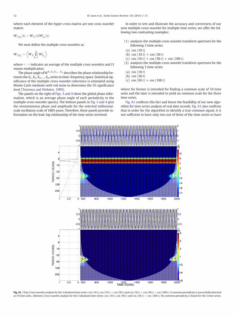
Fig. A1. (Top) Crosswavelet analysis for the 3 idealized time series: cos (10 t), cos (10 t)+cos (5at 10 time units. (Bottom) Cross wavelet analysis for the 3 idealized time series: cos (10 t), cos

In order to test and illustrate the accuracy and correctness of ournew multiple-cross-wavelet for multiple time series, we offer the fol-lowing two contrasting examples:

(1) analyzes the multiple-cross wavelet transform spectrum for thefollowing 3 time series

(a) cos (10 t)(b) cos (10 t) + cos (50 t)(c) cos (10 t) + cos (50 t) + cos (100 t)(2) analyzes the multiple-cross wavelet transform spectrum for the

following 3 time series

(a) cos (10 t)(b) cos (50 t)(c) cos (50 t) + cos (100 t)

where for former is intended for finding a common scale of 10 timeunits and the later is intended to yield no common scale for the threetime series.

Fig. A1 confirms this fact and hence the feasibility of our new algo-rithm for time series analysis of real data records. Fig. A1 also confirmsthat in order for the algorithm to identify a true common signal, it isnot sufficient to have only two out of three of the time series to have

0 t) and cos (10 t)+ cos (50 t)+cos (100 t). A commonperiodicity is successfully detected(50 t) and cos (50 t) + cos (100 t). No common periodicity is found for the 3 time series.

13W. Soon et al. / Earth-Science Reviews 134 (2014) 1–15

the common scale, i.e., the 50 time units was not picked up in the finalcross wavelet of the 3-time series.

Finally, we wish to explain and clarify that more details about themathematics of our new algorithm will be fully spelled out in a futurepaper that focuses on methodology rather than application as intendedin the current paper. Here we simply wish to state that there is simplyno clear nor direct way to inter-compare this study with any previousmethods (especially those based on Fourier transform) because no pre-vious analysis has simultaneously cross-correlated information on botha time and frequency basis for multiple (N2) time series. This is the rea-son why we have chosen to illustrate the nature of our new algorithmwith the simple example demonstrated in Fig. A1.

References

Abreu, J.A., Beer, J., Ferriz-Mas, A., McCracken, K.G., Steinhilber, F., 2012. Is there a plane-tary influence on solar activity? Astron. Astrophys. 548, A88.

Andrews, J.T., 2009. Seeking a Holocene drift ice proxy: non-clay mineral variations fromthe SW to N-central Iceland shelf: Trends, regime shifts, and periodicities. J. Quat. Sci.24, 664–676.

Andrews, J.T., Darby, D., Eberle, D., Jennings, A.E., Moros, M., Ogilvie, A., 2009. A robust,multisite Holocene history of drift ice off northern Iceland: Implications for NorthAtlantic climate. The Holocene 19, 71–77.

Arz, H.W., Gerhardt, S., Patzold, J., Rohl, U., 2001. Millennial-scale changes of surface- anddeep-water flow in the western tropical Atlantic linked to Northern Hemispherehigh-latitude climate during the Holocene. Geology 29, 239–242.

Asmerom, Y., Polyak, V., Burns, S., Rassmussen, J., 2007. Solar forcing of Holocene climate:new insights from a speleothem record, southwestern United States. Geology 35, 1–4.

Baker, P.A., Fritz, S.C., Garland, J., Ekdahl, E., 2005. Holocene hydrologic variation atLake Titicaca, Bolivia/Peru, and its relationship to North Atlantic climate variation.J. Quat. Sci. 20, 655–662.

Berger, A., Loutre, M.E., 1991. Insolation values for the climate of the last 10 million years.Quat. Sci. Rev. 10, 297–317.

Bianchi, G.G., McCave, I.N., 1999. Holocene periodicity in North Atlantic climate and deep-ocean flow south of Iceland. Nature 397, 515–517.

Bond, G., Kromer, B., Beer, J., Muscheler, R., Evans, M.N., Showers, W., Hoffmann, S., Lotti-Bond, R., Hajdas, I., Bonani, G., 2001. Persistent solar influence on North Atlanticclimate during the Holocene. Science 294, 2130–2136.

Brandenburg, A., Spiegel, E.A., 2008. Modeling a Maunder minimum. Astron. Nachr. 329,351–358.

Bray, J.R., 1968. Glaciation and solar activity since the fifth century BC and the solar cycle.Nature 220, 672–674.

Bray, J.R., 1971. Solar-climate relationships in the post-Pleistocene. Science 171,1242–1243.

Bray, J.R., 1972. Cyclic temperature oscillations from 0–20,300 yr BP. Nature 237,277–279.

Campbell, I.D., Campbell, C., Apps, M.J., Rutter, N.W., Bush, A.B.G., 1998. Late Holocene1500 yr climatic periodicities and their implications. Geology 26, 471–473.

Chapman, M.R., Shackleton, N.J., 2000. Evidence of 550-year and 1000-year cyclicitiesin North Atlantic circulation patterns during the Holocene. The Holocene 10,287–291.

Clemens, S.C., 2005. Millennial-band climate spectrum resolved and linked to centennial-scale solar cycles. Quat. Sci. Rev. 24, 521–531.

Cleroux, C., Debret, M., Cortijio, E., Duplessy, J.-C., Dewilde, F., Reijmer, J., Massei, N., 2012.High-resolution sea surface reconstructions off Cape Hatteras over the last 10 ka.Paleoceanography 27. http://dx.doi.org/10.1029/2011PA002184.

Crosta, X., Debret, M., Denis, D., Courty, M.A., Ther, O., 2007. Holocene long- and short-term climate changes off Adelie Land, East Antarctica. Geochem. Geophys. Geosyst.8. http://dx.doi.org/10.1029/2007GC001718.

Damon, P.E., Jirikowic, J.L., 1992. The Sun as a low-frequency harmonic oscillator. Radio-carbon 34, 199–205.

Darby, D.A., Ortiz, J.D., Grosch, C.E., Lund, S.P., 2012. 1,500-year cycle in the Arctic Oscilla-tion identified in Holocene Arctic sea-ice drift. Nat. Geosci. 5, 897–900. http://dx.doi.org/10.1038/NGEO1629.

de Rop, W., 1971. A tidal period of 1800 years. Tellus 23, 261–262.Debret, M., Bout-Roumazeilles, V., Grousset, F., Desmet, M., McManus, J.F., Massei, N.,

Sebag, D., Petit, J.-R., Copard, Y., Trentesaux, A., 2007. The origin of the 1500-year cli-mate cycles in Holocene North-Atlantic records. Clim. Past 3, 569–575.

Debret, M., Sebag, D., Crosta, X., Massei, N., Petit, J.-R., Chapron, E., Bout-Roumazeilles, V.,2009. Evidence from wavelet analysis for a mid-Holocene transition in a global cli-mate forcing. Quat. Sci. Rev. 28, 2675–2688.

deMenocal, P., Ortiz, J., Guilderson, T., Sarnthein, M., 2000. Coherent high- and low-latitudeclimate variability during the Holocene warm period. Science 288, 2198–2202.

Denton, G.H., Broecker, W.S., 2008. Wobbly ocean conveyor circulation during theHolocene? Quat. Sci. Rev. 27, 1939–1950.

Denton, G.H., Karlen, W., 1973. Holocene climatic variations—their pattern and possiblecause. Quat. Res. 3, 155–205.

Dima, M., Lohmann, G., 2009. Conceptual model for millennial climate variability: a pos-sible combined solar-thermohaline circulation origin for the 1500-year cycle. Clim.Dyn. 32, 301–311.

Ditlevsen, P.D., Kristensen, M.S., Andersen, K.K., 2005. The recurrence time of Dansgaard–Oeschger events and limits on the possible periodic component. J. Clim. 18,2594–2603.

Ditlevsen, P.D., Andersen, K.K., Svensson, A., 2007. The DO-climate events are probablynoise induced: statistical investigation of the claimed 1470 years cycle. Clim. Past 3,129–134.

Dixit, Y., Hodell, D.A., Petrie, C.A., 2014. Abrupt weakening of the summer monsoonin northwest India 4100 yr ago. Geology. http://dx.doi.org/10.1130/G35236.1 (inpress).

Ekdahl, E.J., Fritz, S.C., Baker, P.A., Rigsby, C.A., Coley, K., 2008. Holocene multidecadal-to millennial-scale hydrologic variability on the South American Altiplano. TheHolocene 18, 867–876.

Essex, C., 2011. Climate theory versus a theory for climate. Int. J. Bifurcation Chaos 21,3477–3487.

Essex, C., 2013. Does laboratory-scale physics obstruct the development of a theory forclimate? J. Geophys. Res. 118. http://dx.doi.org/10.1029/jgrd.50195.

Farge, M., 1992.Wavelet transforms and their applications to turbulence. Annu. Rev. FluidMech. 24, 395–457.

Fensterer, C., Scholz, D., Hoffmann, D.L., Spotl, C., Schroder-Ritzrau, A., Horn, C., Pajon, J.M.,Mangini, A., 2013. Millennial-scale climate variability during the last 12.5 ka recordedin a Caribbean speleothem. Earth Planet. Sci. Lett. 361, 143–151.

Fleitmann, D., Burns, S.J., Mudelsee, M., Neff, U., Kramers, J., Mangini, A., Matter, A., 2003.Holocene forcing of the Indian monsoon recorded in a stalagmite from SouthernOman. Science 300, 1737–1739.

Fletcher, W.J., Debret, M., Sanche Goni, M.F., 2013. Mid-Holocene emergence of a low-frequency millennial oscillation in western Mediterranean climate: implications forpast dynamics of the North Atlantic atmospheric westerlies. The Holocene 23,153–166. http://dx.doi.org/10.1177/0959683612460783.

Franco, D.R., Hinnov, L.A., Ernesto, M., 2012. Millennial-scale climate cycles in Permian-Carboniferous rhythmites: permanent feature throughout geologic time? Geology40, 19–22.

Frick, P., Baliunas, S., Galyagin, D., Sokoloff, Soon, W., 1997. Wavelet analysis of stellarchromospheric activity variations. Astrophys. J. 483, 426–434.

Giraudeau, J., Cremer, M., Manthe, S., Labeyrie, L., Bond, G., 2000. Coccolith evidence forinstabilities in surface circulation south of Iceland during Holocene times. EarthPlanet. Sci. Lett. 179, 257–268.

Giraudeau, J., Grelaud, M., Solignac, S., Andrews, J.T., Moros, M., Jansen, E., 2010.Millennial-scale variability in Atlantic water advection to the Nordic Seas derivedfrom Holocene coccolith concentration records. Quat. Sci. Rev. 29, 1276–1287.

Goni, M.A., Aceves, H., Benitez-Nelson, B., Tappa, E., Thunell, R., Black, D.E., Muller-Karger,F., Astror, Y., Valera, R., 2009. Oceanographic and climatologic controls on the compo-sitions and fluxes of biogenic materials in the water column and sediments of theCarico Basin over the late Holocene. Deep Sea Res. I 56, 614–640.

Gough, D.O., 1990. On possible origins of relatively short-term variations in the solarstructure. Philos. Trans. R. Soc. Lond. A330, 627–640.

Gough, D.O., 2002. How is solar activity influencing the structure of the Sun? From SolarMin to Max: Half a Solar Cycle with SOHO, Proceedings of SOHO 11 Symposium,(European Space Agency SP-508), pp. 577–592.

Gupta, A.K., Anderson, D.M., Overpeck, J.T., 2003. Abrupt changes in the Asian southwestmonsoon during the Holocene and their links to the North Atlantic Ocean. Nature421, 354–357.

Gupta, A.K., Das, M., Anderson, D.M., 2005. Solar influence on the Indian summer mon-soon during the Holocene. Geophys. Res. Lett. 32. http://dx.doi.org/10.1029/2005GL022685.

Hanslmeier, A., Brajsa, R., Calogovic, J., Vrsnak, B., Ruzdjak, D., Steinhilber, F., MacLeod, C.L.,Ivezic, Z., Skokic, Z.H., 2013. The chaotic solar cycle II. Analysis of cosmogenic 10Bedata. Astron. Astrophys. 550, A6.

Helama, S., Fauria, M.M., Mielikainen, K., Timonen, M., Eronen, M., 2010. Sub-Milankovitch solar forcing of past climates: mid and late Holocene perspectives.Geol. Soc. Am. Bull. 122, 1981–1988.

Hu, F.S., Kaufman, D., Yoneji, S., Nelson, D., Shemesh, A., Huang, Y., Tian, J., Bond, G., Clegg,B., Brown, T., 2003. Cyclic variation and solar forcing of Holocene climate in theAlaskan subarctic. Science 301, 1890–1893.

Hudgins, L., Friehe, C.A., Mayer, M.E., 1993. Wavelet transforms and atmospheric turbu-lence. Phys. Rev. Lett. 71, 3279–3282.

Isono, D., Yamamoto, M., Irino, T., Oba, T., Murayama, M., Nakamura, T., Kawahata, H.,2009. The 1500-year climate oscillation in the midlatitude North Pacific during theHolocene. Geology 37, 591–594.

Jackson, M.G., Oskarsson, N., Tronnes, R.G., McManus, J.F., Oppo, D.W., Gronvold, K., Hart,S.R., Sachs, J.P., 2005. Holocene loess deposition in Iceland: evidence for millennialscale atmosphere–ocean coupling in the North Atlantic. Geology 33, 509–512.

Jian, Z., Wang, P., Saito, Y., Wang, J., Pflaumann, U., Oba, T., Cheng, X., 2000. Holocene var-iability of the Kuroshio Current in the Okinawa Trough, northwestern Pacific Ocean.Earth Planet. Sci. Lett. 184, 305–319.

Jin, H., Jian, Z., 2013. Millennial-scale climate variability during the mid-Pleistocene tran-sition period in the northern South China Sea. Quat. Sci. Rev. 70, 15–27.

Johnsen, S.J., Dansgaard, W., Clausen, H.B., Langway, C.C., 1972. Oxygen isotope profilesthrough the Antarctic and Greenland ice sheets. Nature 235, 429–434.

Kanda, S., 1933. Ancient records of sunspots and auroras in the Far East and the variationof the period of solar activity. Proc. Imp. Acad. 9, 293–296.

Kao, S.J., Horng, C.S., Hsu, S.C., Wei, K.Y., Chen, J., Lin, Y.S., 2005. Enhanced deepwater cir-culation and shift of sedimentary organic matter oxidation pathway in the OkinawaTrough since the Holocene. Geophys. Res. Lett. 32, L15609. http://dx.doi.org/10.1029/2005GL023139.

Keeling, C.D., Whorf, T.P., 2000. The 1800-year oceanic tidal cycle: a possible cause ofrapid climate change. Proc. Natl. Acad. Sci. U. S. A. 97, 3814–3819.

14 W. Soon et al. / Earth-Science Reviews 134 (2014) 1–15

Kemp, J., Radke, L.C., Olley, J., Juggins, S., de Deckker, P., 2012. Holocene lake salinitychanges in the Wimmera, southeastern Australia, provide evidence for millennial-scale climate variability. Quat. Res. 77, 65–76.

Kern, A.K., Harzhauser, M., Piller, W.E., Mandic, O., Soliman, A., 2012. Strong evidence forthe influence of solar cycles on a Late Miocene lake system revealed by biotic andabiotic proxies. Palaeogeogr. Palaeoclimatol. Palaeoecol. 329–330, 124–136.

Kim, J.-H., Rimbu, N., Lorenz, S.J., Lohmann, G., Nam, S.-I., Schouten, S., Ruhlemann, C.,Schneider, R.R., 2004. North Pacific and North Atlantic sea-surface temperature vari-ability during the Holocene. Quat. Sci. Rev. 23, 2141–2154.

Konecky, B.L., Russell, J.M., Rodysill, J.R., Vuille, M., Bijaksana, S., Huang, Y., 2013. Intensi-fication of southwestern Indonesian rainfall over the past millennium. Geophys. Res.Lett. 40, 386–391. http://dx.doi.org/10.1029/2012GL054331.

Kravchinsky, V.A., Langereis, C.G., Walker, S.D., Dlusskiy, K.G., White, D., 2013. Discoveryof Holocene millennial climate cycles in the Asian continental interior: has the sunbeen governing the continental climate? Global Planet. Change 110, 386–396.http://dx.doi.org/10.1016/j.gloplacha.2013.02.011.

Laluraj, C.M., Thamban, M., Naik, S.S., Redkar, B.L., Chaturvedi, A., Ravindra, R., 2011.Nitrate records of a shallow ice core from East Antarctica: atmospheric processes,preservation and climatic implications. The Holocene 21, 351–356.

Lim, J., Yi, S., Nahm, W.-H., Kim, J.-Y., 2012. Holocene millennial-scale vegetation changesin the Yugu floodplain, Kongju area, central South Korea. Quat. Int. 254, 92–98.

Lim, J., Nahm, W.-H., Kim, J.-Y., Yang, D.-Y., 2013. Reply to comment on “” by J. Lim, W.-H.,Nahm, J.-K., Kim, D.-Y., Yang [Palaeogeography, Palaeoclimatology, Palaeoecology 298(2010) 370–377]. Palaeogeogr. Palaeoclimatol. Palaeoecol. 392, 559–561. http://dx.doi.org/10.1016/j.palaeo.2013.08.004.

Lou, J.Y., Chen, C.T.A., 1997. Paleoclimatological and paleoenvironmental records since4000 a B.P. in the sediments of alpine lakes in Taiwan. Sci. China D Earth Sci. 40,424–431.

Mackay, A.W., Swann, G.E.A., Fagel, N., Fietz, S., Leng, M.J., Morley, D., Rioual, P., Tarasov, P.,2013. Hydrological instability during the Last Interglacial in central Asia: a newdiatom oxygen isotope record from Lake Baikal. Quat. Sci. Rev. 66, 45–54.

Marchitto, T.M., deMenocal, P.B., 2003. Late Holocene variability of upper North Atlanticdeep water temperature and salinity. Geochem. Geophys. Geosyst. 4. http://dx.doi.org/10.1029/2003GC000598.

Marchitto, T.M., Muscheler, R., Ortiz, J.D., Carriquiry, J.D., van Geen, A., 2010. Dynamicalresponse of the tropical Pacific Ocean to solar forcing during the early Holocene.Science 330, 1378–1381.

Markonis, Y., Koutsoyiannis, D., 2013. Climatic variability over time scales spanning nineorders of magnitude: connecting Milankovitch cycles with Hurst–Kolmogorov dy-namics. Surv. Geophys. 34, 181–207. http://dx.doi.org/10.1007/s10712-012-9208-9.

Mayewski, P.A., Meeker, L.D., Twickler, M.S., Whitlow, S., Yang, Q., Lyons, W.B., Prentice,M., 1997. Major features and forcing of high-latitude northern hemisphere atmo-spheric circulation using a 110,000-year-long glaciochemical series. J. Geophys. Res.102, 26345–26366. http://dx.doi.org/10.1029/96JC03365.

Mayewski, P.A., Rohling, E.E., Stager, J.C., Karlen, W., Maasch, K.A., Meeker, L.D., Meyerson,E.A., Gasse, F., van Kreveld, S., Holmgren, K., Lee-Thorp, J., Rosqvist, G., Rack, F.,Staubwasser, M., Schneider, R.R., Steig, E.J., 2004. Holocene climatic variability. Quat.Res. 62, 243–255.

McCracken, K.G., Dreschhoff, G.A.M., Zeller, E.J., Smart, D.F., Shea, M.A., 2001. Solar cosmicray events for the period 1561–994: 1. Identification in polar ice, 1561–1950. J.Geophys. Res. 106. http://dx.doi.org/10.1029/2000JA000237.

McDermott, F., Mattey, D.P., Hawkesworth, C., 2001. Centennial-scale Holocene climatevariability revealed by a high-resolution speleothem δ18O record from SW Ireland.Science 294, 1328–1331 ([with erratum printed 16 September 2005]).

Morley, A., Schulz, M., Rosenthal, Y., Mulitza, S., Paul, A., Ruhlemann, C., 2011. Solar mod-ulation of North Atlantic central water formation at multidecadal timescales duringthe late Holocene. Earth Planet. Sci. Lett. 308, 161–171.

Moros, M., Emeis, K., Risebrobakken, B., Snowball, I., Kuijpers, A., McManus, J., Jansen, E.,2004. Sea surface temperatures and ice rafting in the Holocene North Atlantic: cli-mate influences on northern Europe and Greenland. Quat. Sci. Rev. 23, 2113–2126.

Moros, M., Deckker, P.D., Jansen, E., Perner, K., Telford, R.J., 2009. Holocene climate vari-ability in the Southern Ocean recorded in a deep-sea sediment core off SouthAustralia. Quat. Sci. Rev. 28, 1932–1940.

Moy, C.M., Seltzer, G.O., Rodbell, D.T., Anderson, D.M., 2002. Variability of El Nino/Southern Oscillation activity at millennial timescales during the Holocene epoch.Nature 420, 162–165.

Munk,W., Dzieciuch, M., Jayne, S., 2002. Millennial climate variability: is there a tidal con-nection? J. Clim. 15, 370–385.

Naidu, P.D., Malmgren, B.A., 1995. A 2,200 years periodicity in the Asianmonsoon system.Geophys. Res. Lett. 22, 2361–2364. http://dx.doi.org/10.1029/95GL02558.

Nielsen, S.H.H., Koc, N., Crosta, X., 2004. Holocene climate in the Atlantic sector of theSouthern Ocean controlled by insolation or oceanic circulation? Geology 32, 317–320.

Noren, A.J., Bierman, P.R., Steig, E.J., Lini, A., Southon, J., 2002. Millennial-scale storminessvariability in the northeastern United States during the Holocene epoch. Nature 419,821–824.

O'Brien, S.R., Mayewski, P.A., Meeker, L.D., Meese, D.A., Twickler, M.S., Whitlow, S.I., 1995.Complexity of Holocene climate as reconstructed from a Greenland ice core. Science270, 1962–1964.

Obrochta, S.P., Miyahara, H., Yokoyama, Y., Crowley, T.J., 2012. A re-examination of evi-dence for the North Atlantic “1500-year cycle” at Site 609. Quat. Sci. Rev. 55, 23–33.

Ogurtsov, M.G., Oinonen, M., 2014. Evidence of the solar Gleissberg cycle in the nitrateconcentration in polar ice. J. Atmos. Sol. Terr. Phys. 109, 37–42.

Panovska, S., Finlay, C.C., Hirt, A.M., 2013. Observed periodicities and the spectrum of fieldvariations in Holocene magnetic records. Earth Planet. Sci. Lett. 373, 88–94.

Park, W., Latif, M., 2012. Atlantic meridional overturning circulation response to idealizedexternal forcing. Clim. Dyn. 39, 1709–1726.

Pena, L.D., Frances, G., Diz, P., Esparza, M., Grimalt, J.O., Nombela, M.A., Alejo, I., 2010. Cli-mate fluctuations during the Holocene in NW Iberia: High and low latitude linkages.Cont. Shelf Res. 30, 1487–1496.

Peristykh, A.N., Damon, P.E., 2003. Persistence of the Gleissberg 88-year solar cycle overthe last 12,000 years: evidence from cosmogenic isotopes. J. Geophys. Res. 108.http://dx.doi.org/10.1029/2002JA009390.

Perry, C.A., Hsu, K.J., 2000. Geophysical, archaeological, and historical evidence support asolar-output model for climate change. Proc. Natl. Acad. Sci. U. S. A. 97, 12433–12438.

Petersen, S.V., Schrag, D.P., Clark, P.U., 2013. A new mechanism for Dansgaard–Oeschgercycles. Paleoceanography 28, 24–30. http://dx.doi.org/10.1029/2012PA002364.

Pipin, V.V., 1999. The Gleissberg cycle by a nonlinear αΛ dynamo. Astron. Astrophys. 346,295–302.

Pipin, V.V., Sokoloff, D.D., Usoskin, I.G., 2012. Variations of the solar cycle profile in a solardynamo with fluctuating dynamo governing parameters. Astron. Astrophys. 542, A26.

Pipin, V.V., Sokoloff, D.D., Usoskin, I.G., 2013. Waldmeier relations and the solar cycle dy-namics by the mean-field dynamos. In: Kosovichev, A.G., de Gouveia Dal Pinto, E.M.,Yan, Y. (Eds.), Solar and Astrophysical Dynamos and Magnetic Activity (IAU Sympo-sium No. 294) ([available at http://arxiv.org/abs/1211.2423]).

Pisias, N.G., Clark, P.U., Brook, E.J., 2010. Modes of global climate variability during MarineIsotope Stage 3 (60–26 ka). J. Clim. 23, 1581–1588.

Prasad, S., Anoop, A., Riedel, N., Sarkar, S., Menzel, P., Basavaiah, N., Krishnan, R., Fuller, D.,Plessen, B., Gaye, B., Rohl, U., Wilkes, H., Sachse, D., Sawant, R., Wiesner, M.G., Stebich,M., 2014. Prolonged monsoon droughts and links to Indo-Pacific warm pool: aHolocene record from Lonar Lake, central India. Earth Planet. Sci. Lett. 391, 171–182.

Risebrobakken, B., Jansen, E., Anderson, C., Mjelde, E., Hevroy, K., 2003. Solar forcing ofFlorida Straits surface salinity during the early Holocene. Paleoceanography 18.http://dx.doi.org/10.1029/2002PA000764.

Rosqvist, G., Schuber, P., 2003. Millennial-scale climate changes on South Georgia, South-ern Ocean. Quat. Res. 59, 470–475.

Santos, T.P., Franco, D.R., Barbosa, C.F., Belem, A.L., Dokken, T., Albuquerque, A.L.S., 2013.Millennial- to centennial-scale changes in sea surface temperature in the tropicalSouth Atlantic throughout the Holocene. Palaeogeogr. Palaeoclimatol. Palaeoecol.392, 1–8. http://dx.doi.org/10.1016/j.palaeo.2013.08.019.

Sarkar, A., Ramesh, R., Somayajulu, B.L.K., Agnihotri, R., Jull, A.J.T., Burr, G.S., 2000. Highresolution Holocene monsoon record from the eastern Arabian Sea. Earth Planet.Sci. Lett. 177, 209–218.

Savarino, J., Kaiser, J., Morin, S., Sigman, D.M., Thiemens, M.H., 2007. Nitrogen and oxygenisotopic constraints on the origin of atmospheric nitrate in coastal Antarctica. Atmos.Chem. Phys. 7, 1925–1945.

Schmidt, M.W., Weinlein, W.A., Marcantonio, F., Lynch-Stieglitz, J., 2012. Solar forcing ofFlorida Straits surface salinity during the early Holocene. Paleoceanography 27.http://dx.doi.org/10.1029/2012PA002284.

Schulz, M., 2002. On the 1470-year pacing of Dansgaard–Oeschger warm events.Paleoceanography 17. http://dx.doi.org/10.1029/2000PA000571.

Schulz, M., Berger, W.H., Sarnthein, M., Grootes, P.M., 1999. Amplitude variations of 1470-year climate oscillations during the last 100,000 years linked to fluctuations of conti-nental ice mass. Geophys. Res. Lett. 26, 3385–3388. http://dx.doi.org/10.1029/1999GL006069.

Seidenglanz, A., Prange, M., Varma, V., Schulz, M., 2012. Ocean temperature response toidealized Gleissberg and de Vries solar cycles in a comprehensive climate model.Geophys. Res. Lett. 39. http://dx.doi.org/10.1029/2012GL053624.

Selvaraj, K., Chen, C.-T.A., Lou, J.-Y., 2007. Holocene East Asian monsoon variability: linksto solar and tropical Pacific forcing. Geophys. Res. Lett. 34. http://dx.doi.org/10.1029/2006GL028155.

Selvaraj, K., Chen, C.-T.A., Lou, J.-Y., Kotlia, B.S., 2011. Holocene weak summer East Asianmonsoon intervals in Taiwan and plausible mechanisms. Quat. Int. 229, 57–66.

Sirocko, F., Garbe-Schonberg, D., McIntyre, A., Molfino, B., 1996. Teleconnections betweensubtropical monsoons and high-latitude climates during the last deglaciation. Science272, 526–529.

Soon, W., 2009. Solar Arctic-mediated climate variation on multidecadal to centennialtimescales: empirical evidence, mechanistic explanation, and testable consequences.Phys. Geogr. 30, 144–184.

Soon, W., Legates, D.R., 2013. Solar irradiance modulation of equator-to-pole (Arctic)temperature gradients: empirical evidence for climate variation on multidecadaltimescales. J. Atmos. Sol. Terr. Phys. 93, 45–56.

Soon, W., Frick, P., Baliunas, S., 1999. Lifetime of surface features and stellar rotation: awavelet time–frequency approach. Astrophys. J. Lett. 510, L135–L138.

Soon,W., Dutta, K., Legates, D.R., Velasco, V., Zhang,W., 2011. Variation in surface air tem-perature of China during the 20th Century. J. Atmos. Sol. Terr. Phys. 73, 2331–2344.

Sorrel, P., Debret, M., Billeaud, I., Jaccard, S.L., McManus, J.F., Tessier, B., 2012. Persistentnon-solar forcing of Holocene storm dynamics in coastal sedimentary archives. Nat.Geosci. 5, 892–896. http://dx.doi.org/10.1038/NGEO1619.

Spiegel, E.A., 2009. Chaos and intermittency in the solar cycle. Space Sci. Rev. 144, 25–51.Stenni, B., Proposito, M., Gragnani, R., Flora, O., Jouzel, J., Falourd, S., Frezzotti, M., 2002.

Eight centuries of volcanic signal and climate change at Talos Dome (EastAntarctica). J. Geophys. Res. 107. http://dx.doi.org/10.1029/2000JD000317.

St-Onge, G., Stoner, J.S., Hillaire-Marcel, C., 2003. Holocene paleomagnetic records fromthe St. Lawrence estuary, eastern Canada: Centennial- to millennial-scale geomagnet-ic modulation of cosmogenic isotopes. Earth Planet. Sci. Lett. 209, 113–130.

Stott, L., Cannariato, K., Thunell, R., Haug, G.H., Koutavas, A., Lund, S., 2004. Decline of sur-face temperature and salinity in the western tropical Pacific Ocean in the Holoceneepoch. Nature 431, 56–59.

Strikis, N.M., Cruz, F.W., Cheng, H., Karmann, I., Edwards, R.L., Vuille, M., Wang, X., dePaula, M.S., Novello, V.F., Auler, A.S., 2011. Abrupt variations in South American mon-soon rainfall during the Holocene based on a speleothem record from central-easternBrazil. Geology 39, 1075–1078.

15W. Soon et al. / Earth-Science Reviews 134 (2014) 1–15

Stuiver, M., Grootes, P.M., Braziunas, T.F., 1995. The GISP2 δ18O climate record of the past16,500 years and the role of the Sun, ocean and volcanoes. Quat. Res. 44, 341–354.

Thamban, M., Kawahata, H., Rao, V.P., 2007. Indian summer monsoon variability duringthe Holocene as recorded in sediments of the Arabian Sea: timing and implications.J. Oceanogr. 63, 1009–1020.

Thompson, L.G., Mosley-Thompson, E., Davis, M.E., Lin, P.-N., Henderson, K.A., Cole-Dai, J.,Bolzan, J.F., Liu, K.-B., 1995. Late glacial stage and Holocene tropical ice core recordsfrom Huascaran, Peru. Science 269, 46–50.

Thompson, L.G., Davis, M.E., Mosley-Thompson, E., Sowers, T.A., Henderson, K.A.,Zagorodnov, V.S., Lin, P.-N., Mikhalenko, V.N., Campen, R.K., Bolzan, J.F., Cole-Dai, J.,Francou, B., 1998. A 25,000-year tropical climate history from Bolivian ice cores.Science 282, 1858–1864.

Thornalley, D.J.R., Elderfield, H., McCave, I.N., 2009. Holocene oscillations in temperatureand salinity of the subpolar North Atlantic. Nature 457, 711–714.

Tobias, S.M., Weiss, N.O., 2000. Resonant interactions between solar activity and climate.J. Clim. 13, 3745–3759.

Torrence, C., Compo, G., 1998. A practical guide to wavelet analysis. Bull. Am. Meteorol.Soc. 79, 61–78.

Torrence, C., Webster, P., 1999. Interdecadal changes in ENSO-Monsoon system. J. Clim.12, 2679–2690.

Traversi, R., Usoskin, I.G., Solanki, S.K., Becagli, S., Frezzotti, M., Severi, M., Stenni, B., Udisti,R., 2012. Nitrate in polar ice: a new tracer of solar variability. Sol. Phys. 280, 237–254.

Turney, C., Baillie, M., Clemens, S., Brown, D., Palmer, J., Pilcher, J., Reimer, P., Leuschner, H.H., 2005. Testing solar forcing of pervasive Holocene climate cycles. J. Quat. Sci. 20,511–518.

Usoskin, I.G., 2013. A history of solar activity over millennia. Living Rev. Sol. Phys. 10, 1(updated March 21, 2013; available at http://www.livingreviews.org/lrsp-2013-1).

Usoskin, I.G., Kromer, B., 2005. Reconstruction of the 14C production rate from measuredrelative abundance. Radiocarbon 47, 31–37.

Usoskin, I.G., Alanko-Huotari, K., Kovaltsov, G.A., Mursula, K., 2005. Heliospheric modula-tion of cosmic rays: monthly reconstruction for 1951–2004. J. Geophys. Res. 110.http://dx.doi.org/10.1029/2005JA011250.

Usoskin, I.G., Solanki, S.K., Kovaltsov, G.A., 2007. Grand minima and maxima of solaractivity: new observational constraints. Astron. Astrophys. 471, 301–309.

van Loon, H., Brown, J., Milliff, R.F., 2012. Trends in sunspots and North Atlantic sea-levelpressure. J. Geophys. Res. 117. http://dx.doi.org/10.1029/2012JD017502.

Vasiliev, S.S., Dergachev, V.A., 2002. The 2400-year cycle in atmospheric radiocarbonconcentration: bispectrum of 14C data over the last 8000 years. Ann. Geophys. 20,115–120.

Velasco Herrera, V.M., 2013. The (super)-secular periodicity of the cosmic rays during theHolocene. In: Perez-Peraza, Jorge A. (Ed.), Homage to the Discovery of Cosmic Rays, theMeson-Muon and Solar Cosmic Rays, Nova, pp. 469–476 (chapter 15).

Vonmoos, M., Beer, J., Muscheler, R., 2006. Large variations in Holocene solar activity: con-straints from 10Be in the Greenland Ice Core Project ice core. J. Geophys. Res. 111.http://dx.doi.org/10.1029/2005JA011500.

Wang, Y.J., Cheng, H., Edwards, R.L., He, Y., Kong, X., An, Z.S., Wu, J., Kelly, M.J., Dykoski, C.A., Li, X., 2005. The Holocene Asian monsoon: links to solar changes and North Atlan-tic climate. Science 308, 854–857.

Wang, Y., Li, S., Luo, D., 2009. Seasonal response of Asian monsoonal climate to theAtlantic Multidecadal Oscillation. J. Geophys. Res. 114. http://dx.doi.org/10.1029/2008JD010929.

Wanner, H., Beer, J., Butikofer, J., Crowley, T.J., Cubasch, U., Fluckiger, Goosse, H., Grosjean,M., Joos, F., Kaplan, J.O., Kuttel, M., Muller, S.A., Prentice, I.C., Solomina, O., Stocker, T.F.,Tarasov, P., Wagner, M., Widmann, M., 2008. Mid- to Late Holocene climate change:an overview. Quat. Sci. Rev. 27, 1791–1828.

Weiss, N.O., 2011. Solar and stellar dynamos. In: Brummell, N.H., Brun, A.S., Miesch, M.S.,Ponty, Y. (Eds.), Astrophysical Dynamics: From Stars to Galaxies. Proceedings of theInternational Astronomical Union, IAU symposium, vol. 271, pp. 247–260.

Weng, H., 2012a. Impact of multi-scale solar activity on climate. Part I: Atmospheric circu-lation patterns and climate extremes. Adv. Atmos. Sci. 29, 867–886.

Weng, H., 2012b. Impact of multi-scale solar activity on climate. Part II: Dominant time-scales in decadal-centennial climate variability. Adv. Atmos. Sci. 29, 887–908.

Wiener, N., 1930. Generalized harmonic analysis. Acta Math. 55, 117–258.Wilkins, D., Gouramanis, C., deDeckker, P., Fifield, L.K., Olley, J., 2013. Holocene lake-level

fluctuations in Lakes Keilambete and Gnotuk, southwestern Victoria, Australia. TheHolocene 23, 784–795. http://dx.doi.org/10.1177/0959683612471983.

Wolff, E.W., Bigler, M., Curran, M.A.J., Dibb, J.E., Frey, M.M., Legrand, M., McConnell, J.R.,2012. The Carrington event not observed in most ice core nitrate records. Geophys.Res. Lett. 39. http://dx.doi.org/10.1029/2012GL051603.

Wunsch, C., 2000. On sharp spectral lines in the climate record and the millennial peak.Paleoceanography 15, 417–424. http://dx.doi.org/10.1029/1999PA000468.

Xie, P., Vallis, G.K., 2012. The passive and active nature of ocean heat uptake in idealizedclimate change experiments. Clim. Dyn. 38, 667–684.

Yu, Y., Yang, T., Li, J., Liu, J., An, C., Liu, X., Fan, Z., Lu, Z., Li, Y., Su, X., 2006. Millennial-scaleHolocene climate variability in the NWChina drylands and links to the tropical Pacificand the North Atlantic. Palaeogeogr. Palaeoclimatol. Palaeoecol. 233, 149–162.

Zhao, C., Yu, Z., Ito, E., Zhao, Y., 2010. Holocene climate trend, variability, and shift docu-mented by lacustrine stable-isotope record in northeastern United States. Quat. Sci.Rev. 29, 1831–1843.

Zhao, C., Liu, Z., Rohling, E., Yu, Z., Liu, W., He, Y., Zhao, Y., Chen, F., 2013. Holocene tem-perature fluctuations in the northern Tibetan Plateau. Quat. Res. 80, 55–65.