Information Sciences 217 (2012) 56–64

Contents lists available at SciVerse ScienceDirect

Information Sciences

journal homepage: www.elsevier .com/locate / ins

A reduced support vector machine approach for interval regression analysis

Chia-Hui Huang ⇑Department of Business Administration, National Taipei College of Business, No. 321, Section 1, Jinan Rd., Zhongzheng District, Taipei City 100, Taiwan

a r t i c l e i n f o

Article history:Received 26 September 2011Received in revised form 4 May 2012Accepted 23 June 2012Available online 2 July 2012

Keywords:Interval regression analysisFuzzy regressionReduced support vector machine

0020-0255/$ - see front matter � 2012 Elsevier Inchttp://dx.doi.org/10.1016/j.ins.2012.06.030

⇑ Tel.: +886 2 2322 6402; fax: +886 2 2322 6404E-mail address: leohuang@webmail.ntcb.edu.tw

a b s t r a c t

The support vector machine (SVM) has been shown to be an efficient approach for a varietyof classification problems. It has also been widely used in pattern recognition, regressionand distribution estimation for separable data. However, there are two problems withusing the SVM model: (1) Large-scale: when dealing with large-scale data sets, the solutionmay be difficult to find when using SVM with nonlinear kernels; (2) Unbalance: the num-ber of samples from one class is much larger than the number of samples from the otherclasses. It causes the excursion of separation margin. Under these circumstances, develop-ing an efficient method is necessary.

Recently, the use of the reduced support vector machine (RSVM) was proposed as analternative to the standard SVM. It has been proven more efficient than the traditionalSVM in processing large-scaled data. In this paper, we introduce the principle of RSVMto evaluate interval regression analysis. The main idea of the proposed method is to reducethe number of support vectors by randomly selecting a subset of samples.

� 2012 Elsevier Inc. All rights reserved.

1. Introduction

Since Tanaka et al. [38] introduced the fuzzy regression model with symmetric fuzzy parameters, many researchers havestudied the properties of fuzzy regression extensively. A collection of recent studies to fuzzy regression analysis can be foundin [2,3,5,6,9,10,13–17,35–39].

The fuzzy regression model can be simplified to interval regression analysis, which is considered as the simplest versionof possibilistic regression analysis with interval coefficients. Some coefficients in interval linear regression models tend tobecome separable due to the characteristics of linear programming (LP) [38]. To alleviate the issue of LP, Tanaka and Lee[37] propose an interval regression analysis with a quadratic programming (QP) approach, which gives a more diverse spreadof coefficients than by using the LP approach.

The support vector machine (SVM) has been widely used in pattern recognition, regression and distribution estimation[1,4,7,8,11,12,21,23–31,33,40–42]. Arun Kumar et al. [1] incorporated prior knowledge represented by polyhedral sets intoa relatively new family of SVM classifiers based on two non-parallel hyperplanes and proposed two formulations termed asknowledge based Twin SVM (KBTWSVM) and knowledge based Least Squares Twin SVM (KBLSTWSVM), both capable of gen-erating non-parallel hyperplanes from given data and prior knowledge. Maldonado et al. [21] proposed an embedded meth-od for feature selection and classification using kernel-penalized SVM (KP-SVM). The KP-SVM simultaneously selectsrelevant features during classifier construction by penalizing each feature’s use in the dual formulation of SVM. Savithaet al. [28] developed a fast learning fully complex-valued extreme learning machine classifier, referred to as Circular Com-plex-valued Extreme Learning Machine (CC-ELM) for handling real-valued classification problems. CC-ELM classifier uses asingle hidden layer network with a non-linear input/hidden layer and a linear output layer. The results show that CC-ELM

. All rights reserved.

.

C.-H. Huang / Information Sciences 217 (2012) 56–64 57

performs better than other existing real-valued and complex-valued classifiers, especially when the data sets are highlyunbalanced. Unler et al. [40] introduced a hybrid filter-wrapper feature subset selection algorithm based on particle swarmoptimization (PSO) for SVM classification. The filter model is based on the mutual information and is a composite measure offeature relevance and redundancy with respect to the feature subset selected. The experimental results show that themr2PSO algorithm is competitive in terms of both classification accuracy and computational performance.

Recently, using SVM to solve the interval regression model has become an alternative approach. Hong and Hwang intro-duced SVM for multivariate fuzzy regression analysis [13] and evaluated interval regression models with quadratic loss SVM[14]. Jeng et al. [16] developed a support vector interval regression networks (SVIRNs) based on both SVM and neural net-works. Bisserier et al. [2] proposed a revisited fuzzy regression method where a linear model is identified from Crisp-InputsFuzzy-Outputs (CISO) data. D’Urso et al. [10] presented fuzzy clusterwise regression analysis with LR fuzzy response variableand numeric explanatory variables. The suggested model is to allow for linear and non-linear relationship between the out-put and input variables.

However, there are two problems with using the SVM model:

1. Large-scale: when dealing with large-scale data sets, the solution may be difficult to find when using SVM with nonlinearkernels.

2. Unbalance: the number of samples from one class is much larger than the number of samples from other classes. It causesthe excursion of separation margin.

Under these circumstances, developing an efficient method is necessary. The reduced support vector machine (RSVM) hasbeen proven more efficient than the traditional SVM in processing large-scaled data [18–20]. The main purpose of RSVM is toreduce the number of support vectors by randomly selecting a subset of samples. In this report, we introduce the principle ofRSVM to evaluate interval regression analysis.

This paper is organized in the following manner. Section 2 reviews interval regression analysis by the QP approach, thusunifying the possibility and necessity models. Section 3 proposes the formulation of RSVM in evaluating the interval regres-sion models. Section 4 provides the numerical examples to illustrate the methods. Finally, Section 5 presents the concludingremarks.

2. Interval regression analysis with the QP approach

In this section we review interval regression analysis by a quadratic programming (QP) approach, thus unifying the pos-sibility and necessity models proposed by Tanaka and Lee [37].

An interval linear regression model is described as

YðxjÞ ¼ A0 þ A1x1j þ � � � þ Anxnj ð1Þ

where YðxjÞ; j ¼ 1;2; . . . ; q is the estimated interval corresponding to the real input vector xj ¼ ðx1j; x2j; . . . ; xnjÞT . An intervalcoefficient Ai is defined as ðai; ciÞ; i ¼ 1;2; . . . ;n, where ai is a center and ci is a radius. Hence, Ai can also be represented as

Ai ¼ fujai � ci 6 u 6 ai þ cig ¼ ½ai � ci; ai þ ci� ð2Þ

The interval linear regression model (1) can also be expressed as

YðxjÞ ¼ A0 þ A1x1j þ � � � þ Anxnj ¼ ða0; c0Þ þ ða1; c1Þx1j þ � � � þ ðan; cnÞxnj ¼ a0 þXn

i¼1

aixij; c0 þXn

i¼1

cijxijj !

ð3Þ

For a data set with non-fuzzy inputs and interval outputs, two interval regression models, the possibility and necessity mod-els, are considered. By assumption, the center coefficients of the possibility regression model and the necessity regressionmodel are the same [37].

Assume that input–output data ðxj; YjÞ are given as

ðxj; YjÞ ¼ ð1; x1j; . . . ; xnj; YjÞ; j ¼ 1;2; . . . ; q ð4Þ

where xj is the jth input vector, Yj is the corresponding interval output that consists of a center yj and a radius ej denoted asYj ¼ ðyj; ejÞ, and q is a data size. For this data set, the possibility and necessity estimation models are defined as

Y�ðxjÞ ¼ A�0 þ A�1x1j þ � � � þ A�nxnj ð5ÞY�ðxjÞ ¼ A0� þ A1�x1j þ � � � þ An�xnj ð6Þ

where the interval coefficients A�i and Ai� are defined as A�i ¼ ða�i ; c�i Þ and Ai� ¼ ðai�; ci�Þ, respectively. The interval Y�ðxjÞ esti-mated by the possibility model must include the observed interval Yj. The interval Y�ðxjÞ estimated by the necessity modelmust also be included in the observed interval Yj. The following inclusion relations exist

Y�ðxjÞ# Yj # Y�ðxjÞ ð7Þ

The interval coefficients A�i and A�i can be denoted as

58 C.-H. Huang / Information Sciences 217 (2012) 56–64

A�i ¼ ðai; ci þ diÞ ð8ÞAi� ¼ ðai; ciÞ ð9Þ

which satisfy the inclusion relation Ai�# A�i where ci and di are assumed to be positive. Thus, the possibility model Y�ðxjÞ andthe necessity model Y�ðxjÞ can also be expressed as

Y�ðxjÞ ¼ a0 þXn

i¼1

aixij; c0 þXn

i¼1

cijxijj þ d0 þXn

i¼1

dijxijj !

ð10Þ

Y�ðxjÞ ¼ a0 þXn

i¼1

aixij; c0 þXn

i¼1

cijxijj !

ð11Þ

The interval regression analysis by the QP approach unifying the possibility and necessity models subject to the inclusionrelations Y�ðxjÞ# Yj # Y�ðxjÞ can then be represented as

minXq

j¼1

d0 þXn

i¼1

dijxijj !2

þuXn

i¼0

ða2i þ c2

i Þ

s:t:

Y�ðxjÞ# Yj # Y�ðxjÞ; j ¼ 1;2; . . . ; q

ci;di P 0; i ¼ 0;1; . . . ;n

ð12Þ

where u is an extremely small positive number and makes the influence of the term uPn

i¼0ða2i þ c2

i Þ in the objective functionnegligible. The constraints of the inclusion relations are equivalent to

Y�ðxjÞ# Yj ()

yj � ej 6 a0 þXn

i¼1

aixij

!� c0 þ

Xn

i¼1

cijxijj !

ða0 þXn

i¼1

aixijÞ þ c0 þXn

i¼1

cijxijj !

6 yj þ ej

8>>>>><>>>>>:

ð13Þ

Yj # Y�ðxjÞ ()

ða0 þXn

i¼1

aixijÞ � ðc0 þXn

i¼1

cijxijjÞ � d0 þXn

i¼1

dijxijj !

6 yj � ej

yj þ ej 6 a0 þXn

i¼1

aixij

!þ c0 þ

Xn

i¼1

cijxijj !

þ ðd0 þXn

i¼1

dijxijjÞ

8>>>>><>>>>>:

ð14Þ

where xj is the jth input vector, Yj is the corresponding interval output that consists of a center yj and a radius ej denoted asYj ¼ ðyj; ejÞ, and q is a data size.

3. Proposed methods

In this section, we introduce a new method to evaluate interval linear and nonlinear regression models associated withthe possibility and necessity formulation using the principle of a reduced support vector machine.

We first briefly introduce the basis of the theory of the reduced support vector machine (RSVM) [18,19]. Suppose that ntraining data fxi; yig; i ¼ 1;2; . . . ;n are given, where xi 2 Rn are the input patterns and yi are the related target values of a two-class pattern classification case. This setting distinguishes two categories of data. Then, the standard support vector machinewith a linear kernel [41,42] is

minw;b;n

12kwk2 þ C

Xn

i¼1

ni þ n�i

!

s:t:

yi �wT xi � b 6 eþ ni

wT xi þ b� yi 6 eþ n�ini; n

�i P 0; i ¼ 1;2; . . . ; n

ð15Þ

where b is the location of the hyperplane relative to the origin, the regularization constant C > 0 is the penalty parameter ofthe error term used to determine the tradeoff between the flatness of linear functions ðwT xi þ bÞ and the amount up to whichdeviations larger than e are tolerated, ni and n�i are the slack variables, and kwk is the Euclidean norm of w.

In [18–20], b2=2 is added to the objective function of (15). This is equivalent to adding a constant feature to the training

data and finding a separating hyperplane through the origin.

C.-H. Huang / Information Sciences 217 (2012) 56–64 59

minw;b;n

12ðkwk2 þ b2Þ þ C

Xn

i¼1

ni þ n�i

!

s:t:

yi �wT xi � b 6 eþ ni

wT xi þ b� yi 6 eþ n�ini P 0; i ¼ 1;2; . . . ;n

ð16Þ

Its dual becomes the following bound-constrained problem [18–20]

mina

12aT Q þ I

2Cþ yT y

� �a� �Ta

s:t:

0 6 ai; i ¼ 1;2; . . . ;n

ð17Þ

where a is the vector of the corresponding coefficients, � is the vector of all ones, Qij � yiyjKðxi; xjÞ is a positive semi-definitematrix, and Kðxi; xjÞ is the kernel function. In this case, Kðxi; xjÞ � xT

i xj is a linear kernel.In the optimal solution, w ¼

Pni¼1yiaixi is a linear combination of training data. Substituting w into (16),

yiwT xi ¼

Xn

j¼1

yiyjajxTj xi ¼

Xn

j¼1

Qijaj ¼ ðQaÞi ð18Þ

kwk2 ¼Xn

i¼1

yiaixTi w ¼

Xn

j¼1

aiðQaÞi ¼ aT Qa ð19Þ

The problem becomes

mina;b;n

12ðaT Qaþ b2Þ þ C

Xn

i¼1

ni þ n�i

!

s:t:

Qaþ by P �� n

ð20Þ

Dealing with large-scale data sets, the main idea of RSVM is to reduce the number of support vectors by randomly selecting asubset of k samples for w

w ¼Xi2K

yiaixi ð21Þ

where K contains indices of the subset of k samples. The problem becomes (22) by substituting (21) with the number of ma-jor variables reduced to k

min�a;b;n

12ð�aT Q K;K �aþ b2Þ þ C

Xn

i¼1

ni þ n�i

!

s:t:

Q �;K �aþ by P �� n

ð22Þ

where �aK is the collection of all ai; i 2 K. Q �;K represents the sub-matrix of columns corresponding to K.To simplify the term 1=2ð�aT Q K;K �aÞ to 1=2ð�aT �aÞ following the generalized support vector machine (GSVM) by Mangasarian

[24], we obtain the RSVM as follows

min�a;b;n

12ð�aT �aþ b2Þ þ C

Xn

i¼1

ni þ n�i

!

s:t:

Q �;K �aþ by P �� n

ð23Þ

For specific data sets, an appropriate nonlinear mapping x # /ðxÞ can be used to embed the original Rn features into aHilbert feature space F ;/ : Rn

# F , with a nonlinear kernel Kðxi; xjÞ � /ðxiÞT/ðxjÞ. The followings are well-known nonlinearkernels for regression problems, where r; c; r;h, and h are kernel parameters.

1. ðcxixTj þ rÞh: Polynomial kernel, h 2 N; c > 0 and r P 0 [12,41,42].

2. e�kxi�xjk

2

2r2 : Gaussian (radial basis) kernel, r > 0 [12,27].3. tanhðcxixT

j þ hÞ: Hyperbolic tangent kernel, c > 0 [12,29,30,32].

60 C.-H. Huang / Information Sciences 217 (2012) 56–64

With RSVM, we can formulate the interval linear regression model as the following quadratic problem

min�a;�c;�d;n

12ð�aT �aþ �cT�c þ �dT �dþ b2Þ þ C

Xq

j¼1

nj þ n�j

!

s:t:

Q �;K �aþ by P �� n�axj � �cjxjjP yj � �j

�axj þ �cjxjj 6 yj þ �j

�axj � �cjxjj � �djxjj 6 yj � �j

�axj þ �cjxjj þ �djxjjP yj þ �j

j ¼ 1;2; . . . ; q

ð24Þ

where K contains indices of the subset by randomly selecting k samples. �a; �c, and �d are the collections of all ai; ci, and di; i 2 K ,respectively. Q �;K represents the sub-matrix of columns corresponding to K.

Given (24), the corresponding Lagrangian objective function is

L :¼12ð�aT �aþ �cT�c þ �dT �dþ b2Þ þ C

Xq

j¼1

nj þ n�j

!�Xq

j¼1

k1jðQ �;K �aþ byj � �þ njÞ �Xq

j¼1

k2jð�axj � �cjxjj � yj þ �jÞ

�Xq

j¼1

k�2jðyj þ �j � �axj � �cjxjjÞ �Xq

j¼1

k3jðyj � �j � �axj þ �cjxjj þ �djxjjÞ �Xq

j¼1

k�3jð�axj þ �cjxjj þ �djxjj � yj � �jÞ ð25Þ

where L is Lagrangian and k1j; k2j; k�2j; k3j; k

�3j are Lagrange multipliers.

The idea to construct a Lagrange function from the objective function and the corresponding constraints is to introduce adual set of variables. It can be shown that the Lagrangian function has a saddle point with respect to the primal and dualvariables in the solution [22].

The Karush–Kuhn–Tucker (KKT) conditions that the partial derivatives of L with respect to the primal variablesð�a; �c; �d; b; njÞ for optimality are applicable.

@L@�a¼ 0) �a ¼

Xq

j¼1

k1jQ �;K þXq

j¼1

ðk2j � k�2jÞxj �Xq

j¼1

ðk3j � k�3jÞxj ð26Þ

@L@�c¼ 0) �c ¼ �

Xq

j¼1

ðk2j þ k�2jÞjxjj þXq

j¼1

ðk3j þ k�3jÞjxjj ð27Þ

@L

@�d¼ 0) �d ¼

Xq

j¼1

ðk3j þ k�3jÞjxjj ð28Þ

@Lb¼ 0) b ¼

Xq

j¼1

k1jyj ð29Þ

@Lnj¼ 0) nj ¼

k1j

2Cð30Þ

Substituting (26)–(30) in (25) gives the dual optimization problem as

max �12

Xq

i;j¼1

k1ik1jQT�;K Q �;K �

12

Xq

i;j¼1

ðk2i � k�2iÞðk2j � k�2jÞxTi xj �

12

Xq

i;j¼1

ðk3i � k�3iÞðk3j � k�3jÞxTi xj �

Xq

i;j¼1

k1iQ �;Kðk2j � k�2jÞxj

þXq

i;j¼1

k1iQ �;Kðk3j � k�3jÞxj þXq

i;j¼1

ðk2i � k�2iÞðk3j � k�3jÞxTi xj �

12

Xq

i;j¼1

ðk2i þ k�2iÞðk2j þ k�2jÞjxijT jxjj

þXq

i;j¼1

ðk2i þ k�2iÞðk3j þ k�3jÞjxijT jxjj �Xq

i;j¼1

ðk3i þ k�3iÞðk3j þ k�3jÞjxijT jxjj �1

4C

Xq

j¼1

k21j þ

Xq

j¼1

ðk2j � k�2jÞyj �Xq

j¼1

ðk2j þ k�2jÞ�j

�Xq

j¼1

ðk3j � k�3jÞyj þXq

j¼1

ðk3j þ k�3jÞ�j

s:t:

k1j; k2j; k�2j; k3j; k

�3j P 0 ð31Þ

C.-H. Huang / Information Sciences 217 (2012) 56–64 61

Similarly, we can obtain the interval nonlinear regression model by mapping x # /ðxÞ to embed the original Rn featuresinto a Hilbert feature space F ;/ : Rn

# F , with a nonlinear kernel Kðxi; xjÞ � /ðxiÞT/ðxjÞ. Therefore, by replacing xTi xj and

jxijT jxjj in (31) with Kðxi; xjÞ and Kðjxij; jxjjÞ, respectively, we obtain the dual optimization problem as in (32)

Table 1Data se

No.

xY

max �12

Xq

i;j¼1

k1ik1jQT�;K Q �;K �

12

Xq

i;j¼1

ðk2i � k�2iÞðk2j � k�2jÞKðxi; xjÞ �12

Xq

i;j¼1

ðk3i � k�3iÞðk3j � k�3jÞKðxi; xjÞ

�Xq

i;j¼1

k1iQ �;Kðk2j � k�2jÞxj þXq

i;j¼1

k1iQ �;Kðk3j � k�3jÞxj þXq

i;j¼1

ðk2i � k�2iÞðk3j � k�3jÞKðxi; xjÞ

� 12

Xq

i;j¼1

ðk2i þ k�2iÞðk2j þ k�2jÞKðjxij; jxjjÞ þXq

i;j¼1

ðk2i þ k�2iÞðk3j þ k�3jÞKðjxij; jxjjÞ �Xq

i;j¼1

ðk3i þ k�3iÞðk3j þ k�3jÞKðjxij; jxjjÞ

� 14C

Xq

j¼1

k21j þ

Xq

j¼1

ðk2j � k�2jÞyj �Xq

j¼1

ðk2j þ k�2jÞ�j �Xq

j¼1

ðk3j � k�3jÞyj þXq

j¼1

ðk3j þ k�3jÞ�j

s:t:

k1j; k2j; k�2j; k3j; k

�3j P 0 ð32Þ

The algorithm is as follows:

1. Input an input vector xj ¼ ðx1j; x2j; . . . ; xnjÞT ; j ¼ 1;2; . . . ; q.2. Select a subset of k samples randomly to reduce the number of support vectors.3. Determine the regularization constant C and choose a linear, xT

i xj, or nonlinear kernel, /ðxiÞT/ðxjÞ, once before running thealgorithm. For a nonlinear kernel, select either Polynomial, Gaussian, or Hyperbolic tangent kernel with specific kernelparameters, r; c; r;h, and h.

4. Calculate (31) with a linear kernel or (32) with a nonlinear kernel subject to the constraint, k1j; k2j; k�2j; k3j; k

�3j P 0.

4. Numerical examples

To illustrate the approach developed in Section 3, the following examples are presented.

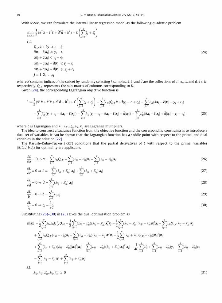
Example 1. Consider a data set listed in Table 1 taken from Tanaka and Lee [37]. The interval linear regression model isassumed to be YðxÞ ¼ A0 þ A1x. With the proposed method, we obtain the possibility Y�ðxÞ and the necessity Y�ðxÞ model asin (33)–(34). The results are illustrated in Fig. 1.

Y�ðxÞ ¼ ð7:4390;12:0320Þ þ ð8:5740;2:6940Þx ð33ÞY�ðxÞ ¼ ð7:4390;0:4250Þ þ ð8:5740; 0:5980Þx ð34Þ

The possibility Y�ðxÞ and the necessity Y�ðxÞmodels by Tanaka and Lee [37] and Hong and Hwang [14] are listed in (35)–(36)and (37)–(38), respectively.

Y�ðxÞ ¼ ð7:3110;11:8560Þ þ ð8:3710;2:4620Þx ð35ÞY�ðxÞ ¼ ð7:3110;0:1680Þ þ ð8:3710; 0:5140Þx ð36ÞY�ðxÞ ¼ ð7:5536;11:3333Þ þ ð8:4345;2:6786Þx ð37ÞY�ðxÞ ¼ ð7:5536;0:4107Þ þ ð8:4345; 0:5774Þx ð38Þ

Table 2 presents the proposed method with a linear kernel along with the results computed by Tanaka and Lee [37] andHong and Hwang [14]. The comparison is shown by using the measure of fitness [37], which defines how closely the possi-bility output for the jth input approximates the necessity output for the jth input. We can find that the interval coefficientsfrom all methods are similar.

uY ðxjÞ ¼1q

Xq

j¼1

c0 þPn

i¼1cijxijjc0 þ

Pni¼1cijxijj þ d0 þ

Pni¼1dijxijj

ð39Þ

where q is a sample size and 0 6 uY 6 1.

t of Example 1.

1 2 3 4 5 6 7 8

1 2 3 4 5 6 7 8[15,30] [20,37.5] [15,35] [25,60] [25,55] [40,65] [55,95] [70,100]

0

10

20

30

40

50

60

70

80

90

100

110

1 2 3 4 5 6 7 8

Input x

Inte

rval

Out

putY

Observation

Possibility Model

Necessity Model

CenteraLine

Fig. 1. Interval linear regression model with RSVM.

Table 2Comparison results of the measure of fitness of Example 1.

No. Tanaka and Lee [37] Hong and Hwang [14] Proposed method

1 0.0476 0.0705 0.06952 0.0713 0.0938 0.09313 0.0889 0.1106 0.11034 0.1025 0.1234 0.12355 0.1133 0.1334 0.13396 0.1221 0.1414 0.14237 0.1295 0.1480 0.14938 0.1356 0.1535 0.1551uY 0.1013 0.1218 0.1221

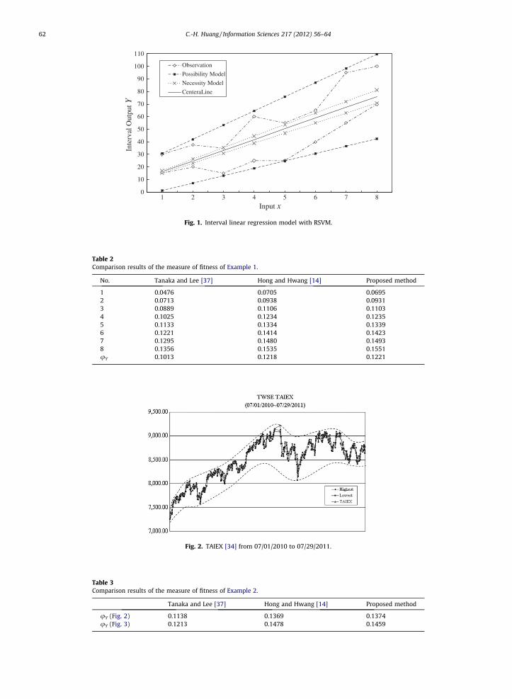
Fig. 2. TAIEX [34] from 07/01/2010 to 07/29/2011.

Table 3Comparison results of the measure of fitness of Example 2.

Tanaka and Lee [37] Hong and Hwang [14] Proposed method

uY (Fig. 2) 0.1138 0.1369 0.1374uY (Fig. 3) 0.1213 0.1478 0.1459

62 C.-H. Huang / Information Sciences 217 (2012) 56–64

Fig. 3. TAIEX [34] from 07/01/2009 to 07/29/2011.

C.-H. Huang / Information Sciences 217 (2012) 56–64 63

Example 2. To illustrate the proposed method dealing with large-scale data sets, we use the Taiwan Stock Exchange Capi-talization Weighted Stock Index (TAIEX) [34] from 07=01=2010 to 07=29=2011 and 07=01=2009 to 07=29=2011. For this dataset, we use a Gaussian kernel [12,27] where r ¼ 2:0 and the regularization constant C ¼ 500. The results are illustrated inFig. 2 and Fig. 3. Table 3 presents the proposed method with a Gaussian kernel along with the results computed by Tanakaand Lee [37] and Hong and Hwang [14]. The comparison is shown by using the measure of fitness [37].

5. Conclusions

This report proposes a reduced support vector machine approach in evaluating interval regression models. The main ideaof the proposed method is to reduce the number of support vectors by randomly selecting a subset of samples. Here, we esti-mate the interval regression model with non-fuzzy inputs and interval output.

In future studies, both interval inputs–interval output and fuzzy inputs–fuzzy output will be considered. Additionally, in aconventional SVM, the sign function is used as the decision-making function. The separation threshold of the sign function is0, which results in an excursion of separation margin for unbalanced data sets. The aim of the hard-margin separation mar-gin is to find a hyperplane with the largest distance to the nearest training data. However, the limitations of the hard-marginformulation are as follows:

1. There is no separating hyperplane for certain training data.2. Complete separation with zero training error will lead to suboptimal prediction error.

Therefore, the soft-margin method will be considered to modify the excursion of separation margin and to be effective inthe ‘‘gray’’ zone. The idea of the soft-margin method is to maximize the margin and minimize the training error.

Acknowledgment

The author would like to appreciate the editor in chief and five anonymous referees for their useful comments and sug-gestions which helped to improve the quality and presentation of this manuscript. The original version of this article waspresented in the International DSI Conference 2007 & APDSI Conference 2007, Thailand. Also special thanks to the NationalScience Council, Taiwan, for financially supporting this research under Grant No. NSC 98-2410-H-424-004-.

References

[1] M. Arun Kumar, R. Khemchandani, M. Gopal, S. Chandra, Knowledge based Least Squares Twin support vector machines, Information Sciences 180(2010) 4606–4618.

[2] A. Bisserier, R. Boukezzoula, S. Galichet, A revisited approach to linear fuzzy regression using trapezoidal fuzzy intervals, Information Sciences 180(2010) 3653–3673.

[3] J.J. Buckley, T. Feuring, Linear and non-linear fuzzy regression: evolutionary algorithm solutions, Fuzzy Sets and Systems 112 (3) (2000) 381–394.[4] C.J.C. Burges, A tutorial on support vector machines for pattern recognition, Data Mining and Knowledge Discovery 2 (1998) 121–167.[5] A. Celmin�š, A practical approach to nonlinear fuzzy regression, SIAM Journal on Scientific and Statistical Computing 12 (1991) 521–546.[6] Y.H.O. Chang, B.M. Ayyubb, Fuzzy regression methods: a comparative assessment, Fuzzy Sets and Systems 119 (2001) 187–203.[7] V. Cherkassky, F. Mulier, Learning from Data–Concepts Theory and Methods, John Wiley and Sons Inc., New York, 1998.[8] C. Cortes, V.N. Vapnik, Support vector networks, Machine Learning 20 (1995) 273–297.[9] P. D’Urso, R. Massari, A. Santoro, A class of fuzzy clusterwise regression models, Information Sciences 180 (2010) 4737–4762.

[10] P. D’Urso, R. Massari, A. Santoro, Robust fuzzy regression analysis, Information Sciences 181 (2011) 4154–4174.[11] H. Drucker, C.J.C. Burges, L. Kaufman, A. Smola, V.N. Vapnik, Support vector regression machines, in: M. Mozer, M. Jordan, T. Petsche (Eds.), Advances in

Neural Information Processing Systems, MIT Press, Cambridge, Massachusetts, 1997, pp. 155–161.

64 C.-H. Huang / Information Sciences 217 (2012) 56–64

[12] S. Gunn, Support Vector Machines for Classification and Regression, ISIS Technical Report University of Southampton, 1998.[13] D.H. Hong, C.H. Hwang, Support vector fuzzy regression machines, Fuzzy Sets and Systems 138 (2003) 271–281.[14] D.H. Hong, C.H. Hwang, Interval regression analysis using quadratic loss support vector machine, IEEE Transactions on Fuzzy Systems 13 (2005) 229–

237.[15] H. Ishibuchi, H. Tanaka, Fuzzy regression analysis using neural networks, Fuzzy Sets and Systems 50 (1992) 257–265.[16] J.T. Jeng, C.C. Chuang, S.F. Su, Support vector interval regression networks for interval regression analysis, Fuzzy Sets and Systems 138 (2003) 283–300.[17] J. Kacprzyk, M. Fedrizzi, Fuzzy Regression Analysis, Physica-Verlag, Heidelberg, 1992.[18] Y.J. Lee, S.Y. Huang, Reduced support vector machines: a statistical theory, IEEE Transactions on Neural Networks 18 (1) (2007) 1–13.[19] Y.J. Lee, O.L. Mangasarian, RSVM: reduced support vector machines, in: Proceedings of 1st SIAM International Conference on Data Mining, 2001.[20] K.-M. Lin, C.-J. Lin, A study on reduced support vector machines, IEEE Transactions on Neural Networks 14 (2003) 1449–1559.[21] S. Maldonado, R. Weber, J. Basak, Simultaneous feature selection and classification using kernel–penalized support vector machines, Information

Sciences 181 (2011) 115–128.[22] O.L. Mangasarian, Nonlinear Programming, McGraw-Hill, New York, 1969 (Society for Industrial and, Applied Mathematics, 1994).[23] O.L. Mangasarian, Mathematical programming in data mining, Data Mining and Knowledge Discovery 42 (1) (1997) 183–201.[24] O.L. Mangasarian, Generalized support vector machines, in: A.J. Smola, P.L. Bartlett, B. Schölkopf, D. Schuurmans (Eds.), Advances in Large Margin

Classifiers, MIT Press, Cambridge, Massachusetts, 2000, pp. 135–146.[25] O.L. Mangasarian, D.R. Musicant, Massive support vector regression, in: M.C. Ferris, O.L. Mangasarian, J.S. Pang (Eds.), Complementarity:

Applications,Algorithms and Extensions, Springer, 2001.[26] O.L. Mangasarian, D.R. Musicant, Data discrimination via nonlinear generalized support vector machines, in: M.C. Ferris, O.L. Mangasarian, J.S. Pang

(Eds.), Complementarity: Applications, Algorithms and Extensions, Springer, 2001.[27] C.A. Micchelli, Interpolation of scattered data: distance matrices and conditionally positive definite functions, Constructive Approximation 2 (1986)

11–22.[28] R. Savitha, S. Suresh, N. Sundararajan, Fast learning Circular Complex-valued Extreme Learning Machine (CC-ELM) for real-valued classification

problems, Information Sciences 187 (2012) 277–290.[29] B. Schölkopf, Support Vector Learning, R. Oldenbourg Verlag, Münich, Doktorarbeit, TU Berlin, 1997.[30] B. Schölkopf, C.J.C. Burges, A.J. Smola, Advances in Kernel Methods: Support Vector Learning, Massachusetts, MIT Press, Cambridge, 1999.[31] B. Schölkopf, A.J. Smola, Learning with Kernels: Support Vector Machines, Regularization, Optimization, and Beyond, MIT Press, Cambridge,

Massachusetts, 2002.[32] B. Schölkopf, A.J. Smola, K.-R. Müller, Nonlinear component analysis as a kernel eigenvalue problem, Neural Computation 10 (1998) 1299–1319.[33] A.J. Smola, B. Schölkopf, A tutorial on support vector regression, Statistics and Computing 14 (2004) 199–222.[34] Taiwan Stock Exchange Capitalization Weighted Stock Index (TAIEX). <http://www.twse.com.tw/en>[35] H. Tanaka, Fuzzy data analysis by possibilistic linear models, Fuzzy Sets and Systems 28 (1987) 363–375.[36] H. Tanaka, I. Hayashi, J. Watada, Possibilistic linear regression analysis for fuzzy data, European Journal of Operational Research 40 (1989) 389–396.[37] H. Tanaka, H. Lee, Interval regression analysis by quadratic programming approach, IEEE Transactions on Fuzzy Systems 6 (1998) 473–481.[38] H. Tanaka, S. Uejima, K. Asai, Fuzzy linear regression model, IEEE Transactions on Systems Man and Cybernetics 10 (1980) 2933–2938.[39] H. Tanaka, S. Uejima, K. Asai, Linear regression analysis with fuzzy model, IEEE Transactions on Systems Man and Cybernetics 12 (1982) 903–907.[40] A. Unler, A. Murat, R.B. Chinnam, mr2PSO: a maximum relevance minimum redundancy feature selection method based on swarm intelligence for

support vector machine classification, Information Sciences 181 (2011) 4625–4641.[41] V.N. Vapnik, The Nature of Statistical Learning Theory, Springer-Verlag, New York, 1995.[42] V.N. Vapnik, Statistical Learning Theory, John Wiley and Sons Inc., New York, 1998.