a real-time digital spectrum analyzer - nasaa real-time digital spectrum analyzer r. b. mccullough...
TRANSCRIPT

A Real-Time Digital
Spectrum Analyzer
by
R. B. McCullough
GPO PRICE $
CFSTI PRICE(S) $
Hard copy (HC)
Microfiche (MF),
ff 653 July 65
November 1967
"1_1_ _. 1 q 80-_I _ (A_'WES._ON NUMBER)@ ) (THRU)
(T_ASA CR-OR TMX OR AD NUMBER}
Scientific Report No. 23
Prepared under
National Aeronautics and Space Administration
Research Grant No. NsG-377
RflDIOS(IEn(E LDBOROTORY
§TgnFORD ELE(TROnI(S LgBORgTORIE|sTgnFORO UlUVERSlT9 • STilnFORD, (IILIFORfllII
https://ntrs.nasa.gov/search.jsp?R=19680004335 2020-05-30T23:45:23+00:00Z

SEL-67-099
A REAL-TIME DIGITAL SPECTRUM ANALYZER
by
R. B. McCullough
November 1967
Scientific Report No. 23
Prepared under
National Aeronautics and Space Administration
Research Grant No. NsG-377
Radioscience LaboratoryStanford Electronics Laboratories
Stanford University Stanford, California

A Real-Time Digital Spectrum AnalyzerR. B. McCullough
Sci. Rept. 23NsG 377December 1967
PRECEDING PAGE BLANK NOT FILMED.ABSTRACT
In the past, spectral analysis has been done almost
exclusively by analog equipment. The main stumbling block
for digital spectral analysis has been the enormous number of
computations necessary to calculate the spectrum digitally.
This research develops a new algorithm for digital spec-
tral analysis in real time. This new algorithm is intended
for implementation by special-purpose circuitry using cur-
rently available integrated circuits. Maximum sampling rates
above I MHz can be realized in continuous real-time operation.
This is much faster than any other existing algorithm can
operate.
A closed-form analytical expression is developed for the
passband characteristics of the discrete Fourier transform
operation. This expression is used to evaluate in detail the
effectiveness of several time-domain and frequency-domain
operations aimed at improving the passband characteristics.
A hardware design is presented which makes use of certain
novel features of this newreal-time algorithm. Among these
features is the use of shift registers in which only the in-
puts and outputs are available. This permits use of very
long integrated circuit shift registers in very small packages
since very few inputs and outputs are required. This feature
would not be an advantage in realizing this algorithm in a
general-purpose computer, but it definitely is in special-
purpose hardware.
iii SEL-67-099
PRECEDING PAGE BLANK NOT FILMED.

III.
VI.
CONTENTS
Page
I. INTRODUCTION .................. i
II. SPECTRUM ANALYSIS ............... 3
A. Definition of Spectra ........... 3
B. Analog Spectrum Analysis ........ 4
C. Digital Spectrum Analysis ......... 6
D. Comparison of Analog and Digital Analyzers . 8
DISCRETE FOURIER TRANSFORMS .......... I0
A. Discrete Fourier Transform Equations .... i0
B. Efficient Operation Grouping ........ ii
C. Rules for Constructing _low Charts ..... 17
D. Computational Savings ........... 19
E. Power Spectra ............... 19
IV. PASSBAND CHARACTERISTICS ............ 21
A. Infinite Number of Samples ......... 21
B. Finite Number of Samples .......... 23
C. Multiplicative Constants .......... 28
V. IMPROVING PASSBAND CHARACTERISTICS ....... 30
A. Time-Domain Operations .......... 30
B. Easily Implemented Operations ....... 31
C. Frequency-Domain Operations ........ 35
D. Equivalent Time-Domain Operation ...... 43
E. Double Hanning .............. 47
HARDWARE IMPLEMENTATION OF FOURIER TRANSFORMALGORITHM .................. 52
SEL-67-099 iv

VII.
Vlll.
IX.
XQ
XI.
A. Basic Functional Building Block ......
B. Basic Functional Block Using 0nly OneMultiplier .................
C. Hardware Adders ..............
D. Hardware Multipliers ............
E. Simplification of Multipliers .......
SPEED OF OPERATION ...............
A. Calculation Time ..............
B. Pipelining .................
REAL-TIME ALGORITHM ..............
A. Real-Time Operation ............
B. Derivation of Real-Time Algorithm .....
C. Hardware Requirements ...........
SINGLE AND MULTIPLE CHANNEL FILTERS ......
A. Realization ................
B. Applications ................
DIGITAL SPECTRUM ANALYZER OUTPUT ........
A. Complex Sinusoidal Output .........
B. Updating Frequency Estimates ........
C. Frequency Components of Envelope ......
TIME-SHARED REAL-TIME ALGORITHM ........
A. Derivation of Algorithm ..........
B. Hardware Reduction .............
C. Output Schemes ...............
55
57
57
59
61
61
63
66
66
66
68
73
73
75
78
78
82
83
86
86
89
9O
v SEL-67-099

Pa_
D. Multiplying Constants ........... 93
E. Outputs in Normal Order .......... 93
F. Passband Shaping .............. 97
G. Example Using Estimate Updating ...... 99
H. Algorithm Modification To Permit Hannlng . . 105
XII. SUMMARY AND SUGGESTIONS .......... 113
A. Summary .................. 113
B. Suggestions for Further Research ...... 114
APPENDIX A. CONVOLUTION THEOREM ........... 116
APPENDIX B. INTERPOLATION .............. 119
BIBLIOGRAPHY ..................... 125
TABLE
Number
, Number of samples vs calculation time and
maximum sample rate for 12-bit sample words
(0.025 percent accuracy) ............62
SEL-67-099 vi

ILLUSTRATIONS
F i_Fe Page
i. Analog filter bank analyzer .......... 5
2. Swept-frequency analyzer ............ 5
3. Digital spectrum analyzer using linear
difference equations .............. 7
4. Real-time digital spectrum analyzer ...... $
5. Flow chart of calculations for n = 24 ..... 16
6. Derivation of spectrum of sampled f(t) .... 22
7. Derivation of spectrum of finite impulse train 24
$. Convolution of F(_) with spectrum of sampling
impulse train ................. 27
9. Typical h(t) envelope obtained by shifting
bits of digitized data input .......... 33
I0. Magnitude of H(_) for an easily mechanizedh(t) ...................... 35
Ii. Addition of three adjacent weighted spectralestimates ...................
12. Passband for
13. Passband for
14. Passband for
15.
16.
17.
18.
19.
K _- --0• 426 ............
K = -0.5 .............
Time-domain window equivalent to weighted
summation of adjacent frequency-spectru_estimates ...................
Equivalent time- and frequency-domain
operation ...................
Flow graph for hanning operation ........
Passband achieved by hanning twice .......
Flow chart of basic computational block ....
38
39
4O
41
46
47
48
51
_4
vii SEL-67-099

Figure
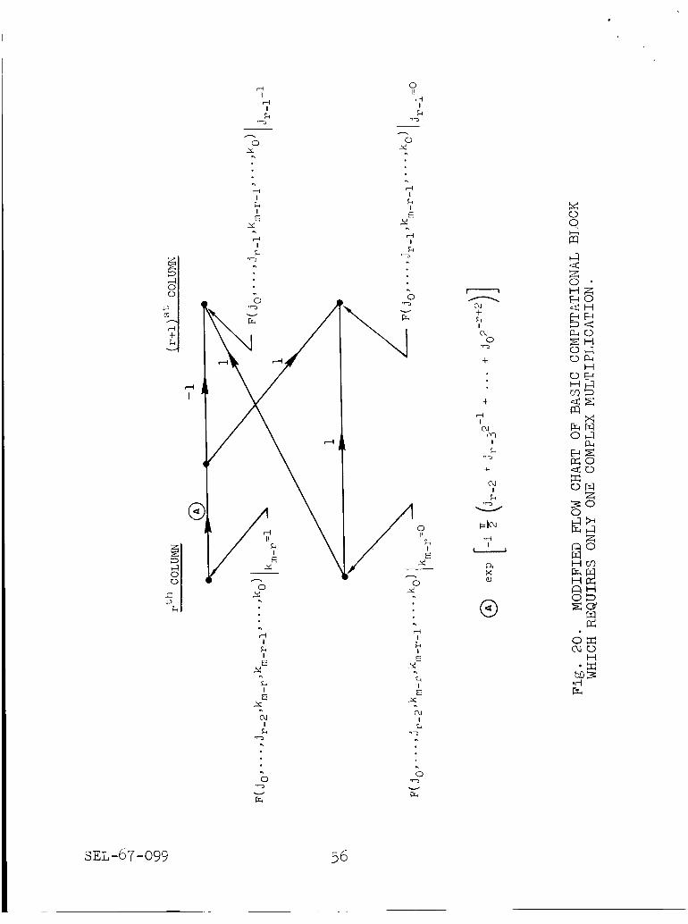
20. Modified flow chart of basic computational
block which requires only one complexmultiplication ................. 56
21. A 12-bit straight binary adder ........ 57
22. A 12-bit straight binary multiplier ...... 58
23. Calculation circuitry utilizing pipelining . . 64
24. Modified algorithm for real-time operation . . 67
25. Real-time algorithm using only one multiplier
per basic function block ............ 69
A
26. Derivation of single-channel filter for FI0from real-time algorithm ............ 74
27. Digital lowpass filter derivation ....... 75
28. F8 passband filter derivation ......... 76
29. Shifting of f(t) past transform circuitry . . 78
A
30. Derivation of F(_0, t = (n-l)T + kT) ..... 79
31. Time sequence of outputs and sample sets they
depend on ................... 87
32. Time-shared real-time algorithm (outputs in
jumbled order) ............... 88
33. Timing circuitry ................ 91
34. Oscilloscope output .............. 92
35. Wired storage for multiplying constants .... 94
36. Flow chart for frequency outputs in normalorder .................... 95
37. Phase variations of frequency spectrumestimates ................... 97
38. Cosine of frequency (_3 + _4)/2 in thefrequency domain ................ i00
SEL-67-099 viii

Figure
39.
40.
41.
Example of relative phase errors in hanned
estimates using updating ............
Computation flow graph to be used with hanning
(outputs in jumbled order) ...........
Computation flow graph to be used with hanning
(outputs in normal order) ...........
42.
43. Magnitude "passband characteristic" of inter-
polated output ..............
Rotation of frequency estimate output ....
Pag__e
lO4
106
107
120
124
ix SEL-67-099

ACKNOWLEDGMENT
The guidance and encouragement of Dr. Allen Peterson
and Dr. Bruce Lusignan during the progress of this research
are gratefully acknowledged.
SEL-67-099 x

Chapter I
INTRODUCTION
Spectrum analysis has historically been performed almost
exclusively by analog equipment. Digital equipment has not
been used because of the tremendous number of computations
that must be performed in order to calculate the spectrum.
In 1965 Cooley and Tukey derived a new algorithm which
reduced the number of computations necessary by the factor
of (log 2 n)/n for calculating n spectrum points from n
input samples. This algorithm and its offspring have made
practicable the computation of spectra on large general-
purpose computers. These applications have generally been
either non-real time or real time with very low frequency
components.
A new algorithm is derived here which is suitable for
real-time operation at sample rates exceeding i MHz. This
algorithm is intended for implementation by special-purpose
hardware using integrated circuits. It also features
continuous rather than "batch" processing.
Considerable attention is paid to the passband charac-
teristics of these algorithms. A convenient closed-form
analytic expression is derived for the passband of the basic
Fourier transform algorithm. This expression is used to
evaluate in detail the effectiveness of several time-domain
and frequency-domain operations aimed at improving the pass-
band characteristics.
i SEL-67-099

A hardware design is presented which uses currently
available integrated circuits. The maximum sampling rate
obtainable is determined to be above i MHz. The author feels
that the algorithm and design presented offer the best
solution for rapid real-time spectral analysis.
SEL-67-099 2

Chapter II
SPECTRUMANALYSIS
A. Definition of Spectra
Spectrum as used here will refer to either the voltage
spectrum, the energy spectrum, or the power spectrum of the
input signal. The vo!tage spectrum is the Fourier transform
of the input signal as given by
oo
F(co) = _ f(t) e -i°°t dt (2.1)--00
The voltage spectrum will in general be complex.
The energy spectrum is obtained simply by taking the
magnitude squared of the voltage spectrum:
--IF(®)12= f(t) e -id°t
2
dt (2.2)
The energy spectrum is purely real.
A problem arises in the use of the energy spectrum since
real signals of unbounded time duration possess energy
spectra which are unbounded. In general, the energy per unit
time, i.e., the power, will be bounded. The power spe.ctrum
can be defined as
I _-i -i_tP(_) = lim _-_ f(t) e
2
dt (2.3)
The power spectrum P(_) is also purely real and in addition
is bounded for most input signals.
3 SEL-67-099

An alternate way of arriving at the power spectrum is
to take the autocorrelation function of the input and then
Fourier transform it:
P(_) : S_. tT-_lim9-_i_T- f(T) f(t + T) d-i_t
e dt (2.4)
It is apparent that no matter which spectrum is desired
or what path is followed to obtain it, some form of Fourier
transform will be involved.
B. Analog Spectrum Analysis
Spectrum analysis has traditionally been done with
analog equipment. Two basic systems have been used: filter
banks and swept analyzers. The most straightforward approach
is shown in Fig. I. In this system a bank of n tuned band-
pass filters is used. Each filter passes components of the
input signal that lie within a narrow band of frequencies
between _j - A_/2 and _j + A_/2, where _j is the center
frequency of the filter and A_ is its bandwidth. The out-
put of each filter is then squared and averaged to give an
estimate of the signal power at the frequency _j. The
circuitry is repeated n times to give n power spectrum
estimates.
The second approach is illustrated in Fig. 2. In this
system the input signal is mixed with the output of a swept-
frequency oscillator to produce the sum and difference fre-
quencies. The difference frequency is then passed through a
SEL-67-099 4

f(t) r
n
BANDPASSF_LTERS
•
•
0
k
g .,=...==._
SQUARINGCIRCUITS
l A
P(w 0 )
m
m
m
,==----.O_
POWERSPECTRUMESTIMATE
AVERAGINGCIRCUITS
Fig. i. ANALOG FILTER BANK ANALYZER.
f(t)
I MIXER ]_t
SWEPT-FREQUENCYOSCILLATOR
Fig.
BAND PASS
FILTER J I
wf
SQUARING HCIRCUITAV E RAGER
2. SWEPT-FREQUENCY ANALYZER.
A
p (wf+w s )
5 SEL-67-099

bandpass filter, squared, and averaged to produce an estimate
of the power spectrum at a frequency _s + _f' where _s is
the oscillator frequency and _f is the filter frequency.
As the oscillator frequency is varied, the frequency at
which the power spectrum is estimated varies. This analyzer
requires considerably less hardware than the filter-bank
analyzer.
C. Digital Spectrum Analysis
Digital spectrum analysis may be performed in a number
of ways. In all cases, the analog input signal is sampled
and converted into a series of digital numbers. Calculations
must then be performed on these numbers to produce another
series of numbers which represent the spectrum of the signal
being analyzed. The problem lies in being clever enough in
the organization of the calculations that they may be per-
formed in a minimal amount of time by a minimal amount of
hardware.
Weaver, Mantey, Lawrence, and Cole at Stanford University
[1966] have used a set of linear difference equations to
obtain an estimate of the spectrum of the input. The ana-
lyzer they implemented is shown in Fig. 3. Each of the
difference equations is of the form:
y(nT) = aox(nT) + alx[(n-l)T] + ..- + akx[(n-k)T]
-blY[(n-l)T ] - b2Y[(n-2)T] - ... - bmY[(n-m)T]
(2.5)
SEL-67-099 6

FAST SLOW
_SAMPLER ,_SAMPLER
,,,l.Jo._[,FILTER[/| G!
Y2 (nLT)
2)
_n 2Ya (nLT)
:k-j
------o
-------o
GL(Z ) ( )2 n_k_ j Y
Fig. 3. DIGITAL SPECTRUM ANALYZER USING LINEAR DIFFERENCE
EQUAT IONS.
Since the previous outputs are included as inputs to the
analyzer, long time spans of data can be included in rela-
tively few calculations to yield good resolution in the
frequency domain. Unfortunately the inclusion of previous
outputs also introduces the possibility of instability into
the difference equations. This analyzer is a direct digital
equivalent of the analog filter-bank analyzer.
Other digital spectrum analyzers have been built by
digitally computing a Fourier transform of the input samples.
By and large these analyzers have been realized on general-
purpose digital computers and have been operated in non-real
time. The transform algorithms used have been some form of
7 SEL-67-099

the Cooley-Tukey algorithm or a derivation thereof. These
algorithms "batch-process" the data; that is, computation is
not begun until a batch of n samples is collected. The
processing produces n outputs and then halts until the
next set of n inputs is collected. The batch-process
nature of these algorithms makes them unsuited for continuous
real-time operation.
The present effort also utilizes a digital Fourier trans-
form. However, a new algorithm is derived which permits
efficient real-time operation. The block diagram of the
proposed analyzer is shown in Fig. 4. The analog input
signal f(t) is sampled and converted into a digital number;
these numbers are used in the computation of the Fourier
transform of the input. Finally, the magnitude of the trans-
form is squared to obtain the power spectrum of the input.
The particular algorithm used is especially well suited to
realization by special-purpose hardware built from integrated
circuits.
f(t) J A/D I fs(t)
I CONVERTERI TRANSFORM ICOMPUTATIONI
CIRCUITRY J
F(w)
Flg. 4. REAL-TIME DIGITAL SPECTRUM ANALYZER.
D. Comparison of Analo_ and Di$ital Analyzers
The analog analyzer has historically held the edge in
practical implementation because it has required far less
SEL-67-099 8

hardware than the digital spectru_ analyzer. The analog
analyzers have suffered from problems characteristic of any
analog instrument. In particular, it is difficult to keep
the gain and frequency bands of a large number of analog
filters from drifting with time, temperature, and other
environmental changes. On the other hand, the characteris-
tics of the digital analyzer are completely insensitive to
its environment.
The major stumbling block to the implementation of
digital spectrum analyzers has been the large number of
computations necessary to perform the digital Fourier trans-
form. This problem has been alleviated greatly by the
Cooley-Tukey algorithm which is derived in detail in
Chapter III. Furthermore, the advent of integrated circuits
has made the building of large, special-purpose computational
units a practicable approach. The digital spectrum analyzer
proposed in this research will become even more attractive
as integrated circuit technology progresses.
9 SEL-67-099

Chapter III
DISCRETE FOURIER TRANSFORMS
A. Discrete Fourier Transform EQuations
The basic operation in any spectrum analysis is the
taking of the Fourier transform. In our digital spectr_n
analyzer we will be working with samples of the input taken
every T seconds. The transform we compute will in fact
be the transform of the sampled input rather than the true
input.
The sampling can be represented mathematically as multi-
plication of the input f(t) by an impulse train of period
T •The resultant fs(t) is given by
oo
fs(t): f(t) - k<) (3.1)
The Fourier transform of the sampled signal is given by
FS(a_) = _ f(t) _ _(t -kT)e -i_t dtm_
k_
Carrying out the integral yields
(3.2)
Fs(_) = ! f(kT) e -ic°kT (3.3)
Equation (3.3) is the basic equation for the digital
computation of spectra. It involves taking the samples of
the input f(kT), multiplying by a complex number e-i_kT
SEL-67-099 i0

and summing over all the available samples. These operations
must be performed for every desired value of _. Conse-
quently, if we want n points of the spectrum and we have2
n time samples to work from, we will have to perform n
complex multiplications and additions.
B. Efficient 0peration Grouping
If the operations are grouped appropriately we can make
some savings in the number of operations performed. Let us
look at the problem of calculating n samples of Fs(_ )
evenly spaced between _ = 0 and _ = [(n-l)2_]/nT from
the n input samples of fs(t) from t = 0 to t = (n-l)T.
Equation (3.3) may be written
n-i
Fs(C° = n2_T_) = ! f(kT)exp(-i -_J2_ kT)
k=0
(3.4)
where the equation is to be evaluated for all values of j
from j = 0 to j = n-l.
Let us write the indices j and k as binary numbers
• m-2J = Jm-i 2m-I + Jm-2 2 + "'" + Jl 2 + J0 (3.5)
k = km_l 2m-I + km_2 2m-2 + ... + k12 + k0 (3.6)
By writing j and k as above we have made the tacit
assumption that the number of samples is less than or equal
to 2m. Let us now shorten our notation in the following
manner:ii SEL-67-099

nT, : Fs(Jm-l'Jm-2'''''Jl'J0 ) : Fs(J)
f(t = kT) = f(km_l,km_2,...,kl,k0 ) = f(k)
With this shortened notation, Eq. (3.4) can be written
n-i
__ 2m-I
k=O
+ "'" + J0)
• (km_12m-i + ... + k0) ]
(3.8)
(B.9)
The product in the exponential contains powers of 2
between 20 and 22m-2. Let us write this product out in
more detail:
m-i
22m-2 22m-3Jm-lkm-i + I J2m-3-rkr +
r=m-2
+ 2m+l
m-i m-i
2mJm+l-rkr +
r=2 r=l
Jm_rkr
m-I
+ 2m-I
r=0
Jm-l_rkr
m-2
+ 2m-2
r=0
Jm_2_rkr + ...
2 i
+ 22 _ J2_rkr + 2 _
r=0 r=0
Jl_rkr + Joko (3.1o)
SEL-67-099 12

Notice that this product is in the form of powers of 2 with
integer coefficients.
The maximum number of samples we have provided for is
2 m. Let us then take full advantage of our capability by
setting the number of samples n = 2m. Doing this, and
using (3.10), we can expand the exponential of (3,9) as
follows :
exp(-i 2_ jk) exp[-i 2_ (Jm_12m-i +-_- : -_- ... + jo)(km_12m-I + .. + ko) ]
m-I
: exp(-i2_2m-2jm_ikm_l)exp(-127r2 m-3 _ J2m-3-rkr )''"
r=m-2
m-i m-i
• exp(-i2_2 _ Jm+l_rkr ) exp(-i2_ _ Jm_rkr )
r=2 r=l
m-I 2
• exp(-i2_2 -I _ Jm-l-rkr ) ... exp(-i2_22-m _ J2-rkr )
r=O r=O
I
" exp( -i2Tr21-m _. Jl-rkr)exp(-i2_2-mjoko) (3.11)
r=O
The first m-I exponentials in (3.11) are of the form
exp(-i2_p), where p is an integer, and hence are identi-
cally equal bo one. Equation (3.11) may consequently be
greatly simplified to:
13 SEL-67-099

m-i m-2
exp(-i _ Jk) exp(-12_2 -I _ Jm_l_rkr)exp(-±_2-2 _ Jm_2_rkr)_ . ° o
r=O r=O
2 i
• exp(_i2_22-m _ J2-rkr) exp(-12_2 l-m _ Jl-rkr)
r=O r=O
• exp (-i2_2-mJoko) (3.12)
In Eq. (3.12), km_ I appears only in the first exponential;
km_ 2 only in the first two; km_ 3 only in the first three;
etc. Regrouping the exponentials, we have
exp (-i -_--2_Jk) = exp (-i2_km_lJo 2-I) exp [-i2_km_2(Jl 2-I + j02-2)]
• exp[-121rkm_3(J22-1 + J12-2 + J02-3)]
• exp[-12Wkl(Jm_p2-1 + ... + JO2-m+l)]
• exp[-i27rk O(jm_12-1 + ... + JO2-m)] (313)
The expression for the exponential in (3.13) may be put
back into the summation in (3.9) and the summation over k
may be broken into many sums over the individual kr. The
result is
f(k) exp(-i2_km_lJ02-1)}
•
SEL-67-099
I14

•oxp[i_kl(jm22I
•o_p[i2_ko(Jm121+..÷_o2m)] (3.14)
Each of the variables k being summed upon in Eq. (3.14)r
has only the value 0 or i, since each is a coefficient of a
power of 2 in the binary number representation of k.
Equation (3.14) may be evaluated by beginning at the
innermos% sum and working outward. Let us arrange the 2m
samples of f(k) in a column in order of ascending values
of the binary number k. These samples are shown in the
left-hand column of Fig. 5 for m = 4, or 16 samples.
Figure 5 is a flow graph for the transform computations.
The innermost sum of (3.14) is over km_ I = O, i and
can be written out as
I
km_l=O
f(k) exp(-i2_km_lJo 2-I)
= f(O,km_2,...,ko) e0 + l,km_2,...,k0) expi_[-i2_J02-1}f(
(3._5)
Thus the inner sum is seen to be a function of the km_2,
km_3,...,k 0 and J0" There will be 2m of these functions
which we will label F(J0,km_2,...,k0). These are shown in
the second column of Fig. 5 arranged in order of ascending
15 SEL-67-099

IIII
III0
II01
II00
I011 fll
I010
1001 f9
I000 f8
0111 fz
0110 f6
0101 f5
0100 f4
0011 f3
0010 f2
0001
0000
i
• 2_Fig. 5 FLOW CHART OF CALCULATIONS FOR n = .
SEL-67-099 16

value of the binary numbers jo 2m-I + km_22m-2 + ... + k020"
The nodes represent the value of the f_ctions and are
arrived at by summing the value of all incoming arrows
multiplied by the value of their respective origins.
The next innermost sum of (3.14) can be expanded as
i
• . ._m2
k m_2 =0
: F(Jo,O,km_3,...,k 0) e0 + F(Jo,l,km_3,...,k0)
•exp -i2_(J12-i + J02-2)] (3.16)
The set of equations (3.16) gives the transition between
column 2 and column 3 of Fig. 5.
C. Rules for Constructing Flow Charts
The continued expansion of Eq. (3.14) will result in a
completed figure of the form of Fig. 5. The following
general rules may be deduced for a generalized figure using
2m time samples to obtain 2m frequency samples:
•
.
A figure for 2m
2m points each.
The points of the first column will be the original
time samples arranged in order of the magnitude of
km_l 2m-1 + km_22m-2 + ... +their arguments:
k12 + k O.
samples will have m+l columns of
17 SEL-67-099

3. The points of the second column will be points of an
array
of the
F(Jo,km_2,...,kl,ko). In general, the pointsth
r column will be points of an array
F(Jo,Jl,...,jr_2,km_r,km_r_l,...,kl,ko), arranged
in order of the magnitude of the number jo 2m-I
Jl 2m-2 Jr-2 2m-r+l 2m-r + k+ + ... + + km_ r m-r-1
+ ... + k12 + kO.
thAll arrows leaving points in the r column for
thwhich the r index is zero will have weight i and
will go horizontally to points in the (r+l) st
column whose indices are the same, and to points
2m-r-i
thwhose indices are different in the r index only.
th5. All arrows leaving points in the r column for
•
thwhich the r index is i will have weight
[exp -i2_(Jr_l 2-I + jr_22 -2 + . . + jl 2-r+l + jo 2
and will go horizontally to points in the (r+l) st
column whose indices are the same, and to points
thwhose indices are different in the r index only.
Note that the values of the weights are determined
by Jo through Jr-i which are the first r
indices of the destinations of the arrows•
The points in the (m+l) st column will be the points
of the spectrum Fs(Jo,Jl,...,Jm_l)
order of the magnitude of the number
arranged in
jo 2m-I + Jl 2m-2
+ "'" + Jm-22 + Jm-l" Note that the indices Jo
through Jm-i are reversed from their normal order.
SEL-67-099 18

D. Computatignal Savings
It can now be seen that by arranging the computations in
the order described, considerable labor may be saved. In
particular, rule i tells us that we have m2 m points to cal-
culate to obtain the spectrum as opposed to the n 2 = (2m) 2
operations required to calculate the spectrum by direct
application of Eq. (3.4). This computational algorithm was
originally derived by Cooley and Tukey.
In Chapter VIII a new algorithm is derived which is even
better suited to hardware implementation. Although the
number of operations is not reduced, the manner in which
they are performed in real time permits considerable savings
in hardware.
E. Power S_ectra
Up to this point we have been calculating the Fourier
transform of the input waveform. In order to get the power
spectrum of the input, we must take the square of the
magnitude of the voltage transform already calculated. It
is the power spectra rather than the voltage spectra that is
the expected output from a "spectrum analyzer."
The power spectra may be arrived at in two ways. One is
to form the autocorrelation function of the input and take
the transform of the autocorrelation. The other way is to
transform the input to get the voltage spectrum, and then
take the magnitude squared of the voltage spectra to get the
19 SEL-67-099

power spectrum. We will choose the latter route as it will
require far less in the way of additional circuitry.
The output of the real-time Fourier transform algorithm
is a set of n complex numbers. Each of these numbers is
of the form A + iB. The magnitude squared then will be
given by A2 + B2. The squaring can be accomplished by
putting A or B in both the x and y inputs of a multi-
plier such as the one designed in Chapter VI. Getting the
magnitude squared will then require two multipliers and one
adder for each of the n output samples.
SEL-67-099 20

Chapter IV
PASSBANDCHARACTERISTICS
A. Infinite Number of Samples
The result of performing a discrete Fourier transform
yields the transform of the sampled input signal rather than
the transform of the original input.
Figure 6 shows the derivation of the sampled signal's
spectrum in terms of the spectrum of the unsampled signal.
Here it is assumed that the sampling is done by an infinite
string of impulses spaced T seconds apart. The transform
of this string of impulses is another string of impulses in
the frequency domain of area I/(2_T) spaced 2_/T radians
apart. The sampling impulses and their transform are shown
in Fig. 6b. Multiplying by the first string of impulses in
the time domain is equivalent to convolution of the original
frequency spectrum with the infinite string of impulses in
the frequency domain as shown in Fig. 6c. Equations (4.1a)
through (4.1c) describe the operations illustrated in Fig. 6.
The convolution theorem is derived in Appendix A.
f(t ) --4-
oo oo
i 2_ )
(4.la)
(4.ib)
2i SEL-67-099

TIME DOMAIN
f(t}
=-tv
FREQUENCY DOMAIN
F(_)
a. f(t) and its transform F(_)
T. 8(t-k_-) __L :E 8(_-k _-_)-o0 2w'_" -OD
=-t
b. Sampling impulses and their transform
fs(t)= f(kz') T. 8(t-kz')-oO
Fs(=)=_.L._ _o4.'T
c. Sampled fs(t) and its transform
Fig. 6. DERIVATION OF SPECTRUM OF SAMPLED f(t).
SEL-67-099 22

fs(t)=oo
f(t) _ 5(t-_OO
Fs( )
Fs(*) = 2Tr _ 57 -
_00 _00
oo
1 F(mOO
As illustrated in Fig. 6c and Eq. (4.1c), Fs(_), the
spectrum of the sampled signal, is the sum of an infinite
number of the original F(_) with their centers spaced 2_/T
apart along the frequency axis. If the spacing 2_/T is
great enough, there will be no overlap of the individual
spectra and the sampling has thus introduced no errors.
B. Finite Number of Samples
Up to now we have been talking about using an infinite
number of samples in the time domain so that the convolution
in the frequency domain is with an infinite string of impulses.
Any finite machine we build must, of course, make calculations
based on only a finite number of time samples. We now
naturally ask what errors are introduced because we don't use
an infinite number of samples.
Figure 7 illustrates the derivation of our finite string
of impulses by which we will multiply our time function f(t)
to get a finite number of samples f(t). F(_) will then be
a convolution of F(_) with the transform of the sampling
function as shown in Fig. 7c.
23 SEL-67-099

TIME DOMAIN
SQUARE ENVELOPE
T= n'r = J
....-,_ I_.... t
n"E"
FREQUENCY DOMAIN
T exp (-i oj ---_)
v
ujT2
a. Square envelope and its transform
T_8 (t-k',") Z',r_--(_D
b. Sampling impulses and their transform
n-I
T. _ (t-kT)k=O
=--t
• T 2_"s,n_"(_-k _ )co
z -o[-,[ c,_-,,_)] ,,_4.n-Z "r -o0 T_(=- )
c. Finite sampling impulse train and its transform
Fig. 7. DERIVATION OF SPECTRUM OF FINITE IMPULSE TRAIN.
SEL-67-099 24

To get a finite number of impulses we take the square
window of Fig. 7a and multiply it by the infinite s_ring of
impulses in Fig. 7b. Note that the window is of width nT
and extends from -c to nT - _ (c being arbitrarily
small) and thus will contain exactly n impulses.
The transform of the square window is
exp[-i_(}- c)]T sin (coT/.2)_T/2
where for
exp (-i_ }). When we multiply the window and the string of
impulses in the time domain we must convolve
with a string of impulses in the frequency domain.
(%.2b)
The
result is that the transform of our finite sampling function
as shown in Fig. 7c is
n-i
_(t - kT) _---_
k:O g_2T
exp[-i T (do - k _)] T T (co - k 2_) (4.2c)k=-_ 2
_- @ - k = i, a plot of the magnitude
of the transform of our sampling function will look as shown
in Fig. 7c. The spacing between the (sin x)/x functions is
25 SEL-67-099

2_/v. Remembering that T = nT, we find their height is
n/4_ 2 and their width varies inversely with n, the number
of samples used.
When a time function f(t) is sampled by multiplying byn-i
E 6(t - kT), then the spectrum of the sampled ftu_cbioi_k=O
f(t) can be expressed as the convolution of the original
spectrum F(_) with the spectrum of the sampling impulses
as given by (4.2c). Thus
^ IF(_o) =
O0
/FI oo-mOO
oo si=(nT )I exp -i -_- co nT
k=-_ -_--co - nkTr
J_ (_.3)
A
It is actually F(_O) which we are calculating by our
discrete Fourier transform. From (4.3), F(COo) is seen to
be a weighted average of the true values of F(co) in the
vicinity of _0'
Let us assume that the sampling rate is high enough so
that F(_) is essentially zero for -_/T _ _ _ _/T. This
is the Nyquist rate. Then the limits on the integration in
(4.3 may be changed as follows:
/ ecomesJ-_ _=_O-_/T
(4._)
SEL-07-099 26

A
Since we are interested in F(_0) only for
-_/T _< e0 -< T/T, the spectrum F(@ 0 -_) as shown in the
convolution in Fig. 8 will overlap with only the (sin x)/x
function centered at @ = O. Hence the summation in (%.3)
will consist only of one term. Consequently we can write
oo
n
: /sin nT
denT-- (13
2 (%.5
In summary, it has been shown that the output of a digital
spectrum analyzer computed using a finite number of samples
2.___T
I
-Tr
TRA.SFO_.O.SA.PL,.O_U.CT.O.--
NSFORM OF
vv-_,-- : Q,I
2"n"T
Fig. 8. CONVOLUTION OF F(co)
IMPULSE TRAIN.
WITH SPECTRUM OF SAMPLING
27 SEL-67-099

A
will be an estimate F(_O) of the true value of F(_O). The
n_mber F(co0) obtained has been shown to be a weighted
average of the true values of F(_) in the vicinity of _0"
The weighting function or "passband characteristic" is a
(sin x)/x function whose width varies inversely with i-i,
the number of samples used.
C. Multiplicative Constants
In Eq. (4.5), F(_O) is a somewhat biased estimate of
F(_). Let's assume F(_) is roughly constant and equal to
F(_O) in the vicinity of _0; then Eq. (4.5) may be
simplified to
sin nT
nF(c°o)8_3 / exp(-i _ co) nT-_-coF( O) -- (4.6)
Carrying through the integration we find
., F(o_ 0 )(4.7)
Hence the calculated value of F(_O) differs from the
true value by a multiplicative constant of i/(8_2_). This
multiplicative constant need not pose any problem depending
on what use is made of the calculated spectrum. For instance,
the digital spectrum may be reconverted to analog for an
oscilloscope display of amplitude vs frequency. In this case
the gain of the vertical amplifier of the oscilloscope may be
adjusted to compensate for the multiplicative constant.
SEL-67-099 28

However, if a digital printout or other digital display
is desired, the multiplicative constant will prove harder to
deal with. The best solution in this case would probably be
to use an amplifier with gain 8_2T in front of the sampling
process.
29 SEL-67-099

Chapter V
IMPROVING PASSBANDCHARACTERISTICS
A. Time-Domain Operations
In Eq. (_.5), the output of our digital spectrum analyzer
for _0 was expressed as a weighted average of the true
values of F(_) in the vicinity of _0" The weighting func-
tion is to our digital spectrum analyzer what the passband
characteristics are to an analog spectrum analyzer. As
expressed in Eq. (4.5) the passband of our digital spectr_
analyzer has the shape
nT
8_ exp -in _ (_.i)nT
Note that this is precisely I/(8_3T) times the transform of
the square envelope which we used to multiply the infinite
sampling impulse train in order to obtain a finite number of
sampling impulses.
This observation leads us to ask if we cannot modify the
passband characteristics of our digital spectrum analyzer by
changing the multiplying envelope. The answer is that indeed
we can. In particular, if we use an envelope h(t) which is
nT seconds wide, the output of our analyzer for co0 will be
F(_0)_ = _l f F(_o -_) H(_) d_ (5.2)
SEL-67-099 30

where H(_) is the Fourier transform of h(t).
We would like H(_) to be infinitesimally narrow, i.e.,
an impulse. The only way this can be achieved is to make
h(t) infinitely wide. This, of course, is an impossibility
for it means we would need an infinitely large machine to
handle our infinite number of samples. The problem is analo-
gous to the problem of shaping the far-field pattern of an
antenna array by changing position and size of the array
elements.
Our primary purpose in modifying the envelope h(t) will
be to improve our resolution in the frequency domain [i.e.,
to make H(_) narrower]. Our secondary purpose will be to
eliminate spurious responses which occur when two adjacent
frequency components in the incoming signal are superimposed
by the integral of (5.2) and either reinforce or cancel each
other.
B. Easil_ Implemented Operations
Since we are doing our calculations digitally, certain
h(t) envelopes will be easier to achieve than others. In
antennas, for instance, the elements of an array might be
cosinusoidally weighted. Such a weighting would be difficult
to realize digitally. Other arrays might be density weighted,
which means that certain elements of the array are not driven
or used. This would be easy to realize digitally since it
merely means dropping some of the samples and replacing them
by zero in the calculation. Also, any h(t) in which the
31 SEL-67-099
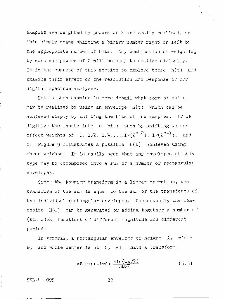
samples are weighted by powers of 2 are easily realized, as
this simply means shifting a binary number right or left by
the appropriate number of bits. Any combination of weighting
by zero and powers of 2 will be easy to realize digitally.
It is the purpose of this section to explore these h(t) and
examine their effect on the resolution and response of our
digital spectrum analyzer.
Let us then examine in more detail what sort of gains
may be realized by using an envelope h(t) which can be
achieved simply by shifting the bits of the samples. If we
digitize the inputs into p bits, then by shifting we can
effect weights of i, 1/2, I/4,...,I/(2P-2), I/(2P-I), and
0. Figure 9 illustrates a possible h(t) achieved using
these weights. It is easily seen that any envelopes of this
type may be decomposed into a sum of a number of rectangular
envelopes.
Since the Fourier transform is a linear operation, the
transform of the sum is equal to the sum of the transforms of
the individual rectangular envelopes. Consequently the com-
posite H(_) can be generated by adding together a number of
(sin x)/x functions of different magnitude and different
period.
In general, a rectangular envelope of height A, width
B, and whose center is at C, will have a transform:
AB exp(-i_C) sin(_oB/2) B'/z
(5.3)
SEL-67-099 32

h(t) -
J
e_D
-_-i-
i
....i--i......
IL i L l ,
........ 2
--_I14
-_---] 1/16
NT
t _
Fig. 9. TYPICAL h(t) ENVELOPE OBTAINED BY SHIFTING BITSOF DIGITIZED DATA INPUT.
A sum of such rectangular envelopes will have a transform:
sin (_oBj/2 )
_AjBj exp(-imCj) _Bj//2 ' ' (5.g)J
Let us confine our attention to envelopes which are symmetri-
cal about their centers, then the phase factor in (5.4) will
be the same for all j and may be brought outside the
summation.
33 SEL-67-099

sin (_Bj/2)exp(-i_C) I AjBj ' [oBj/2 (5.5)
J
.thThe factor A.B. is simply the area under the OJJ
We should note that Aj = i/2 J andrectangular envelope.
Bj. _<Bj+I. Referring to Fig. 9 it is easy to see that each
coefficient AkBk is smaller than or equal to the sum of all
the AjBj for j _ k + i. This observation puts limits on
the relative sizes of the various functions we are going to
sum together.
Let us attempt to get a better feeling for the process
that is occurring by working out the passband characteristics
for the envelope shown in Fig. 9. Evaluating (5.5) we obtain
16 T) {T sin 16 _Texp( -i_\ IS _T
15 sin 15 _T+ i--_T 15 _T
+ 7 T sin 14 _T + _ T sin 13 _T'I_ o_m '13 cot
6T sin 12 _T + lit sin ii _T_ (5 6)+i2 _T 11 _T / "
The passband characteristics expressed in Eq. (5.6) are
plotted in Fig. i0 and can be compared to the passband
characteristics of the original rectangular h(t) which are
plotted in the same figure. The result is a passband which
is generally wider and lower than the original. Similar
SEL-67-099 34

25
\\\\
\
--I H(_u) I FOR SQUARE h(f) WINDOW WITH SAME NUMBER OF SAMPLESAS h(t) SHOWN IN FIG. 9
\
H(_)T
15
\\\\\
I FOR h(t) WINDOW OF FIG. 9
Fig. i0. MAGNITUDE OF H(_) FOR AN EASILY MECHANIZED h(t).
results are obtained for other simply implemented h(t) which
require only a shifting of the bits of the input samples.
C. Frequency-Domain Operations
Some operations which prove difficult to implement in the
time domain may be much more simply performed in the frequency
domain. Suppose, for instance, that we simply add to each
frequency estimate the value of the two adjacent estimates
multiplied by a constant K. The estimate at _0 can be
written as
35 SEL-67-099

n
--00
TIT - CO)sin -_- (COO ,, -dec
(w0 -CO)
(5.7)
The adjacent estimates are centered at
be written as
_o +-(2Tr/n_) and can
co
+- _ f _(_)--co
exp[-i _ (C°O + nT
sin -_- _0 +- n-_ - dec
nT ( 27r co)-T _o +n-Y -
(5.s)
Using the identity
e -iv = - i
we may express (5.8) as
o [ ]_F _o -+_ - 8_-"7_ F(_) e_p -i _ (_0
sin y C°O + n-%" - dec
, ii )nT (c°0 -- nm"Y- + 27r __
(5.LO)
Combining (5.7) and (5.10) yields
SEL -67 -099 36

oo
sin-9( o+nT ] dco (5 ii)
- K nT 2_
_- (COO + nT---- co)
,%
F(%)The spectral estimate as given in (5.11) is seen
F(m) of the input weighted
by a passband characteristic which is the sum of three shifted
(sin x)/x type functions. Figure ii illustrates the three
(sin x)/x functions. For ease of illustration the complex
exponential (whose magnitude is one) has not been shown. The
value of K can be adjusted so that the two adjacent
(sin x)/x functions will partially cancel the sidelobes on
the central (sin x)/x function. Perini [196g] studied a
mathematically similar problem in the shaping of the far-field
patterns of linear antenna arrays.
Figures 12 through 14 show the combined passband charac-
teristic for several interesting values of K. Figure 12 is
for K = 0, which gives the original (sin x)/x passband.
Figure 13 is for K = -0.g26, which yields a zero at the peak
of the first sidelobe of the original passband. This choice
to be equal to the true spectra
37 SEL-67-099

/
sin '-_" (_o-_)
n'r, +2w" .sin 2 I_o -n-_-(_)
_ - K_-----_.---
Fig. ii. ADDITION OF THREE ADJACENT WEIGHTED SPECTRAL
ESTIMATES •
of K makes the close-ln sidelobes very small.
Figure 14 shows the passband for K = -0.5. This partic-
ular choice of K gives sidelobes which fall off as
i/(co0 _ _)3 rather than i/co0 - co. To show this we must
expand Eq. (5.11) using sin (x _ _) = - sin x:
n
._CO
(coo-nT
7
i + K )K + coo - co 2v2rr _ co coO + _ - coCOO - n-_ nT
dco (5.12)
SEL-67 -099 38

Fig. 12. PASSBAND FOR K = 0.
39 SEL-67-099

Fig. 13. PASSBAND FOR K = -0.426.
SEL-67-099 40

Fig. 14. PASSBANDFOR K = -0.5.
41 SEL-67-099

Putting (5.12) over a common denominator gives
oo
n/ )]_(co 0) = _ F(co) exp -i -_--(coO - co
[ {2_2 ]•,(2K + 1)(%- _)2 _ _, I
•L( o_ _ _ (% - _)J
sin _ (_0 - _)
nT
-T
dco (5.1.3)
If we now set K = -1/2 we obtain
oo
n / F(a)) exp[-i _ (co0- co)] sin nT - co)_- (coo
(})_(_o-_)s
27_
For co near coO' the (coO - co)3
can be written
2 nT _ CO)- _ 7- (coo
term is small and (5.14)
n
_(co0) _ _ / F(co)exp[-i _ (coO-co)]--00
nT - Co)sin -_- (coo
nT
"T" (coo- cO)dco
for I(})_(coo co)3J<<1"2(% - co)l
z_and K = - kD.zP)2
For _ far from coO,
(5.14) can be written
the _0 - cO term is negligible and
SEL-67-099 42

co
--00
for
2
nT
sin -T -do3
1and K = - 7 (R.76_
Equation (5.16) explicitly points up the i/(_ 0 _ _)3 aprons
of the passband characteristic for K-- -1/2. Q.E.D.
The addition of F(_0) to K times the two adjacent
frequency estimates is an easily implemented modification and
has been shown above to result in substantially reduced side-
lobes in the passband. The special case of K : -1/2 is
especially easy to implement as no multiplication is needed.
The factor of 1/2 is achieved by hardwiring a shift of i bit.
This special case has been dubbed "harming" by Blackman and
Tukey [1959].
D. Equiyalent Time-Domain Operation
The summing in the frequency domain could be replaced by
an equivalent time-domain operation. As it turns out, such
an operation is far more complicated to implement from a
hardware standpoint. To find out what the equivalent time-
domain operation is, we first note that the summing of the
three (sin x)/x functions can be expressed as a convolution
of a single (sin x)/x function with three impulses. Expanding
the terms in brackets in (5.11) yields
43 SEL-67-099

- K_in_ (_o2_ _) sin_ (_o-_)
nT +
nT 2_ co -_ (0_0-T °_0 - n--F-
- K2"ff - d,,))
nT 2_ _)-T (C_O + h"F -
/ [sin _ (_0 - _ - _),.] d__- [__(_-_)+_(_)__(_+_1]t _ (_o-_ _)-oo
(5.x7)
Plugging (5.17) back into (5.11) gives
co
:_ _ [-_M(_o _)]f
[_ _ .]2_] in -_-(co0 - _ - _)/
+ 4(_) - KSk_ + n'_/] nTd_ dec
_(_o -_- n)(5.18)
By reversing the order of integration and pulling out a
factor of exp(-i _ _) we obtain
(5.19)
Referring to (5.7), the inner integral of (5.19) is seen to
be (8_3)/n F(_O - _ )"
Consequently we find
SEL-67-099 44

oo
o) :_00
exp (-i nT (5.2o)
Equation (5.20) is in the form of a convolution in the fre-
quency domain which is equivalent to a multiplication in the
time domain by an h(t) window function whose transform is
given by
h(t) _---_2_{6(m) - K[5(co - _-.) +_2_ (co +
The window h(t)
exp _-inT -2-
(5.21)
then can be determined to be
2Tr (t nT)h(t) : I - 2K cos n-_ - -2-
: i + 2K cos 2 --it (5.22)nT
Figure 15 shows the effect of this window function on the
input data samples for a K value of -0.426.
Realization of this increase in resolution by multiplying
the n input samples by the appropriate h(t) will require
n complex multiplications. Realization of the increase by
working in the frequency domain will require n complex
multipliers and 2n complex adders as shown in Fig. 16. How-
ever, if K is set at -1/2, then the multiplications can be
replaced by hardwired shifting and complementing and we are
left simply with 2n adders. Consequently, working in the
45 SEL-67-099

2_'th(t) _---I - 2K cos
/ \
_t
SAMPLING t = n I"IMPULSES
Fig. 15. TIME-DOMAIN WINDOW EQUIVALENT TOWEIGHTED SUMMATION OF ADJACENT FREQUENCY-
SPECTRUM ESTIMATES.
frequency domain here is really only attractive if the value
of K can be set to -1/2 or some other easily realized con-
stant multiplier.
A new real-time, hardware-oriented algorithm is derived
in Chapter VIII. In using this algorithm the input is never
in a stationary array, and hence premultiplication by an
appropriate h(t) window is further complicated. It is for
this reason and for the reasons in the above paragraph that
we will choose to do our modifications in the frequency
domain at the output of the computation circuitry. We will
also choose a value of K = -1/2 for ease of implementation
as mentioned above.
shown in Fig. 17.
SEL-67-099
The resulting windowing circuitry is
_6

n-W
J
l.-.J
n
DATA _ }
WORDS "'rr(3_
JE
TRANSFORM
" COMPUTATION
CIRCUITRY
n
FREQUENCYSPECTRUM
ESTIMATES
a. Premultiplication by h(t) window
n
DATA
WORDS
TRANSFORMCOMPUTATION
CIRCUITRY
z
<i:EzDO
or_.,_ n-2
,., t _FREQUENCY_o SPECTRUM_'_ ESTIMATES
_0
,-.,,,jrrIJ.
b. Equivalent frequency-domain convolution
Fig. 16. EQUIVALENT TIME- AND FREQUENCY-DOMAIN OPERATION.
E. Double Hanning
A second hanning has been used by some researchers in
order to improve the resolution further. Let us call the
double-hanned signal F(_0)._ We can then write
47 SEL-67-099

A
F15
-112
FI4 FI4-I
F 13 FI3
^F 12 FI2
A A
F II FII
^F I0 FI 0
^F 9 F9
^F8 F8
^F 7 F7
^F 6 F6
AA A
F 5 F5
AA ^
F 4 F4
AA A
F 3 F3
^ _F 2 ; F2
F I FI
A
F0
Fig. 17. FLOW GRAPH FOR HANNING
OPERATION.
SEL-67-099

A
F(_ol 2 nT -_$(_0+_) (5.23
Using Eq. (5.11) for F(_0) yields
F(c°0) : - [ - 2" nT
{ ^ ^( _) _( _)}i i F(_o) + _0 + fly - ZF _0 +- (5.24)-7 -7 n<
Collecting like terms
_(_o):_ _(_o _ nT
-_(_o+_) +_(_o+_) (5.25
A
We may further express F(_O) in terms of the true _(_),
yielding
s(ooo) = _ s(_) exp[-i _ (_0 - co)] [_n T 4_
+sin_ (_o 2_-co -_) 3
nT 2"n" 2(_0-_ - _-t_i__ (_o-_)
(_o - _o)
+nT( _)sin -_ co0 - a) +
nT 2_-_-(co0 - co+ _-)
i+_ J
@_ (5.26)
_9 SEL-67-099

From (5.26) we see that the double-banned spectral estimate
_(_0) has a passband characteristic which is the sum of
five shifted (sin x)/x-type functions. Since it was not
immediately obvious that this passband was going to be an
improvement over the single-harmed case, a computer program
was written to compute and plot this passband. The results
of this plot can be seen in Fig. 18.
Although the sidelobes do drop off more rapidly than the
single-harmed passband, the central peak has been made con-
siderably broader. The improvement in passband character-
istics in going from single hanning (Fig. 14) to double
banning (Fig. 18) is much less marked than is the improvement
in going from no banning (Fig. 12) to single hanning. Since
the windowing circuitry must be approximately doubled to
implement double hanning, it is felt that the single-hanned
frequency estimate is the best compromise.
SEL-67-099 50

Fig. 18. PASSBANDACHIEVED BY HANNING TWICE.
51 SEL-67-099

Chapter VI
HARDWAREIMPLEMENTATIONOF FOURIER TRANSFORMALGORITHM
A. Basic Functional Building Block
Let us now investigate the problems of mechanizing the
Cooley-Tukey algorithm. For n = 2m input samples the flow
chart of the calculations will contain m+l columns repre-
senting m stages of calculation plus the original sample
points. Each of the points in the (r+l) st column will be
ththe complex sum of one of the numbers in the r column
thand another of the numbers in the r column multiplied by
a complex constant.
Generally speaking, all the numbers dealt with will have
a real part and an imaginary part. Hence all additions will,
in fact, be two additions (Real + Real; Imaginary + Imaginary)
and all multiplications will be four multiplications (Re × Re;
Re × Im; Im x Re; Im X Im).
thLet us group together in the r column pairs of points
which differ only in the r th index. If we do this, we note
that each such pair of points affects only the corresponding
pair of points in the (r+l) st column. Furthermore, the
pair of points in the (r+l) st column depends on no other
thpoints in the r column but this pair. This is a very
important observation because it allows us to isolate a small
functional block which is repeated throughout the calculation
circuitry.
SEL-67-099 52

This observation also sets a lower limit on the number
of operations that must be performed in parallel; that is,
we must calculate the points in pairs. After each pair of
the (r+l) st column is calculated, the corresponding pointsth
of the r column may be discarded and calculation of
another pair started. Hence, we must, as a minimum, provide
storage for n+2 complex numbers.
Figure 19 illustrates the flow chart of this basic func-
tional block described in the previous paragraph. We may
split the basic operation in half so that we will be calcu-
lating, for every point, the sum of one previous point and
one point multiplied by a constant according to Eq. (6.1).
F(Jo,...,Jr_l,km_r_l,...,ko )
= F(Jo,...,Jr_2,km_r,km_r_l,...,kO)]km_r= 0
F(Jo'''''Jr-2'km-r'km-r-l'''''ko) km-r=l+
r)](6.1)
The value of the exponential constant is dependent only
on where we are in the overall calculation flow chart. The
fact that it is a constant will make the multiplying circuitry
simpler.
Since the multiplying constant has a magnitude of less
than one, as we move from one column to the next, the
53 SEL-67-099

4O0_
HII
!
O
I
IE
H!
°r_
HI
I
IE
C_I
°ca
OII
I
--a
O
I
IE
r_I
•r--a
I
I
i
OJI
•r-3
IGJ
O
+
+
(Y3I
I
+
_JIGJ
I
+
I_J
bOJ
N©
®
IOJ
0
+
+
cqIOJ
_qI
+
oJIOJ
OJI
"_"3
@J.M
Ii i
®
0
0
_4
Z0H
E_
or._)
r..)
H
r_
o
0
o
r-.-t
.r-I
•r- 0
b
SEL-67-099 5_

magnitude of the numbers will increase by less than a factor
of 2. Hence, as we move to the right each column will in
general require one more bit in its representation than did
the previous column. Consequently, if we begin with 2m
each q-bit samples, the spectrum calculated will contain 2m
words of q+m bits each.
B. Basic Functional Block Using 0nly One Multipliero
The relationship between the two multiplicative constants
needed can be seen in the basic functional block of Fig. 19.
Note specifically that the constant on the top path can be
written
exp[-i2_( 2-I + Jr_22
m 2 -3+ _a.ir__2 + ... +
= exp[i2 Ijr22-2+ +j02r)]
The right-hand side of (6.2) is seen to be just the nega-
tive of the multiplicative constant on the downward-sloping
path. Hence Fig. 19 can be modified so that only one complex
multiplication is needed rather than the two required by
straightforward application of the flow graph. Figure 20
shows the modified basic functional block.
This modification reduces the total number of complex
multiplications for the complete flow chart from m2 m to
m2 m-I Since the majority of the computation time and
55 SEL-67-099
E
4o
I
II
I
O
,-4I
I
!
!
I
E
I
C_I
0_
v
OI!
I
O
I
IE
!
,-4!
I
I
O4I
0_
v
X_r_0
0H_BO
O_oP-4
H
r_
X_MO_
C_
_0
m
_00
_0
Hr._
_HO_
O_04C)
H
b.O:_._t
SEL -67 -099 56

circuitry is spent in multiplication, this simple modification
allows a savings of about one-half of the circuitry necessary.
C. Hardware Adders
The operations of addition and multiplication must be
implemented. A parallel binary adder of the appropriate
number of bits can be quite easily implemented using currently
available integrated circuits. Figure 21 illustrates a 12-bit
adder constructed from 4-bit adder integrated circuits which
are available commercially from Texas Instruments.
Bll B9 All A9
I.,o1.!,IN
CARRY 211 _10 Z9 28
B7 B 5 A7 A 5 B 5 B I A3 A I
1"1"1 '1I l"l'°l i-,,,, I [ II
27 2e 25 24 23 2a 21 2o
Fig. 21. A 12-BIT STRAIGHT BINARY ADDER. All integratedcircuits are Texas Instruments 4-bit adder modules.
D. Hardware Multipliers
Multiplication of two binary numbers can be accomplished
by a shifting and adding procedure. When one of the numbers
is known ahead of time (as are the exponential constants),
the hardware may be greatly simplified. The simplification,
57 SEL-67-099

however, makes one multiplier different from another and
hence increases the number of types of circuits needed.
Figure 22 shows one possible implementation of a 12-bit
straight binary multiplier. This is a completely general
I:_ ! _ ! ! !_ ! TI!i _:_
I _,,_,, _ _,e. A.e,, A..., ,_,S. A.e,, A.B,, A.B. _e. A,e, Aoeolr'tCARRY 12-BIT STRAIGHT BINARY ADDER _1 I %
Yo xz
_..__... _
..__-., _
._.._....__
e X3
,D X s
e X?
e X I
el X I
- XlO
* )tit
Fig. 22. A 12-BIT STRAIGHT BINARY MULTIPLIER.
SEL-67-099 58

circuit since each of the multiplicands x and y can be
any binary number. The building of a multiplier in this
fashion has in general not been economically feasible in the
past, and actually probably is not yet. However, as inte-
grated circuit technology progresses, this multiplier becomes
more and more attractive. For instance, at the present time
Texas Instruments is producing commercially a _-bit parallel
adder in a single integrated circuit chip. At the present
state of the art, then, the multiplier of Fig. 22 would
require something on the order of 72 integrated circuit chips
to implement with commercially available products. This number
could probably be cut in half through design of special-purpose
chips. It is not inconceivable that this complete circuit may
some day be implemented in a single chip.
E. Simplification of Multipliers
When the value of one of the multiplicands is known ahead
of time, the multiplier of Fig. 22 may be greatly simplified.
Knowing the values of x 0 through Xll will allow us to
eliminate all the AND gates and, on the average, half the
adders from Fig. 22. To prove this, note that if any x i
is I then we may eliminate the associated row of AND gates
and simply tie the Yi directly into the associated adder.
Further, if any x i is 0 we may eliminate both the
associated AND gates and the associated adder since the sum
of the adder is simply equal to the other input. The x i
59 SEL-67-099

will on the average be half l's and half O's; hence on the
average we may eliminate half the adders.
Thus the necessary multipliers could be made using an
average of about 15-1/2 of the existing 4-bit adder chips
currently available from Texas Instruments. This is a
considerable savings over the previously mentioned 72 chips
per multiplier.
Since the numbers dealt with will be complex, every point
of the calculation will require four multiplications and two
additions. If there are 2m sample points, there will be
4m2m multiplications and 2m2m additions. If 12-bit numbers
are used as proposed, the results of the multiplications will
be 24-bit numbers which must be rounded off again to 12 bits
before we add. This will usually involve merely dropping the
12 least significant bits. The multipliers can be simplified
still further if these bits are not calculated at all, since
they will be dropped anyway.
SEL-67-099 6O

Chapter VII
SPEEDOF OPERATION
A. Calculation Time
The time required to perform the calculations will set
an upper limit on the sample rate and thus set an upper limit
on frequency response of our spectrum analyzer. It will be
instructive to work out an example to see what can be done
with currently available products. The Texas Instruments
4-bit adder has a carry propagation delay of 30 ns for 4 bits
or 90 ns for 12 bits. This is the longest path for the 12-bit
adder. The longest path for the multiplier is through the
90 ns of carry delay and down the average of 5-1/2 rows of
adders at about 50 ns each, then through another 90 ns of
carry delay for a total of 445 ns. Add to this the 90 ns of
the addition and we get about 545 ns for each column of the
calculation.
Using this value it is possible to derive Table i, which
relates the number of 12-bit samples used to the approximate
maximum sampling rate and consequently the highest frequency
estimate of the resulting digital spectrum analyzer. Note
that the calculation time varies with the number of columns
or the log of the number of samples. The calculation time
also increases roughly directly proportional to the number of
bits in the samples.
61 SEL-67-099

Table i
NUMBEROF SAMPLESVS CALCULATION TIME AND MAXIMUMSAMPLERATE FOR 12-BIT SAMPLEWORDS(0.025 PERCENTACCURACY)
mNumber of
Samples (2 m)
i 2
2 4
3 8
4 16
5 32
6 64
7 128
8 256
9 512
i0 1,024
ll 2,048
12 4,096
13 8,192
14 16,384
CalculationTime
0.545
1 .O9
i .635
2.18
2.73
3.27
3.81
4.36
4.91
5.45
6.00
6.54
7 .O8
7.63
Max imum
SampleRate
(kHz)
1840
918
612
458
367
306
262
229
204
184
167
153
141
131
Max imum
FrequencyEstimate
(kHz)
920
459
3O6
229
183
153
131
115
lO2
92
84
77
71
66
Referring to Table i, it should be noted that the maximum
sample rates are somewhat faster than the conversion rates of
currently available 12-bit A_D (analog to digital) converters
whose conversion times will be in the range of 20 to i00 _s.
This need not be a problem (except possibly a financial one)
since it should be an easy matter to use several "Sample and
Hold" amplifiers followed by several A/D converters, and then
use a digital multiplexer to present the digitized samples to
the calculator in the correct time sequence.
SEL-67-099 62

The described implementation of a digital spectrum
analyzer is several orders of magnitude faster than other
schemes realized on digital computers (e.g., Weaver et al
[1966]; Cooley & Tukey [1965]; Larson & Singleton [1967];
Gentleman & Sande [1966]). It is this extra speed that
should make possible a practical real-time digital spectrum
analyzer. Whether or not the extra cost of a specially
constructed parallel arithmetic unit is "practical" will
depend on the particular application.
B. Pipelining
Some increases in speed may be made through use of a
technique known as "pipelining." In this technique, a second
set of samples is input into the calculator before the results
of the first set of data have come out the output end. In
this way the data sets will proceed in waves from input to
output in the calculator.
In general, the number of waves is limited by the differ-
ences in time delays along different paths in the calculation.
That is, the results will be meaningful only so long as one
wave does not overtake the wave in front of it or lag into
the wave behind it. Otherwise the results will become
scrambled and meaningless.
If all paths in the calculation required exactly the same
time, the calculation could be pipelined up to any desired
speed. Unfortunately it is a practical impossibility to make
all the paths the same time length. If, however, a stage of
63 SEL-67-099

memory is inserted between each column of the calculation,
we can gain in speed by a factor of m for 2m samples.
Figure 23 shows how this would be accomplished.
CLOCK
t-ic
INPUTSAMPLES
m
CALC
CKT
OUTPUTSAMPLES
Fig. 23. CALCULATION CIRCUITRY UTILIZING PIPELINING.
By clocking the storage registers and the input shift
register we can essentially make the delay along all paths
of the calculation constant. The delay will be equal to one
clock period times the number of columns in the calculation.
The clock period need only be long enough to allow for the
maximum time delay through a single column of the calculator.
This maximum delay would be about 820 ns for the multiplier
SEL-67-099 64

and adder described earlier. Thus the clock could be run at
a 1.2 MHz rate regardless of the number of input samples used.
This in turn means a sample rate and output rate of 1.2 MHz.
The maximum frequency estimate then would be raised to
600 kHz. And all this in real time!
The higher sampling rate, of course, means that even
more sample and hold circuits, more A/D converters, and more
inputs to the digital multiplexer would be needed. Thus,
while the potential for high-speed operation exists, it is
very expensive to realize.
65 SEL-67-099

Chapter VIII
REAL-TIME ALGORITHM
A. Real-Time Operation
When operating in real time we will run the input through
an analog-to-digital converter and store the results in a
shift register to be used as an input to the calculation
circuitry. As each new sample is brought in, all samples in
the register will be shifted down one position and the fre-
quency estimates will be recalculated.
When operating in this manner, the algorithm as described
in the previous chapters performs redundant calculations.
By modifying the algorithm to remove these redundancies in
real-time operation, it is possible to decrease the amount of
hardware necessary by approximately a factor of I/(log 2 n)
for n input samples.
B. Derivation of Real-Time Algorithm
Figure 24 illustrates the modified algorithm. The opera-
tions indicated in dashed lines between the first two columns
are among those that have been eliminated. Since the input
samples are being shifted one place each sample time, at any
time t the dashed operations would be calculating exactly
the same results that the solid operations calculated during
the previous sample time t - T. Consequently, rather than
repeat the calculation we may shift the results of the previ-
ous calculation into this register. Note that this is
SEL-67-099 66

r8 r12 r14 r15 ^I I II f15 • FI5
r8 I _7II10 f14 I
A
, \ FIII101 f13 D \ f I\ /
D \ / <4 II I O0 f12
\ I __ r io r 13 ^I011 fll SHIFT \\ / = = - = - FI3
REGISTER D ,,,
/\ D_ / _r 2 I F5I010 flO / "_ I/ I \ r9r9 ^
/ \ _ FSI001 f9 / \ r0
/ \ D_I,ooo '8 / \,/
I I r8 r 12 r14 ^011 I f7 / FI4
\ r6 ^OI I0 f6 _ ____ m F6I I
A
0101 I FIOD r2 ^
0100 rO F2I
0011 I r8 r12 F̂I2
r4 ,,,,q F40010 D, I
,8 ,,_
0 O01 F8
D rO ^0000 F o
Fig. 24. MODIFIED ALGORITHM FOR REAL-TIME OPERATION.
possible only because the constant multipliers were the same
for both the solid and the dashed operations. Further study
of the flow chart of Fig. 5 will indicate that the complete
second column of this figure may be generated by shifting
downward the results in row 7 and row 15.
Similarly the results in the third column may be gener-
ated by shifting downward the results in rows 3, 7, ii, and
15. Continuing in this fashion through all the columns, we
67 SEL-67-099

arrive at the much simplified algorithm shown in Fig. 24. By
using the single multiplier basic function block of Fig. 20,
the flow graph can be simplified further as shown in Fig. 25.
C. Hardware Requirements
Figure 25 requires one complex multiplier between
columns I and 2; two between columns 2 and 3; four between
columns 3 and 4; and so forth up to 2m-I between the last
two columns. The total number N of complex multipliers
needed is
N = i + 2 + 4 + 8 + ... + 2m-I (8.1)
This series can be brought into closed form as follows:
2N = 2 + 4 + 8 + ... + 2m-I + 2m
i + 2N - 2m = i + 2 + 4 + 8 + ... + 2m-I
(8.2)
= N (8.3)
Collecting terms yields N = 2m - i complex multipliers,
which amounts to a considerable savings in hardware over a
direct parallel implementation of the Cooley-Tukey algorithm
which would require N = m2 m complex multipliers.
The real-time algorithm of Fig. 25 can also be very easily
pipelined as mentioned in Chapter VII. In this case, then,
the shift registers would not represent an additional storage
register requirement but would merely be used in place of the
clocked registers shown in Fig. 23. The real-time algorithm,
SEL-67-099 68

in fact, uses fewer registers than the original. Figure 23
will require (m+l) columns of 2m registers each for
(m+l)2 m registers.
f15
f14rD
f15rD
f12D
fllD
floD
f9
f8
r 0 -I r 4 -IIp
I r 0f7 _'
r6 -I r7 -I ,A,FI5
I F7
D
I_ AF3FI5
I A
/%
F 9
F I
-I r4 -I r6 -I AFI4
I F6
I FIO
I F2
r0 -I r4-I ,,_
I FI20 ^
q
O' I F4
I F80
I F0
Fig. 25. REAL-TIME ALGORITHM USING ONLY ONE MULTIPLIERPER BASIC FUNCTION BLOCK.
The real-time algorithm will require 2m-I + I registers
in the first column; 2m-I + 2 registers in the secon6;
2m-I + 4
(m+l)st columns.
is given by
in the third; and so on up to
The total number R
2m in the mth and
of registers needed
69 SEL-67-099

R = (re+l) 2m-I + i + 2 + _ + ... + 2m-2 + 2m-I + 2m-I
= (re+l) 2m-I + 2m - I + 2m-I
i= 2m(_ m + 2) - i
which is less than the m2m needed for straightforward pipe-
lining of the Cooley-Tukey algorithm for all m _ _.
There is yet another great advantage of the real-time
algorithm that may not be immediately obvious. Specifically,
the advantage lies in the fact that only the first and last
stages of each shift register are looked at. This means that
cheaper types of shift registers may be used. For instance,
a simple delay line could be used as a shift register since
only the input and output are used. The delay line unfortu-
nately makes it virtually impossible to change sampling rates.
Although the delay line offers a large amount of storage
capacity at low cost, the problems of synchronizing its
operation with various sampling rates preclude its further
consideration.
In the area of clocked shift registers, there are several
choices. For example, a magnetic-core shift register can be
used since we don't have to look at all the intermediate
stages. The data in the first and last stages would be held
in flip-flop registers so that it would be available as inputs
to the multipliers and adders. The magnetic-core shift
SEL-67-099 70

register is more easily adapted to changing sample rates
than is the delay line.
Another possibility is the integrated circuit (IC) shift
register, such as Philco's 100-bit MOS shift register in a
single TO-5 can. Use of this device is possible only because
the real-time algorithm does not require access to the inter-
mediate stages along the shift register string.
It is important to note that if it were necessary to have
access to the intermediate stages, the size of the IC package
would have to be almost I00 times larger! The size of these
packages is determined primarily by the number of inputs and
outputs necessary for the circuit. The IC chip itself is
usually far smaller than the package containing it.
The M0S shift register unfortunately has not only a 1.5 MHz
maximum clock rate, but also a 5 kHz minimum clock rate. The
clock-rate limitation stems from the fact that the device
employs M0S gate capacitance for temporary storage and conse-
quently will not operate at dc. Here again we would be sample-
rate limited.
Perhaps the best commercial integrated circuit for this
application at the present time would be an 8-bit T2L shift
register made by Texas Instruments. It is a serial-in,
serial-out unit that will operate from dc to 18 MHz, and
consequently will not be sample-rate limited. Also all shift
registers in the real-time algorithm of eight stages or more
can be divided evenly by 8.
71 SEL-67-099

Future IC developments will undoubtedly produce longer
IC shift registers. Serial-in, serial-out units will be
developed first since they can be encased in current IC
packages. They are not subject to the same pin limitation
problems that large parallel-in, parallel-out shift regisbers
are. Since more can be squeezed into the same package, both
parts costs and wiring costs will be much less with the real-
time algorithm.
SEL-67-099 72

Chapter IX
SINGLE AND MULTIPLE CHANNELFILTERS
A. Realization
The real-time algorithm may be used to realize single or
multiple channel filters up to n channels. These filters
may be realized simply by eliminating from the real-time
algorithm all the operations which do not lead to the fre-
quency estimates desired. The procedure is best illustrated
by an example. Figure 26 shows the derivation of a filter
for estimating FIO from the flow chart of the real-time
algorithm. The dashed lines indicate portions of the flow
graph which can be eliminated since they are isolated from
A
the FIO output.
It is obvious from this figure that any output or any
combination of outputs can be chosen. Two of these single
A
channel filters--F 0 and F8-- warrant special attention
because of their ease of implementation and their other
special features. Figure 27 shows the flow chart for FO,
which is the estimate of the dc content of the input signal.
Notice that the only multiplier used is r O. But r0 = I_
This means that F0 can be calculated using no multipliers
at all--only delay lines and adders are needed. Also, assum-
ing the input is real, all numbers in the calculations are
real rather than complex. The lack of multipliers and complex
A
numbers results in tremendous hardware savings in the F0
lowpass filter.
73 SEL-67-099

f15
f14
f13
f12
fll
flO
f9
r o
//
//
//
//
//
//
//
//
/
A
FIO
Fig. 26. DERIVATION OF SINGLE-CHANNEL FILTER FOR FI0FROM REAL-TIME ALGORITI4_N.
Since the spectrum is "folded" back on itself by the
A
sampling, the highest frequency estimate is F 8 rather than
FI5. Figure 28 shows the flow chart for F8. As with F O,
the only multiplication is by r O, or i. Hence the hardware
A
for calculating F8 also requires no multipliers or complex
numbers. Another advantage of the single channel filters is
that the resolution is readily increased simply by adding on
SEL-67-099 74

another stage of shift register, multiplier, and adder at
the input end.
fI5
f14
f13
fl2
fll
flO
f9
'8
f7
'D
'D
D
D
D
'D
ro
IIi
ro
D
D
D
D
A
I_ r0
A
a. Filter derived from real-time algorithm
DATA _D D D D D D D D D D D D D D D ^
INPUT = : _ : _ : = : _ : _ : _ : _ -_ : _ ; _ : = - = := A _ "FOI I
I
b• Filter simplified
Fig. 27. DIGITAL LOWPASS FILTER DERIVATION•
B •
for
Applications
As an example of the possible use of the bandpass filter
A
F8 we cite the following: Satellite-tracking ground
75 SEL-67-099

%
',3
f12
fll
flO
S
'7
i
'Dp
'D
)
'D
O
D
D
D
D
ro
D
D
D
D
ro
I rO
D
D r-I ^
a. Filter derived from real-time algorithm
DATA D D D D D D D D D O D D D D D ^
I I -I
b. Filter simplified.
A
Fig. 28. F8 PASSBAND FILTER DERIVATION.
stations as a rule derive their time information from a
central time reference source. The information is usually
sent out as a PDM (pulse duration modulation) waveform which
is used to amplitude-modulate a I kHz carrier. By setting
A
up the filter such that F8 occurs at i kHz, it should be
SEL-67-099 76

possible to pick off the information in the modulating
envelope.
In an application such as this, a fixed sampling rate
would be used and costs could be cut further by using a delay
line in place of the shift register. A clocked register
would be used at the output of the delay line to furnish the
input to the adder. Thus the delay time of the line could
vary up to one clock period without causing an error in the
output.
Filters such as these may also find application in
analyzing data containing very low frequencies. Analog filters
become very large physically at frequencies of, say, I Hz and
below. Such frequencies are important in the areas of earth-
quakes and medicine. In medicine the EEG (electroencephalogram)
and the EKG (electrocardiogram) would be prime examples of
areas where frequencies below i Hz occur. Consequently they
are also areas in which digital filters such as described
above should be useful.
77 SEL-67-099

Chapter X
DIGITAL SPECTRUMANALYZEROUTPUT
A. Cpmplex Sinusoidal Output
Up to this point we have spoken of the analyzer output as
though it were a constant. The fact is, of course, that each
output of the analyzer is a time series which represents a
running estimate of the spectral content of the input based
on the last n samples.
The time axis of the Fourier transform is fixed to the
transform circuitry and consequently moves with respect to
the input time waveform. Figure 29 illustrates the shifting
of the input past the data window of the transform circuitry.
= (n-I)i"
Fig. 29. SHIFTING OF f(t) PAST TRANSFORM CIRCUITRY.
At time t = (n-l)T the spectrum estimates are based on the
input samples at t = 0 through t = (n-l)T. Rather than
SEL-67-099 78

A
calling this estimate F(_0) as we did before, let us now
refer to it as F(_0' t = (n-l)T).
At some later time t = (n-l)T + kT, the inputs used
will be f(kT) through f[(n-l)T + kT]. The transform of
the shifted input f( t - kT) and the transform of the sam-
pling function are shown in Fig. 30. The multiplication in
the time domain results in a convolution in the frequency
domain. The resulting spectrum can be expressed as
F(_O, t = (n-l)T + kT) = _ / F(c_) exp(-ikT_)
sin (%nT
T (o% - _)
--- F(o_) exp (- ik'r_)sie 9._ (WO__)
"-_(_0-=)
Fig. 30. DERIVATION OF F(_0' t : (n-l)T + kT).
79 SEL-67-099

In the vicinity of _0' this can be approximated by
"" n f F( exp(-ikTc_O)F(coo't)--_ coo)
• exp[-i _ (_0- co)]
nT
sin -_- (_0 - _)
nT - GO)_- (coo
OGO
(lO.2)
The terms that don't depend on co can be brought outside
the integral.
n
F(co0,t) -- _ F(c°0) exp(-ikTco0)
nT
f -sin _Z (_0 -co)
nT
T (_o - co)
(]CO
(10.3)
Carrying out the integration yields
F(c°O) exp{-i_o[t- (n-!)T] }
8_r2T(lO.4)
It should be remembered that Eq. (10.4) was derived by assuming
that F(_) exp(-i_kT) was constant throughout the passband at
coO' Under this assumption, then, the output of the filter is
a real and an imaginary sinusoid, both of frequency coO" The
information we are seeking, namely F(GO0), is contained in
the envelopes of the sine waves.
SEL-67-099 80

F(_0) itself is a complex number.
F(_0) = Fr + iFi, we may write
If we set
iF[_0' t : (n-l)T + kT]-- _ (F r cos kT_ 0 + Fi sin kT_0)
i+ _ (-F r sin kT_ 0 + Fi cos kT_0)
(lO.5)
Let us now take the magnitude squared of (10.5) for an
estimate of the power spectral density at _00.
IF[co 0 t = (n-l)T + kT] 12 _ 1 [F2r cos 2 (kToo0)'
+ 2Fr_i cos (k_o) sin (k_o) + F2 sinl
i 2+ . F sin kT_ 0 - 2FrF i cos kT_ 064_4T 2
sin kT_ 0 + F2 2 )i cos kT_ 0 (10.6)
Making use of thein 2 2S X + COS X = l, and by collecting
terms, we can write
i 2
64_4 2 IF(_0) I (10.7)
81 SEL-67-099

Note that the time dependency has dropped out of the right-
hand side of Eq. (10.7). Thus, while the voltage transform
outputs vary sinusoidally with time, the power spectrum
estimate is approximately constant with time. The rapid
change of the voltage transform should be expected since Zhe
voltage transform contains information about the phase of the
input relative to the time reference of the transform cir-
cuitry. Since the input is shifted past the transform
circuitry, its phase relative to the transform time reference
changes rapidly.
B. U_dating Frequency Estimates
When we calculate the spectral estimates, we always do so
on the basis of the last n input samples. When we recalcu-
late the estimates one sample period later, the calculations
are based on n-i of the original samples. That is, we drop
the oldest sample and add one new one and recalculate. Since
the majority of the calculation is based on the old samples,
it would seem that we are generating redundant information.
Can we not, in fact, generate the second set of estimates
simply by applying Eq. (10.4), with k = i, to the first set
of estimates? The answer is that this does indeed come pretty
close to predicting the second set of estimates. We may apply
(10.4) again to predict the third set of estimates; and again
to predict the fourth set; and so forth. As might be expected,
the further we predict, the greater the probable errors become.
SEL-67-099 82

The source of the errors is our approximation that
F(_) exp(-ikT_) is essentially constant through the passband
of the filter. For k = i (predicting one sample period
ahead), the approximation is relatively good. As we increase
k (predicting further and further ahead), the term
exp(-ikT_) varies more and more rapidly with _. Conse-
quently our approximation (and our predictions) get worse
and worse.
C. FFe_uency, Com_gnents of Envelope_i
Referring back to Eq. (I0.i) we see that F(_0,t) is the
output of a narrowband filter. Consequently it will contain
frequency components between _ - (A_/2) and _0 + (A_/2)
where A_ is the bandwidth of the filter. Equation (10.4)
tells us that F(_0,t) can also be written approximately as
an envelope F(_0)/$_2T times exp(-ikT_0). If we assume
that the envelope is slowly varying sinusoidally at a fre-
quency 8, we can write
F(c°0) _.Ae ikT8 + Be -ik<@ (I0.8)
The product of the envelope and the sinusoid can be written:
-ikTm 0 -ikTm0 ikT8 -ikT@ -ikT_0F(_0) e _ he e + Be e
(lO.9)
83 SEL-67-099

This can be compressed to
-ik oe -- Ae + Be (i0.i0)
Thus the product of a complex sinusoidal envelope and complex
exponential produces frequency components displaced +8 from
the _0 frequency of the exponential. Since no frequency
of F(_0,t) are further than _A_/2 away from thecomponents
center frequency _0' then the envelope F(_0)/8_2T must
contain no frequency components higher than A_/2. This
corresponds to a period of 4_/A_.
We can theoretically regain the envelope alone by multi-
plying the output of the filter by exp(ikT_0). Having done
this, the sampling theorem tells us we may extract all the
information in the envelope by sampling it twice every
period--i.e., at a time spacing of 2_/A_.
We defined A_ above as the bandwidth of the analyzer
channel outside of which there is zero transmission of fre-
quency components. By referring to the calculated passband
characteristics of Figs. 12, 13, and 14, and even the double-
hanning passband of Fig. 18, we can see that the passband
never falls off completely to zero. Consequently we cannot
put an absolute frequency limit on the envelope. However, we
can say that the frequency components beyond a certain point
become negligibly small.
SEL-67-099 84

If we pick as our filter bandwidth the first zero crossing
of the (sin x)/x passband characteristic of Fig. 12, then
the bandwidth is given by
_Tra_ = n-_ (10.11)
Consequently the output envelope must be sampled at a period
of
27[ nTa-S= -T (lO.12)
It should be remembered that (10.12) was derived by not using
the more standard half-power point definition of bandwidth.
By using this definition, we obtain approximately:
_-_-- nT (10.13)
Equation (10.13) states, in effect, that we need not look
at all the analyzer outputs after every input sample, but
rather, only once every n input samples.
89 SEL-67-099

Chapter XI
TIME-SHARED REAL-TIME ALGORITHM
A. Derivation of Algorithm
In Chapter X we fotmd that the output of the Fourier
transform circuitry can be expressed as a complex slnusoid
with a slowly varying envelope. In order to reproduce the
envelope which carries information about F(_), we need look
at the outputs only once every n inputs. We are conse-
quently led to inquire whether or not we can reduce the hard-
ware requirements by calculating the outputs in rotation. By
this we mean calculating a different one of the outputs each
sample time so that in n sample times we have calculated
all n outputs. This process would then be repeated. Each
output calculated would be based on the set of the immediately
preceding n inputs, as before. Now, however, since the out-
puts are not calculated at the same time, they do not depend
on the same sample sets. Figure 31 shows a possible time
sequence of outputs and the input sample sets upon which they
are base_.
Let us refer back to Fig. 25. Note that in order to
calculate any one of the points in the output column, we must
calculate two consecutive points in the previous column.
These two points in turn require the calculation of four con-
secutive points in the column to the left. Also, it should
be noted that calculation of the two consecutive points cannot
begin until two sample times after the calculation of the _ur
SEL-67-099 86

consecutive points began in order to allow the first of the
four points to reach the end of its shift register.
A
FI5 I IA
I I
FII _ IA
F3 IA
FI3 IA
F5 IA
F9 IA
FI IA
FI4 IA
A
F_O IA
F2 IA
FI2 IAF4
I
IA
FBA
|
I I
n INPUT _ OUTPUT TIME
I
SAMPLESA
OF F o ESTIMATEBASED ON PREVIOUS
n INPUT SAMPLES
Fig. 31. TIME SEQUENCE OF OUTPUTS AND SAMPLE SETSTHEY DEPEND ON.
Similarly, the four points require the calculation of
eight consecutive points in the preceding column. Calculation
of the four points must be delayed four sample times from the
start of the eight consecutive point calculations to allow the
four-stage shift register to fill up. Information will be
taken from both ends of the four-stage shift register during
the next four sample times.
87 SEL-67-099

Figure 32 is the flow graph of the real-time algorithm
modified so that each output is calculated only once every
n input samples. All numbers on this flow graph indicate
the sample time at which the operation takes place. All
multiplier constants have been left off for the sake of
simplicity. They are the same as those in Fig. 25.
8D
1,2,3,4,5,6,7,8,9,10,1 I, 12, 13, 14,15
9, I0,11 , 12,13,14,15,0,1,2,5,4,5,6,7
9,10,11,12,15,14,15 13,14,15
5,6,7,8,9, I0, II
2D
11,12,15
4D
9, I0, I I
7,8, 9
1,2,3,4,5,6,7 5,6,7
3,4,5
15,0,1
D
Figure 32 was derived by beginning at the right-hand
column with the sample times for the various outputs. We then
SEL-67-099 88

work to the left, writing down the sample times at which the
inputs to the shift registers must be calculated. For in-A
stance, F2 and FI0 are calculated at sample times 4 and 5.
The input to the shift register from which they are calculated
must be calculated at times 4 and 5, and also at time 3 so
that the output of the shift register will be meaningful at
time 4. Inputs and outputs of the next shift register to the
left must be available at times 3, 4, 5, 6, and 7, and since
the shift register is of length 2, at times i and 2 also. By
continuing in this fashion, the sample times at which each of
the points of Fig. 32 must be calculated can be obtained.
B. Hardware Reduction
Figure 32 can now be used to minimize the hardware re-
quired. Specifically, multiply-add operations which are not
performed at the same time can be performed by a single hard-
ware multiply-adder. For instance, a single multiply-adder
will suffice for all the operations in the last column.
In all previous columns, two multiply-adders are required
per column. In these columns, the top half of all function
blocks can be performed by one multiply-adder and the bottom
half by a second multiply-adder. This is possible because
the different calculations are performed during different
sample times. Thus a single hardware multiply-adder may be
time-shared among many branches of the flow graph.
Similar flow graphs may be constructed for any number of
samples. As long as the outputs are computed in order from
89 SEL-67-099

one end of the flow graph to the other, only two multiply-
adders will be needed for each column.
using n data points will require only
multiply-adders.
Thus an analyzer
2 log 2 n complex
The multipliers now must be general-purpose multipliers.
Since we no longer are always using the same multiplying
constant, we cannot simplify the hardware as mentioned in
Chapter VI. Also an n-state counter must be employed to keep
track of which outputs are being computed and which multiplying
constant should be used. Also, the inputs to the multiply-
adders must be switched back and forth between the two shift
registers of the previous column.
A single binary cou_ter of log 2 n bits will be sufficient
to keep track of all operations. If the states of the counter
are decoded in normal binary fashion, the sample time numbers
of Fig. 32 will match the state numbers of the binary counter.
The frequency-estimate numbers may be obtained by connecting
a decode matrix to the outputs of the binary counter with the
bit order reversed. Figure 33 illustrates this timing scheme.
C Out ut Schemes
If it is desired to produce an oscilloscope output of
amplitude vs frequency, digital-to-analog converters may be
used as shown in Fig. 34. Since the output of the analyzer
is time-shared on a single multiply-adder, a D/A converter
may be hardwired to this output and used to control the verti-
cal deflection of the oscilloscope. Another D/A converter is
SEL-67-099 90

4 I0I? 1_,2
R 4
FREQUENCYESTIMATENUMBERS
TOOUTPUT
' [__,4'5
N'28 I
TIMESAMPLE
NUMBERSTO
MULTIPLY-ADDERS
SAMPLINGCLOCK
SAMPLE TIME COUNTER
Fig. 33. TIMING CIRCUITRY.
connected to the horizontal deflection input. The resulting
horizontal sweep will not be smooth but will jump around in
the order of the frequency-estimate outputs.
The oscilloscope provides a convenient way of monitoring
the continuously updated outputs of the real-time algorithm.
The oscilloscope output also eliminates the need for circuitry
to arrange the frequency estimates in a less jumbled order.
91 SEL-67-099

COMPUTATION
CIRCUITRY
VERTICAL
lHORIZONTAL
SAMPLE._J
CLOCK l
Fig. 34. OSCILLOSCOPE OUTPUT.
Most other useful output schemes will require an n-word
register into which the outputs of the analyzer can be ad-
dressed using the sample-time counter.
The output of the analyzer may be used directly as the
input to a digital computer for further processing in such
areas as speech recognition or ECG or EEG classification.
In such cases the analyzer output and frequency-estimate
number would be taken by the computer in parallel and the re-
ordering would take place as the analyzer output is being
stored in the computer memory.
SEL-67-099 92

D. Multiplyin$ Constants
In the specialized multipliers of Chapter VI, the multi-
plying constants were built into our simplification of the
multipliers. Now that we are using general-purpose multi-
pliers, the constants must be stored elsewhere and called up
as they are required. The easiest way to do this is to use
"wired storage." The outputs of the sample-time counter will
be decoded and used to furnish appropriate combinations of
l's and O's to the multiplier inputs. The "appropriate"
combinations are determined ahead of time from the flow chart
of the calculation. Figure 35 illustrates how a typical
wired-storage configuration would look.
Since there will be two complex multipliers in each
column, four wired-storage circuits will be needed for each
column. This means a total of 4 log 2 n circuits for a
complete n-sample analyzer. This additional hardware require-
ment still is far less than the hardware required to produce
all n frequency estimates each sample time.
E. Outputs in Normal Order
Since we are calculating the frequency estimates in
rotation, we might inquire as to why we don't calculate them
in their normal order. The answer is that we can; however,
if we do so, we cannot reduce the hardware requirements as
much. This can be seen by referring to the flow graph of the
calculation in Fig. 36. This flow chart was derived exactly
93 SEL-67-099

MULTIPLIER
x5
SAMPLE_]
CLOCK - I
SAMPLE TIMECOUNTER
Fig. 35. WIRED STORAGE FOR MULTIPLYING CONSTANTS.
as was the one in Fig. 32 except that the outputs F O, F I,
A
F2,..., F15 were assigned a different output sequence.
Beginning with these assigned sample times and working left,
we can determine when all other calculations in the flow
chart must be performed. We find that adjacent branches no
SEL-67-099 94

8D
0,1,2,3,4,5,6,7,8,9,10, 11,12,13, 14, 15
0,1,2,3,4,5,6,7, 8,9,10,11,12,13,14, 15
2,3,10,110'
14,15,0, I, 2,3,4,5,6,7,8,9, 10,11,12,13
2D
4D1,2,9,10
2
3,4,11,12 _ _
13,14,15,0,l,2,3,4,5, ]'_ _ 12
6,7,8,9,,0,,,,,220 V- _ 4.
-,s,o,7,880
Fig. 36. FLOW CHART FOR FREQUENCY OUTPUTS IN NORMAL ORDER.
longer have sample times in common and thus the number of
sample times grows much more rapidly as we progress to the
left. The effect of this rapid growth can be easily seen in
Fig. 36. As before, the last column requires only one
multiply-adder. In the first column back we still need only
two multiply-adders because the top four operations may be
grouped together, and the bottom four grouped together, with
95 SEL-67-099

each group being performed by a single multiply-adder. In
the second column back, however, the operations must all be
performed continuously and hence four multiply-adders are
needed.
When the frequency estimates are output in the normal
order, adjacent branches of the computation flow graph do not
have any sample times in common. Each operation in the last
column will be performed once every n samples. Each opera-
tion in the first column back must be performed four times
for every n samples. In general, each operation in the
th 22rr column back must be performed times for every n
samples.
If we have n = 210 samples, the complete flow chart
would have i0 columns. Every operation in the fifth column
back (r : 5) would have to be performed 22r : 210 times
for every 210 sample times. Thus all operations in the
first five columns would have to be performed continuously
and the number of multiply-adders in these columns could not
be reduced. The last five columns will require 16 + 8 + 4 +
2 + i : 31 multiply-adders, whereas the first five columns
will require 32 + 16 + 8 + 4 + 2 : 62 multiply-adders.
Thus for a sample size of 210 points, outputting the
frequency estimates in normal order will require a total of
93 multiply-adders. However, outputting them in the Jumbled
order of Fig. 32 will require only 20 multiply-adders.
SEL-67-099 96

F. Passband Shaping
Time-sharing the multiply-adders to produce only one
frequency estimate per sample time has been shown to result
in a tremendous savings in hardware. However, passband
shaping in the frequency domain is now going to prove more
difficult.
There are several reasons for the difficulties. The most
obvious is that now we can work with only one estimate at a
time. This problem is easily (and expensively) dealt with by
furnishing n words of storage for the estimates.
The second problem is that since the estimates occur at
different times, their relative phases are not the same as
they would be if the estimates occurred at the same time.
Equation (i0._) tells us that each estimate may be viewed as
a vector rotating at the center frequency of its passband.
Figure 37 illustrates such an interpretation of the estimates.
REAL PART
IMAGINARY PART
A
Fo ^F,
F 2
^
F7
kF3 A A
(_5 °a6
Fig. 37. PHASE VARIATIONS OF FREQUENCY SPECTRUM ESTIMATES.
97 SEL-67-099

In order to bring one estimate F(_0,tl) taken at t I, up
to correct phase relationship with another estimate F(_l,t2)
taken at t 2, it would be necessary to rotate the first
by the correct amount, i.e., to multiply F(_o,tl)estimate
by exp[-i_0(t 2 - tl)l. This multiplication is messy at best
and requires a good deal of hardware.
The problem is made worse by the fact that the time
spacing between the output of adjacent frequency estimates
is not the same for all sets of estimates. If we are to
correct the phase of 2n estimates to be used in hanning, we
will need to do 2n additional complex multiplications. This
will require two multipliers and considerable indexing and
sequencing circuitry since each multiplier will have to choose
between n inputs and n multiplying constants.
When the multiplying is all done, we still have only pre-
dictions of the estimates. The prediction is based on a
sample set which only partially overlaps the set on which the
estimate would be calculated. In some cases the overlap is
only one or two samples out of n. Thus, if the statistics
of the input are time-varying the predictions will be virtu-
ally useless.
There is also some uncertainty in the rate of rotation
of the estimates since their passbands are of finite width
A_. Thus the uncertainty in the phase of the prediction is
of the order of _(A_o/2)kT, where k is the number of
samples ahead that we are predicting. Again using the half-
SEL-67-099 98

power bandwidth, we find that our uncertainty in the phase
for predicting n samples ahead is one full revolution.
2_+ nT : + ny ynT -- (ll.1)
Thus even for stationary input signals the predictions will
be of questionable significance.
G. Example Using Estimate Updatin_
To illustrate the problems which may arise in trying to
update estimates even with signals which are stationary, let
us work through the following example. Let us assume we want
A
to update previous estimates of F2 and
hann them with the "present" estimate of
Fig. 33, the present is sample time 12.
A
F4 in order to
A
F 3. Referring toA A
F 2 and F 4 will
have to be updated by 8 and i0 sample times, respectively.
The harmed estimate would be given by
F 3 = _ [ F2 exp(-i_28T) + F3 - F 4 exp(-i_410T)
(ll.2)
Let us use a simple cosine of a frequency midway between
and _4 for an input. The cosine can then be expressed
exp[i _3 _ _4)t i(_3[ p ,cos( '_3 2 _°41t : ' '" ( ..... ] +2 exp[- + _41t ]
(ll.3)
99 SEL-67-099

The true spectrum of the input then will be two real impulses
of area 1/2 placed at _(_3 + _4 )/2" This is illustrated in
Fig. 38, along with the passband magnitudes of the filters
at _2' _3' and _4" The outputs of the filters can be
computed using Eq. (i0.i). The integrals drop out easily
since F(_) is an impulse.
Fig. 38. COSINE OF FREQUENCYDOMAIN.
(_3 + _4 )/2 IN THE FREQUENCY
The output of the filter at _3 is given by
SEL-67-099 i00

Remembering that the spacing between adjacent frequency
estimates is 2_/nT, we have
-_- c°9 2 = 2 nT : T (i1.5)
Substituting (11.5) into (11.4) yields
9(_3,t) = n 18_3 2 2 exp i v/2 '
(11.6)
Simplifying still further gives
in exp ikT • ' (ii 7)F(_3,t) : 8_4 2 •
Replacing kT by t - (n-l)T gives
A inF(_3't) = - 87 exp -i 2 [t - (n-l)_]}(11.8)
Similarly, the output of the filter at _% is found to be
^ in -i [t - (n-1)_]F(_%,t) = 8_-_ exp '2
(11.9)
For the filter at _2 we find
24_ exp -i 2 [t - (n-1)T] (11.10)
Note that all three estimates rotate at the input frequency
rather than at their center frequency. If all three estimates
i01 SEL-67-099

were available concurrently, we could simply hann them as
mentioned earlier to yield
A
^ i _^F(_°3,t) = - _ _(_2 't) + F(_3,t) - F(_4,t) (Ii.ii)
Using Eqs. (11.8), (11.9), and (ii.i0), we can write
in in in exp -i 2-- t(n-l)<]}
= - _ exp -i 2 [t - (n-l)T](11.12)
Equation (11.12) gives the correctly hanned output. Unfortu-
nately, when the hardware is time-shared we cannot perform
this simple operation since all three estimates are not
available at the same time.
The previous estimates for F2 and F 4 may be updated^
so that they may be hanned with F 3 according to Eq. (11.2).
Equation (11.2) may be expanded by making use of the expres-
sions derived in Eqs. (11.8), (11.9), and (ii.i0) as follows:
I $(_2' t - 8T) exp(-ic_28T)
+ F(co3,t) - _. F(co4, t - 10T) exp(-i_410T)
(11.13)
Expanding F(co2, t - 8T)
A
and F(_4, t - lOT) yields
F(co2, t - 8T) = - _ exp -i [t - 8T - (n-1)T]
(1L.14)
SEL-67-099 102

F(_ 4, t - in -i , [tlOT) = 8--_ exp 2
]- i0< - (n-l)<]_
)(11.15)
Putting (11.14) and (11.15) back into (11.13) gives
F(_3,t ) = _-12%_4in exp -i It - (n-1)T]
_ _°3,+ co4exp[-iST (_2 '2 _)]
exp -i ' '2'
I in -i
- [8--_ exp 2
• exp[-i 10T (oo4(11.16)
Collecting like terms yields
F(co B ,t) = in exp -i ST co2 - , ' '2 -
416_ 8
• exp -i 2'
Equation (11.17) differs from the correctly harmed esti-
mate of Eq. (11.12). The difference is due to the fact that
the estimates were rotated at their center frequency to update
them rather than at the correct frequency (_3 + _4)/2" The
103 SEL-67-099

result is an error in the relative phases of the components
of the hanned estimate. In this particular example the phase
angle errors are
'2 =
2 = - IT
(11.18a)
(ll.18b)
The effect of these relative phase errors is shown graphi-
cally in Fig. 39. Both hanned estimates--the one correctly
done and the one done by updating--rotate at the frequency of
the input cosine wave. However, their magnitudes are drasti-
cally different as shown in Fig. 39.
2
/ / USING/' /'CALCULATED
//USING UPDATED OUTPUTS
Fig. 39. EXAMPLE OF RELATIVE PHASE ERRORS IN HANNEDESTIMATES USING UPDATING.
SEL-67-099 i04

This example demonstrates quite nicely that, even if the
input is stationary, trying to update previous frequency
estimates by rotating them at their center frequency may lead
to gross errors. It is for this reason that the author feels
that if passband shaping is to be done in the frequency domain,
it must be done using estimates which are calculated at the
same time, not estimates which have been rotated to update
them.
H. Algorithm Modification To Permit Hanning
As a consequence of the above problems involved with up-
dating old estimates, we are led to considering calculating
several estimates each sample time rather than one. Figure _0
was constructed by assigning the same output times for the
frequency estimates as was found most efficient in Fig. 32.
Then the diagram was modified such that, for every frequency
estimate, the two adjacent frequency estimates were calculated
at the same time. This was done so that three adjacent out-
puts would be available concurrently to permit hanning. Work-
ing backward as before, sample times were determined for all
other operations.
The result of starting with three sample times instead of
one is that there is considerably more duplication of sample
times in the various branches of the flow graph. Consequently,
fewer branches may be grouped together and performed by a
single hardware multiply-adder.
105 SEL-67-099

8D
O, 1,2,3,4,5,6,7, 13,14,15,CONTINUOUS 9,10,11,12,13,14,15 0,1,5,6,7
.... '1_15
F7
' / \ 1,2,3,4, _J_f FII
/ \ ,,z,3,5,6, 2,12,4 %/ _ 7o9,10_11 7,11,3 ^"O,I,2,3,4,5,6,7, 8, qr_ _ FI39,10,11,13,14,15 I \ /OT/", ,,,
2°t/X _ S,l_'_2 Fs
t\/
I, 2, 3,5,6,7, 8, 5,6,7,9, I0, 4,8,0
9,10,11,12,13,14,15 11,13,14,15 15,7,11 _114
CONTINUOUS _ ^
F6^
40 F,o
F2
/ _ 10,11,12,13/I,3,13 ^0,1,2,3,5,6,7, 8, '1_ _ FI2
9,10,,1,12,13,14,1S 201 -,_</-u_! / \ io,2,1z '_4
IS,O,I,7o _ 1_/
8,0,15
Fig. 40. COMPUTATION FLOW GRAPH TO BE USED WITH HANNING
(OUTPUTS IN JUMBLED ORDER).
It was decided to try another output order in hopes of
achieving more efficient operation. For this purpose Fig. 41
was constructed assuming a normal order for the frequency
A
estimates; that is, F 0 is desired at sample time O; F I at
time i; F 2 at 2; etc. Each estimate has been calculated
three consecutive times so that it may be used in harming
with the estimate before it and the estimate after it.
SEL-67-099 106

CONTINUOUS
CONTINUOUS
CONTI NUOUS
CONTINUOUS
CONTINUOUS
CONTINUOUS
13,14,15,0,5,6,7, 8 14,15,0
FI 5
6,7,8 F7,A.
9,10 FII1,2,3,4 ^
F 3
FI3
4,5,6 F5
F97,8,9,10,15,0, 1,2 D
0,1,2 FI/%
FI4
/%
5,6,7 F6/%
FIO8,9,1001 I,0,1,2,:5 D /%
F210,11,12,13, 1,2,32,5,4,5 /I,12,L3 /%
_ FI2/%
F4
/ _..7,8,9 ^6,7,8,9, _l'X. _" F8
14,15,0,1 u_ /%15,0,1 F0
Fig. 41. COMPUTATION FLOW GRkPH TO BE USED WITH HANNING
(OUTPUTSZNNORMALORDER).
A greater savings in hardware is realized from Fig. 41
than from Fig. 40. In the latter figure the three estimate
calculation times were not consecutive; consequently in the
first column to the left, three additional calculation times
were needed in order to load the shift registers. In Fig. 41
only two additional calculation times are needed.
107 SEL-67-099

In analyzing Fig. 41 we note that each operation in the
last column is performed in a string of three consecutive
times. Sample times for operations in the same box are n/2
apart. In the first column back each operation is performed
in two strings of four consecutive sample times. The spacing
between strings is n/2
same box are n/4 away.
In general, in the
sample times. Other strings in the
thr row back, operations will be
performed in strings of length as given in Eq. (11.19).
String length = L = 3 + i + 2 + 4 + ... + 2r-I
= L = 3 + 2r - i = 2 + 2r (11.19)
The number of strings N is given by
The strings will be spaced
N=2 r
n/2 r apart.
(11.2o)
The other operation
in the same box will have similar strings spaced n/2 r apart
and offset from these strings by n/2 r+l. There will be no
overlapping of sample times within the box as long as
2 + 2r -< n__ (11.21)2r+l
Since n = 2m we have
2r+2 + 22r+l _ 2m (11.22)
SEL-67-099 108

We can make use of the fact that m is an integer and write
22r+l < 2m (11.23)
Stating it another way, for an m-column flow graph we may use
a single multiply-adder for the operations on the top and
bottom of each box in the (m/2)+l st column. Furthermore,
all operations which are generated from each of these boxes
will require only one multiply-adder per column. For Fig. 41,
then, the top and bottom of each box in column 3 may be per-
formed by time-sharing a single multiply-adder. Also, the
two boxes in column 4, which are generated from the outputs
of the top box in column 3, may be implemented by time-sharing
a single hardware multiply-adder.
The (m/2) th column will contain 2m/2 boxes, or 2m
multiply-adders. Using the single multiplier per box realiza-
tion of Fig. 20, this number may be cut to 2m/2 multipliers
and 2m adders. Thus the total number M of multipliers
can be held to
mM = i + 2 + 4 + ... + 2m/2 + [ 2m/2
(m )2m/2: _ + 2 - l (ll.2_)
Equation (11.2%) then gives an upper limit on the number of
multipliers that will be needed to produce an output suitable
for hanning, given any number n = 2m of samples.
The operation grouping mentioned above is still not as
efficient as it can be, as is evident from Fig. 41. According
109 SEL-67-099

to Eq. (11.24) we can hold the number of multiply-adders in
column 4 to 2m/2 = 22 = 4. However, if we look at the
sample-time numbers in this column, we see that no number
appears more than three times. This means that we need never
perform more than three multiply-adds simultaneously, and
hence we need only three hardware multiply-adders to implement
this last column.
In order to get most efficient operation grouping we must
group so that each multiply-adder is always working each
sample time. For instance, the multiply-adder which is used
to calculate FI5 during sample times 14, 15, and 0 should
be started off on the calculation of F2 during sample times
i, 2, 3. During sample times 4, 5, 6 this multiply-adder
will be used to calculate FS" Continuing in this fashion
we find that we do not return to our starting point until
3n sample times later when this multiply-adder has been used
to calculate all n of the frequency estimates. In the last
column we had operations to be performed in strings of three
consecutive sample times. Since we had 16 such strings, it
took 3 x 16 = 48 sample times to return to the original
starting point.
In the first column back, there are still 16 strings but
now they are 4 sample times long. In the second column back,
there will still be 16 strings but they will be 6 sample times
long to allow time to fill up the shift registers.
In the right-hand columns, the minimum number of multiply-
SEL-67-099 ii0

adders necessary will be equal to the number of sample times
in the strings. This is true since the number of strings
remains constant at n and the number of total operations in
a column in n sample times is equal to the number of strings
multiplied by the number of sample times in the string. In
the left-hand columns the minimum number of multiply-adders
will be
M = 2r (11.25)
where r is the column number.
In the right-hand columns we have
M = 3 + (i + 2 + 4 + ... + 2m-r-l)
= 3 + (2m-r - i)
= 2 + 2m-r (11.26)
The crossover point occurs where r = m/2. Hence, the first
columns will run continuously with a total number of multiply-
adders given by
2 + 4 + ... + 2m/2 = 2(2m/2 - i) (11.27)
The last m/2 columns will run time-shared with a total
number of multiply-adders given by
m
25+
r=_l
2m-r = m + 2m/2 - i (i1.28)
Iii SEL-67-099

Thus the minimum total number of multiply-adders needed to
produce three simultaneous frequency estimates suitable for
hanning is
2(2 m/2 - 1) + m + 2m'/2 - 1
= 3 " 2 m/2 + m - 3
= 3(2 m/2 - l) + m (11.29)
Thus, if hanning is desired it is seen that the number of
multiply-adders grows much more rapidly than the 2m rate
necessary for u_hanned signals.
SEL-67-099 112

Chapter XII
SUMMARY AND SUGGESTIONS
A. Summary
This research has developed a new algorithm for spectral
analysis in real time. This new algorithm is intended for
implementation by special-purpose circuitry using currently
available integrated circuits. Maximum sampling rates above
i MHz can be realized in continuous real-time operation.
This is much faster than any other existing algorithm can
operate.
A closed-form analytical expression has been developed
for the passband characteristics of the discrete Fourier
transform operation. This expression was used to evaluate in
detail the effectiveness of several time-domain and frequency-
domain operations aimed at improving the passband character-
istics.
A hardware design has been presented which makes use of
certain novel features of this new real-time algorithm. Among
these features is the use of shift registers in which only the
inputs and outputs are available. This permits use of very
long integrated circuit shift registers in very small packages
since very few inputs and outputs are required. This feature
would not be an advantage in realizing this algorithm on a
general-purpose computer, but it definitely is for realizing
it in special-purpose hardware.
113 SEL-67-099

B. Suggestions for Further Research
A number of areas exist where it appears that further
research would be profitable. For example, it should be
possible to combine two consecutive frequency estimates at
any one frequency to obtain another estimate for this fre-
quency which would be based on 2n rather than n input
samples. Consequently this new frequency estimate should
have a passband which is only half as wide as those of the
original estimates.
Another possibility is the use of the spectrum analyzer
as a digital frequency synthesizer. Notice that if we put an
A
impulse into the analyzer, F0 will output n samples of
dc. F I will output n samples (one complete cycle) of a
complex exponential (sines and cosines). F 2 will output two
cycles; F3, three cycles; and so forth. After n samples
all outputs return to zero. If impulses are input once every
n sample times, the output will be continuous sine waves
whose periods are submultiples of nT.
The time-shared algorithm computes only one frequency
estimate every sample time. Hence operations in the frequency
domain for improving the passband characteristics are diffi-
cult. The author feels that hardware computation of several
frequency estimates concurrently is economically unattractive.
If the frequency estimates are to be operated on further in a
computer after the fact, it may be reasonable to take two
consecutive estimates for any given frequency and use these
SEL-67-099 114

to interpolate somehow to get estimates at all sample times
in between. Them with this complete set of estimates, pass-
band shaping could be done after the fact. Interpolation is
discussed further in Appendix B.
i15 SEL-67-099
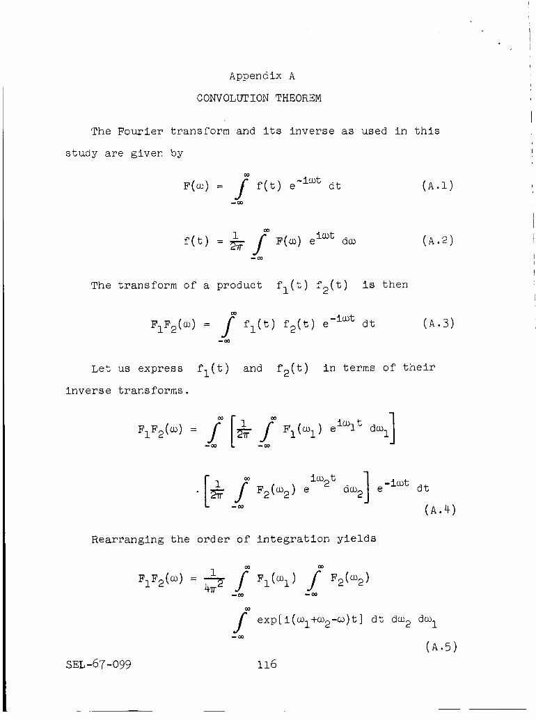
Appendix A
CONVOLUTIONTHEOREM
The Fourier transform and its inverse as used in this
study are given by
F(co) : / f(t) e -i°_t dt (A.I)
i / F(a)) eic°t dco (A 2)f(t): _
The transform of a product fl(t) f2(t) is then
FiF2(co) = / fl(t) f2(t) e -i°°t dt (A.3)
Let us express fl(t)
inverse transforms•
and f2(t) in terms of their
]F1F2(co) : _-_ F l(co I) e d_ 1
/• F2 (co2) e
Rearranging the order of integration yields
SEL -67 -099
i
m_ m_
exp[i(_Ul+CO2-_)t ] dt dco2 dcuImOO
(A.5)ll6

The inside integral over t is identically zero except
where el + _2 - _ = O, where it gives
oo
f exp[i(_l+_2-_)t] dt = 27r$(_i+co2-_ )(A.6)
Then
I
FzF2(oo) = _ f Fl(°' 1)
oo
J" Fa(%) _(%+%-o_) d% _oI
(A.7)
I
FiF2(_o) = >--_- f F 1(%) F2(_-co l) c]% (A.8)
Equation (A.8) expresses the convolution theorem that the
transform of a product is the convolution of the individual
spectra.
The convolution of two functions is often written in
operational notation as
fl(x) (9 f2(x)= f fl(X-y)f2(y)dy (A.9)--00
Using the notation of (A.9) and using a double-headed
arrow to indicate the taking of a transform we may write
fl (t ) -_---_- Fl(CO )
f2(t) _ F2(co )
irl(t ) %(t)-------_ Fl(_) ® F2(_) (A.zo)
117 SEL-67-099

In a similar manner we can obtain
fl (t) (_ f2(t) _FI((O ) F2(co) (A.ii)
SEL-67-099 118

Appendix B
INTERPOLATION
The time-shared real-time algorithm produces each fre-
quency estimate only once for every n input samples. We
have argued that, by looking at only every nth output for
a given frequency, we can obtain all the information that is
present at that frequency. Or to put it another way--if we
have two consecutive estimates (which are n sample times
apart), we can interpolate in some fashion to obtain estimates
for all sample times in between.
From Eq. (i0.i) we can express the time-varying output of
any frequency estimate as
A nf {F(_o,t) : -- F(_) exp -i_[t8_-3
- (n-l)T]}
[ nT ] sin _ (m0 - m)•exp -i -_- (co0 - co) nT - co)_- (_o
(B.I)
At a time nT seconds later the estimate will be
^ n f F(_)exp{-i_[tF(m0, t + nT) = 87+ nT - (n-l)T]}
• exp[-i _ (co0 - co)]
nT - CO)sin -_- (co0
nT_- (_oo - _)
d(1)
(B.2)
119 SEL-67-099

If we assume that the input is a sinusoid that falls
within the 3 dB passband of the filter, then both the input
and output will be of a frequency _0 Z _/nT. The input will
be a simple real sinusoid of this frequency, and the output
will be a complex exponential which rotates at this frequency.
Between t and t + nT the output will rotate Wont _
radians. Recalling that _0 = J2_/nT, we see that the out-
put rotates J complete revolutions + 1/2 revolution. The
rotation of the output is illustrated in Fig. 42.
REAL
IMAGINARY
A A
F(_o,_ /4 F(,,,o,'+k_-)
I//.i / / \
IZ// |,_, 1 /
Fig. 42. ROTATION OF FREQUENCY ESTIMATE OUTPUT.
We can use the computed outputs at times t and t + nT
to interpolate and obtain an output estimate for some time
t + kT in between. We will simply interpolate linearly both
SEL-67-099 120

the magnitude and angle of the output.
the magnitude
Doing so yields for
I$(_o, t + k_)l = I_(_o,t)l + n-_'k_[ i_(_o, t + n_)l - I_(c_o,t) 1]
n n-k I_(_o,t)l + _k i_(COO' t + nT)l (B.3)
The angle of the interpolated output is given by
^ kTLF(_0, t + kT) = LF(_0,t) + _-_ [_0nT +£ F(_ 0, t + nT)
- tg(_o,t) ]
n- k_^ k _$( t + nT) + _0kTF(_o't) + _ _0'n
(B.4)
It should be remembered that the angle of Eq. (B.4) was
arrived at by assuming that the input sinusoid fell within the
3 dB passband of the _0 filter. If it does not, then the
angle of the interpolated frequency estimate will be incorrect.
Since the interpolated output must pass through the points
A
F(_o,t ) and F(_0, t + nT), the angle at time t + nT can
vary only by an integral number of revolutions. Consequently,
at time t + kT the possible errors in angle are
kk 6v k+ 2_ _.., + 4"rr _., + _, ...
Let us use Eq. (I0.i) to express the interpolated output
in terms of the true spectrum.
121 SEL-67-099

I_(%, t + k_)l n - kn
- F(_) exp[-i _ (_0 - c_)]
_I, %z (% _ _)
DT - _)-T (_od_u
k n
/ F(_) exp(-InT_) exp[-i _ (_0 - _)]
sin _ (_0 - _)
DT . _)-T (Wo
n_k
ki/+ _ F(cD) exp[-_. P-_ (c% - c_)]
,jLo
_%T.%T'(_o('"°__)-_)_ (B.5)
It should be noted at this point that the interpolated magni-
tude of the output as given by Eq. (B.5) is obtained by a
nonlinear operation on the input. This means that if we put
in a signal which is the sum of two sinusoids, the output
will not be simply the sum of the individual responses to the
sinusolds. Consequently we cannot define a passband charac-
teristic for the interpolated output as we did for the com-
puted outputs. We can, however, use a single cosine wave to
test and partially define the frequency response of the inter-
polated output. For a cosine wave of frequency e I we have
F(_): _-_(_- %) + _-_(_+ el) (B.6)
SEL-67-099 122

Inserting (B.6) into (B.5) yields
IF(_o,t + k_)l= nS_2-k e_p[-i_ (_o- _l)] n_.r(_o- _i)
+ exp[-i _ (a)0 + C)l)] +
sin_z (_o- _l)k _p[-i_ (_o+ _l)]....." -+ _ n: " _I)_- (_o
sinD{_(_o+ _i)+ exp[-i _ (co0 - c_I)] 'nT ' ' '
In the vicinity of _0 we have
sin _ (_0 -,_l)_i
s____'_(_ +%)-I << I + _I)]-"T o _p[-i_ (<_o _ (_o-%-) 1_p[-i _ (% - _l)] --_ (% + _i) I
(B.Sa)
sln _ (_0 + _i) I << lexP[-i _ (_0" _i)] - nT ,_ _ U_l) |
l_xp[-i_(%+_i )]-__(%+_I) _ -_ o
(B.Sb)
Consequently, near _0 we can write
^ n
IF(_o, t + l<_)l--8-_ nT
-Y (_o - _l)
(B.9)
Similarly, near -_0 we have
nsin +el)
_-(_o + _i)
(B.IO)
123 SEL-67-099

Figure 43 illustrates this magnitude "passband characteristic."
It should be remembered, as mentioned above, that the
interpolated output is the result of a nonlinear operation.
Consequently a true passband characteristic cannot be defined
for it. Figure 43, then, should be thought of only as a first-
order approximation to a passband characteristic.
- _0
Fig. 43. MAGNITUDE "PASSBAND CHARACTERISTIC" OF
INTERPOLATED OUTPUT.
SEL-67-099 124

BIBLIOGRAPHY
Allen, J. L., "The Theory of Array Antennas," TechnicalReport No. 323, M.I.T. Lincoln Laboratory, Cambridge,Mass., 25 Jul 1963.
Aseltine, J. A., Transform Method in Linear System Analysis,McGraw-Hill Book ComPany, New York, 195_.
Bergland, G. D., and H. W. Hale, "Digital Real-Time Spectral
" IEEE Trans Electronic Cgmputerg, EC-I_, 2,Analysis,
Apr 1967.
Bingham, C., M. D. Godfrey, and J. W. Tukey, "Modern Tech-
niques of Power Spectrum Estimation," IEEE Trans. Audioand Electroacoustics, AU-15, 2, Jun 19_7.
Blackman, R. B., and J. W. Tukey, The Measurement of Power
Spectra, Dover Book Company, New York, 1959.
Bogert, B. P., and E. Parzen, "Informal Comments on the Uses
of Power Spectrum Analysis," IEEE Trans. Audio andElectroacoustics, AU-15, 2, Jun 1967.
Bracewell, R. M., The Fourier Transform and Its Applications,McGraw-Hill Book Company, New York, 19_5.
Chu, T., Digital Computer Design Fundamentals, McGraw-Hill
Book Combahy, New York, 19bN.
Cooley, J. W., P. A. W. Lewis, and P. D. Welch, "Historical
Notes on the Fast Fourier Transform," IEEE Trans. Audio
and Electroacoustics, AU-15, 2, Jun 1967a.
Cooley, J. W., P. A. W. Lewis, and P. D. Welch, "Application
of the Fast Fourier Transform to Computation of Fourier
Integrals, Fourier Series, and Convolution Integrals,"
IEEE Trans. Audio and Electroacoustics, AU-15, 2, Jun196'7b.
Cooley, J. W., and J. W. Tukey, "An Algorithm for the Machine
Calculation of Complex Fourier Series," Math. Computation,
19, 90, Apr 1965.
Daley, F. D., Jr., "Analog-to-Digital Conversion Techniques,"
Electro-Technolo_y, May 1967.
Flanagan, J. L., "Spectrum Analysis in Speech Coding," IEEETrans. Audio and Electroacoustics, AU-15, 2, Ju_ 19-_-_.
125 SEL-67-099

G-AE Subcommittee on Measurement Concepts, "What Is the FastFourier Transform?" IEEE Trans. Audio and Electro-
acoustics, AU-15, 2, Jun 19_7.
Gentleman, W. M., and G. Sande, "Fast Fourier Transforms--
for Fun and Profit," AFIPS Fall Joint Computer Conf.Proc., 29, Spartan Books, Washington, D.C., '1906','pp.
Helms, H. D., "Fast Fourier Transform Method of Computing
Difference Equations and Simulating Filters," IEEETrans. Audio and Electroacoustics, AU-15, 2, J_---T967.
Lanczos, C., Applied ANalysis , Prentice-Hall, Inc., EnglewoodCliffs, N.J., 1964.'
Larson, A. G., and R. C. Singleton, "Real-Time Spectral
Analysis on a Small General-Purpose Computer," AFIPS
Fall Joint Computer Conf., Anaheim, Calif., 14-1-_v
1967, to be published in vol. 31 proceedings.
Maling, G. C., Jr., W. T. Morrey, and W. W. Lang, "Digital
Determination of Third-Octave and Full Octave Spectra
of Acoustical Noise, IEEE Trans. Audio and Electro-
acoustic 9, AU-I______5,2, Ju_ 19_7.
Mason, J. J., and H. J. Zimmerman, Electronic Circuits,
Signals, anJ" Systems, John Wiley & Sons, New York, 1960.
Perini, J., "Side-Lobe Reduction Beam Shifting, IEEE Trans.
Antennas and Propagation, AP-12, 6, Nov 1964, pp. 791-792.
Phister, M., Jr., Logical Design of Digital Computers, JohnWiley & Sons, New York, 1958.
"ASingleton, R.C., Method for Computing the Fast Fourier
Transform with Auxiliary Memory and Limited High-Speed
Storage," IEEE Trans. Audio and Electroacoustics,.. AU-15,2, Jun 1967.
Singleton, R, C., "On Computing the Fast Fourier Transform,"
Research Memorandum, Mathematical Sciences Department,
Stanford Research Institute, Menlo Park, Calif., Jul1967.
Singleton, R. C., and T. C. Poulter, "Spectral Analysis of
the Call of the Male Killer Whale," IEEE Trans. Audio
and Electroacousti.c9 , AU-15, 2, Jun 1967.
SEL-67-099 126

"An Introduction to Time Series Analysis,Sloane, E. A.,Time/Data Corporation, Palo Alto, Calif., Mar 1967.
Weaver, C. S., P. E. Mantey, R. W. Lawrence, and C. A. Cole,"Digital Spectrum Analyzers," Report SU-SEL-66-059(TR 1809/1810-1), Stanford Electronics Laboratories,Stanford, Calif., Jun 1966.
Welch, L. R., "Computation of Finite Fourier Series," JPLSpace Programs Summary No. 37-37, IV, Jet PropulsionLaboratory, Pasadena, Calif., Jan 966.
Welch, P. D., "The Use of the Fast Fourier Transform for theEstimation of Power Spectra: A Method Based on TimeAveraging over Short, Modified Periodograms," IEEETrans ,. Audio and Electroacousticg, AU-15, 2, J_--T967.
127 SEL-67-099