A Primer for EOF Analysis of Climate

Data

A. Hannachi

Department of Meteorology, University of Reading

Reading RG6 6BB, U.K.

email: A.Hannachi@reading.ac.uk

March 24, 2004

1

Contents

1 Introduction 3

2 Structure of climate data 4

2.1 Data matrix . . . . . . . . . . . . . . . . . . . . . . . . . . . . . . . . 4

2.2 Area weighting . . . . . . . . . . . . . . . . . . . . . . . . . . . . . . 5

3 Empirical orthogonal functions 5

3.1 Historical overview . . . . . . . . . . . . . . . . . . . . . . . . . . . . 5

3.2 Derivation and use of EOFs . . . . . . . . . . . . . . . . . . . . . . . 6

3.2.1 Derivation of EOFs . . . . . . . . . . . . . . . . . . . . . . . . 6

3.2.2 Use of EOFs . . . . . . . . . . . . . . . . . . . . . . . . . . . . 7

3.3 Computational aspects . . . . . . . . . . . . . . . . . . . . . . . . . . 8

3.4 Interpretation of EOFs . . . . . . . . . . . . . . . . . . . . . . . . . . 10

3.5 Application . . . . . . . . . . . . . . . . . . . . . . . . . . . . . . . . 10

4 Rotated empirical orthogonal functions 12

4.1 What is it and why? . . . . . . . . . . . . . . . . . . . . . . . . . . . 12

4.2 Derivation of REOFs . . . . . . . . . . . . . . . . . . . . . . . . . . . 13

4.3 Application . . . . . . . . . . . . . . . . . . . . . . . . . . . . . . . . 13

5 Extended empirical orthogonal functions 15

5.1 Introduction . . . . . . . . . . . . . . . . . . . . . . . . . . . . . . . . 15

5.2 Extended EOFs . . . . . . . . . . . . . . . . . . . . . . . . . . . . . . 15

5.2.1 Historical overview . . . . . . . . . . . . . . . . . . . . . . . . 15

5.2.2 Definition of EEOFs . . . . . . . . . . . . . . . . . . . . . . . 15

5.2.3 Computation of EEOFs . . . . . . . . . . . . . . . . . . . . . 17

5.3 Data filtering and oscillation reconstruction . . . . . . . . . . . . . . 18

5.4 Application to outgoing long wave radiation . . . . . . . . . . . . . . 19

6 Summary and conclusion 29

2

1 Introduction

Climate is regarded as the aggregation of (random) daily weather, and as pointed

out by Lorenz (1970), climate is what we expect but weather is what we get. As

such, climate is considered as the long term statistics of weather. Climate variations

are also the result of exceedingly complex nonlinear interactions between very many

degrees of freedom or modes. Despite being the statistics, or averages, of weather

climate is still characterised by nonlinearity and high dimensionality. Consequently,

a challenging task is to find ways to redue the dimensionality of the system and find

the most important patterns explaining the variations. In the last several decades,

meteorologists have in fact put major efforts in extracting important patterns from

measurements of atmospheric variables. As a result Empirical Orthogonal Functions

(EOF) technique has become the most widely used way to do this and the present

primer is a guide for the same purpose.

The original purpose of EOFs was to reduce the large number of variables of the

original data to a few variables, but without compromising much of the explained

variance. Lately, however, EOF analysis has been used to extract individual modes of

variability such as the Arctic Oscillation (AO), (Thompson and Wallace 1998, 2000)

known as teleconnections (Angstrom 1935; Bjerknes 1969; Wallace and Gutzler 1981,

etc.). EOFs are presented in section 2.

The simplicity and the analytic derivation of EOFs are the main reasons behind

its popularity in atmospheric science. The physical interpretability of the obtained

patterns is, however, a matter of controversy because of the strong constraints satisfied

by EOFs, namely orthogonality in both space and time. Physical modes such as

normal modes (Simmons et al. 1983) are not in general orthogonal. This shortcoming

has led to the development of rotated empirical orthogonal functions (REOFs), see

Richman (1986). REOFs yields in general localised structures by compromising some

of the EOFs properties such as orthogonality. REOFs will be presented in section 3.

EOFs and REOFs are mainly based on using the spatial correlation of the field,

an important feature of climate data. Auto- and cross-correlation in time between

grid points are, however, ignored in those techniques. Extended EOFs (Weare and

Nasstrom, 1982) is a technique that attempts to incorporate both the spatial and the

temporal correlation. The method has since become a useful tool to extract dynamical

structure, trends and oscillations, and to filter data. EEOFs will be presented in

section 5.

3

2 Structure of climate data

2.1 Data matrix

Gridded climate data normally come as an array containing for each vertical level

a three-dimensional, two-dimensional in space and one-dimensional in time, field F .

The latter is a function of time t, latitude θ, and longitude φ. We suppose that

the horizontal coordinates are discretised to yield latitudes θj , j = 1, . . . , p1, and

longitudes φk, k = 1, . . . p2, and similarly for time, i.e. ti, i = 1, . . . n. This yields a

total number of grid points p = p1p2. The discretised field reads:

Fijk = F (ti, θj , φk) (1)

with 1 ≤ i ≤ n, 1 ≤ j ≤ p1, and 1 ≤ k ≤ p2. It is in general tedious and memory-

consuming to process three- and higher-dimensional arrays such as F . We therefore

transform F into a two-dimensional array: the data matrix X where the two spatial

dimensions are concatenated together. This is achieved using the MATLAB cammand:

>> [n, p1, p2] = size (F);

>> X = reshape (F, n, p1*p2);

We now suppose that we have a gridded data set composed of a space-time field X(t, s)

representing the value of the field X, such as SLP, at time t and spatial position s.

The value of the field at discrete time ti and grid point sj is noted xij for i = 1, . . . , n

and j = 1, . . . p = p1p2. The observed field is then represented by the data matrix:

X =

x11 x12 . . . x1p

x21 x22 . . . x2p

......

...

xn1 xn2 . . . xnp

(2)

If we denote by x.j the time average of the field1 at the j’th grid point, i.e.

x.j =1

n

n∑

k=1

xkj (3)

then the climatology of the field is defined by

x = (x.1, . . . , x.p)

1The seasonal and other external, e.g. diurnal cycles are supposed to have been removed from

the data.

4

The anomaly field, or departure from the climatology is defined at (t, s) by:

x′

ts = xts − x.s

or in matrix form:

X ′ = X − 1x =

(

I −1

n11T

)

X (4)

where 1 = (1, . . . 1)T is the (column) vector containing n ones, and I is the n × n

identity matrix. If X is the original data matrix, then the MATLAB commands to

calculate the anomaly are:

>> [n,p] = size (X);

>> Xbar = mean (X,1);

>> Xprime = X - ones(n,1) * Xbar;

2.2 Area weighting

Most climate data whether observed or model-simulated are in general non-uniformly

distributed over the Earth surface. For example, if the data are provided on a grid

with 5olat×5olon resolution, then clearly the distribution of the data will be denser

poleward. This non-uniform distribution can influence the structure of the computed

EOFs. In order to avoid the effect of this geometrical artifact we normally weigh the

data prior to analysing them. The simplest and most useful way is to weigh each data

point by the local area of its location. Hence each datum is weighted by the cosine

of its latitude. Let us designate by θk the latitude of the k’th grid point, k = 1, . . . p,

and Dθ the diagonal matrix:

Dθ = Diag [cosθ1, . . . , cosθp] (5)

Then the weighted anomaly matrix is

Xw = X ′Dθ. (6)

3 Empirical orthogonal functions

3.1 Historical overview

Empirical Orthogonal Function technique aims at finding a new set of variables that

capture most of the observed variance from the data through a linear combination of

the original variables. Empirical Orthogonal Functions (EOFs) have been introduced

in atmospheric science since the early 50’s, e.g. Obukhov (1947, 1960), Fukuoka

5

(1951), Lorenz (1956), see also Craddock (1973) for a discussion on relevant prob-

lems in analysing multivariate data in meteorology. The EOF terminology is due to

Lorenz (1956) who applied it in a forecasting project at the Massachusetts Institute of

Technology. Since then EOFs have become popular analysis tools in climate research.

EOF techniques are deeply rooted in statistics, and go back to Hotelling (1933) who

introduced principal component analysis (PCA), another name for EOFs. A review

of PCA/EOFs can be found in Kutzbach (1967). EOFs, however, are not restricted

to multivariate statistics or atmospheric sciences. They extend to the analysis of

stochastic fields in the mathematical literature where they are known under the name

Karhunen-Loeve basis functions (Loeve 1978). Detailed analyses of EOFs can be

found for example in Wilks (1995), von Storch and Zwiers (1999), and Jolliffe (2002).

3.2 Derivation and use of EOFs

3.2.1 Derivation of EOFs

We present below a brief description of EOFs, and for more details the reader is

referred, for example, to Kutzbach (1967), Wilks (1995), Storch (1993), Storch and

Zwiers (1999), and Joliffe (2002). Once the anomaly data matrix (4) or its weighted

version (6) is determined, the covariance matrix is then defined by:

Σ =1

n − 1X

′T X ′, (7)

which contains the covariance between any pair of grid points. The aim of EOF/PCA

is to find the linear combination of all the variables, i.e. grid points, that explains

maximum variance. That is to find a direction a = (a1, . . . , ap)T such that X ′a has

maximum variability. Now the variance of the (centered) time series X ′a is

var (X ′a) =1

n − 1‖X ′a‖2 =

1

n − 1(X ′a)

T(X ′a) = aT Σa

To make the problem bounded we normally require the vector a to be unitary. Hence

the problem readily yields:

maxa

(

aT Σa)

, s.t. aTa = 1 (8)

The solution to (8) is a simple eigenvalue problem (EVP):

Σa = λa. (9)

By definition the covariance matrix Σ is symmetrical and therefore diagonalisable.

The k’th EOF is simply the k’th eigenvector ak of Σ after the eigenvalues, and the

6

corresponding eigenvectors, have been sorted in decreasing order. The covariance

matrix is also semidefinite, hence all its eigenvalues are positive. The eigenvalue

λk corresponding to the k’th EOF gives a measure of the explained variance by ak,

k = 1, . . . p. It is usual to write the explained variance in percentage as:

100λk∑p

k=1 λk

%

The projection of the anomaly field X ′ onto the k’th EOF ak, i.e. ck = X ′ak is the

k’th principal component (PC)

ck(t) =

p∑

s=1

x′(t, s)ak(s) (10)

3.2.2 Use of EOFs

Because Σ is diagonalisable the set of its eigenvectors forms an orthogonal basis of the

p-dimensional Euclidean space, defined with the natural scalar product. So by con-

struction, the Empirical Orthogonal Functions are orthogonal and the PCs uncorre-

lated. This completely characterises conventional EOFs. The orthogonality property

provides a complete basis where the time-varying field can be separated as:

X ′(t, s) =M∑

k=1

ck(t)ak(s) (11)

This property constitutes, however, a strong constraint that puts limits to the physical

interpretability of individual EOFs since in general physical patterns tend to be non-

orthogonal (Simmons et al. 1983).

Furthermore, The eigenvalues of Σ are not necessarily distinct and some may have

multiplicity greater than one, i.e. degenerate. Therefore, the separation between

eigenvalues can be problematic when two or more eigenvalues are degenerate. The

investigation of the degeneracy of the covariance matrix spectrum requires a measure

of uncertainty of each eigenvalue that reflects sampling and this is quite difficult to get.

In practice there are mainly two ways to compute the uncertainty of the eigenvalues

and/or the eigenvectors of Σ. The first one, which is used here, is based on a rule of

thumb (North et al. 1982):

∆λk ≈ λk

√

2n

∆ak ≈ ∆λk

λj−λkaj

(12)

where λj is the closest eigenvalue to λk, and n is the sample size2. Alternatively, one

can use Monte Carlo simulations. This can be achieved by forming surrogate data by

2To be more precise n is the number of independent data in the sample

7

resampling a part of the data using randomisation3.

Another drawback of EOFs comes when we use them to reduce the dimensionality

of the data, namely the truncation order that can be applied to the sum (11). In prac-

tice the truncation order is obtained by fixing the amount of explained variance, e.g.

80%, and choose the leading EOFs that explain altogether this amount of variance.

3.3 Computational aspects

In practice we do not need to solve the EVP (9). We use a powerful tool from linear

algebra namely singular value decomposition (SVD), (e.g. Linz and Wang 2003) to

factor any p × n matrix Y (7) as4:

Y = LΛRT (13)

where L is a p × p matrix containing the left singular vectors, R is n × n matrix

containing the right singular vectors, and Λ is a diagonal matrix of the same dimension

as Y , i.e. p×n, with nonnegative diagonal elements. These elements are the singular

values. Note that the maximum number of nonzero singular values is M = min(n, p),

the rank of the matrix Y . The matrices L and R are both orthonormal, or unitary,

in the sense that LT L = LLT = IM and similarly for R.

In meteorological application we take Y = X ′T when p ≤ n. The EOFs are

provided by the columns of L and the PCs by the columns of R. The MATLAB

application is obtained as

>> Fprime = reshape (Xprime, n, p1, p2);

>> [eofs, pcs, var] = eofsvd (Fprime, 1, lat, 20);

where an area weighting is applied by the argument ’1’ and we retained the first 20

EOFs. Note that the first and the second columns of ”var” provide respectively the

eigenvalues of the covariance matrix and the explained varainces (%) of the EOFs. To

plot the spectrum of the data covariance matrix along with their uncertainties use:

>> eigenplot (Xprime, var(:,2))

3An example would be to randomly select a subsample and apply EOFs, then select another

subsample etc. This operation can be repeated many times, which yields various realisations of

the eigenelements of the resulting covariance matrix from which one can estimate the uncertainties.

Another example would be to fix a subset of variables then scramble them by permuting the data,

i.e. breaking the chronological order then apply EOFs, and so on.4In (11) we suppose that p ≤ n, otherwise we get p−n zero singular values. In this case, i.e. when

p > n we normally transpose the matrix Y and apply SVD to get efficient (fast) decomposition.

8

0 10 20 30 40 500

5

10

15

20

25

30

Eigenvalue spectrum

Rank

Eig

enva

lue

(%)

Figure 1. The spectrum of the covariance matrix showing the first 50 eigenvalues

(%), i.e. explained variance of the the first 50 EOFs.

9

3.4 Interpretation of EOFs

By construction EOFs constitute directions of variability with no particular ampli-

tude. Therefore if l is an EOF, so is αl for any nonzero α. For convenience, however,

they are chosen to be unitary. Also by construction EOFs are stationary structures,

i.e. they do not evolve in time. The principal component attached to the correspond-

ing EOF provides the sign and the overall amplitude of the EOF as a function of time.

This provides a simplified representation of the state of the field at that time along

that EOF. In other words EOFs do not change structure in time, they only change

sign and overall amplitude to represent the state of the atmosphere. When EOFs are

nondegenerate they can be studied individually. When they are degenerate, however,

the separation between them becomes problematic despite being orthogonal and their

PCs uncorrelated.

Although EOFs represent patterns that (successively) explain most of the observed

variability, their interpretation is, however, not always simple. Physical interpretabil-

ity especially can be controversial, see e.g. Dommenget and Latif (2002). For physical

modes are not necessarily orthogonal (Simmons et al. 1983). The constraints imposed

upon EOFs are purely geometric and hence can be non-physical. Furthermore, the

EOF structure tends to be domain dependent (Richman 1986) and this adds to the

difficulty of their physical interpretability. These arguments constitute the main rea-

sons for attempts to find ways round EOFs. The method of rotated EOFs, which is

presented below, constitutes one way.

3.5 Application

We have applied EOFs to the winter monthly SLP over the Northern Hemisphere

(NH). The data come from the National Center for Atmospheric Research and Na-

tional Center for Environmental Prediction (NCAR/NCEP) from 1948 to 2000 on a

regular horizontal grid with 2.5o × 2.5o resolution. The winter season is defined by

December to February (DJF). The seasonal cycle is first calculated as monthly av-

eraged values then removed from the data. Finally a weighting by the cosine of the

corresponding latitude is applied. The data over the NH north of 20oN is used to

compute EOFs.

Figure 1 shows the spectrum of the covariance matrix along with their uncertain-

ties using approximation (12). The first eigenvalue seems separated from the rest,

but overall the spectrum looks in general continuous, which makes truncation diffi-

cult. The first two EOFs (Fig. 2) explain respectively 21% and 13% of the total

variance. EOF 1 shows a high over the North Pole and two low centres over the

10

−14−12−10 −8 −6 −4 −2 0 2 4 6 8 10 12 14 16 18 20 22 24 26 28 30

−14−12−10 −8 −6 −4 −2 0 2 4 6 8 10 12 14 16 18 20 22 24 26 28 30

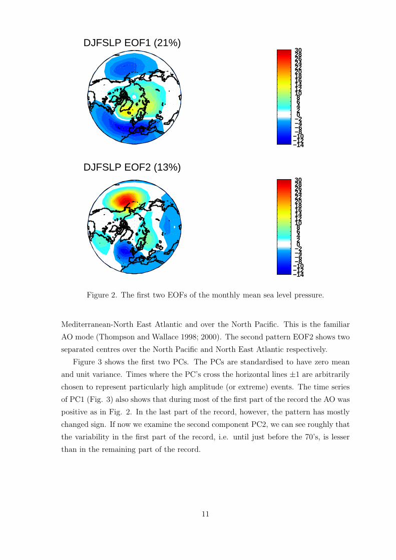
DJFSLP EOF1 (21%)

DJFSLP EOF2 (13%)

Figure 2. The first two EOFs of the monthly mean sea level pressure.

Mediterranean-North East Atlantic and over the North Pacific. This is the familiar

AO mode (Thompson and Wallace 1998; 2000). The second pattern EOF2 shows two

separated centres over the North Pacific and North East Atlantic respectively.

Figure 3 shows the first two PCs. The PCs are standardised to have zero mean

and unit variance. Times where the PC’s cross the horizontal lines ±1 are arbitrarily

chosen to represent particularly high amplitude (or extreme) events. The time series

of PC1 (Fig. 3) also shows that during most of the first part of the record the AO was

positive as in Fig. 2. In the last part of the record, however, the pattern has mostly

changed sign. If now we examine the second component PC2, we can see roughly that

the variability in the first part of the record, i.e. until just before the 70’s, is lesser

than in the remaining part of the record.

11

Jan40 Jan50 Jan60 Jan70 Jan80 Jan90 Jan00 Jan10−3

−2

−1

0

1

2

3

Time

PC

1

DJF SLP PC1

Jan40 Jan50 Jan60 Jan70 Jan80 Jan90 Jan00 Jan10−3

−2

−1

0

1

2

3

Time

PC

2

DJF SLP PC2

Figure 3. The first two PCs of the monthly mean sea level pressure.

4 Rotated empirical orthogonal functions

4.1 What is it and why?

Rotated EOF (REOF) is a technique simply based on rotating EOFs. REOF tech-

niques have been adopted by atmospheric scientists since the mid-eighties as an at-

tempt to overcome some of the previous shortcomings such as the difficulty of physical

interpretability. The technique, however, is much older and goes back to the early

fourties (Thurstone 1940, 1947; Caroll 1953). The technique is also known in factor

analysis as factor rotation and aims at getting simple structures. In meteorology the

objective was to

• alleviate the strong constraints of EOFs, namely orthogonality/uncorrelation of

EOFs/PCs, domain dependence of EOF patterns (see e.g., Dommengent and Latif

2002),

• obtain simple structures, and

• be able to physically interpret the patterns.

12

4.2 Derivation of REOFs

Here one seeks a rotation matrix Q to construct the rotated EOFs U according to:

U = LQ (14)

where L = [l1, l2, . . . lm] is the matrix of the leading m EOFs (or loadings). The

criterion for choosing the m × m rotation matrix Q is what constitutes the rotation

algorithm, which is expressed by the minimization problem:

min f (LQ) (15)

over a specified subset of square rotation matrices Q. The functional f represents the

rotation criterion. Various rotation criteria exist in the literature. Richman (1986), for

example, lists five simplicity criteria. Broadly speaking there are two large families of

rotation namely, orthogonal and oblique rotations. In the former the rotation matrix

Q in (14) is chosen to be orthogonal, and the problem is to solve (15) subject to the

orthogonality condition:

QQT = QT Q = I. (16)

By contrast, in the latter case the rotation matrix Q is non-orthogonal.

The most well known and used rotation algorithm is the varimax criterion (Kaiser

1958). It is an orthogonal rotation based on the criterion:

max

m∑

k=1

p

p∑

j=1

u4ij −

(

p∑

j=1

u2jk

)2

(17)

where U = (uij), and m is the number of EOFs chosen for rotation. The quantity

inside the square brackets in (17) is proportional to (spatial) variance of the square of

the rotated vector uk = (u1k, . . . , upk)T . Therefore the varimax attempts to simplify

the structure of the patterns by tending the loadings towards zero, or ±1. The

MATLAB command to do REOFs is

>> U = roteofs (eofs, m)

4.3 Application

In this manuscript we have applied the varimax rotation to the SLP for various values

of the number m of retained EOFs. Fig. 4 shows the first two rotated EOFs for

m = 10 (first row) and m = 20 (2nd row) retained EOFs respectively. For small m

(m ≤ 15) REOF1 shows a clear NAO pattern, a dipolar structure, with the strongest

centre located over Greenland and REOF2 shows the Pacific pattern centered around

13

-5-4-3-2-1 0 1 2 3 4 5 6 7 8 910

-5-4-3-2-1 0 1 2 3 4 5 6 7 8 910

-5-4-3-2-1 0 1 2 3 4 5 6 7 8 910

-5-4-3-2-1 0 1 2 3 4 5 6 7 8 910

REOF1 (m=10) REOF2 (m=10)

REOF1 (m=20) REOF1 (m=20)

Figure 4. The first two rotated EOFs using 10 (first row) and 20 (2nd row) EOFs

respectively.

the Aleutian (Fig 4). As m increases the centre over Western Europe/Eastern At-

lantic of REOF1 diminishes and eventually vanishes for m ≥ 25 and we are left with

a very localised centre east of Greenland. Similarly, the Pacific centre of REOF2

becomes very localised. Note that if the EOFS are not area-weighted then REOF1

becomes localised over the North Pole instead of Greenland (not shown). Rotated

EOFs therefore yield localised or simple structures, but they are dependent on the

number of retained EOFs.

REOFs, like EOFs, also suffer some drawbacks, namely criterion choice, and the

number of retained EOFs. In addition the (EOF) property of successive variance

maximisation is lost during the rotation process. This yields patterns that do not

constitute the main source of variation. Joliffe et al. (2002), for example, pointed to

the difficulty in building a criteria to take account of various types of simplicity, e.g.

concentration versus equal loadings.

14

5 Extended empirical orthogonal functions

5.1 Introduction

Weather and climate data have beside their large dimensionality a high correlation

in space and also significant correlation in time. EOFs constitute a basic and useful

tool to learn about large scale patterns that explain most of the variability. Since

EOFs find the combination of variables which explain most of the variability it is

implied, in particular, that EOFs make use of the usually observed high correlation in

space. The significant correlation in time is, however, not taken into account. Auto-

and cross-correlation in time can be very useful for prediction purposes and also for

building probabilistic time series models. Extension of EOFs to deal with correlation

in time also exist and is presented below.

5.2 Extended EOFs

5.2.1 Historical overview

Extended empirical orthogonal functions (EEOFs) constitute an extension of the tra-

ditional EOF technique to deal not only with spatial- but also with temporal corre-

lations observed in weather/climate data. The method has been first introduced by

Weare and Nasstrom (1982) who applied it to the 300-mb relative vorticity.

Similar approach has been developed later to deal with dynamical reconstruction

of low order chaotic systems by Broomhead and King (1986a,b) who called it singular

system analysis (SSA) in the unidimensional case. At the same time Fraedrich (1986)

also used the same approach to compute dimensions of chaotic attractors from climate

data. SSA was also used to find oscillations from climate records (Vautard et al.

1992). It has been extended to deal with multivariate, or multichannel, (MSSA) time

series (Broomhead and King 1986a,b) in a way similar to EEOF. MSSA (EEOF)

was applied later by Kimoto et al. (1991) and Plaut and Vautard (1994) to find

propagating structures from observed 500-mb heights.

5.2.2 Definition of EEOFs

In EEOF the atmospheric state vector at time t, i.e. xt = (xt1, . . . xtp), t = 1, . . . , n,

used in traditional EOF, is extended to include temporal information as

xt = (xt1, . . . xt+M−1,1, xt2, . . . xt+M−1,2, . . . xt,p, . . . xt+M−1,p) (18)

15

with t = 1, . . . , n−M + 1. The parameter M used in (18) is known as window length

or delay parameter5. The new data matrix takes now the form

X =

x1

x2

...

xn−M+1

(19)

It is now clear from (18) that time is incorporated in the state vector side by side

with the spatial dimension. If we denote by

xst = (xts, xt+1,s . . . xt+M−1,s) (20)

then the extended state vector (18) is written in a similar form to the conventional

state vector, i.e.

xt =(

x1t , x

2t , . . . , x

pt

)

(21)

The data matrix X in (19) now takes the form

X =

x11 x

21 . . . x

p1

......

...

x1n−M+1 x

2n−M+1 . . . x

pn−M+1

(22)

which is similar to traditional data matrix X in (2) except that now its elements are

vectors.

The vector xst in (20) is normally referred to as the delayed vector obtained from the

time series (xst ), t = 1, . . . n of the field value at grid point s. The new data matrix

(22) is now of order (n − M + 1) × pM which is significantly larger than the original

matrix dimension.

We suppose that X in (22) has been centered and weighted etc. The covariance

matrix of (22) is

Σ =1

n − M + 1X TX =

C11 C12 . . . C1M

C21 C22 . . . C2M

......

...

CM1 CM2 . . . CMM

(23)

where each Cij, 1 ≤ i, j ≤ M is a lagged covariance matrix between gridpoint i and

gridpoint j given by6

Cij =1

n − M + 1

n−M+1∑

k=1

xik

Tx

jk (24)

5also known as embedding dimension. This concept is rooted in the theory of dynamical systems.6Other alternatives to compute Cij also exist and they are related to the way the lagged covariance

between two time series is computed.

16

If the elements of the data matrix (22) were random variables and where the covariance

matrix is Σ = E(

X TX)

, then each submatrix Cij = E(

xiT

xj)

will exactly take a

symmetric Toeplitz form, i.e. with constant diagonals and consequently Σ will be bloc

Towplitz. Due to finite sampling, however, Cij is approximately Toeplitz for large

values of n (compared to the window length M). This is in general the case when we

deal with high frequency data, e.g. daily observations or even monthly averages from

climate models. The covariance matrix Σ is therefore a symmetric approximately

bloc-Toeplitz for large values of n. Alternative form of the data matrix is provided

by writing the state vector (18) in the form

xt = (xt1, . . . xt,p, xt+1,1, . . . xt+1,p, . . . xt+M−1,1, . . . xt+M−1,p) (25)

that is

xt = (xt,xt+1, . . . ,xt+M−1) (26)

where xt is the state vector at time t, t = 1, . . . n − M + 1, i.e.

xt = (xt1 . . . xt,p) .

Hence the matrix (22) now takes the alternative form7

X1 =

x1 x2 . . . xM

......

...

xn−M+1 xn−M+2 . . . xn

(27)

This form is exactly equivalent to (22) since it is obtained from (22) by a permutation

of the columns as

X1 = XP (28)

where P = (pij), i, j = 1, . . .Mp, is a permutation matrix8 given by

pij = δi,α (29)

where α is a function of j given by α = rM +[

j

p

]

+ 1 where j − 1 ≡ r(p), and [x] is

the integer part of x.

5.2.3 Computation of EEOFs

EEOFs are the EOFs of the extended data matrix (19), i.e. the eigenvectors of the

grand covariance matrix Σ given in (23). They can be obtained directly by computing

7used by Weare and Nasstrom 19828which contains exactly 1 in every line and every column and zeros elswhere. A permutation

matrix P is orthogonal, i.e. PPT = PT P = I.

17

the eigenvalues/eigenvectors of (23). Alternatively, we can use again the SVD of the

grand data matrix X in (22) in a similar way to (13). This yields

X = V ΘUT (30)

where U = (uij) = (u1, u2, . . . , ud) represents the matrix of the d extended EOFs

or left singular vectors of X , where d = Mp represents the number of new vari-

ables, i.e. the number of columns of the grand data matrix. The diagonal matrix

Θ contains the singular values θ1, . . . θd of X , and V = (v1, v2, . . . , vd) is the ma-

trix of the right singular vectors or extended PC’s, i.e. the k’th extended PC is

vk = (vk(1), . . . , vk(n − M + 1))T . These extended EOFs and PCs can be used to

filter the data by removing the contribution from nonsignificant components or for

reconstruction purposes as detailed below

5.3 Data filtering and oscillation reconstruction

The extended EOFs U can be used as a filter exactly like EOFs. For instance the

SVD decomposition (30) yields the expansion of each row xt of X in (22)

xTt =

d∑

k=1

θkvk(t)uk (31)

for t = 1, . . . n − M + 1, or in terms of the original variables xt as

xTt+j−1 =

d∑

k=1

θkvk(t)ujk (32)

for t = 1, . . . n − M + 1, and j = 1, . . .M , and where

ujk =

(

uj,k, uj+M,k, . . . , u(p−1)M,k

)T.

Note that the expression of the vector ujk depends on the form of the data matrix.

The one given above corresponds to (22), whereas for the data matrix X1 (27) we get

ujk =

(

u(j−1)p+1,k, u(j−1)p+2,k, . . . , ujp,k

)T

Note that when we filter out high ranked EEOFs expression (32) is to be truncated

to the required order d1 < d.

The expansion (32) is exact by construction. However, when we truncate it by

keeping a smaller number of EEOFs for filtering purposes, e.g. when we reconstruct

the field components from a single EEOF or a pair of EEOFs corresponding for ex-

ample to an oscillation, then the previous expansion does not give a complete picture.

This is because (32) truncated to a smaller subset K of EEOFs, e.g.

yTt+j−1 =

∑

k in K

θkvk(t)ujk (33)

18

where yt = (yt,1, . . . , yt,p) is the filtered or reconstructed state space vector, becomes

a multivalue function. For example, for t = 1 and j = 2, we get one value of yt,1 and

for t = 2 and j = 1 we get another value of yt,1. Note that this is due to the fact

that the EEOFs have time lagged components. To get a unique recontructed value

we simply take the average of those multiple values. The number of multiple values

depends9 on the value of time t = 1, . . . n. The reconstructed variables using a subset

K of EEOFs are then easily obtained from (33) by

yTt =

1t

∑t

j=1

∑

K θkvk(t − j + 1)ujk for 1 ≤ t ≤ M − 1

1M

∑M

j=1

∑

K θkvk(t − j + 1)ujk for M ≤ t ≤ n − M + 1

1n−t+1

∑M

j=t−n+M

∑

K θkvk(t − j + 1)ujk for n − M + 2 ≤ t ≤ n

(34)

Note that these constructions can also be obtained in a least square sense (see, e.g.

Vautard et al. 1992, and Ghil et al. 2001). the reconstructed components can also

be restricted to any subset of the eigen elements of the grand data matrix (22) or

similarly the grand covariance matrix Σ. For example to reconstruct the time series

associated with an oscillatory eigen elements, i.e. a pair of degenerate eigenvalues,

the subset K in the sum (34) is limited to that pair.

The reconstructed multivariate time series yt, t = 1, . . . n, can represent the recon-

structed (or filtered) values of the original field at the original p grid points. In general,

however, the number of grid points is too large to warrant an eigen-decomposition of

the grand data or covariance matrix. In this case a dimension reduction of the data

is first applied by using the p0, say, leading PCs then apply a MSSA to these retained

PCs. In this case the dimension of X becomes (n−M +1)×Mp0, which may be made

considerably smaller than the original dimension. To get the reconstructed space-time

field one then use the reconstructed PCs in conjunction with the p0 leading EOFs.

5.4 Application to outgoing long wave radiation

The outgoing long wave radiation (OLR) comes from NCAR/NCEP reanalyses over

the tropical region from 30oS to 30oN. This analysis focuses on a 5-year period of

daily data from 1 Jan 1996 to 31 Dec 2000. Figure 5 displays the OLR field on 25 Dec

1996. Note the low-value regions particularly over the warm pool, an area of large and

intensive convection, and to a lesser extent over the Amazonian and tropical African

9These numbers can obtained by constructing a M ×n array A = (ajt) with entries ajt = t−j+1.

Next all entries that are nonpositive or greater than n− M + 1 are to be equated to zero. Then for

each time t take all the indices j with positive entries.

19

0° 60° E 120° E 180° E 120° W 60° W 0° 30° S

0°

30° N

94111128145162179196213230247264281298315

OLR on the 25-Dec-1996 (w m-2)

Figure 5. The distribution of OLR (w/m2) on the 25-Dec-1996 over the tropics.

regions. The OLR data is not very homogeneous, and have a quite complicated

variability as well as seasonality. To illustrate this complication, figure 6 shows the

OLR time series at four different locations. A clear indication of nonstationarity of

the times series is obvious. Note for example the high values at the equator and

122.5oE in winter 97/98. This period corresponds to a strong El-Nino event where

the convection shifts eastward to the mid-Pacific allowing more long wave radiation to

be lost to space over the maritime continent. Note also the strong seasonal component

at 30oN.

Before applying EEOF analysis, the data were first subjected to an EOF analysis.

The leading 10 EOFs/PCs of the anomaly field with respect to the long term average

(climatology) were retained for the analysis. Figure 7 shows the leading EOF mode.

This pattern explains about 15% of the total variability and is associated with the

seasonal cycle. Fig. 7 clearly indicates that the seasonal cycle is mostly explained by

the Inter Tropical Convergence Zone (ITCZ) and some monsoonal activities.

The first 10 EOFs/PCs used for the EEOF/MSSA analysis explain altogether

about 32% of the total variability. A window length corresponding to M = 80 days

is used to construct the grand data matrix (22). This choice was motivated by the

desire to capture the Madden-Julian Oscillation (MJO) identified first by Madden and

Julian (1971). The extended (grand) data matrix is then factorised using SVD. Figure

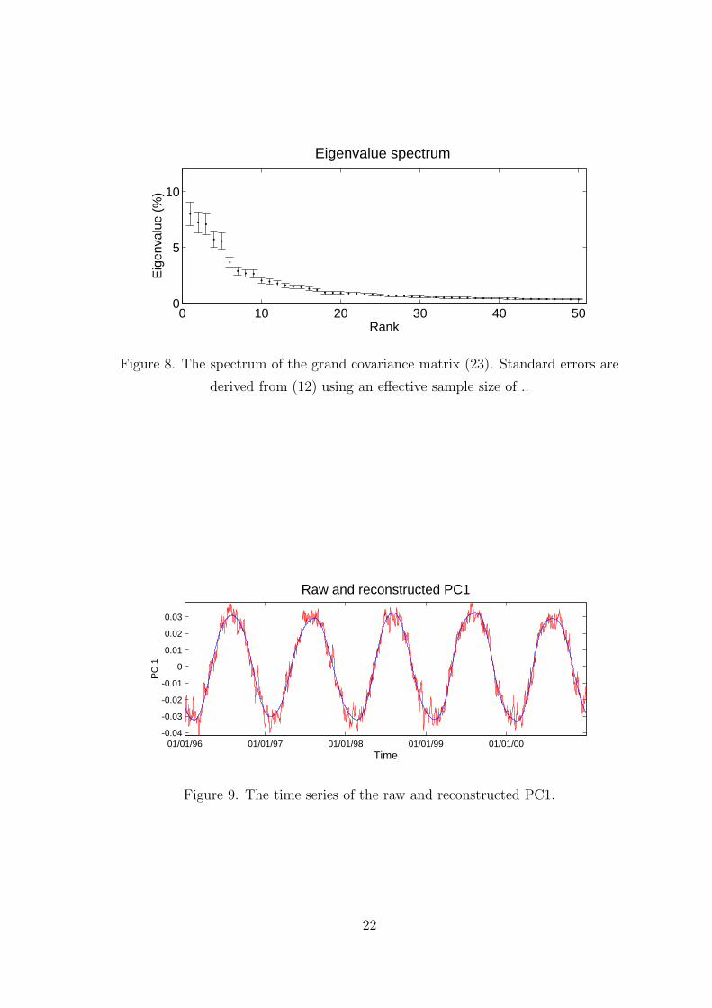
8 shows the spectrum of the grand covariance matrix Σ (23), i.e. the square of the

singular values of the grand data matrix (22). The standard error are obtained using

(12) with a heuristic effective sample size of 116 corresponding to an uncorrelation

lag of 15 days. This is just a rough and heuristic estimation because the observation

period is not long enough.

The first two eigenvalues of the spectrum (Fig. 8) correspond to the oscillation of

the seasonal cycle. They do not look nearly equal and well separated from the rest

20

100

200

300

OLR

(w

m-2

)

OLR (Equator, 122.5oE)

100

200

300

OLR

(w

m-2

)

OLR (Equator, 20oW)

100

200

300

OLR

(w

m-2

)

OLR (Equator, 117.5oW)

01/01/96 01/01/97 01/01/98 01/01/99 01/01/00 01/01/01100

200

300

400

Time

OLR

(w

m-2

)

OLR (30oN, 40oE)

Figure 6. Time series of OLR (wm−2) at four different locations.

0° 60° E 120° E 180° E 120° W 60° W 0° 30° S

0°

30° N

-6

-5

-4

-3

-2

-1

0

1

2

3

4

5EOF1 of OLR 1996-2000

Figure 7. The leading EOF of OLR anomalies. Units are arbitrary.

21

0 10 20 30 40 500

5

10

Eigenvalue spectrum

Rank

Eig

enva

lue

(%)

Figure 8. The spectrum of the grand covariance matrix (23). Standard errors are

derived from (12) using an effective sample size of ..

01/01/96 01/01/97 01/01/98 01/01/99 01/01/00-0.04

-0.03

-0.02

-0.01

0

0.01

0.02

0.03

Time

PC

1

Raw and reconstructed PC1

Figure 9. The time series of the raw and reconstructed PC1.

22

Jan96 Jan98 Jan00

-0.04

-0.02

0

0.02

0.04

Time

Ext

ende

d P

Cs

4&5

Extended PCs 4 & 5

-0.05 0 0.05-0.05

0

0.05EPC4 vs EPC5

Ext

ende

d P

C 5

Extended PC 4

Figure 10. Time plot of EPC4 and EPC5 (left pannel) and phase diagram of EPC4

versus EPC5 (right pannel).

of the spectrum, however, and this is due to the choice of the window length, which

is much smaller than the seasonal cycle. Despite this, the first two extended PCs

(EPCs) show a pair of sine waves perfectly in quadrature, and represent the seasonal

cycle. Figure 9 shows in fact the raw PC1 along with the reconstructed or smoothed

PC1. The reconstruction is based on (34) using the leading 10 EPCs.

Beside the annual cycle, the (degenerate) fourth and fifth eigenvalues10 constitute

also another oscillatory pair corresponding to the semi-annual cycle. The left panel

of Fig. 10 shows a time plot of EPC4 and EPC5 whereas the phase diagram of EPC4

versus EPC5 is shown in the right pannel of Fig. 10. The figure clearly shows the

semi-annual oscillation (SAO) in OLR. The phase diagram (right pannel) also shows

the SAO with slight irregularities due to interannual variability. The next oscillatory

pair corresponds to the 8’th and 9’th eigenvalues (Fig. 8). This pair of (nearly) equal

eigenvalues correspond to the familiar MJO, and corresponds to a period of about 50

days.

The MJO is well studied and well documented in the literature since it was first

identified by Madden-Julian (1971) using spectral techniques. It constitutes a well

established dominant mode of intraseasonal tropical variability. It is an eastward

propagating planetary scale wave of tropical convective anomalies. The oscillation

has a quite broad band with period between about 40 and 60 days (Knutson and

Weickmann 1987; Hendon and Salby 1994; Madden and Julian 1994). It has been

identified from various fields such as zonal and divergent wind, sea level pressure,

and OLR in the tropics (Madden and Julian 1972; Kiladis and Weickmann 1992).

Hendon and Salby (1994) find that the MJO is composed of a forced response asso-

10the degeneracy can be seen by using the rule of thumb (12) but without serial correlation.

23

-90

-71

-52

-34

-15

4

23

42

60

79

98

0 50 100 150 200 250 300 350

10

20

30

40

50

60

70

80

Longitude

Tim

e la

g

Extended EOF 8 along 10N

Figure 11. Extended EOF 8 along 10oN as a function of time lag. Units arbitrary.

ciated with the convective part, obtained, e.g. from OLR, and a radiating response,

associated with the circulation part, identified, e.g. from the zonal wind. The circula-

tion anomaly associated with the MJO tends to propagate along the tropics whereas

the convective anomaly tends to be confined to the eastern hemisphere (Hendon and

Salby 1994).

Various mechanisms have been proposed such as triggering by equatorial Kelvin

waves (Matthews 2000) or as a nonlinear interaction in the frequency domain between

surface and boundary layer moisture fluxes (Krishnamurti 2003). Hendon and Salby

(1994) find that the forced response is an eastward propagating coupled Rossby-

Kelvin wave at about 5 m s−1 whereas the radiating response appears as a Kelvin

wave propagating faster, at about twice the previous speed, away from the convective

anomaly. They also suggest that frictional wave−CISK plays a key role in generating

the MJO.

Figure 11 shows extended EOF 8 along 10oN as a function of time lag. This sort

of diagram where the space and time axes are shown is known as hovmoller diagram.

Figure 11 shows clearly the eastward moving oscillation with an average phase speed

around 7o/day, making the wave travel from west to east in roughly 50 days, i.e.

24

Jan96 Jan97

-0.06

-0.04

-0.02

0

0.02

0.04

0.06

Time

Ext

ende

d P

Cs

8&9

Extended PCs 8 & 9

-0.1 -0.05 0 0.05 0.1-0.08

-0.06

-0.04

-0.02

0

0.02

0.04

0.06

Extended PC 8

Ext

ende

d P

C 9

EPC8 vs EPC9

Figure 12. Extended PCs 8 and 9 (left pannel) and phase diagram of EPC8 versus

EPC9 (right pannel). arbitrary.

01/01/96 01/01/97 01/01/98 01/01/99 01/01/00

-6

-4

-2

0

2

4

6

8x 10

-3

Time

RP

C 2

Reconstructed PC2 from extended EOF 8

Figure 13. Reconstructed PC2 using the extended EOF/PC 8.

approximately 9 m s−1 as observed in Knutson and Weickmann (1987). Figure 12

shows the time plot of the extended PCs 8 and 9 along with the phase diagram of

EPC 8 versus EPC 9. The EPCs are oscillating in quadrature, with a period of about

50 days and with varying intensity. The power spectrum of EPC8 (not shown) peaks

around 50 days with a slight broad band structure.

The MJO can be found in the reconstructed PCs using the extended EOFs/PCs.

Figure 13, for example, shows a time plot of the reconstructed PC2 using the 8’th

EEOF/EPC. The figure shows clearly the oscillation with varying amplitude. Note

in particular the strong oscillation during winter 97 versus the weak oscillation from

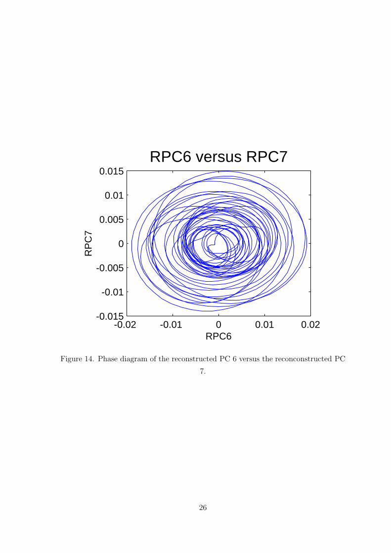
winter to early autumn 98. The same behaviour is also observed in the phase diagram

in the RPC 6 versus RPC 7 (Fig. 14).

Since EOF analysis does not focus on a particular frequency band, one would

expect MJO to project onto more than one PC. In fact, MJO is found to project onto

25

-0.02 -0.01 0 0.01 0.02-0.015

-0.01

-0.005

0

0.005

0.01

0.015

RPC6

RP

C7

RPC6 versus RPC7

Figure 14. Phase diagram of the reconstructed PC 6 versus the reconconstructed PC

7.

26

01/01/96 02/01/96 03/01/96 04/01/96 05/01/96

-0.01

-0.005

0

0.005

0.01

Time

RP

C1

to 8

Reconstructed PC1 to 8 from extended EOFs 8 & 9

RPC1RPC2RPC3RPC4RPC5RPC6RPC7RPC8

Figure 15. Reconstructed PCs 1 to 8 using the extended EOFs/PCs 8 and 9.

various PCs but with differing energies (amplitudes). For instance SSA analysis of

single PCs reveals that MJO is mostly present in higher PCs, e.g. PCs 6 and 7. This

observation is also revealed from analysing the reconstructed PC’s using the extended

EOFs/PCs 8 and 9 associated with the oscillation. This is well illustrated in figure

15, which shows the first 8 reconstructed PCs. Reconstructed PCs 5 to 8 are the most

energetic components representing MJO. Note in particular the weak projection of

MJO onto the first PC, which represents only the seasonal cycle.

The reconstructed or filtered PCs allow a reconstruction of the original space-time

OLR field. Figure 16 shows a hovmoller diagram of the reconstructed OLR field, at

10oN using the MJO-related extended EOFs/PCs 8 and 9. The reconstructed PC’s

1 to 8 (Fig. 15) are used in conjunction with the EOFs as in (11) to get the MJO

reconstructed field. It is clear from figure 16 that MJO gets triggered at around 25-

30oE over the African jet region. It reaches its mature stage over the Indian ocean in

the Bay of Bengal and starts to decay thereafter. The MJO gets particularly damped

near 150oE over the convective region in the warm pool. Figure 16 shows also the

dispersive nature of the MJO with a stronger phase speed during the growth phase

compared to that observed during the decay phase.

27

-24

-19

-14

-10

-5

0

5

10

14

19

24

0 50 100 150 200 250 300 35003/02/97

11/02/97

19/02/97

27/02/97

07/03/97

15/03/97

23/03/97

31/03/97

08/04/97

16/04/97

24/04/97

02/05/97

10/05/97

Longitude

Reconstructed OLR from extended EEOFs 8 & 9 at 5N (wm-2)

Figure 16. Reconstructed OLR field using the reconstructed EOFs/PCs 1 to 8

shown in Fig. 15.

28

6 Summary and conclusion

We have explained in this primer how to derive and compute EOFs for climate grid-

ded data. We pointed out particularly the meaning of EOFs and their physical in-

terpretability. We have also highlighted the major drawbacks of the method, namely

orthogonality of EOFs and uncorrelation of PCs. In addition, the truncation order

for signal/background noise separation remains arbitrary. We have illustrated the

method by applying it to the winter monthly SLP. We obtained in particular the

familiar Arctic Oscillation pattern as leading EOF and the Pacific pattern as second

EOF. The first EOF seems nondegenerate but the remainder of the spectrum looks

continuous.

Rotated EOFs are then presented as a way to overcome some of the previous

drawbacks related to orthogonality and uncorrelation. REOFs also help overcome the

problem of degenerate eigenspectrum. They attempt to maximise a simplicity criteria

by rotating a fixed number of EOFs. We have also illustrated the method with the

winter monthly SLP. The method yields the NAO as the leading REOF and the

Pacific pattern as second REOF. We have also highlighted the dependence of REOFs

on the number of retained EOFs and also the rotation criteria. For example, when

the number of retained EOFs increases the REOFs become more and more localised.

Extended EOFs (or MSSA) are presented as a way to overcome some of the short-

comings of EOFs, namely the use of only spatial correlation. MSSA makes use of

spatial as well as temporal correlation by extending the familiar state vector by in-

cluding explicitely the time information. The method can be used as a tool to filter

the data, isolate a trend, or even sparate an oscillatory component burried in the

noisy data. We have illustrated the approach with 5 years of daily OLR data. We

have in particular identified the seasonal cycle and the semi-annual oscillation. The

MJO was also identified from the spectrum of the extended data (or trajectory) ma-

trix. various characteristics of MJO have also been identified such as the most active

region of growth and decay phase, approximate period, and phase speed.

Acknowledgement.

This work was supported by the Centre for Global Atmospheric Modeling at the

Department of Meteorology, the University of Reading. I would like to thank par-

ticularly Prof J. Slingo for her interest in and encouragement of this work, Dr D. B.

Stephenson for his encouragement and his constructive critics. Particular thanks also

go to Dr C. Ferro for thouroughly reading the paper and providing positive comments,

and Prof I. Jolliffe for his constructive comments, Dr S. Pezzulli for his encouragement.

29

Thanks also to Dr P. Inness for providing the OLR data.

30

References

Angstrom, A., 1935: Geografiska Annaler, 17, 242-258.

Bjerknes, J., 1969: Atmospheric teleconnections from the equatorial Pa-

cific. Mon. Wea. Rev., 97, 163-172.

Broomhead, D. S., and G. P. King, 1986a: Extracting qualitative dynamics

from experimental data. Physica D, 20, 217-236.

Broomhead, D. S., and G. P. King, 1986b: On the qualitative analysis of

experimental dynamical systems. Nonlinear Phenomena and Chaos,

S. Sarkar, Ed., Adam Hilger, 113-144.

Caroll, J. B., 1953: An analytical solution for approximating simple struc-

ture in factor analysis. Psychometrika, 18, 23-38.

Craddock, J. M., 1973: Problems and prospects for eigenvector analysis

in meteorology. The statistician, 22, 133-145.

Dommenget, D., and M. Latif, 2002: A cautionary note on the interpre-

tation of EOFs. J. Climate, 15, 216-225.

Fraedrick, K., 1986: Estimating the dimensions of weather and climate

attractors. J. Atmos. Sci., 43, 419-432.

Fukuoka, A., 1951: A study of 10-day forecast (A synthetic report). The

Geophysical Magazine, Tokyo, Vol. XXII, 177-218.

Hendon, H. H., and M. L. Salby, 1994: The life cycle of the Madden-Julian

oscillation. J. Atmos. Sci., 51, 2225-2237.

Hotelling, H., 1933: Analysis of a complex of statistical variables into

principal components. J. Educ. Psych,, 24, 417-520.

Jolliffe, I. T., 2002: Principal Component Analysis. Springer-Verlag, 2nd

Edition, New York.

Kiladis, G. N., and K. M. Weickmann, 1992: Circulation anomalies as-

sociated with tropical convection during northern winter. Mon. Wea.

Rev., 120, 1900-1923.

Kimoto, M., M. Ghil, and K. C. Mo, 1991: Spatial structure of the extra-

tropical 40-day oscillation . Proc. 8’th Conf. Atmos. Oceanic waves

and Stability, Amer. Meteor. Soc., Boston, 115-116.

Knutson, T. R., and K. M. Weickmann, 1987: 30-60 day atmospheric oscil-

lations: composite life cycles of convection and circulation anomalies.

Mon. Wea. Rev., 115, 1407-1436.

Krishnamurthi, T. N., D. R., Chakraborty, N., Cubucku, L., Stefanova,

and T. S. V., Vijaya Kumar, 2003: A mechanism of the Madden-

Julian oscillation based on interactions in the frequency domain. Q. J.

31

R. Meteorol. Soc., 129, 2559-2590.

Kutzbach, J. E., 1967: Empirical eigenvectors of sea-level pressure, surface

temperature and precipitation complexes over North America. J. Appl.

Meteor., 6, 791-802.

Linz, P., and R. L. C. Wang, 2003: Exploring Numerical Methods: An In-

troduction to Scientific Computing Using MATLAB. Jones and Bartlett

Publishers, Sudbury, Massachusetts.

Loeve, M., 1978: Probability theory, Vol II, 4’th ed., Springer-Verlag, 413

pp.

Lorenz, E. N., 1970: Climate change as a mathematical problem. J. Appl.

Meteor., 9, 325-329.

Lorenz, E. N., 1956: Empirical orthogonal functions and statistical weather

prediction. Technical report, Statistical Forecast Project Report 1,

Dept. of Meteor., MIT, 1956. 49pp.

Madden, R. A., and P. R. Julian, 1971: Detection of a 40-50 day oscillation

in the zonal wind in the tropical pacific. J. Atmos. Sci., 28, 702-708.

Madden, R. A., and P. R. Julian, 1972: Description of global-scale circu-

lation cells in the tropics with a 40-50 day period. J. Atmos. Sci., 29,

1109-1123.

Madden, R. A., and P. R. Julian, 1994: Observations of the 40-50-day

tropical oscillation−A review. Mon. Wea. Rev, 122, 814-837.

Matthews, A. J., 2000: Propagation mechanisms for the Madden-Julian

oscillation. Q. J. R. Meteorol. Soc., 126, 2637-2651.

North, G. R., T. L., Bell, R. F. Cahalan, and F. J. Moeng, 1982: Sam-

pling errors in the estimation of empirical orthogonal functions. Mon.

Weather Rev., 110, 699-706.

Obukhov, A. M., 1960: The statistically orthogonal expansion of empirical

functions. Bull. Acad. Sci. USSR Geophys. Ser. (English Transl.),

288-291.

Obukhov, A.M., 1947: Statistically homogeneous fields on a sphere. Usp.

Mat. Navk., 2, 196-198.

Plaut, G., and R. Vautard, 1994: Spells of low-frequency oscillations and

weather regimes in the northern hemisphere. J. Atmos. sci., 51, 210-

236.

Richman, M. B., 1986: Rotation of principal components. J. Climatol.,

6, 293-335.

Simmons, A. J., G. W. Branstator, and J. M. Wallace, 1983: Barotropic

32

wave propagation, instability and atmospheric teleconnection paaterns.

J. Atmos. Sci., 40, 1363-1392.

von Storch, H., 1995: Spatial patterns: EOFs and CCA. In H. von Storch

and A. Navarra, editors, Analysis of Climate Variability: Application

of Statistical Techniques, Springer Verlag, 227-257.

von Storch, H., and F. W. Zwiers, 1999: Statistical Analysis in Climate

research, Cambridge University Press, Cambridge.

Thompson, D. W. J., and J. M. Wallace, 1998: The Arctic Oscillation

signature in wintertime signature in wintertime geopotential height

and temperature fields. Geophys. Res. Lett, 25, 1297-1300.

Thompson, D. W. J., and J. M. Wallace, 2000: Annular modes in the ex-

tratropical circulation. Part I: Month-to-month variability. J. Climate,

13, 1000-1016.

Thurstone, L. L., 1940: Current issues in factor analysis. Psychological

Bulletin, 37, 189-236.

Thurstone, L. L., 1947: Multiple Factor Analysis, The University of Chicago

Press, Chicago.

Vautard, R., P. Yiou, and M. Ghil, 1992: Singular spectrum analysis: A

toolkit for short, noisy chaotic signals. Physica D, 58, 95-126.

Wallace, J. M., and D. S. Gutzler, 1981: Teleconnections in the geopoten-

tial height field during the Northern Hemisphere winter. Mon. Weath.

Rev., 109, 784-812.

Weare, B. C., and J. S. Nasstrom, 1982: Examples of extended empirical

orthogonal function analysis. Mon. Weath. Rev., 110, 481-485.

Wilks, D. S., 1995: Statistical Methods in the Atmospheric Sciences. Aca-

demic Press, San Diego.

33