A Perspective on Computational Algorithms for Aerodynamic

Analysis and Design

Antony Jameson∗

Abstract

This paper examines the use of computational fluid dynamics as a tool for aircraft design. It addressesthe requirements for effective industrial use, and trade-offs between modeling accuracy and computationalcosts. Essential elements of algorithm design are discussed in detail, together with a unified approachto the design of shock capturing schemes. Finally, the paper discusses the use of techniques drawn fromcontrol theory to determine optimal aerodynamic shapes. In the future multidisciplinary analysis andoptimization should be combined to take account of the trade-offs in the overall performance of thecomplete system.

1 Introduction

Computational methods first began to have a significant impact on aerodynamics analysis and design inthe period of 1965-75. This decade saw the introduction of panel methods which could solve the linearflow models for arbitrarily complex geometry in both subsonic and supersonic flow [69, 167, 203]. It alsosaw the appearance of the first satisfactory methods for treating the nonlinear equations of transonic flow[137, 136, 76, 77, 51, 64], and the development of the hodograph method for the design of shock freesupercritical airfoils [19].

Algorithms have been the subject of intensive development for the past two decades. The principlesunderlying the design and implementation of robust schemes which can accurately resolve shock waves andcontact discontinuities in compressible flows are now quite well established. It is also quite well understoodhow to design high order schemes for viscous flow, including compact schemes and spectral methods. Adap-tive refinement of the mesh interval (h) and the order of approximations (p) has been successfully exploitedboth separately and in combination in the h-p method [140]. A continuing obstacle to the treatment ofconfigurations with complex geometry has been the problem of mesh generation. Several general techniqueshave been developed, including algebraic transformations and methods based on the solution of elliptic andhyperbolic equations. In the last few years methods using unstructured meshes have also begun to gainmore general acceptance. The Dassault-INRIA group led the way in developing a finite element method fortransonic potential flow. They obtained a solution for a complete Falcon 50 as early as 1982 [29]. Eulermethods for unstructured meshes have been the subject of intensive development by several groups since1985 [120, 92, 91, 186, 18], and Navier-Stokes methods on unstructured meshes have also been demonstrated[128, 129, 15].

Computational Fluid Dynamics (CFD) is now widely accepted as a key tool for aerodynamic design. Itseffectiveness is still hampered, however, by the long set-up and high costs, both human and computationalof complex flow simulations. The essential requirements for industrial use are:

1. assured accuracy

2. acceptable computational and human costs

3. fast turn around.∗Department of Aeronautics and Astronautics, Stanford University, Durand Buliding, Stanford, CA 94305-4035

1

2 THE COMPLEXITY OF FLUID FLOW AND MATHEMATICAL MODELING 2

Improvements are still needed in all three areas. In particular, the fidelity of modelling of high Reynoldsnumber viscous flows continues to be limited by computational costs. Consequently accurate and costeffective simulation of viscous flow at Reynolds numbers associated with full scale flight, such as the predictionof high lift devices, remains a challenge. Several routes are available toward the reduction of computationalcosts, including the reduction of mesh requirements by the use of higher order schemes, improved convergenceto a steady state by sophisticated acceleration methods, fast inversion methods for implicit schemes, and theexploitation of massively parallel computers.

Another factor limiting the effective use of CFD is the lack of good interfaces to computer aided design(CAD) systems. The geometry models provided by existing CAD systems often fail to meet the requirementsof continuity and smoothness needed for flow simulation, with the consequence that they must be modifiedbefore they can be used to provide the input for mesh generation. This bottleneck, which impedes theautomation of the mesh generation process, needs to be eliminated, and the CFD software should be fullyintegrated in a numerical design environment. In addition to more accurate and cost-effective flow predictionmethods, better optimizations methods are also needed, so that not only can designs be rapidly evaluated,but directions of improvement can be identified. Possession of techniques which result in a faster designcycle gives a crucial advantage in a competitive environment.

A critical issue, examined in the next section, is the choice of mathematical models. What level ofcomplexity is needed to provide sufficient accuracy for aerodynamic design, and what is the impact on costand turn-around time? Section 3 addresses the design of numerical algorithms for flow simulation. Section4 presents the results of some numerical calculations which require moderate computer resources and couldbe completed with the fast turn-around required by industrial users. Section 5 discusses automatic designprocedures which can be used to produce optimum aerodynamic designs. Finally, Section 6 offers an outlookfor the future.

2 The Complexity of Fluid Flow and Mathematical Modeling

2.1 The Hierarchy of Mathematical Models

Many critical phenomena of fluid flow, such as shock waves and turbulence, are essentially non-linear. Theyalso exhibit extreme disparities of scales. While the actual thickness of a shock wave is of the order of amean free path of the gas particles, on a macroscopic scale its thickness is essentially zero. In turbulentflow energy is transferred from large scale motions to progressively smaller eddies until the scale becomes sosmall that the motion is dissipated by viscosity. The ratio of the length scale of the global flow to that of thesmallest persisting eddies is of the order Re

34 , where Re is the Reynolds number, typically in the range of 30

million for an aircraft. In order to resolve such scales in all three space directions a computational grid withthe order of Re

94 cells would be required. This is beyond the range of any current or foreseeable computer.

Consequently mathematical models with varying degrees of simplification have to be introduced in order tomake computational simulation of flow feasible and produce viable and cost-effective methods.

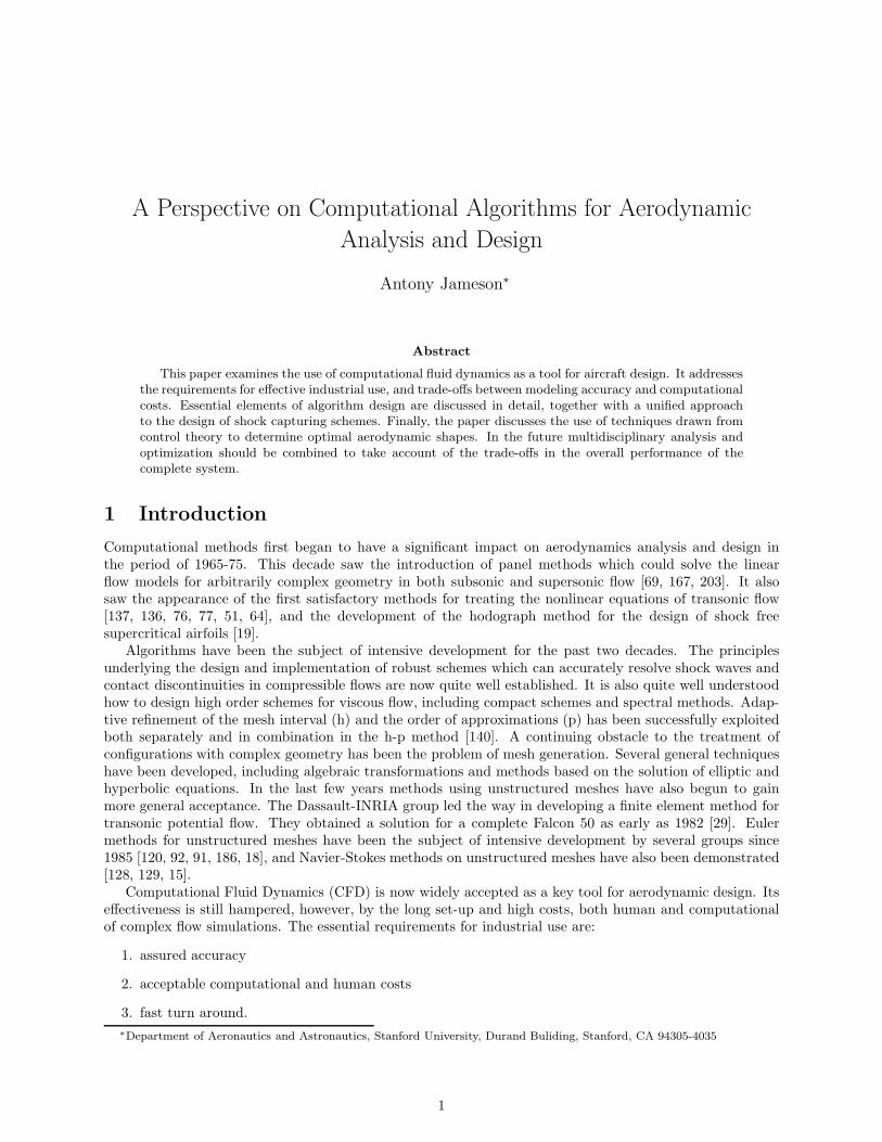
Figure 1 (supplied by Pradeep Raj) indicates a hierarchy of models at different levels of simplificationwhich have proved useful in practice. Efficient flight is generally achieved by the use of smooth and stream-lined shapes which avoid flow separation and minimize viscous effects, with the consequence that usefulpredictions can be made using inviscid models. Inviscid calculations with boundary layer corrections canprovide quite accurate predictions of lift and drag when the flow remains attached, but iteration between theinviscid outer solution and the inner boundary layer solution becomes increasingly difficult with the onsetof separation. Procedures for solving the full viscous equations are likely to be needed for the simulation ofarbitrary complex separated flows, which may occur at high angles of attack or with bluff bodies. In orderto treat flows at high Reynolds numbers, one is generally forced to estimate turbulent effects by Reynoldsaveraging of the fluctuating components. This requires the introduction of a turbulence model. As theavailable computing power increases one may also aspire to large eddy simulation (LES) in which the largerscale eddies are directly calculated, while the influence of turbulence at scales smaller than the mesh intervalis represented by a subgrid scale model.

2 THE COMPLEXITY OF FLUID FLOW AND MATHEMATICAL MODELING 3

Figure 1: Hierarchy of Fluid Flow Models

2.2 Computational Costs

Computational costs vary drastically with the choice of mathematical model. Panel methods can be effective-ly used to solve the linear potential flow equation with higher-end personal computers (with an Intel Pentiummicroprocessor, for example). Studies of the dependency of the result on mesh refinement, performed bythis author and others, have demonstrated that inviscid transonic potential flow or Euler solutions for anairfoil can be accurately calculated on a mesh with 160 cells around the section, and 32 cells normal to thesection. Using multigrid techniques 10 to 25 cycles are enough to obtain a converged result. Consequentlyairfoil calculations can be performed in seconds on a Cray YMP, and can also be performed on Pentium-classpersonal computers. Correspondingly accurate three-dimensional inviscid calculations can be performed fora wing on a mesh, say with 192×32×48 = 294, 912 cells, in about 5 minutes on a single processor CrayYMP, or less than a minute with eight processors, or in less than an hour on a workstation such as a SiliconGraphics Indigo 2.

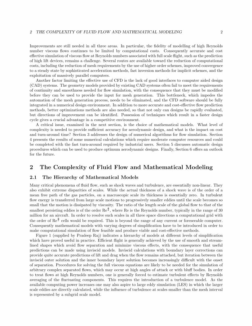
Viscous simulations at high Reynolds numbers require vastly greater resources. Careful two-dimensionalstudies of mesh requirements have been carried out at Princeton by Martinelli [124]. He found that on theorder of 32 mesh intervals were needed to resolve a turbulent boundary layer, in addition to 32 intervals be-tween the boundary layer and the far field, leading to a total of 64 intervals. In order to prevent degradationsin accuracy and convergence due to excessively large aspect ratios (in excess of 1,000) in the surface meshcells, the chordwise resolution must also be increased to 512 intervals. Reasonably accurate solutions can beobtained in a 512×64 mesh in 100 multigrid cycles. Translated to three dimensions, this would imply theneed for meshes with 5–10 million cells (for example, 512×64×256 = 8,388,608 cells as shown in Figure 2).When simulations are performed on less fine meshes with, say, 500,000 to 1 million cells, it is very hard toavoid mesh dependency in the solutions as well as sensitivity to the turbulence model.

A typical algorithm requires of the order of 5,000 floating point operations per mesh point in one multigriditeration. With 10 million mesh points, the operation count is of the order of 0.5×1011 per cycle. Givena computer capable of sustaining 1011 operations per second (100 gigaflops), 200 cycles could then beperformed in 100 seconds. Simulations of unsteady viscous flows (flutter, buffet) would be likely to require1,000–10,000 time steps. A further progression to large eddy simulation of complex configurations wouldrequire even greater resources. The following estimate is due to W.H. Jou [100]. Suppose that a conservativeestimate of the size of eddies in a boundary layer that ought to be resolved is 1/5 of the boundary layerthickness. Assuming that 10 points are needed to resolve a single eddy, the mesh interval should then be 1/50of the boundary layer thickness. Moreover, since the eddies are three-dimensional, the same mesh intervalshould be used in all three directions. Now, if the boundary layer thickness is of the order of 0.01 of thechord length, 5,000 intervals will be needed in the chordwise direction, and for a wing with an aspect ratioof 10, 50,000 intervals will be needed in the spanwise direction. Thus, of the order of 50× 5, 000× 50, 000or 12.5 billion mesh points would be needed in the boundary layer. If the time dependent behavior of theeddies is to be fully resolved using time steps on the order of the time for a wave to pass through a meshinterval, and one allows for a total time equal to the time required for waves to travel three times the lengthof the chord, of the order of 15,000 time steps would be needed. A more refined estimate which allows for

2 THE COMPLEXITY OF FLUID FLOW AND MATHEMATICAL MODELING 4

32 cells

32 cells in theboundary layer

512 cells around the wing to limitthe mesh aspect ratio (to about 1000)

256 cellsspanwise

Surface Mesh

Total: 512 x 64 x 256 = 8 388 608 cells

Figure 2: Mesh Requirements for a Viscous Simulation

the varying thickness of the boundary layer, recently made by Spalart et al. [182], suggests an even moresevere requirement. Performance beyond the teraflop (1012 operations per second) will be needed to attemptcalculations of this nature, which also have an information content far beyond what is needed for engineringanalysis and design. The designer does not need to know the details of the eddies in the boundary layer.The primary purpose of such calculations is to improve the calculation of averaged quantities such as skinfriction, and the prediction of global behavior such as the onset of separation. The main current use ofNavier-Stokes and large eddy simulations is to try to gain an improved insight into the physics of turbulentflow, which may in turn lead to the development of more comprehensive and reliable turbulence models.

2.3 Turbulence Modeling

It is doubtful whether a universally valid turbulence model, capable of describing all complex flows, couldbe devised [62]. Algebraic models [35, 13] have proved fairly satisfactory for the calculation of attachedand slightly separated wing flows. These models rely on the boundary layer concept, usually incorporatingseparate formulas for the inner and outer layers, and they require an estimate of a length scale which dependson the thickness of the boundary layer. The estimation of this quantity by a search for a maximum of thevorticity times a distance to the wall, as in the Baldwin-Lomax model, can lead to ambiguities in internalflows, and also in complex vortical flows over slender bodies and highly swept or delta wings [47, 125]. TheJohnson-King model [98], which allows for non-equilibrium effects through the introduction of an ordinarydifferential equation for the maximum shear stress, has improved the prediction of flows with shock inducedseparation [168, 101].

Closure models depending on the solution of transport equations are widely accepted for industrialapplications. These models eliminate the need to estimate a length scale by detecting the edge of theboundary layer. Eddy viscosity models typically use two equations for the turbulent kinetic energy k andthe dissipation rate ε, or a pair of equivalent quantities [99, 202, 183, 1, 133, 40]. Models of this type generallytend to present difficulties in the region very close to the wall. They also tend to be badly conditioned fornumerical solution. The k − l model [176] is designed to alleviate this problem by taking advantage of thelinear behaviour of the length scale l near the wall. In an alternative approach to the design of models whichare more amenable to numerical solution, new models requiring the solution of one transport equation haverecently been introduced [14, 181]. The performance of the algebraic models remains competitive for wing

3 CFD ALGORITHMS 5

flows, but the one- and two-equation models show promise for broader classes of flows. In order to achievegreater universality, research is also being pursued on more complex Reynolds stress transport models, whichrequire the solution of a larger number of transport equations.

Another direction of research is the attempt to devise more rational models via renormalization group(RNG) theory [206, 177]. Both algebraic and two-equation k−ε models devised by this approach have shownpromising results [126].

The selection of sufficiently accurate mathematical models and a judgment of their cost effectivenessultimately rests with industry. Aircraft and spacecraft designs normally pass through the three phases ofconceptual design, preliminary design, and detailed design. Correspondingly, the appropriate CFD modelswill vary in complexity. In the conceptual and preliminary design phases, the emphasis will be on relativelysimple models which can give results with very rapid turn-around and low computer costs, in order to evaluatealternative configurations and perform quick parametric studies. The detailed design stage requires the mostcomplete simulation that can be achieved with acceptable cost. In the past, the low level of confidence thatcould be placed on numerical predictions has forced the extensive use of wind tunnel testing at an early stageof the design. This practice was very expensive. The limited number of models that could be fabricated alsolimited the range of design variations that could be evaluated. It can be anticipated that in the future, therole of wind tunnel testing in the design process will be more one of verification. Experimental research toimprove our understanding of the physics of complex flows will continue, however, to play a vital role.

3 CFD Algorithms

3.1 Difficulties of Flow Simulation

The computational simulation of fluid flow presents a number of severe challenges for algorithm design. Atthe level of inviscid modeling, the inherent nonlinearity of the fluid flow equations leads to the formationof singularities such as shock waves and contact discontinuities. Moreover, the geometric configurations ofinterest are extremely complex, and generally contain sharp edges which lead to the shedding of vortexsheets. Extreme gradients near stagnation points or wing tips may also lead to numerical errors that canhave global influence. Numerically generated entropy may be convected from the leading edge for example,causing the formation of a numerically induced boundary layer which can lead to separation. The need totreat exterior domains of infinite extent is also a source of difficulty. Boundary conditions imposed at artificialouter boundaries may cause reflected waves which significantly interfere with the flow. When viscous effectsare also included in the simulation, the extreme difference of the scales in the viscous boundary layer andthe outer flow, which is essentially inviscid, is another source of difficulty, forcing the use of meshes withextreme variations in mesh interval. For these reasons CFD, has been a driving force for the developmentof numerical algorithms.

3.2 Structured and Unstructured Meshes

The algorithm designer faces a number of critical decisions. The first choice that must be made is the natureof the mesh used to divide the flow field into discrete subdomains. The discretization procedure must allowfor the treatment of complex configurations. The principal alternatives are Cartesian meshes, body-fittedcurvilinear meshes, and unstructured tetrahedral meshes. Each of these approaches has advantages whichhave led to their use. The Cartesian mesh minimizes the complexity of the algorithm at interior pointsand facilitates the use of high order discretization procedures, at the expense of greater complexity, andpossibly a loss of accuracy, in the treatment of boundary conditions at curved surfaces. This difficulty maybe alleviated by using mesh refinement procedures near the surface. With their aid, schemes which useCartesian meshes have recently been developed to treat very complex configurations [132, 169, 26, 105].

Body-fitted meshes have been widely used and are particularly well suited to the treatment of viscousflow because they readily allow the mesh to be compressed near the body surface. With this approach, theproblem of mesh generation itself has proved to be a major pacing item. The most commonly used proceduresare algebraic transformations [11, 52, 55, 178], methods based on the solution of elliptic equations, pioneeredby Thompson [192, 193, 179, 180], and methods based on the solution of hyperbolic equations marching out

3 CFD ALGORITHMS 6

from the body [184]. In order to treat very complex configurations it generally proves expedient to use amultiblock [201, 170] procedure, with separately generated meshes in each block, which may then be patchedat block faces, or allowed to overlap, as in the Chimera scheme [23, 24]. While a number of interactivesoftware systems for grid generation have been developed, such as EAGLE, GRIDGEN, and ICEM, thegeneration of a satisfactory grid for a very complex configuration may require months of effort.

The alternative is to use an unstructured mesh in which the domain is subdivided into tetrahedra.This in turn requires the development of solution algorithms capable of yielding the required accuracy onunstructured meshes. This approach has been gaining acceptance, as it is becoming apparent that it can leadto a speed-up and reduction in the cost of mesh generation that more than offsets the increased complexityand cost of the flow simulations. Two competing procedures for generating triangulations which have bothproved successful are Delaunay triangulation [48, 15], based on concepts introduced at the beginning of thecentury by Voronoi [199], and the moving front method [121].

3.3 Finite Difference, Finite Volume, and Finite Element Schemes

Associated with choice of mesh type is the formulation of the discretization procedure for the equations offluid flow, which can be expressed as differential conservation laws. In the Cartesian tensor notation, let xi

be the coordinates, p, ρ, T , and E the pressure, density, temperature, and total energy, and ui the velocitycomponents. Using the convention that summation over j = 1, 2, 3 is implied by a repeated subscript j, eachconservation equation has the form

∂w

∂t+

∂fj∂xj

− ∂fvj

∂xj= 0. (1)

where fj are the inviscid (convective) fluxes, and fvj are the viscous fluxes. For the mass equation

w = ρ, fj = ρuj.

For the i momentum equation

wi = ρui, fij = ρuiuj + pδij , fvij = σij ,

where σij is the viscous stress tensor. For the energy equation

w = ρE, fj = pHuj, fvj = σjkuk − k∂T

∂xj,

where k is the coefficient of thermal conductivity. The pressure is related to the density and energy by theequation of state

p = (γ − 1)ρ(E − 1

2uiui

)(2)

in which γ is the ratio of specific heats and the stagnation enthalpy is given by

H = E +p

ρ

whileE = cvT +

12uiui

where cv is the specific heat at constant volume. In the Navier-Stokes equations the viscous stresses areassumed to be linearly proportional to the rate of strain, or

σij = µ

(∂ui

∂xj+

∂uj

∂xi

)+ λδij

(∂uk

∂xk

), (3)

where µ and λ are the coefficients of viscosity and bulk viscosity, and usually λ = −2µ/3. The coefficient ofthermal conductivity and temperature are given by the relations

k =cpµ

Pr, T =

p

Rρ

3 CFD ALGORITHMS 7

where cp is the specific heat at constant pressure, R is the gas constant, and Pr is the Prandtl number.The finite difference method, which requires the use of a Cartesian or a structured curvilinear mesh,

directly approximates the differential operators appearing in these equations. In the finite volume method[122], the discretization is accomplished by dividing the domain of the flow into a large number of smallsubdomains, and applying the conservation laws in the integral form

∂

∂t

∫Ω

wdV +∫∂Ω

f · dS = 0.

Here F is the flux appearing in equation (1) and dS is the directed surface element of the boundary ∂Ω ofthe domain Ω. The use of the integral form has the advantage that no assumption of the differentiabilityof the solutions is implied, with the result that it remains a valid statement for a subdomain containing ashock wave. In general the subdomains could be arbitrary, but it is convenient to use either hexahedral cellsin a body conforming curvilinear mesh or tetrahedrons in an unstructured mesh.

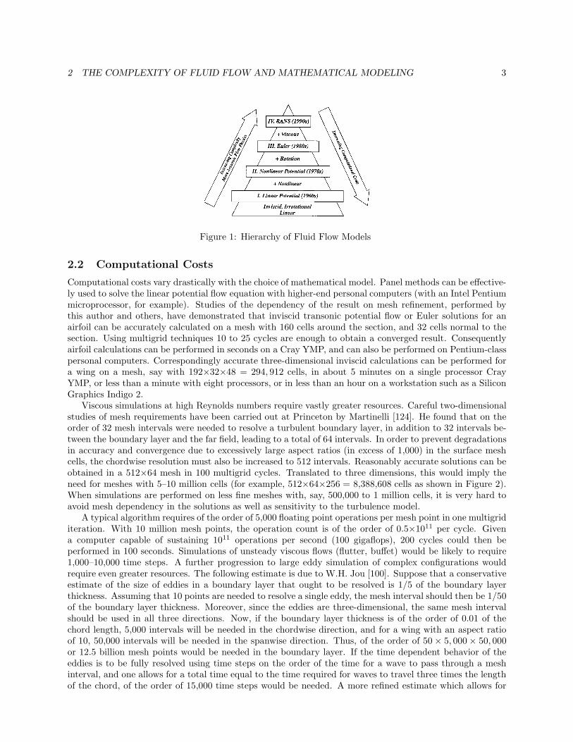
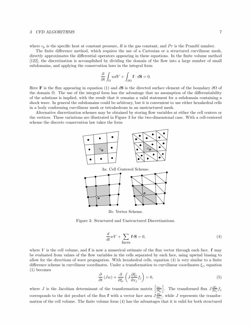
Alternative discretization schemes may be obtained by storing flow variables at either the cell centers orthe vertices. These variations are illustrated in Figure 3 for the two-dimensional case. With a cell-centeredscheme the discrete conservation law takes the form

o o

3a: Cell Centered Scheme.

o o

3b: Vertex Scheme.

Figure 3: Structured and Unstructured Discretizations.

d

dtwV +

∑faces

f ·S = 0, (4)

where V is the cell volume, and f is now a numerical estimate of the flux vector through each face. f maybe evaluated from values of the flow variables in the cells separated by each face, using upwind biasing toallow for the directions of wave propagation. With hexahedral cells, equation (4) is very similar to a finitedifference scheme in curvilinear coordinates. Under a transformation to curvilinear coordinates ξj , equation(1) becomes

∂

∂t(Jw) +

∂

∂ξi

(J

∂ξi∂xj

fj

)= 0, (5)

where J is the Jacobian determinant of the transformation matrix[∂xi

∂ξj

]. The transformed flux J ∂ξi

∂xjfj

corresponds to the dot product of the flux f with a vector face area J ∂ξi

∂xj, while J represents the transfor-

mation of the cell volume. The finite volume form (4) has the advantages that it is valid for both structured

3 CFD ALGORITHMS 8

and unstructured meshes, and that it assures that a uniform flow exactly satisfies the equations, because∑faces S = 0 for a closed control volume. Finite difference schemes do not necessarily satisfy this constraint

because of the discretization errors in evaluating ∂ξi

∂xjand the inversion of the transformation matrix. A

cell-vertex finite volume scheme can be derived by taking the union of the cells surrounding a given vertexas the control volume for that vertex [65, 82, 158]. In equation (4), V is now the sum of the volumes of thesurrounding cells, while the flux balance is evaluated over the outer faces of the polyhedral control volume.In the absence of upwind biasing the flux vector is evaluated by averaging over the corners of each face. Thishas the advantage of remaining accurate on an irregular or unstructured mesh. An alternative route to thediscrete equations is provided by the finite element method. Whereas the finite difference and finite volumemethods approximate the differential and integral operators, the finite element method proceeds by insertingan approximate solution into the exact equations. On multiplying by a test function φ and integrating byparts over space, one obtains the weak form

∂

∂t

∫ ∫ ∫Ω

φwdΩ =

∫ ∫ ∫Ω

f ·∇φdΩ−∫ ∫

∂Ω

φf ·dS (6)

which is also valid in the presence of discontinuities in the flow. In the Galerkin method the approximatesolution is expanded in terms of the same family of functions as those from which the test functions aredrawn. By choosing test functions with local support, separate equations are obtained for each node. Forexample, if a tetrahedral mesh is used, and φ is piecewise linear, with a nonzero value only at a single node,the equations at each node have a stencil which contains only the nearest neighbors. In this case the finiteelement approximation corresponds closely to a finite volume scheme. If a piecewise linear approximationto the flux f is used in the evaluation of the integrals on the right hand side of equation (6), these integralsreduce to formulas which are identical to the flux balance of the finite volume scheme.

Thus the finite difference and finite volume methods lead to essentially similar schemes on structuredmeshes, while the finite volume method is essentially equivalent to a finite element method with linearelements when a tetrahedral mesh is used. Provided that the flow equations are expressed in the conservationlaw form (1), all three methods lead to an exact cancellation of the fluxes through interior cell boundaries, sothat the conservative property of the equations is preserved. The important role of this property in ensuringcorrect shock jump conditions was pointed out by Lax and Wendroff [108].

3.4 Non-oscillatory Shock Capturing Schemes

3.4.1 Local Extremum Diminishing (LED) Schemes

The discretization procedures which have been described in the last section lead to nondissipative approxi-mations to the Euler equations. Dissipative terms may be needed for two reasons. The first is the possibilityof undamped oscillatory modes. The second reason is the need for the clean capture of shock waves andcontact discontinuities without undesirable oscillations. An extreme overshoot could result in a negativevalue of an inherently positive quantity such as the pressure or density. The next sections summarize aunified approach to the construction of nonoscillatory schemes via the introduction of controlled diffusiveand antidiffusive terms. This is the line adhered to in the author’s own work.

The development of non-oscillatory schemes has been a prime focus of algorithm research for compressibleflow. Consider a general semi-discrete scheme of the form

d

dtvj =

∑k =j

cjk(vk − vj). (7)

A maximum cannot increase and a minimum cannot decrease if the coefficients cjk are non-negative, sinceat a maximum vk − vj ≤ 0, and at a minimum vk − vj ≥ 0. Thus the condition

cjk ≥ 0, k = j (8)

is sufficient to ensure stability in the maximum norm. Moreover, if the scheme has a compact stencil, so thatcjk = 0 when j and k are not nearest neighbors, a local maximum cannot increase and local minimum cannot

3 CFD ALGORITHMS 9

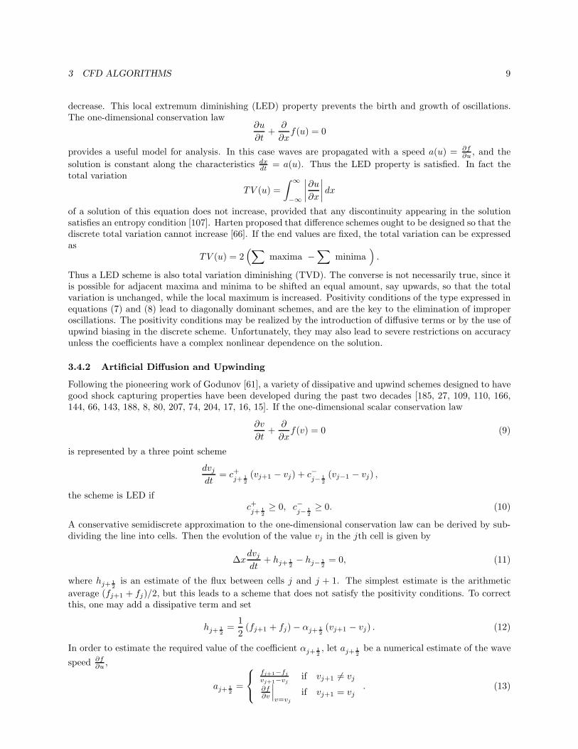
decrease. This local extremum diminishing (LED) property prevents the birth and growth of oscillations.The one-dimensional conservation law

∂u

∂t+

∂

∂xf(u) = 0

provides a useful model for analysis. In this case waves are propagated with a speed a(u) = ∂f∂u , and the

solution is constant along the characteristics dxdt = a(u). Thus the LED property is satisfied. In fact the

total variation

TV (u) =∫ ∞

−∞

∣∣∣∣∂u∂x∣∣∣∣ dx

of a solution of this equation does not increase, provided that any discontinuity appearing in the solutionsatisfies an entropy condition [107]. Harten proposed that difference schemes ought to be designed so that thediscrete total variation cannot increase [66]. If the end values are fixed, the total variation can be expressedas

TV (u) = 2(∑

maxima −∑

minima).

Thus a LED scheme is also total variation diminishing (TVD). The converse is not necessarily true, since itis possible for adjacent maxima and minima to be shifted an equal amount, say upwards, so that the totalvariation is unchanged, while the local maximum is increased. Positivity conditions of the type expressed inequations (7) and (8) lead to diagonally dominant schemes, and are the key to the elimination of improperoscillations. The positivity conditions may be realized by the introduction of diffusive terms or by the use ofupwind biasing in the discrete scheme. Unfortunately, they may also lead to severe restrictions on accuracyunless the coefficients have a complex nonlinear dependence on the solution.

3.4.2 Artificial Diffusion and Upwinding

Following the pioneering work of Godunov [61], a variety of dissipative and upwind schemes designed to havegood shock capturing properties have been developed during the past two decades [185, 27, 109, 110, 166,144, 66, 143, 188, 8, 80, 207, 74, 204, 17, 16, 15]. If the one-dimensional scalar conservation law

∂v

∂t+

∂

∂xf(v) = 0 (9)

is represented by a three point scheme

dvjdt

= c+j+ 1

2(vj+1 − vj) + c−

j− 12(vj−1 − vj) ,

the scheme is LED ifc+j+ 1

2≥ 0, c−

j− 12≥ 0. (10)

A conservative semidiscrete approximation to the one-dimensional conservation law can be derived by sub-dividing the line into cells. Then the evolution of the value vj in the jth cell is given by

∆xdvjdt

+ hj+ 12− hj− 1

2= 0, (11)

where hj+ 12is an estimate of the flux between cells j and j + 1. The simplest estimate is the arithmetic

average (fj+1 + fj)/2, but this leads to a scheme that does not satisfy the positivity conditions. To correctthis, one may add a dissipative term and set

hj+ 12=

12(fj+1 + fj)− αj+ 1

2(vj+1 − vj) . (12)

In order to estimate the required value of the coefficient αj+ 12, let aj+ 1

2be a numerical estimate of the wave

speed ∂f∂u ,

aj+ 12=

fj+1−fj

vj+1−vjif vj+1 = vj

∂f∂v

∣∣∣v=vj

if vj+1 = vj. (13)

3 CFD ALGORITHMS 10

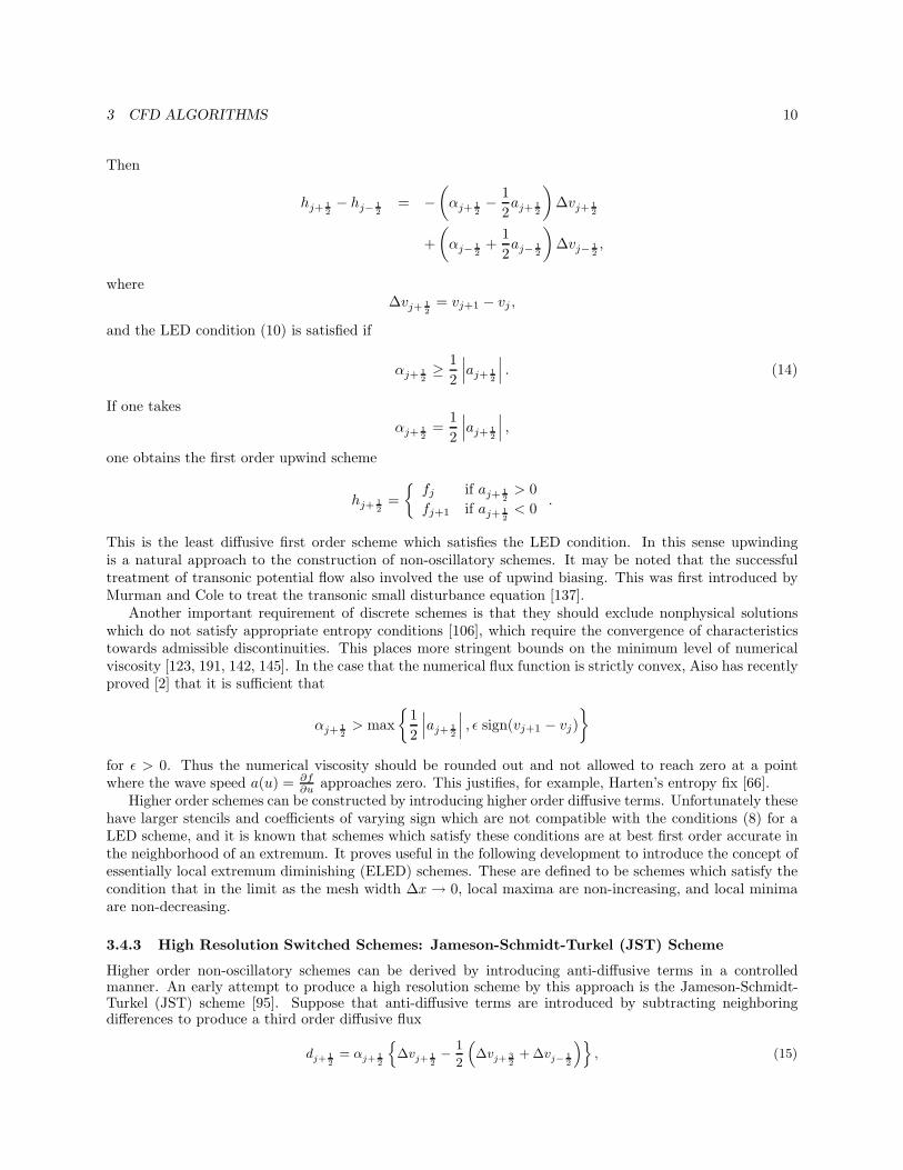
Then

hj+ 12− hj− 1

2= −

(αj+ 1

2− 1

2aj+ 1

2

)∆vj+ 1

2

+(αj− 1

2+

12aj− 1

2

)∆vj− 1

2,

where∆vj+ 1

2= vj+1 − vj ,

and the LED condition (10) is satisfied if

αj+ 12≥ 1

2

∣∣∣aj+ 12

∣∣∣ . (14)

If one takesαj+ 1

2=

12

∣∣∣aj+ 12

∣∣∣ ,one obtains the first order upwind scheme

hj+ 12=

fj if aj+ 12> 0

fj+1 if aj+ 12< 0 .

This is the least diffusive first order scheme which satisfies the LED condition. In this sense upwindingis a natural approach to the construction of non-oscillatory schemes. It may be noted that the successfultreatment of transonic potential flow also involved the use of upwind biasing. This was first introduced byMurman and Cole to treat the transonic small disturbance equation [137].

Another important requirement of discrete schemes is that they should exclude nonphysical solutionswhich do not satisfy appropriate entropy conditions [106], which require the convergence of characteristicstowards admissible discontinuities. This places more stringent bounds on the minimum level of numericalviscosity [123, 191, 142, 145]. In the case that the numerical flux function is strictly convex, Aiso has recentlyproved [2] that it is sufficient that

αj+ 12> max

12

∣∣∣aj+ 12

∣∣∣ , ε sign(vj+1 − vj)

for ε > 0. Thus the numerical viscosity should be rounded out and not allowed to reach zero at a pointwhere the wave speed a(u) = ∂f

∂u approaches zero. This justifies, for example, Harten’s entropy fix [66].Higher order schemes can be constructed by introducing higher order diffusive terms. Unfortunately these

have larger stencils and coefficients of varying sign which are not compatible with the conditions (8) for aLED scheme, and it is known that schemes which satisfy these conditions are at best first order accurate inthe neighborhood of an extremum. It proves useful in the following development to introduce the concept ofessentially local extremum diminishing (ELED) schemes. These are defined to be schemes which satisfy thecondition that in the limit as the mesh width ∆x → 0, local maxima are non-increasing, and local minimaare non-decreasing.

3.4.3 High Resolution Switched Schemes: Jameson-Schmidt-Turkel (JST) Scheme

Higher order non-oscillatory schemes can be derived by introducing anti-diffusive terms in a controlledmanner. An early attempt to produce a high resolution scheme by this approach is the Jameson-Schmidt-Turkel (JST) scheme [95]. Suppose that anti-diffusive terms are introduced by subtracting neighboringdifferences to produce a third order diffusive flux

dj+ 12= αj+ 1

2

∆vj+ 1

2− 1

2

(∆vj+ 3

2+∆vj− 1

2

), (15)

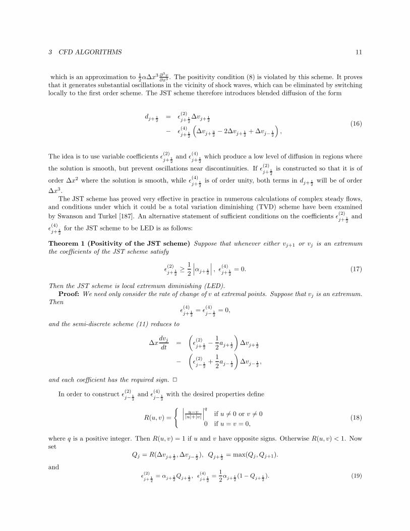
3 CFD ALGORITHMS 11

which is an approximation to 12α∆x3 ∂3v

∂x3 . The positivity condition (8) is violated by this scheme. It provesthat it generates substantial oscillations in the vicinity of shock waves, which can be eliminated by switchinglocally to the first order scheme. The JST scheme therefore introduces blended diffusion of the form

dj+ 12

= ε(2)

j+ 12∆vj+ 1

2

− ε(4)

j+ 12

(∆vj+ 3

2− 2∆vj+ 1

2+∆vj− 1

2

),

(16)

The idea is to use variable coefficients ε(2)

j+ 12and ε

(4)

j+ 12which produce a low level of diffusion in regions where

the solution is smooth, but prevent oscillations near discontinuities. If ε(2)

j+ 12is constructed so that it is of

order ∆x2 where the solution is smooth, while ε(4)

j+ 12is of order unity, both terms in dj+ 1

2will be of order

∆x3.The JST scheme has proved very effective in practice in numerous calculations of complex steady flows,

and conditions under which it could be a total variation diminishing (TVD) scheme have been examinedby Swanson and Turkel [187]. An alternative statement of sufficient conditions on the coefficients ε

(2)

j+ 12and

ε(4)

j+ 12for the JST scheme to be LED is as follows:

Theorem 1 (Positivity of the JST scheme) Suppose that whenever either vj+1 or vj is an extremumthe coefficients of the JST scheme satisfy

ε(2)

j+ 12≥ 1

2

∣∣∣αj+ 12

∣∣∣ , ε(4)

j+ 12= 0. (17)

Then the JST scheme is local extremum diminishing (LED).Proof: We need only consider the rate of change of v at extremal points. Suppose that vj is an extremum.

Thenε(4)

j+ 12= ε

(4)

j− 12= 0,

and the semi-discrete scheme (11) reduces to

∆xdvjdt

=(ε(2)

j+ 12− 1

2aj+ 1

2

)∆vj+ 1

2

−(ε(2)

j− 12+

12aj− 1

2

)∆vj− 1

2,

and each coefficient has the required sign.

In order to construct ε(2)

j− 12and ε

(4)

j− 12with the desired properties define

R(u, v) =

∣∣∣ u−v|u|+|v|

∣∣∣q if u = 0 or v = 00 if u = v = 0,

(18)

where q is a positive integer. Then R(u, v) = 1 if u and v have opposite signs. Otherwise R(u, v) < 1. Nowset

Qj = R(∆vj+ 12,∆vj− 1

2), Qj+ 1

2= max(Qj , Qj+1).

andε(2)

j+ 12= αj+ 1

2Qj+ 1

2, ε

(4)

j+ 12=

1

2αj+ 1

2(1−Qj+ 1

2). (19)

3 CFD ALGORITHMS 12

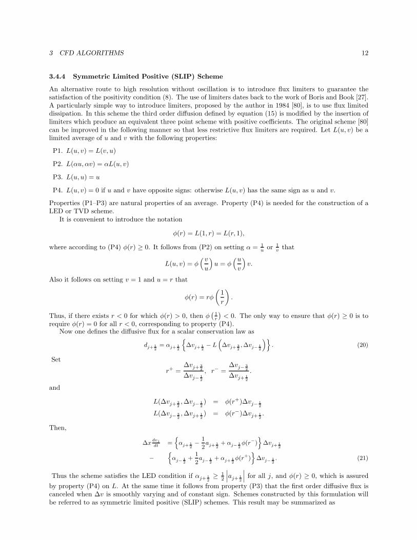
3.4.4 Symmetric Limited Positive (SLIP) Scheme

An alternative route to high resolution without oscillation is to introduce flux limiters to guarantee thesatisfaction of the positivity condition (8). The use of limiters dates back to the work of Boris and Book [27].A particularly simple way to introduce limiters, proposed by the author in 1984 [80], is to use flux limiteddissipation. In this scheme the third order diffusion defined by equation (15) is modified by the insertion oflimiters which produce an equivalent three point scheme with positive coefficients. The original scheme [80]can be improved in the following manner so that less restrictive flux limiters are required. Let L(u, v) be alimited average of u and v with the following properties:

P1. L(u, v) = L(v, u)

P2. L(αu, αv) = αL(u, v)

P3. L(u, u) = u

P4. L(u, v) = 0 if u and v have opposite signs: otherwise L(u, v) has the same sign as u and v.

Properties (P1–P3) are natural properties of an average. Property (P4) is needed for the construction of aLED or TVD scheme.

It is convenient to introduce the notation

φ(r) = L(1, r) = L(r, 1),

where according to (P4) φ(r) ≥ 0. It follows from (P2) on setting α = 1u or 1

v that

L(u, v) = φ( v

u

)u = φ

(u

v

)v.

Also it follows on setting v = 1 and u = r that

φ(r) = rφ

(1r

).

Thus, if there exists r < 0 for which φ(r) > 0, then φ(

1r

)< 0. The only way to ensure that φ(r) ≥ 0 is to

require φ(r) = 0 for all r < 0, corresponding to property (P4).Now one defines the diffusive flux for a scalar conservation law as

dj+ 12= αj+ 1

2

∆vj+ 1

2− L

(∆vj+ 3

2,∆vj− 1

2

). (20)

Set

r+ =∆vj+ 3

2

∆vj− 12

, r− =∆vj− 3

2

∆vj+ 12

.

and

L(∆vj+ 32,∆vj− 1

2) = φ(r+)∆vj− 1

2

L(∆vj− 32,∆vj+ 1

2) = φ(r−)∆vj+ 1

2.

Then,

∆xdvj

dt=αj+ 1

2− 1

2aj+ 1

2+ αj− 1

2φ(r−)

∆vj+ 1

2

−αj− 1

2+

1

2aj− 1

2+ αj+ 1

2φ(r+)

∆vj− 1

2. (21)

Thus the scheme satisfies the LED condition if αj+ 12≥ 1

2

∣∣∣aj+ 12

∣∣∣ for all j, and φ(r) ≥ 0, which is assuredby property (P4) on L. At the same time it follows from property (P3) that the first order diffusive flux iscanceled when ∆v is smoothly varying and of constant sign. Schemes constructed by this formulation willbe referred to as symmetric limited positive (SLIP) schemes. This result may be summarized as

3 CFD ALGORITHMS 13

Theorem 2 (Positivity of the SLIP scheme) Suppose that the discrete conservation law (11) containsa limited diffusive flux as defined by equation (20). Then the positivity condition (14), together with theproperties (P1–P4) for limited averages, are sufficient to ensure satisfaction of the LED principle that a localmaximum cannot increase and a local minimum cannot decrease.

A variety of limiters may be defined which meet the requirements of properties (P1–P4). Define

S(u, v) =12sign(u) + sign(v)

which vanishes is u and v have opposite signs.Then two limiters which are appropriate are the following well-known schemes:

1. Minmod:L(u, v) = S(u, v)min(|u|, |v|)

2. Van Leer:

L(u, v) = S(u, v)2|u||v||u|+ |v| .

In order to produce a family of limiters which contains these as special cases it is convenient to set

L(u, v) =12D(u, v)(u+ v),

where D(u, v) is a factor which should deflate the arithmetic average, and become zero if u and v haveopposite signs. Take

D(u, v) = 1−R(u, v) = 1−∣∣∣∣ u− v

|u|+ |v|∣∣∣∣q

, (22)

where R(u, v) is the same function that was introduced in the JST scheme, and q is a positive integer. ThenD(u, v) = 0 if u and v have opposite signs. Also if q = 1, L(u, v) reduces to minmod, while if q = 2, L(u, v)is equivalent to Van Leer’s limiter. By increasing q one can generate a sequence of limited averages whichapproach a limit defined by the arithmetic mean truncated to zero when u and v have opposite signs.

When the terms are regrouped, it can be seen that with this limiter the SLIP scheme is exactly equivalentto the JST scheme, with the switch is defined as

Qj+ 12

= R(∆vj+ 3

2,∆vj+ 1

2

)ε(2)

j+ 12

= αj+ 12Qj+ 1

2

ε(4)

j+ 12

= αj+ 12

(1−Qj+ 1

2

).

This formulation thus unifies the JST and SLIP schemes. The SLIP construction, however, provides aconvenient framework for the construction of LED schemes on unstructured meshes [87]

3.4.5 Essentially Local Extremum Diminishing (ELED) Scheme with Soft Limiter

The limiters defined by the formula (22) have the disadvantage that they are active at a smooth extrema,reducing the local accuracy of the scheme to first order. In order to prevent this, the SLIP scheme can berelaxed to give an essentially local extremum diminishing (ELED) scheme which is second order accurate atsmooth extrema by the introduction of a threshold in the limited average. Therefore redefine D(u, v) as

D(u, v) = 1−∣∣∣∣ u− v

max(|u|+ |v| , ε∆xr)

∣∣∣∣q

, (23)

where r = 32 , q ≥ 2. This reduces to the previous definition if |u|+ |v| > ε∆xr.

3 CFD ALGORITHMS 14

In any region where the solution is smooth, ∆vj+ 32−∆vj− 1

2is of order ∆x2. In fact if there is a smooth

extremum in the neighborhood of vj or vj+1, a Taylor series expansion indicates that ∆vj+ 32, ∆vj+ 1

2and

∆vj− 12are each individually of order ∆x2, since dv

dx = 0 at the extremum. It may be verified that secondorder accuracy is preserved at a smooth extremum if q ≥ 2. On the other hand the limiter acts in the usualway if

∣∣∣∆vj+ 32

∣∣∣ or ∣∣∣∆vj− 32

∣∣∣ > ε∆xr , and it may also be verified that in the limit ∆x → 0 local maximaare non increasing and local minima are non decreasing [87]. Thus the scheme is essentially local extremumdiminishing (ELED).

The effect of the “soft limiter” is not only to improve the accuracy: the introduction of a thresholdbelow which extrema of small amplitude are accepted also usually results in a faster rate of convergence toa steady state, and decreases the likelyhood of limit cycles in which the limiter interacts unfavorably withthe corrections produced by the updating scheme. In a scheme recently proposed by Venkatakrishnan athreshold is introduced precisely for this purpose [196].

3.4.6 Upstream Limited Positive (USLIP) Schemes

By adding the anti-diffusive correction purely from the upstream side one may derive a family of upstreamlimited positive (USLIP) schemes. Corresponding to the original SLIP scheme defined by equation (20), aUSLIP scheme is obtained by setting

dj+ 12= αj+ 1

2

∆vj+ 1

2− L

(∆vj+ 1

2,∆vj− 1

2

)if aj+ 1

2> 0, or

dj+ 12= αj+ 1

2

∆vj+ 1

2− L

(∆vj+ 1

2,∆vj+ 3

2

)if aj+ 1

2< 0. If αj+ 1

2= 1

2

∣∣∣aj+ 12

∣∣∣ one recovers a standard high resolution upwind scheme in semi-discreteform. Consider the case that aj+ 1

2> 0 and aj− 1

2> 0. If one sets

r+ =∆vj+ 1

2

∆vj− 12

, r− =∆vj− 3

2

∆vj− 12

,

the scheme reduces to∆x

dvj

dt= −1

2

φ(r+)aj+ 1

2+(2− φ(r−)

)aj− 1

2

∆vj− 1

2.

To assure the correct sign to satisfy the LED criterion the flux limiter must now satisfy the additionalconstraint that φ(r) ≤ 2.

The USLIP formulation is essentially equivalent to standard upwind schemes [144, 188]. Both the SLIPand USLIP constructions can be implemented on unstructured meshes [86, 87]. The anti-diffusive terms arethen calculated by taking the scalar product of the vectors defining an edge with the gradient in the adjacentupstream and downstream cells.

3.4.7 Systems of Conservation Laws: Flux Splitting and Flux-Difference Splitting

Steger and Warming [185] first showed how to generalize the concept of upwinding to the system of conser-vation laws

∂w

∂t+

∂

∂xf(w) = 0 (24)

by the concept of flux splitting. Suppose that the flux is split as f = f+ + f− where ∂f+

∂w and ∂f−

∂w havepositive and negative eigenvalues. Then the first order upwind scheme is produced by taking the numericalflux to be

hj+ 12= f+

j + f−j+1.

3 CFD ALGORITHMS 15

This can be expressed in viscosity form as

hj+ 12

=12(f+j+1 + f+

j

)− 12(f+j+1 − f+

j

)+12(f−j+1 + f−

j

)+

12(f−j+1 − f−

j

)=

12(fj+1 + fj)− dj+ 1

2,

where the diffusive flux isdj+ 1

2=

12∆(f+ − f−)j+ 1

2. (25)

Roe derived the alternative formulation of flux difference splitting [166] by distributing the corrections dueto the flux difference in each interval upwind and downwind to obtain

∆xdwj

dt+ (fj+1 − fj)− + (fj − fj−1)+ = 0,

where now the flux difference fj+1 − fj is split. The corresponding diffusive flux is

dj+ 12=

12

(∆f+

j+ 12−∆f−

j+ 12

).

Following Roe’s derivation, let Aj+ 12be a mean value Jacobian matrix exactly satisfying the condition

fj+1 − fj = Aj+ 12(wj+1 − wj). (26)

Aj+ 12may be calculated by substituting the weighted averages

u =

√ρj+1uj+1 +

√ρjuj√

ρj+1 +√ρj

,H =

√ρj+1Hj+1 +

√ρjHj√

ρj+1 +√ρj

(27)

into the standard formulas for the Jacobian matrix A = ∂f∂w . A splitting according to characteristic fields is

now obtained by decomposing Aj+ 12as

Aj+ 12= TΛT−1, (28)

where the columns of T are the eigenvectors of Aj+ 12, and Λ is a diagonal matrix of the eigenvalues. Now

the corresponding diffusive flux is12

∣∣∣Aj+ 12

∣∣∣ (wj+1 − wj),

where ∣∣∣Aj+ 12

∣∣∣ = T |Λ|T−1

and |Λ| is the diagonal matrix containing the absolute values of the eigenvalues.

3.4.8 Alternative Splittings

Characteristic splitting has the advantages that it introduces the minimum amount of diffusion to excludethe growth of local extrema of the characteristic variables, and that with the Roe linearization it allowsa discrete shock structure with a single interior point. To reduce the computational complexity one mayreplace |A| by αI where if α is at least equal to the spectral radius max |λ(A)|, then the positivity conditionswill still be satisfied. Then the first order scheme simply has the scalar diffusive flux

dj+ 12=

12αj+ 1

2∆wj+ 1

2. (29)

The JST scheme with scalar diffusive flux captures shock waves with about 3 interior points, and it has beenwidely used for transonic flow calculations because it is both robust and computationally inexpensive.

3 CFD ALGORITHMS 16

An intermediate class of schemes can be formulated by defining the first order diffusive flux as a combi-nation of differences of the state and flux vectors

dj+ 12=

1

2α∗

j+ 12c (wj+1 − wj) +

1

2βj+ 1

2(fj+1 − fj) , (30)

where the factor c is included in the first term to make α∗j+ 1

2and βj+ 1

2dimensionless. Schemes of this class

are fully upwind in supersonic flow if one takes α∗j+ 1

2= 0 and βj+ 1

2= sign(M) when the absolute value of

the Mach number M exceeds 1. The flux vector f can be decomposed as

f = uw + fp, (31)

where

fp =

0

pup

. (32)

Thenfj+1 − fj = u (wj+1 − wj) + w (uj+1 − uj) + fpj+1 − fpj , (33)

where u and w are the arithmetic averages

u =12(uj+1 + uj) , w =

12(wj+1 + wj) .

Thus these schemes are closely related to schemes which introduce separate splittings of the convective andpressure terms, such as the wave-particle scheme [160, 12], the advection upwind splitting method (AUSM)[116, 200], and the convective upwind and split pressure (CUSP) schemes [86].

In order to examine the shock capturing properties of these various schemes, consider the general case ofa first order diffusive flux of the form

dj+ 12=

12αj+ 1

2Bj+ 1

2(wj+1 − wj) , (34)

where the matrix Bj+ 12determines the properties of the scheme and the scaling factor αj+ 1

2is included for

convenience. All the previous schemes can be obtained by representing Bj+ 12as a polynomial in the matrix

Aj+ 12defined by equation (26). Schemes of this class were considered by Van Leer [109]. According to the

Cayley-Hamilton theorem, a matrix satisfies its own characteristic equation. Therefore the third and higherpowers of A can be eliminated, and there is no loss of generality in limiting Bj+ 1

2to a polynomial of degree

2,Bj+ 1

2= α0I + α1Aj+ 1

2+ α2A

2j+ 1

2. (35)

The characteristic upwind scheme for which Bj+ 12=∣∣∣Aj+ 1

2

∣∣∣ is obtained by substituting Aj+ 12= TΛT−1,

A2j+ 1

2= TΛ2T−1. Then α0, α1, and α2 are determined from the three equations

α0 + α1λk + α2λ2k = |λk| , k = 1, 2, 3.

The same representation remains valid for three dimensional flow because Aj+ 12still has only three distinct

eigenvalues u, u+ c, u− c.

3.4.9 Analysis of Stationary Discrete Shocks

The ideal model of a discrete shock is illustrated in figure (4). Suppose that wL and wR are left andright states which satisfy the jump conditions for a stationary shock, and that the corresponding fluxes arefL = f(wL) and fR = f(wR). Since the shock is stationary fL = fR. The ideal discrete shock has constantstates wL to the left and wR to the right, and a single point with an intermediate value wA. The intermediatevalue is needed to allow the discrete solution to correspond to a true solution in which the shock wave doesnot coincide with an interface between two mesh cells.

Schemes corresponding to one, two or three terms in equation (35) are examined in [88]. The analysis ofthese three cases shows that a discrete shock structure with a single interior point is supported by artificialdiffusion that satisfies the two conditions that

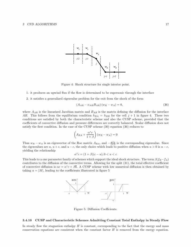
3 CFD ALGORITHMS 17

j-2

j

j+1 j+2

w w

w

ww

L L

A

RR

j-1

Figure 4: Shock structure for single interior point.

1. it produces an upwind flux if the flow is determined to be supersonic through the interface

2. it satisfies a generalized eigenvalue problem for the exit from the shock of the form

(AAR − αARBAR) (wR − wA) = 0, (36)

where AAR is the linearized Jacobian matrix and BAR is the matrix defining the diffusion for the interfaceAR. This follows from the equilibrium condition hRA = hRR for the cell j + 1 in figure 4. These twoconditions are satisfied by both the characteristic scheme and also the CUSP scheme, provided that thecoefficients of convective diffusion and pressure differences are correctly balanced. Scalar diffusion does notsatisfy the first condition. In the case of the CUSP scheme (30) equation (36) reduces to(

ARA +α∗c1 + β

)(wR − wA) = 0

Thus wR − wA is an eigenvector of the Roe matrix ARA, and − α∗c1+β is the corresponding eigenvalue. Since

the eigenvalues are u, u+ c, and u− c, the only choice which leads to positive diffusion when u > 0 is u− c,yielding the relationship

α∗c = (1 + β)(c− u), 0 < u < c

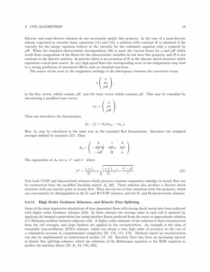
This leads to a one parameter family of schemes which support the ideal shock structure. The term β(fR−fA)contributes to the diffusion of the convective terms. Allowing for the split (31), the total effective coefficientof convective diffusion is αc = α∗c+ βu. A CUSP scheme with low numerical diffusion is then obtained bytaking α = |M |, leading to the coefficients illustrated in figure 5

α

1-1

1 1

-1

M M-1 1

(M) (M)β

Figure 5: Diffusion Coefficients.

3.4.10 CUSP and Characteristic Schemes Admitting Constant Total Enthalpy in Steady Flow

In steady flow the stagnation enthalpy H is constant, corresponding to the fact that the energy and massconservation equations are consistent when the constant factor H is removed from the energy equation.

3 CFD ALGORITHMS 18

Discrete and semi-discrete schemes do not necessarily satisfy this property. In the case of a semi-discretescheme expressed in viscosity form, equations (11) and (12), a solution with constant H is admitted if theviscosity for the energy equation reduces to the viscosity for the continuity equation with ρ replaced byρH . When the standard characteristic decomposition (28) is used, the viscous fluxes for ρ and ρH whichresult from composition of the fluxes for the characteristic variables do not have this property, and H is notconstant in the discrete solution. In practice there is an excursion of H in the discrete shock structure whichrepresents a local heat source. In very high speed flows the corresponding error in the temperature may leadto a wrong prediction of associated effects such as chemical reactions.

The source of the error in the stagnation enthalpy is the discrepancy between the convective terms

u

ρ

ρuρH

,

in the flux vector, which contain ρH , and the state vector which contains ρE. This may be remedied byintroducing a modified state vector

wh =

ρ

ρuρH

.

Then one introduces the linearization

fR − fL = Ah(whR − whL).

Here Ah may be calculated in the same way as the standard Roe linearization. Introduce the weightedaverages defined by equation (27). Then

Ah =

0 1 0

−γ+1γ

u2

2γ+1γ u γ−1

γ

−uH H u

.

The eigenvalues of Ah are u, λ+ and λ− where

λ± =γ + 12γ

u±√(γ + 12γ

u)2 +c2 − u2

γ. (37)

Now both CUSP and characteristic schemes which preserve constant stagnation enthalpy in steady flow canbe constructed from the modified Jacobian matrix Ah [88]. These schemes also produce a discrete shockstructure with one interior point in steady flow. Then one arrives at four variations with this property, whichcan conveniently be distinguished as the E- and H-CUSP schemes, and the E- and H-characteristic schemes.

3.4.11 High Order Godunov Schemes, and Kinetic Flux Splitting

Some of the most impressive simulations of time dependent flows with strong shock waves have been achievedwith higher order Godunov schemes [204]. In these schemes the average value in each cell is updated byapplying the integral conservation law using interface fluxes predicted from the exact or approximate solutionof a Riemann problem between adjacent cells. A higher order estimate of the solution is then reconstructedfrom the cell averages, and slope limiters are applied to the reconstruction. An example is the class ofessentially non-oscillatory (ENO) schemes, which can attain a very high order of accuracy at the cost ofa substantial increase in computational complexity [37, 173, 171, 172]. Methods based on reconstructioncan also be implemented on unstructured meshes [17, 16]. Recently there has been an increasing interestin kinetic flux splitting schemes, which use solutions of the Boltzmann equation or the BGK equation topredict the interface fluxes [50, 41, 54, 155, 205].

3 CFD ALGORITHMS 19

3.5 Multidimensional Schemes

The simplest approach to the treatment of multi-dimensional problems on structured meshes is to applythe one-dimensional construction separately in each mesh direction. On triangulated meshes in two orthree dimensions the SLIP and USLIP constructions may also be implemented along the mesh edges [87].A substantial body of current research is directed toward the implementation of truly multi-dimensionalupwind schemes in which the upwind biasing is determined by properties of the flow rather than the mesh[70, 154, 111, 46, 174]. A thorough review is given by Pailliere and DeConinck in reference [146].

Residual distribution schemes are an attractive approach for triangulated meshes. In these the residualdefined by the space derivatives is evaluated for each cell, and then distributed to the vertices with weightswhich depend on the direction of convection. For a scalar conservation law the weights can be chosen tomaintain positivity with minimum cross diffusion in the direction normal to the flow. For the Euler equationsthe residual can be linearized by assuming that the parameter vector with components

√ρ,√ρui, and

√ρH

varies linearly over the cell. Then∂fj(w)∂xj

= Aj∂w

∂xj

where the Jacobian matrices Aj =∂fj

∂w are evaluated with Roe averaging of the values of w at the vertices.Waves in the direction n can then be expressed in terms of the eigenvectors of njAj , and a positive distributionscheme is used for waves in preferred directions. The best choice of these directions is the subject of ongoingresearch, but preliminary results indicate the possibility of achieving high resolution of shocks and contactdiscontinuities which are not aligned with mesh lines [146].

Hirsch and Van Ransbeeck adopt an alternative approach in which they directly construct directionaldiffusive terms on structured meshes, with anti-diffusion controlled by limiters based on comparisons ofslopes in different directions [71]. They also show promising results in calculations of nozzles with multiplyreflected oblique shocks.

3.6 Discretization of the Viscous Terms

The discretization of the viscous terms of the Navier Stokes equations requires an approximation to thevelocity derivatives ∂ui

∂xjin order to calculate the tensor σij , equation (3). Then the viscous terms may be

included in the flux balance (4). In order to evaluate the derivatives one may apply the Gauss formula to acontrol volume V with the boundary S. ∫

V

∂ui

∂xjdv =

∫S

uinjds

where nj is the outward normal. For a tetrahedral or hexahedral cell this gives

∂ui

∂xj=

1vol

∑faces

ui nj s (38)

where ui is an estimate of the average of ui over the face. If u varies linearly over a tetrahedral cell this isexact. Alternatively, assuming a local transformation to computational coordinates ξj , one may apply thechain rule

∂u

∂x=[∂u

∂ξ

] [∂ξ

∂x

]=

∂u

∂ξ

[∂x

∂ξ

]−1

(39)

Here the transformation derivatives ∂xi

∂ξjcan be evaluated by the same finite difference formulas as the velocity

derivatives ∂ui

∂ξjIn this case ∂u

∂ξ is exact if u is a linearly varying function.For a cell-centered discretization (figure 6a) ∂u

∂ξ is needed at each face. The simplest procedure is toevaluate ∂u

∂ξ in each cell, and to average ∂u∂ξ between the two cells on either side of a face [97]. The resulting

discretization does not have a compact stencil, and supports undamped oscillatory modes. In a one dimen-sional calculation, for example, ∂2u

∂x2 would be discretized as ui+2−2ui+ui−24∆x2 . In order to produce a compact

3 CFD ALGORITHMS 20

stencil ∂u∂x may be estimated from a control volume centered on each face, using formulas (38) or (39) [163].

This is computationally expensive because the number of faces is much larger than the number of cells. Ina hexahedral mesh with a large number of vertices the number of faces approaches three times the numberof cells.

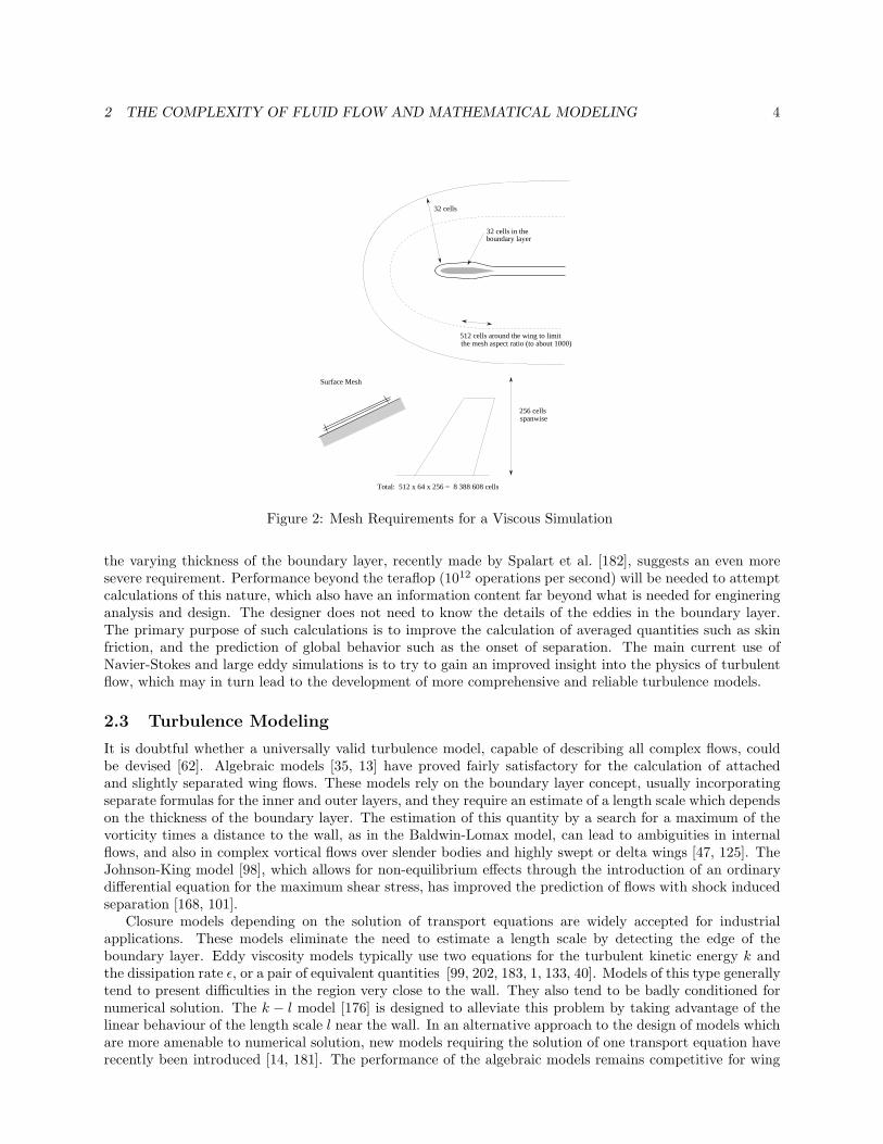
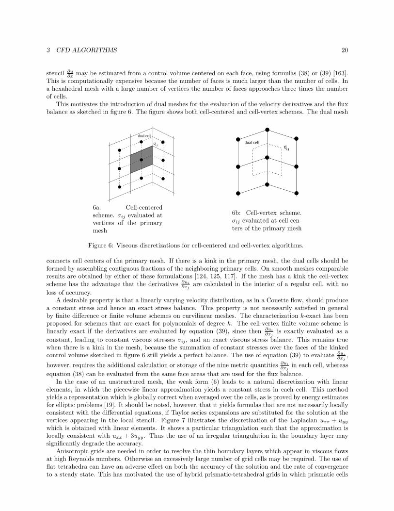
This motivates the introduction of dual meshes for the evaluation of the velocity derivatives and the fluxbalance as sketched in figure 6. The figure shows both cell-centered and cell-vertex schemes. The dual mesh

i jσ

dual cell

6a: Cell-centeredscheme. σij evaluated atvertices of the primarymesh

σi j

dual cell

6b: Cell-vertex scheme.σij evaluated at cell cen-ters of the primary mesh

Figure 6: Viscous discretizations for cell-centered and cell-vertex algorithms.

connects cell centers of the primary mesh. If there is a kink in the primary mesh, the dual cells should beformed by assembling contiguous fractions of the neighboring primary cells. On smooth meshes comparableresults are obtained by either of these formulations [124, 125, 117]. If the mesh has a kink the cell-vertexscheme has the advantage that the derivatives ∂ui

∂xjare calculated in the interior of a regular cell, with no

loss of accuracy.A desirable property is that a linearly varying velocity distribution, as in a Couette flow, should produce

a constant stress and hence an exact stress balance. This property is not necessarily satisfied in generalby finite difference or finite volume schemes on curvilinear meshes. The characterization k-exact has beenproposed for schemes that are exact for polynomials of degree k. The cell-vertex finite volume scheme islinearly exact if the derivatives are evaluated by equation (39), since then ∂ui

∂xjis exactly evaluated as a

constant, leading to constant viscous stresses σij , and an exact viscous stress balance. This remains truewhen there is a kink in the mesh, because the summation of constant stresses over the faces of the kinkedcontrol volume sketched in figure 6 still yields a perfect balance. The use of equation (39) to evaluate ∂ui

∂xj,

however, requires the additional calculation or storage of the nine metric quantities ∂ui

∂xjin each cell, whereas

equation (38) can be evaluated from the same face areas that are used for the flux balance.In the case of an unstructured mesh, the weak form (6) leads to a natural discretization with linear

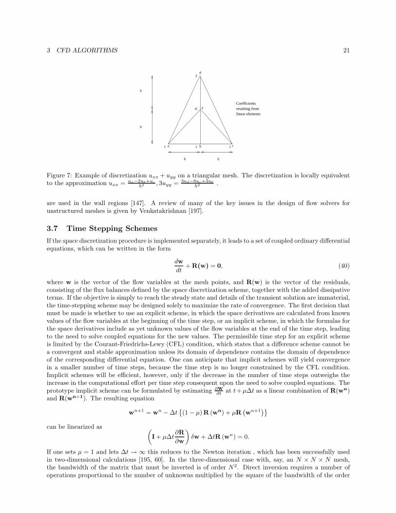
elements, in which the piecewise linear approximation yields a constant stress in each cell. This methodyields a representation which is globally correct when averaged over the cells, as is proved by energy estimatesfor elliptic problems [19]. It should be noted, however, that it yields formulas that are not necessarily locallyconsistent with the differential equations, if Taylor series expansions are substituted for the solution at thevertices appearing in the local stencil. Figure 7 illustrates the discretization of the Laplacian uxx + uyy

which is obtained with linear elements. It shows a particular triangulation such that the approximation islocally consistent with uxx + 3uyy. Thus the use of an irregular triangulation in the boundary layer maysignificantly degrade the accuracy.

Anisotropic grids are needed in order to resolve the thin boundary layers which appear in viscous flowsat high Reynolds numbers. Otherwise an excessively large number of grid cells may be required. The use offlat tetrahedra can have an adverse effect on both the accuracy of the solution and the rate of convergenceto a steady state. This has motivated the use of hybrid prismatic-tetrahedral grids in which prismatic cells

3 CFD ALGORITHMS 21

Coefficients resulting fromlinear elements

h

h

h

h

1 1 1a b c

d3

e-6

Figure 7: Example of discretization uxx + uyy on a triangular mesh. The discretization is locally equivalentto the approximation uxx = ua−2ub+uc

h2 , 3uyy = 3ud−6ue+3ub

h2 .

are used in the wall regions [147]. A review of many of the key issues in the design of flow solvers forunstructured meshes is given by Venkatakrishnan [197].

3.7 Time Stepping Schemes

If the space discretization procedure is implemented separately, it leads to a set of coupled ordinary differentialequations, which can be written in the form

dwdt

+R(w) = 0, (40)

where w is the vector of the flow variables at the mesh points, and R(w) is the vector of the residuals,consisting of the flux balances defined by the space discretization scheme, together with the added dissipativeterms. If the objective is simply to reach the steady state and details of the transient solution are immaterial,the time-stepping scheme may be designed solely to maximize the rate of convergence. The first decision thatmust be made is whether to use an explicit scheme, in which the space derivatives are calculated from knownvalues of the flow variables at the beginning of the time step, or an implicit scheme, in which the formulas forthe space derivatives include as yet unknown values of the flow variables at the end of the time step, leadingto the need to solve coupled equations for the new values. The permissible time step for an explicit schemeis limited by the Courant-Friedrichs-Lewy (CFL) condition, which states that a difference scheme cannot bea convergent and stable approximation unless its domain of dependence contains the domain of dependenceof the corresponding differential equation. One can anticipate that implicit schemes will yield convergencein a smaller number of time steps, because the time step is no longer constrained by the CFL condition.Implicit schemes will be efficient, however, only if the decrease in the number of time steps outweighs theincrease in the computational effort per time step consequent upon the need to solve coupled equations. Theprototype implicit scheme can be formulated by estimating ∂w

∂t at t+µ∆t as a linear combination of R(wn)and R(wn+1). The resulting equation

wn+1 = wn −∆t(1− µ)R (wn) + µR

(wn+1

)can be linearized as (

I+ µ∆t∂R∂w

)δw+∆tR (wn) = 0.

If one sets µ = 1 and lets ∆t → ∞ this reduces to the Newton iteration , which has been successfully usedin two-dimensional calculations [195, 60]. In the three-dimensional case with, say, an N × N × N mesh,the bandwidth of the matrix that must be inverted is of order N2. Direct inversion requires a number ofoperations proportional to the number of unknowns multiplied by the square of the bandwidth of the order

3 CFD ALGORITHMS 22

of N7. This is prohibitive, and forces recourse to either an approximate factorization method or an iterativesolution method.

Alternating direction methods, which introduce factors corresponding to each coordinate, are widely usedfor structured meshes [21, 156]. They cannot be implemented on unstructured tetrahedral meshes that donot contain identifiable mesh directions, although other decompositions are possible [67, 118]. If one choosesto adopt the iterative solution technique, the principal alternatives are variants of the Gauss-Seidel andJacobi methods. A symmetric Gauss-Seidel method with one iteration per time step is essentially equivalentto an approximate lower-upper (LU) factorization of the implicit scheme [96, 139, 36, 208]. On the otherhand, the Jacobi method with a fixed number of iterations per time step reduces to a multistage explicitscheme, belonging to the general class of Runge-Kutta schemes [38]. Schemes of this type have proved veryeffective for wide variety of problems, and they have the advantage that they can be applied equally easilyon both structured and unstructured meshes [95, 79, 81, 164].

If one reduces the linear model problem corresponding to (40) to an ordinary differential equation bysubstituting a Fourier mode w = eipxj , the resulting Fourier symbol has an imaginary part proportional tothe wave speed, and a negative real part proportional to the diffusion. Thus the time stepping scheme shouldhave a stability region which contains a substantial interval of the negative real axis, as well as an intervalalong the imaginary axis. To achieve this it pays to treat the convective and dissipative terms in a distinctfashion. Thus the residual is split as

R(w) = Q(w) +D(w),

where Q(w) is the convective part and D(w) the dissipative part. Denote the time level n∆t by a superscriptn. Then the multistage time stepping scheme is formulated as

w(n+1,0) = wn

. . .

w(n+1,k) = wn − αk∆t(Q(k−1) +D(k−1)

). . .

wn+1 = w(n+1,m),

where the superscript k denotes the k-th stage, αm = 1, and

Q(0) = Q (wn) , D(0) = D (wn). . .

Q(k) = Q(w(n+1,k)

)D(k) = βkD

(w(n+1,k)

)+ (1− βk)D(k−1).

The coefficients αk are chosen to maximize the stability interval along the imaginary axis, and the coefficientsβk are chosen to increase the stability interval along the negative real axis.

These schemes do not fall within the standard framework of Runge-Kutta schemes, and they have muchlarger stability regions [81]. Two schemes which have been found to be particularly effective are tabulatedbelow. The first is a four-stage scheme with two evaluations of dissipation. Its coefficients are

α1 = 13 β1 = 1

α2 = 415 β2 = 1

2α3 = 5

9 β3 = 0α4 = 1 β4 = 0

. (41)

The second is a five-stage scheme with three evaluations of dissipation. Its coefficients are

α1 = 14 β1 = 1

α2 = 16 β2 = 0

α3 = 38 β3 = 0.56

α4 = 12 β4 = 0

α5 = 1 β5 = 0.44

. (42)

3 CFD ALGORITHMS 23

3.8 Multigrid Methods

3.8.1 Acceleration of Steady Flow Calculations

Radical improvements in the rate of convergence to a steady state can be realized by the multigrid time-stepping technique. The concept of acceleration by the introduction of multiple grids was first proposed byFedorenko [57]. There is by now a fairly well-developed theory of multigrid methods for elliptic equationsbased on the concept that the updating scheme acts as a smoothing operator on each grid [28, 63]. Thistheory does not hold for hyperbolic systems. Nevertheless, it seems that it ought to be possible to acceleratethe evolution of a hyperbolic system to a steady state by using large time steps on coarse grids so thatdisturbances will be more rapidly expelled through the outer boundary. Various multigrid time-steppingschemes designed to take advantage of this effect have been proposed [138, 78, 65, 82, 34, 9, 68]

One can devise a multigrid scheme using a sequence of independently generated coarser meshes byeliminating alternate points in each coordinate direction. In order to give a precise description of themultigrid scheme, subscripts may be used to indicate the grid. Several transfer operations need to bedefined. First the solution vector on grid k must be initialized as

w(0)k = Tk,k−1wk−1,

where wk−1 is the current value on grid k − 1, and Tk,k−1 is a transfer operator. Next it is necessary totransfer a residual forcing function such that the solution grid k is driven by the residuals calculated on gridk − 1. This can be accomplished by setting

Pk = Qk,k−1Rk−1 (wk−1)−Rk

[w

(0)k

],

where Qk,k−1 is another transfer operator. Then Rk(wk) is replaced by Rk(wk) + Pk in the time- steppingscheme. Thus, the multistage scheme is reformulated as

w(1)k = w

(0)k − α1∆tk

[R

(0)k + Pk

]· · · · · ·

w(q+1)k = w

(0)k − αq+1∆tk

[R

(q)k + Pk

].

The result w(m)k then provides the initial data for grid k + 1. Finally, the accumulated correction on grid

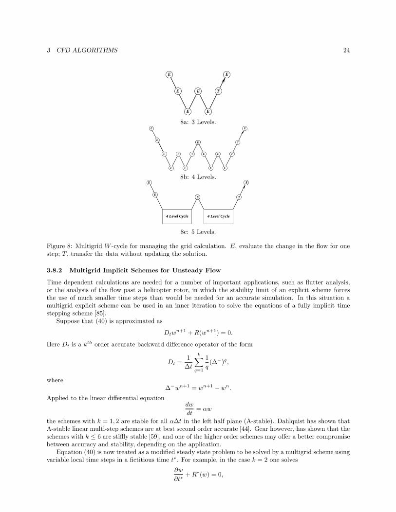
k has to be transferred back to grid k − 1 with the aid of an interpolation operator Ik−1,k. With properlyoptimized coefficients multistage time-stepping schemes can be very efficient drivers of the multigrid process.A W -cycle of the type illustrated in Figure 8 proves to be a particularly effective strategy for managing thework split between the meshes. In a three-dimensional case the number of cells is reduced by a factor ofeight on each coarser grid. On examination of the figure, it can therefore be seen that the work measured inunits corresponding to a step on the fine grid is of the order of

1 + 2/8 + 4/64 + . . . < 4/3,

and consequently the very large effective time step of the complete cycle costs only slightly more than asingle time step in the fine grid.

This procedure has proved extremely successful for the solution of the inviscid Euler equations, but lesseffective in calculations of turbulent viscous flows at high Reynolds numbers using the Reynolds averagedNavier Stokes equations. These require highly anisotropic grids with very fine mesh intervals normal to thewall to resolve the boundary layers. While simple multigrid methods still yield fast initial convergence, theytend to slow down as the calculation proceeds to a low asymptotic rate. This has motivated the introductionof semi-coarsening and directional coarsening methods [134, 135, 3, 4, 5, 150, 151].

The multigrid method can be applied on unstructured meshes by interpolating between a sequenceof separately generated meshes with progressively increasing cell sizes [94, 128, 129, 148]. It is not easyto generate very coarse meshes for complex configurations. An alternative approach, which removes thisdifficulty, is to automatically generate successively coarser meshes by agglomerating control volumes or bycollapsing edges. This approach yields comparable rates of convergence and has proved to be quite robust[103, 104, 130, 42].

3 CFD ALGORITHMS 24

E

E

E

E

T

E

E

8a: 3 Levels.

E

E

T

E

E

E

E

E

E

T

E

T E

E

E T

E

8b: 4 Levels.

E E T E

E E

4 Level Cycle 4 Level Cycle

8c: 5 Levels.

Figure 8: Multigrid W -cycle for managing the grid calculation. E, evaluate the change in the flow for onestep; T , transfer the data without updating the solution.

3.8.2 Multigrid Implicit Schemes for Unsteady Flow

Time dependent calculations are needed for a number of important applications, such as flutter analysis,or the analysis of the flow past a helicopter rotor, in which the stability limit of an explicit scheme forcesthe use of much smaller time steps than would be needed for an accurate simulation. In this situation amultigrid explicit scheme can be used in an inner iteration to solve the equations of a fully implicit timestepping scheme [85].

Suppose that (40) is approximated as

Dtwn+1 +R(wn+1) = 0.

Here Dt is a kth order accurate backward difference operator of the form

Dt =1∆t

k∑q=1

1q(∆−)q,

where∆−wn+1 = wn+1 − wn.

Applied to the linear differential equationdw

dt= αw

the schemes with k = 1, 2 are stable for all α∆t in the left half plane (A-stable). Dahlquist has shown thatA-stable linear multi-step schemes are at best second order accurate [44]. Gear however, has shown that theschemes with k ≤ 6 are stiffly stable [59], and one of the higher order schemes may offer a better compromisebetween accuracy and stability, depending on the application.

Equation (40) is now treated as a modified steady state problem to be solved by a multigrid scheme usingvariable local time steps in a fictitious time t∗. For example, in the case k = 2 one solves

∂w

∂t∗+R∗(w) = 0,

3 CFD ALGORITHMS 25

whereR∗(w) =

32∆t

w +R(w)− 2∆t

wn +1

2∆twn−1,

and the last two terms are treated as fixed source terms. The first term shifts the Fourier symbol of theequivalent model problem to the left in the complex plane. While this promotes stability, it may also requirea limit to be imposed on the magnitude of the local time step ∆t∗ relative to that of the implicit time step∆t. This may be relieved by a point-implicit modification of the multi-stage scheme [131]. In the case ofproblems with moving boundaries the equations must be modified to allow for movement and deformationof the mesh.

This method has proved effective for the calculation of unsteady flows that might be associated with wingflutter [6, 7] and also in the calculation of unsteady incompressible flows [22]. It has the advantage that itcan be added as an option to a computer program which uses an explicit multigrid scheme, allowing it to beused for the efficient calculation of both steady and unsteady flows. A similar approach has been successfullyadopted for unsteady flow simulations on unstructured grids by Venkatakrishnan and Mavriplis [198].

3.9 Preconditioning

Another way to improve the rate of convergence to a steady state is to multiply the space derivatives inequation (1) by a preconditioning matrix P which is designed to equalize the eigenvalues, so that all thewaves can be advanced with optimal time steps. A symmetric preconditioner which equalizes the eigenvalueshas been proposed by Van Leer [112]. When the equations are written in stream-aligned coordinates thishas the form

P =

τβ2M

2 − τβM 0 0 0

− τβM

τβ2 + 1 0 0 0

0 0 τ 0 00 0 0 τ 00 0 0 0 1

where

β = τ =√1−M2, if M < 1

β =√1−M2, τ =

√1− 1

M2, if M ≥ 1

Turkel has proposed an asymmetric preconditioner which has also proved effective, particularly for flow atlow Mach numbers [194]. The use of these preconditioners can lead to instability at stagnation points wherethere is a zero eigenvalue which cannot be equalized with the eigenvalues ±c.

The preconditioners of Van Leer and Turkel do not take account of the effect of differences in themesh intervals in the different coordinate directions. The need to resolve the boundary layer generallycompels the introduction of mesh cells with very high aspect ratios near the boundary, and these can leadto a severe reduction in the rate of convergence to a steady state. Allmaras has analyzed explicit andimplicit Jacobi-based preconditioners which include the influence of the mesh intervals [3, 4, 5]. Usinga block-Jacobi preconditioner with coarsening only in the direction normal to the wall, Pierce has recentlyobtained impressive results on viscous flows with high aspect ratio grids [150, 151]. Mavriplis has successfullycombined block preconditioners with line solvers to accelerate the convergence of viscous flow solutions onhighly stretched unstructured grids [127].

An alternative approach has recently been proposed by Ta’asan [190], in which the equations are writtenin a canonical form which separates the equations describing acoustic waves from those describing convection.In terms of the velocity components u, v and the vorticity ω, temperature T , entropy s and total enthalpy

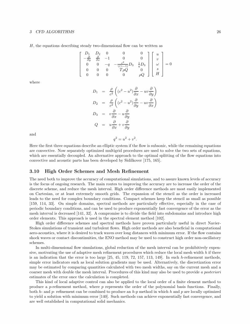
3 CFD ALGORITHMS 26

H , the equations describing steady two-dimensional flow can be written as

D1 D2 0 0 0− ∂

∂y∂∂x −1 0 0

0 0 −q − c2

γ(γ−1)D31qD3

0 0 0 TρQ 00 0 0 0 ρQ

uvωsH

= 0

where

D1 =ρ

c2

((c2 − u2)

∂

∂x− uv

∂

∂y

)

D2 =ρ

c2

((c2 − u2)

∂

∂y− uv

∂

∂x

)

D3 = v∂

∂x− u

∂

∂y

Q = u∂

∂x+ v

∂

∂y

andq2 = u2 + v2.

Here the first three equations describe an elliptic system if the flow is subsonic, while the remaining equationsare convective. Now separately optimized multigrid procedures are used to solve the two sets of equations,which are essentially decoupled. An alternative approach to the optimal splitting of the flow equations intoconvective and acoustic parts has been developed by Sidilkover [175, 165].

3.10 High Order Schemes and Mesh Refinement

The need both to improve the accuracy of computational simulations, and to assure known levels of accuracyis the focus of ongoing research. The main routes to improving the accuracy are to increase the order of thediscrete scheme, and reduce the mesh interval. High order difference methods are most easily implementedon Cartesian, or at least extremely smooth grids. The expansion of the stencil as the order is increasedleads to the need for complex boundary conditions. Compact schemes keep the stencil as small as possible[159, 114, 33]. On simple domains, spectral methods are particularly effective, especially in the case ofperiodic boundary conditions, and can be used to produce exponentially fast convergence of the error as themesh interval is decreased [141, 32]. A compromise is to divide the field into subdomains and introduce highorder elements. This approach is used in the spectral element method [102].

High order difference schemes and spectral methods have proven particularly useful in direct Navier-Stokes simulations of transient and turbulent flows. High order methods are also beneficial in computationalaero-acoustics, where it is desired to track waves over long distances with minimum error. If the flow containsshock waves or contact discontinuities, the ENO method may be used to construct high order non-oscillatoryschemes.

In multi-dimensional flow simulations, global reduction of the mesh interval can be prohibitively expen-sive, motivating the use of adaptive mesh refinement procedures which reduce the local mesh width h if thereis an indication that the error is too large [25, 45, 119, 72, 157, 113, 149]. In such h-refinement methods,simple error indicators such as local solution gradients may be used. Alternatively, the discretization errormay be estimated by comparing quantities calculated with two mesh widths, say on the current mesh and acoarser mesh with double the mesh interval. Procedures of this kind may also be used to provide a posterioriestimates of the error once the calculation is completed.

This kind of local adaptive control can also be applied to the local order of a finite element method toproduce a p-refinement method, where p represents the order of the polynomial basis functions. Finally,both h- and p- refinement can be combined to produce an h-p method in which h and p are locally optimizedto yield a solution with minimum error [140]. Such methods can achieve exponentially fast convergence, andare well established in computational solid mechanics.

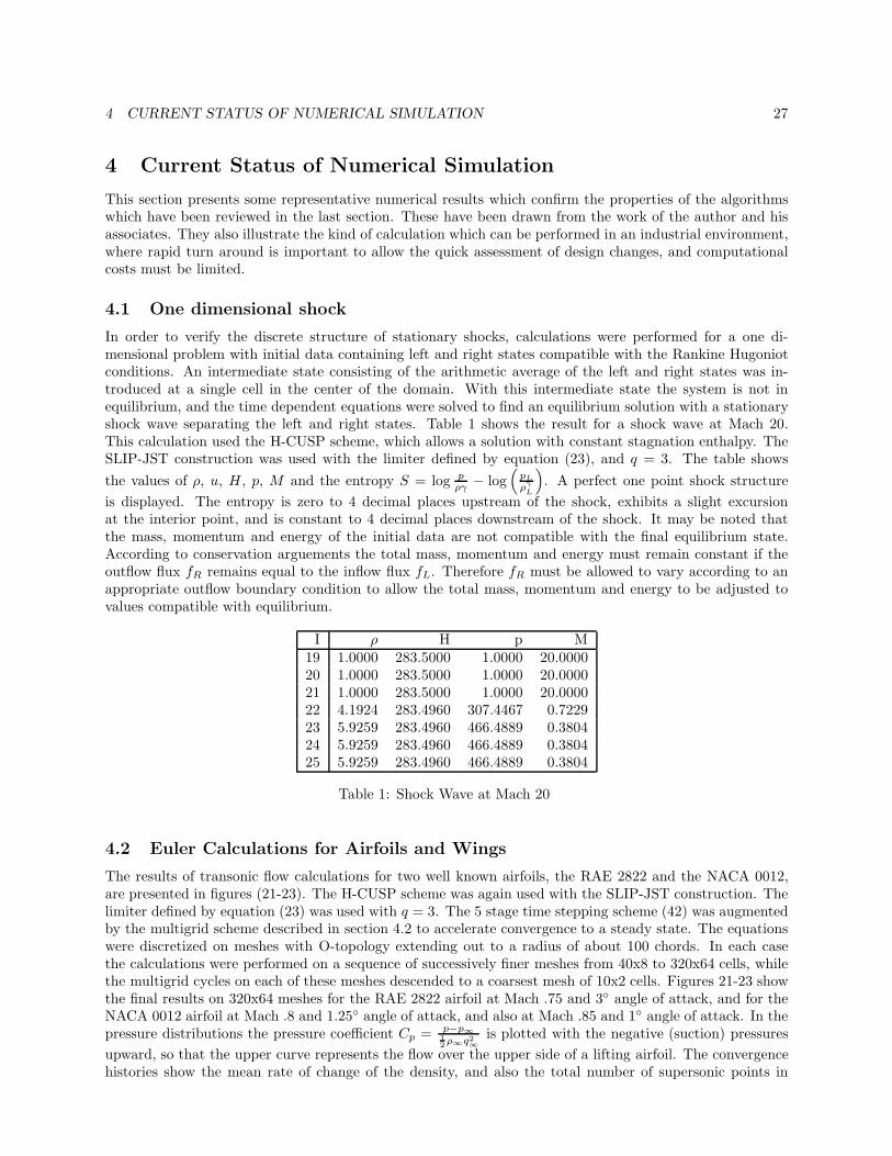
4 CURRENT STATUS OF NUMERICAL SIMULATION 27

4 Current Status of Numerical Simulation

This section presents some representative numerical results which confirm the properties of the algorithmswhich have been reviewed in the last section. These have been drawn from the work of the author and hisassociates. They also illustrate the kind of calculation which can be performed in an industrial environment,where rapid turn around is important to allow the quick assessment of design changes, and computationalcosts must be limited.

4.1 One dimensional shock

In order to verify the discrete structure of stationary shocks, calculations were performed for a one di-mensional problem with initial data containing left and right states compatible with the Rankine Hugoniotconditions. An intermediate state consisting of the arithmetic average of the left and right states was in-troduced at a single cell in the center of the domain. With this intermediate state the system is not inequilibrium, and the time dependent equations were solved to find an equilibrium solution with a stationaryshock wave separating the left and right states. Table 1 shows the result for a shock wave at Mach 20.This calculation used the H-CUSP scheme, which allows a solution with constant stagnation enthalpy. TheSLIP-JST construction was used with the limiter defined by equation (23), and q = 3. The table showsthe values of ρ, u, H , p, M and the entropy S = log p

ργ − log(

pL

ργL

). A perfect one point shock structure

is displayed. The entropy is zero to 4 decimal places upstream of the shock, exhibits a slight excursionat the interior point, and is constant to 4 decimal places downstream of the shock. It may be noted thatthe mass, momentum and energy of the initial data are not compatible with the final equilibrium state.According to conservation arguements the total mass, momentum and energy must remain constant if theoutflow flux fR remains equal to the inflow flux fL. Therefore fR must be allowed to vary according to anappropriate outflow boundary condition to allow the total mass, momentum and energy to be adjusted tovalues compatible with equilibrium.

I ρ H p M19 1.0000 283.5000 1.0000 20.000020 1.0000 283.5000 1.0000 20.000021 1.0000 283.5000 1.0000 20.000022 4.1924 283.4960 307.4467 0.722923 5.9259 283.4960 466.4889 0.380424 5.9259 283.4960 466.4889 0.380425 5.9259 283.4960 466.4889 0.3804

Table 1: Shock Wave at Mach 20

4.2 Euler Calculations for Airfoils and Wings

The results of transonic flow calculations for two well known airfoils, the RAE 2822 and the NACA 0012,are presented in figures (21-23). The H-CUSP scheme was again used with the SLIP-JST construction. Thelimiter defined by equation (23) was used with q = 3. The 5 stage time stepping scheme (42) was augmentedby the multigrid scheme described in section 4.2 to accelerate convergence to a steady state. The equationswere discretized on meshes with O-topology extending out to a radius of about 100 chords. In each casethe calculations were performed on a sequence of successively finer meshes from 40x8 to 320x64 cells, whilethe multigrid cycles on each of these meshes descended to a coarsest mesh of 10x2 cells. Figures 21-23 showthe final results on 320x64 meshes for the RAE 2822 airfoil at Mach .75 and 3 angle of attack, and for theNACA 0012 airfoil at Mach .8 and 1.25 angle of attack, and also at Mach .85 and 1 angle of attack. In thepressure distributions the pressure coefficient Cp = p−p∞

12ρ∞q2∞

is plotted with the negative (suction) pressuresupward, so that the upper curve represents the flow over the upper side of a lifting airfoil. The convergencehistories show the mean rate of change of the density, and also the total number of supersonic points in

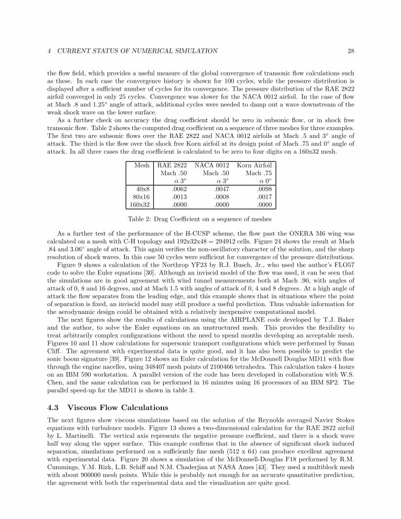
4 CURRENT STATUS OF NUMERICAL SIMULATION 28

the flow field, which provides a useful measure of the global convergence of transonic flow calculations suchas these. In each case the convergence history is shown for 100 cycles, while the pressure distribution isdisplayed after a sufficient number of cycles for its convergence. The pressure distribution of the RAE 2822airfoil converged in only 25 cycles. Convergence was slower for the NACA 0012 airfoil. In the case of flowat Mach .8 and 1.25 angle of attack, additional cycles were needed to damp out a wave downstream of theweak shock wave on the lower surface.

As a further check on accuracy the drag coefficient should be zero in subsonic flow, or in shock freetransonic flow. Table 2 shows the computed drag coefficient on a sequence of three meshes for three examples.The first two are subsonic flows over the RAE 2822 and NACA 0012 airfoils at Mach .5 and 3 angle ofattack. The third is the flow over the shock free Korn airfoil at its design point of Mach .75 and 0 angle ofattack. In all three cases the drag coefficient is calculated to be zero to four digits on a 160x32 mesh.

Mesh RAE 2822 NACA 0012 Korn AirfoilMach .50 Mach .50 Mach .75

α 3 α 3 α 0

40x8 .0062 .0047 .009880x16 .0013 .0008 .0017160x32 .0000 .0000 .0000

Table 2: Drag Coefficient on a sequence of meshes

As a further test of the performance of the H-CUSP scheme, the flow past the ONERA M6 wing wascalculated on a mesh with C-H topology and 192x32x48 = 294912 cells. Figure 24 shows the result at Mach.84 and 3.06 angle of attack. This again verifies the non-oscillatory character of the solution, and the sharpresolution of shock waves. In this case 50 cycles were sufficient for convergence of the pressure distributions.

Figure 9 shows a calculation of the Northrop YF23 by R.J. Busch, Jr., who used the author’s FLO57code to solve the Euler equations [30]. Although an inviscid model of the flow was used, it can be seen thatthe simulations are in good agreement with wind tunnel measurements both at Mach .90, with angles ofattack of 0, 8 and 16 degrees, and at Mach 1.5 with angles of attack of 0, 4 and 8 degrees. At a high angle ofattack the flow separates from the leading edge, and this example shows that in situations where the pointof separation is fixed, an inviscid model may still produce a useful prediction. Thus valuable information forthe aerodynamic design could be obtained with a relatively inexpensive computational model.

The next figures show the results of calculations using the AIRPLANE code developed by T.J. Bakerand the author, to solve the Euler equations on an unstructured mesh. This provides the flexibility totreat arbitrarily complex configurations without the need to spend months developing an acceptable mesh.Figures 10 and 11 show calculations for supersonic transport configurations which were performed by SusanCliff. The agreement with experimental data is quite good, and it has also been possible to predict thesonic boom signature [39]. Figure 12 shows an Euler calculation for the McDonnell Douglas MD11 with flowthrough the engine nacelles, using 348407 mesh points of 2100466 tetrahedra. This calculation takes 4 hourson an IBM 590 workstation. A parallel version of the code has been developed in collaboration with W.S.Chen, and the same calculation can be performed in 16 minutes using 16 processors of an IBM SP2. Theparallel speed-up for the MD11 is shown in table 3.

4.3 Viscous Flow Calculations

The next figures show viscous simulations based on the solution of the Reynolds averaged Navier Stokesequations with turbulence models. Figure 13 shows a two-dimensional calculation for the RAE 2822 airfoilby L. Martinelli. The vertical axis represents the negative pressure coefficient, and there is a shock wavehalf way along the upper surface. This example confirms that in the absence of significant shock inducedseparation, simulations performed on a sufficiently fine mesh (512 x 64) can produce excellent agreementwith experimental data. Figure 20 shows a simulation of the McDonnell-Douglas F18 performed by R.M.Cummings, Y.M. Rizk, L.B. Schiff and N.M. Chaderjian at NASA Ames [43]. They used a multiblock meshwith about 900000 mesh points. While this is probably not enough for an accurate quantitative prediction,the agreement with both the experimental data and the visualization are quite good.

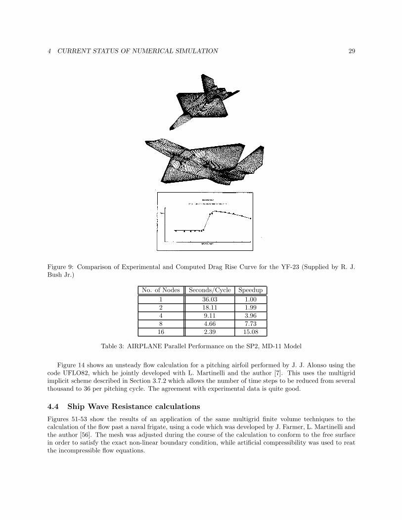
4 CURRENT STATUS OF NUMERICAL SIMULATION 29

Figure 9: Comparison of Experimental and Computed Drag Rise Curve for the YF-23 (Supplied by R. J.Bush Jr.)

No. of Nodes Seconds/Cycle Speedup1 36.03 1.002 18.11 1.994 9.11 3.968 4.66 7.7316 2.39 15.08

Table 3: AIRPLANE Parallel Performance on the SP2, MD-11 Model

Figure 14 shows an unsteady flow calculation for a pitching airfoil performed by J. J. Alonso using thecode UFLO82, which he jointly developed with L. Martinelli and the author [7]. This uses the multigridimplicit scheme described in Section 3.7.2 which allows the number of time steps to be reduced from severalthousand to 36 per pitching cycle. The agreement with experimental data is quite good.

4.4 Ship Wave Resistance calculations

Figures 51-53 show the results of an application of the same multigrid finite volume techniques to thecalculation of the flow past a naval frigate, using a code which was developed by J. Farmer, L. Martinelli andthe author [56]. The mesh was adjusted during the course of the calculation to conform to the free surfacein order to satisfy the exact non-linear boundary condition, while artificial compressibility was used to reatthe incompressible flow equations.

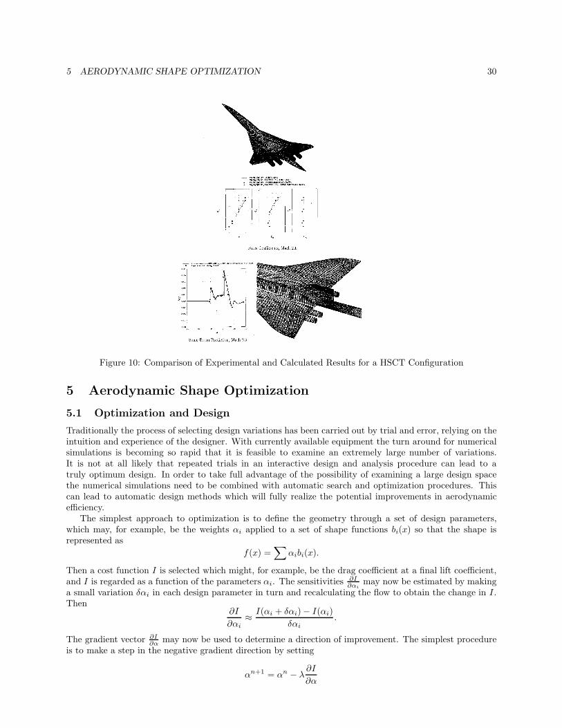
5 AERODYNAMIC SHAPE OPTIMIZATION 30

Figure 10: Comparison of Experimental and Calculated Results for a HSCT Configuration

5 Aerodynamic Shape Optimization

5.1 Optimization and Design

Traditionally the process of selecting design variations has been carried out by trial and error, relying on theintuition and experience of the designer. With currently available equipment the turn around for numericalsimulations is becoming so rapid that it is feasible to examine an extremely large number of variations.It is not at all likely that repeated trials in an interactive design and analysis procedure can lead to atruly optimum design. In order to take full advantage of the possibility of examining a large design spacethe numerical simulations need to be combined with automatic search and optimization procedures. Thiscan lead to automatic design methods which will fully realize the potential improvements in aerodynamicefficiency.

The simplest approach to optimization is to define the geometry through a set of design parameters,which may, for example, be the weights αi applied to a set of shape functions bi(x) so that the shape isrepresented as

f(x) =∑

αibi(x).

Then a cost function I is selected which might, for example, be the drag coefficient at a final lift coefficient,and I is regarded as a function of the parameters αi. The sensitivities ∂I

∂αimay now be estimated by making

a small variation δαi in each design parameter in turn and recalculating the flow to obtain the change in I.Then

∂I

∂αi≈ I(αi + δαi)− I(αi)

δαi.

The gradient vector ∂I∂α may now be used to determine a direction of improvement. The simplest procedure

is to make a step in the negative gradient direction by setting

αn+1 = αn − λ∂I

∂α

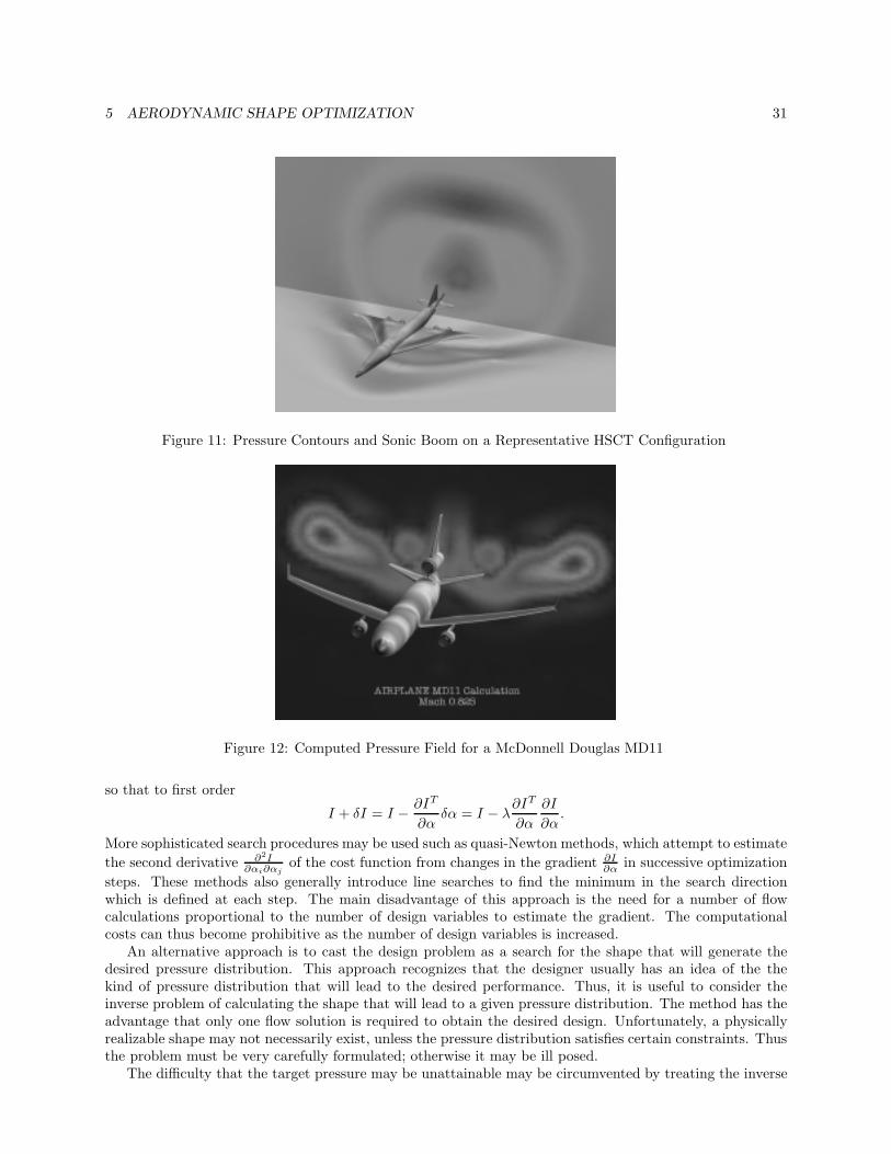
5 AERODYNAMIC SHAPE OPTIMIZATION 31

Figure 11: Pressure Contours and Sonic Boom on a Representative HSCT Configuration

Figure 12: Computed Pressure Field for a McDonnell Douglas MD11

so that to first order

I + δI = I − ∂IT

∂αδα = I − λ

∂IT

∂α

∂I

∂α.

More sophisticated search procedures may be used such as quasi-Newton methods, which attempt to estimatethe second derivative ∂2I

∂αi∂αjof the cost function from changes in the gradient ∂I

∂α in successive optimizationsteps. These methods also generally introduce line searches to find the minimum in the search directionwhich is defined at each step. The main disadvantage of this approach is the need for a number of flowcalculations proportional to the number of design variables to estimate the gradient. The computationalcosts can thus become prohibitive as the number of design variables is increased.

An alternative approach is to cast the design problem as a search for the shape that will generate thedesired pressure distribution. This approach recognizes that the designer usually has an idea of the thekind of pressure distribution that will lead to the desired performance. Thus, it is useful to consider theinverse problem of calculating the shape that will lead to a given pressure distribution. The method has theadvantage that only one flow solution is required to obtain the desired design. Unfortunately, a physicallyrealizable shape may not necessarily exist, unless the pressure distribution satisfies certain constraints. Thusthe problem must be very carefully formulated; otherwise it may be ill posed.

The difficulty that the target pressure may be unattainable may be circumvented by treating the inverse

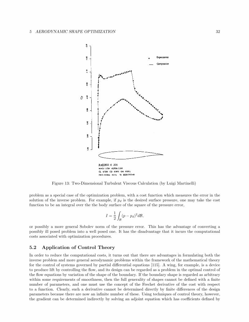
5 AERODYNAMIC SHAPE OPTIMIZATION 32

Figure 13: Two-Dimensional Turbulent Viscous Calculation (by Luigi Martinelli)

problem as a special case of the optimization problem, with a cost function which measures the error in thesolution of the inverse problem. For example, if pd is the desired surface pressure, one may take the costfunction to be an integral over the the body surface of the square of the pressure error,

I =12

∫B(p− pd)2dB,

or possibly a more general Sobolev norm of the pressure error. This has the advantage of converting apossibly ill posed problem into a well posed one. It has the disadvantage that it incurs the computationalcosts associated with optimization procedures.

5.2 Application of Control Theory

In order to reduce the computational costs, it turns out that there are advantages in formulating both theinverse problem and more general aerodynamic problems within the framework of the mathematical theoryfor the control of systems governed by partial differential equations [115]. A wing, for example, is a deviceto produce lift by controlling the flow, and its design can be regarded as a problem in the optimal control ofthe flow equations by variation of the shape of the boundary. If the boundary shape is regarded as arbitrarywithin some requirements of smoothness, then the full generality of shapes cannot be defined with a finitenumber of parameters, and one must use the concept of the Frechet derivative of the cost with respectto a function. Clearly, such a derivative cannot be determined directly by finite differences of the designparameters because there are now an infinite number of these. Using techniques of control theory, however,the gradient can be determined indirectly by solving an adjoint equation which has coefficients defined by

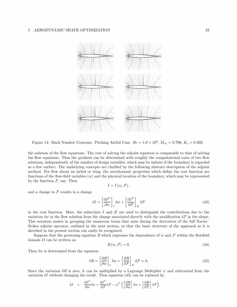
5 AERODYNAMIC SHAPE OPTIMIZATION 33

Figure 14: Mach Number Contours. Pitching Airfoil Case. Re = 1.0× 106, M∞ = 0.796, Kc = 0.202.

the solution of the flow equations. The cost of solving the adjoint equation is comparable to that of solvingthe flow equations. Thus the gradient can be determined with roughly the computational costs of two flowsolutions, independently of the number of design variables, which may be infinite if the boundary is regardedas a free surface. The underlying concepts are clarified by the following abstract description of the adjointmethod. For flow about an airfoil or wing, the aerodynamic properties which define the cost function arefunctions of the flow-field variables (w) and the physical location of the boundary, which may be representedby the function F , say. Then

I = I (w,F) ,and a change in F results in a change

δI =[∂IT

∂w

]I

δw +[∂IT

∂F]II

δF (43)

in the cost function. Here, the subscripts I and II are used to distinguish the contributions due to thevariation δw in the flow solution from the change associated directly with the modification δF in the shape.This notation assists in grouping the numerous terms that arise during the derivation of the full Navier–Stokes adjoint operator, outlined in the next section, so that the basic structure of the approach as it issketched in the present section can easily be recognized.

Suppose that the governing equation R which expresses the dependence of w and F within the flowfielddomain D can be written as

R (w,F) = 0. (44)

Then δw is determined from the equation

δR =[∂R

∂w

]I

δw +[∂R

∂F]II

δF = 0. (45)

Since the variation δR is zero, it can be multiplied by a Lagrange Multiplier ψ and subtracted from thevariation δI without changing the result. Thus equation (43) can be replaced by

δI =∂IT

∂wδw +

∂IT

∂F δF − ψT([∂R

∂w

]δw +

[∂R

∂F]δF)

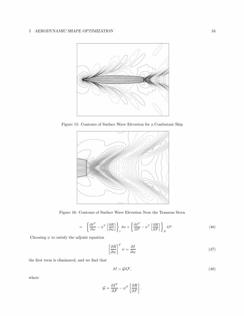
5 AERODYNAMIC SHAPE OPTIMIZATION 34

Figure 15: Contours of Surface Wave Elevation for a Combatant Ship

Figure 16: Contours of Surface Wave Elevation Near the Transom Stern

=

∂IT

∂w− ψT

[∂R

∂w

]I

δw +

∂IT

∂F − ψT[∂R

∂F]

II

δF . (46)

Choosing ψ to satisfy the adjoint equation

[∂R

∂w

]Tψ =

∂I

∂w(47)

the first term is eliminated, and we find that

δI = GδF , (48)

where

G =∂IT

∂F − ψT

[∂R

∂F].

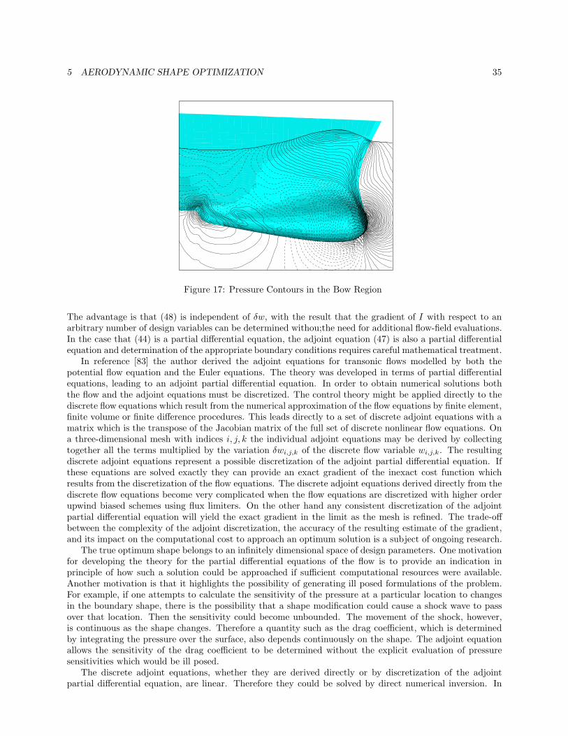
5 AERODYNAMIC SHAPE OPTIMIZATION 35

Figure 17: Pressure Contours in the Bow Region

The advantage is that (48) is independent of δw, with the result that the gradient of I with respect to anarbitrary number of design variables can be determined withou;the need for additional flow-field evaluations.In the case that (44) is a partial differential equation, the adjoint equation (47) is also a partial differentialequation and determination of the appropriate boundary conditions requires careful mathematical treatment.

In reference [83] the author derived the adjoint equations for transonic flows modelled by both thepotential flow equation and the Euler equations. The theory was developed in terms of partial differentialequations, leading to an adjoint partial differential equation. In order to obtain numerical solutions boththe flow and the adjoint equations must be discretized. The control theory might be applied directly to thediscrete flow equations which result from the numerical approximation of the flow equations by finite element,finite volume or finite difference procedures. This leads directly to a set of discrete adjoint equations with amatrix which is the transpose of the Jacobian matrix of the full set of discrete nonlinear flow equations. Ona three-dimensional mesh with indices i, j, k the individual adjoint equations may be derived by collectingtogether all the terms multiplied by the variation δwi,j,k of the discrete flow variable wi,j,k. The resultingdiscrete adjoint equations represent a possible discretization of the adjoint partial differential equation. Ifthese equations are solved exactly they can provide an exact gradient of the inexact cost function whichresults from the discretization of the flow equations. The discrete adjoint equations derived directly from thediscrete flow equations become very complicated when the flow equations are discretized with higher orderupwind biased schemes using flux limiters. On the other hand any consistent discretization of the adjointpartial differential equation will yield the exact gradient in the limit as the mesh is refined. The trade-offbetween the complexity of the adjoint discretization, the accuracy of the resulting estimate of the gradient,and its impact on the computational cost to approach an optimum solution is a subject of ongoing research.

The true optimum shape belongs to an infinitely dimensional space of design parameters. One motivationfor developing the theory for the partial differential equations of the flow is to provide an indication inprinciple of how such a solution could be approached if sufficient computational resources were available.Another motivation is that it highlights the possibility of generating ill posed formulations of the problem.For example, if one attempts to calculate the sensitivity of the pressure at a particular location to changesin the boundary shape, there is the possibility that a shape modification could cause a shock wave to passover that location. Then the sensitivity could become unbounded. The movement of the shock, however,is continuous as the shape changes. Therefore a quantity such as the drag coefficient, which is determinedby integrating the pressure over the surface, also depends continuously on the shape. The adjoint equationallows the sensitivity of the drag coefficient to be determined without the explicit evaluation of pressuresensitivities which would be ill posed.

The discrete adjoint equations, whether they are derived directly or by discretization of the adjointpartial differential equation, are linear. Therefore they could be solved by direct numerical inversion. In

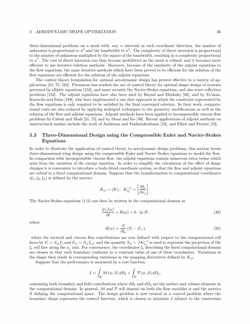
5 AERODYNAMIC SHAPE OPTIMIZATION 36

three-dimensional problems on a mesh with, say, n intervals in each coordinate direction, the number ofunknowns is proportional to n3 and the bandwidth to n2. The complexity of direct inversion is proportionalto the number of unknowns multiplied by the square of the bandwidth, resulting in a complexity proportionalto n7. The cost of direct inversion can thus become prohibitive as the mesh is refined, and it becomes moreefficient to use iterative solution methods. Moreover, because of the similarity of the adjoint equations tothe flow equations, the same iterative methods which have been proved to be efficient for the solution of theflow equations are efficient for the solution of the adjoint equations.

The control theory formulation for optimal aerodynamic design has proved effective in a variety of ap-plications [84, 75, 162]. Pironneau has studied the use of control theory for optimal shape design of systemsgoverned by elliptic equations [153], and more recently the Navier-Stokes equations, and also wave reflectionproblems [152]. The adjoint equations have also been used by Baysal and Eleshaky [20], and by Ta’asan,Kuruvila and Salas [189], who have implemented a one shot approach in which the constraint represented bythe flow equations is only required to be satisfied by the final converged solution. In their work, computa-tional costs are also reduced by applying multigrid techniques to the geometry modifications as well as thesolution of the flow and adjoint equations. Adjoint methods have been applied to incompressible viscous flowproblems by Cabuk and Modi [31, 73] and by Desai and Ito [49]. Recent applications of adjoint methods onunstructured meshes include the work of Anderson and Venkatakrishnan [10], and Elliot and Peraire [53].

5.3 Three-Dimensional Design using the Compressible Euler and Navier-StokesEquations

In order to illustrate the application of control theory to aerodynamic design problems, this section treatsthree-dimensional wing design using the compressible Euler and Navier Stokes equations to model the flow.In comparison with incompressible viscous flow, the adjoint equations contain numerous extra terms whicharise from the variation of the energy equation. In order to simplify the calculation of the effect of shapechanges it is convenient to introduce a body-fitted coordinate system, so that the flow and adjoint equationsare solved in a fixed computational domain. Suppose that the transformation to computational coordinates(ξ1, ξ2, ξ3) is defined by the metrics

Kij = (K) , K−1ij =

[∂ξi∂xj

].

The Navier-Stokes equations (1-3) can then be written in the computational domain as

∂ (Jw)∂t

+R(w) = 0 in D, (49)

whereR(w) =

∂

∂ξi(Fi − Fvi) (50)

where the inviscid and viscous flux contributions are now defined with respect to the computational cellfaces by Fi = Sijfj and Fvi = Sijfvj , and the quantity Sij = JK−1

ij is used to represent the projection of theξi cell face along the xj axis. For convenience, the coordinates ξi describing the fixed computational domainare chosen so that each boundary conforms to a constant value of one of these coordinates. Variations inthe shape then result in corresponding variations in the mapping derivatives defined by Kij .

Suppose that the performance is measured by a cost function

I =∫BM (w, S) dBξ +

∫DP (w, S) dDξ,

containing both boundary and field contributions where dBξ and dDξ are the surface and volume elements inthe computational domain. In general, M and P will depend on both the flow variables w and the metricsS defining the computational space. The design problem is now treated as a control problem where theboundary shape represents the control function, which is chosen to minimize I subject to the constraints

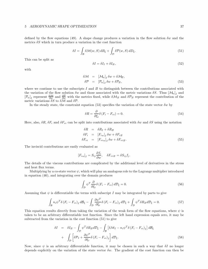
5 AERODYNAMIC SHAPE OPTIMIZATION 37

defined by the flow equations (49). A shape change produces a variation in the flow solution δw and themetrics δS which in turn produce a variation in the cost function

δI =∫BδM(w, S) dBξ +

∫DδP(w, S) dDξ. (51)

This can be split asδI = δII + δIII , (52)

with

δM = [Mw]I δw + δMII ,

δP = [Pw]I δw + δPII , (53)

where we continue to use the subscripts I and II to distinguish between the contributions associated withthe variation of the flow solution δw and those associated with the metric variations δS. Thus [Mw]I and[Pw]I represent ∂M

∂w and ∂P∂w with the metrics fixed, while δMII and δPII represent the contribution of the

metric variations δS to δM and δP .In the steady state, the constraint equation (53) specifies the variation of the state vector δw by

δR =∂

∂ξiδ (Fi − Fvi) = 0. (54)

Here, also, δR, δFi and δFvi can be split into contributions associated with δw and δS using the notation

δR = δRI + δRII

δFi = [Fiw]I δw + δFiII

δFvi = [Fviw]I δw + δFviII . (55)

The inviscid contributions are easily evaluated as

[Fiw]I = Sij∂fi∂w

, δFviII = δSijfj.

The details of the viscous contributions are complicated by the additional level of derivatives in the stressand heat flux terms.

Multiplying by a co-state vector ψ, which will play an analogous role to the Lagrangemultiplier introducedin equation (46), and integrating over the domain produces∫

DψT ∂

∂ξiδ (Fi − Fvi) dDξ = 0. (56)

Assuming that ψ is differentiable the terms with subscript I may be integrated by parts to give∫Bniψ

T δ (Fi − Fvi)I dBξ −∫D

∂ψT

∂ξiδ (Fi − Fvi)I dDξ +

∫DψT δRIIdDξ = 0. (57)

This equation results directly from taking the variation of the weak form of the flow equations, where ψ istaken to be an arbitrary differentiable test function. Since the left hand expression equals zero, it may besubtracted from the variation in the cost function (51) to give

δI = δIII −∫DψT δRIIdDξ −

∫B

[δMI − niψ

T δ (Fi − Fvi)I]dBξ

+∫D

[δPI +

∂ψT

∂ξiδ (Fi − Fvi)I

]dDξ. (58)

Now, since ψ is an arbitrary differentiable function, it may be chosen in such a way that δI no longerdepends explicitly on the variation of the state vector δw. The gradient of the cost function can then be

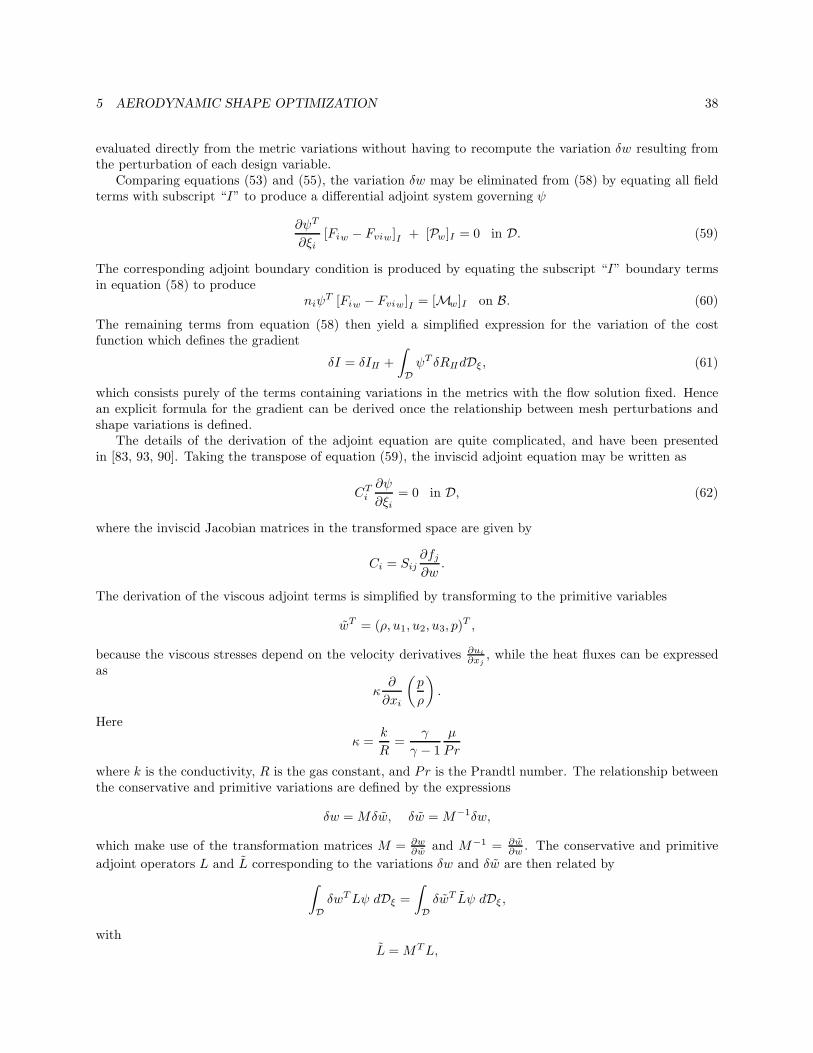
5 AERODYNAMIC SHAPE OPTIMIZATION 38

evaluated directly from the metric variations without having to recompute the variation δw resulting fromthe perturbation of each design variable.

Comparing equations (53) and (55), the variation δw may be eliminated from (58) by equating all fieldterms with subscript “I” to produce a differential adjoint system governing ψ

∂ψT

∂ξi[Fiw − Fviw]I + [Pw]I = 0 in D. (59)

The corresponding adjoint boundary condition is produced by equating the subscript “I” boundary termsin equation (58) to produce

niψT [Fiw − Fviw]I = [Mw]I on B. (60)

The remaining terms from equation (58) then yield a simplified expression for the variation of the costfunction which defines the gradient

δI = δIII +∫DψT δRIIdDξ, (61)

which consists purely of the terms containing variations in the metrics with the flow solution fixed. Hencean explicit formula for the gradient can be derived once the relationship between mesh perturbations andshape variations is defined.

The details of the derivation of the adjoint equation are quite complicated, and have been presentedin [83, 93, 90]. Taking the transpose of equation (59), the inviscid adjoint equation may be written as

CTi

∂ψ

∂ξi= 0 in D, (62)

where the inviscid Jacobian matrices in the transformed space are given by

Ci = Sij∂fj∂w

.

The derivation of the viscous adjoint terms is simplified by transforming to the primitive variables

wT = (ρ, u1, u2, u3, p)T ,

because the viscous stresses depend on the velocity derivatives ∂ui

∂xj, while the heat fluxes can be expressed

as

κ∂

∂xi

(p

ρ

).

Hereκ =

k

R=

γ

γ − 1µ

Pr

where k is the conductivity, R is the gas constant, and Pr is the Prandtl number. The relationship betweenthe conservative and primitive variations are defined by the expressions

δw = Mδw, δw = M−1δw,

which make use of the transformation matrices M = ∂w∂w and M−1 = ∂w

∂w . The conservative and primitiveadjoint operators L and L corresponding to the variations δw and δw are then related by∫

DδwTLψ dDξ =

∫DδwT Lψ dDξ,

withL = MTL,

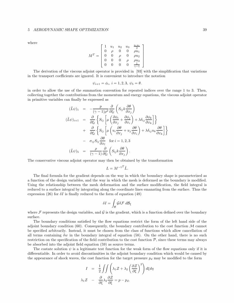
5 AERODYNAMIC SHAPE OPTIMIZATION 39

where

MT =

1 u1 u2 u3uiui

20 ρ 0 0 ρu1

0 0 ρ 0 ρu2

0 0 0 ρ ρu3

0 0 0 0 1γ−1

The derivation of the viscous adjoint operator is provided in [93] with the simplification that variationsin the transport coefficients are ignored. It is convenient to introduce the notation

ψi+1 = φi, i = 1, 2, 3, ψ5 = θ.

in order to allow the use of the summation convention for repeated indices over the range 1 to 3. Then,collecting together the contributions from the momentum and energy equations, the viscous adjoint operatorin primitive variables can finally be expressed as

(Lψ)1 = − p

(γ − 1)ρ2

∂

∂ξl

(Sljk

∂θ

∂xj

)

(Lψ)i+1 =∂

∂ξl

Slj

[µ

(∂φi

∂xj+

∂φj

∂xi

)+ λδij

∂φk

∂xk

]

+∂

∂ξl

Slj

[µ

(ui

∂θ

∂xj+ uj

∂θ

∂xi

)+ λδijuk

∂θ

∂xk

]

− σijSlj∂θ

∂xlfor i = 1, 2, 3

(Lψ)5 =ρ

(γ − 1)∂

∂ξl

(Sljk

∂θ

∂xj

).

The conservative viscous adjoint operator may then be obtained by the transformation

L = M−1T L.

The final formula for the gradient depends on the way in which the boundary shape is parameterized asa function of the design variables, and the way in which the mesh is deformed as the boundary is modified.Using the relationship between the mesh deformation and the surface modification, the field integral isreduced to a surface integral by integrating along the coordinate lines emanating from the surface. Thus theexpression (26) for δI is finally reduced to the form of equation (48)

δI =∫BGδF dBξ

where F represents the design variables, and G is the gradient, which is a function defined over the boundarysurface.

The boundary conditions satisfied by the flow equations restrict the form of the left hand side of theadjoint boundary condition (60). Consequently, the boundary contribution to the cost function M cannotbe specified arbitrarily. Instead, it must be chosen from the class of functions which allow cancellation ofall terms containing δw in the boundary integral of equation (58). On the other hand, there is no suchrestriction on the specification of the field contribution to the cost function P , since these terms may alwaysbe absorbed into the adjoint field equation (59) as source terms.

The costate solution ψ is a legitimate test function for the weak form of the flow equations only if it isdifferentiable. In order to avoid discontinuities in the adjoint boundary condition which would be caused bythe appearance of shock waves, the cost function for the target pressure pd may be modified to the form

I =12

∫ ∫ (λ1Z + λ2

(∂Z∂ξ

)2)

dξdη

λ1Z − ∂

∂ξλ2

∂Z∂ξ

= p− pd.

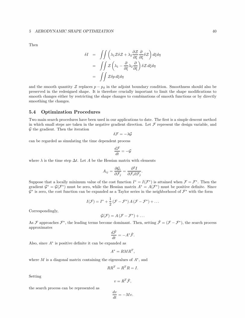
5 AERODYNAMIC SHAPE OPTIMIZATION 40

Then

δI =∫ ∫ (

λ1ZδZ + λ2∂Z∂ξ

∂

∂ξδZ)

dξdη

=∫ ∫

Z(λ1 − ∂

∂ξλ2

∂

∂ξ

)δZ dξdη

=∫ ∫

Zδp dξdη

and the smooth quantity Z replaces p − pd in the adjoint boundary condition. Smoothness should also bepreserved in the redesigned shape. It is therefore crucially important to limit the shape modifications tosmooth changes either by restricting the shape changes to combinations of smooth functions or by directlysmoothing the changes.

5.4 Optimization Procedures

Two main search procedures have been used in our applications to date. The first is a simple descent methodin which small steps are taken in the negative gradient direction. Let F represent the design variable, andG the gradient. Then the iteration

δF = −λGcan be regarded as simulating the time dependent process

dFdt

= −G

where λ is the time step ∆t. Let A be the Hessian matrix with elements

Aij =∂Gi

∂Fj=

∂2I

∂Fi∂Fj.

Suppose that a locally minimum value of the cost function I∗ = I(F∗) is attained when F = F∗. Then thegradient G∗ = G(F∗) must be zero, while the Hessian matrix A∗ = A(F∗) must be positive definite. SinceG∗ is zero, the cost function can be expanded as a Taylor series in the neighborhood of F∗ with the form

I(F) = I∗ +12(F − F∗)A (F − F∗) + . . .

Correspondingly,G(F) = A (F − F∗) + . . .

As F approaches F∗, the leading terms become dominant. Then, setting F = (F −F∗), the search processapproximates

dFdt

= −A∗F .

Also, since A∗ is positive definite it can be expanded as

A∗ = RMRT ,

where M is a diagonal matrix containing the eigenvalues of A∗, and

RRT = RTR = I.

Settingv = RT F ,

the search process can be represented asdv

dt= −Mv.

5 AERODYNAMIC SHAPE OPTIMIZATION 41

The stability region for the simple forward Euler stepping scheme is a unit circle centered at −1 on thenegative real axis. Thus for stability we must choose

µmax∆t = µmaxλ < 2,

while the asymptotic decay rate, given by the smallest eigenvalue, is proportional to

e−µmint.

In order to make sure that each new shape in the optimization sequence remains smooth, it provesessential to smooth the gradient and to replace G by its smoothed value G in the descent process. This alsoacts as a preconditioner which allows the use of much larger steps. To apply smoothing in the ξ1 direction,for example, the smoothed gradient G ma be calculated from a discrete approximation to

G − ∂

∂ξ1ε

∂

∂ξ1G = G

where ε is the smoothing parameter. If one sets δF = −λG, then, assuming the modification is applied onthe surface ξ2 = constant, the first order change in the cost function is

δI = −∫ ∫

GδF dξ1dξ3

= −λ

∫ ∫ (G − ∂

∂ξ1ε∂G∂ξ1

)G dξ1dξ3

= −λ

∫ ∫ (G2 + ε

(∂G∂ξ1

)2)

dξ1dξ3

< 0,

assuring an improvement if λ is sufficiently small and positive, unless the process has already reached astationary point at which G = 0.

It turns out that this approach is tolerant to the use of approximate values of the gradient, so thatneither the flow solution nor the adjoint solution need be fully converged before making a shape change.This results in very large savings in the computational cost. For inviscid optimization it is necessary to useonly 15 multigrid cycles for the flow solution and the adjoint solution in each design iteration. For viscousoptimization, about 100 multigrid cycles are needed. This is partly because convergence of the lift coefficientis much slower, so about 20 iterations must be made before each adjustment of the angle of attack to forcethe target lift coefficient.

Our second main search procedure incorporates a quasi-Newton method for general constrained opti-mization. In this class of methods the step is defined as

δF = −λPG,where P is a preconditioner for the search. An ideal choice is P = A∗−1, so that the corresponding timedependent process reduces to

dFdt

= −F ,

for which all the eigenvalues are equal to unity, and F is reduced to zero in one time step by the choice∆t = 1 if the Hessian, A, is constant. The full Newton method takes P = A−1, requiring the evaluationof the Hessian matrix, A, at each step. It corresponds to the use of the Newton-Raphson method to solvethe non-linear equation G = 0. Quasi-Newton methods estimate A∗ from the change in the gradient duringthe search process. This requires accurate estimates of the gradient at each time step. In order to obtainthese, both the flow solution and the adjoint equation must be fully converged. Most quasi-Newton methodsalso require a line search in each search direction, for which the flow equations and cost function mustbe accurately evaluated several times. Since the Hessian can only be completely estimated after as many

5 AERODYNAMIC SHAPE OPTIMIZATION 42

steps as there are design variables, it pays to reduce the number of design variables with this approach byrepresenting the geometry as a superposition of appropriately chosen shape functions. The Hicks-Hennebump functions [162] have proved effective in many applications. Because those functions are smooth theyalso serve the purpose of preserving the smoothness of the shape modifications, which is essential for anyacceptable design.

In the applications to complex configurations presented below the optimization was carried out usingthe existing, well validated software NPSOL. This software, which implements a quasi-Newton method foroptimization with both linear and non-linear constraints, has proved very reliable but is generally moreexpensive than the simple search method with smoothing.

5.5 Industrial Experience and Results of Optimization

The methods described in this paper have been quite thoroughly tested in industrial applications in whichthey were used as a tool for aerodynamic design. They have proved useful both in inverse mode to findshapes that would produce desired pressure distributions, and for direct minimization of the drag. Theyhave been applied both to well understood configurations that have gradually evolved through incrementalimprovements guided by wind tunnel tests and computational simulation, and to new concepts for whichthere is a limited knowledge base. In either case they have enabled engineers to produce improved designs.

Substantial improvements are usually obtained with 20 − 200 design cycles, depending on the difficultyof the case. One concern is the possibility of getting trapped in a local minimum. In practice this hasnot proved to be a source of difficulty. In inverse mode, it often proves possible to come very close torealizing the target pressure distribution, thus effectively demonstrating convergence. In drag minimization,the result of the optimization is usually a shock-free wing. If one considers drag minimization of airfoils intwo-dimensional inviscid transonic flow, it can be seen that every shock-free airfoil produces zero drag, andthus optimization based solely on drag has a highly non-unique solution. Different shock-free airfoils can beobtained by starting from different initial profiles. One may also influence the character of the final designby blending a target pressure distribution with the drag in the definition of the cost function.

Similar considerations apply to three-dimensional wing design in viscous transonic flow. Since the vortexdrag can be reduced simply by reducing the lift, the lift coefficient must be fixed for a meaningful dragminimization. A typical wing of a transport aircraft is designed for a lift coefficient in the range of 0.4 to 0.6.The total wing drag may be broken down into vortex drag, drag due to viscous effects, and shock drag. Thevortex drag coefficient is typically in the range of 0.0100 (100 counts), while the friction drag coefficient is inthe range of 45 counts, and the shock drag at a Mach number just before the onset of severe drag rise is ofthe order of 15 counts. With a fixed span, typically dictated by structural limits or a constraint imposed byairport gates, the vortex drag is entirely a function of span loading, and is minimized by an elliptic loadingunless winglets are added. Transport aircraft usually have highly tapered wings with very large root chordsto accommodate retraction of the undercarriage. An elliptic loading may lead to excessively large sectionlift coefficients on the outboard wing, leading to premature shock stall or buffet when the load is increased.The structure weight is also reduced by a more inboard loading which reduces the root bending moment.Thus the choice of span loading is influenced by other considerations. The skin friction of transport aircraftis typically very close to flat plate skin friction in turbulent flow, and is very insensitive to section variations.An exception to this is the case of smaller executive jet aircraft, for which the Reynolds number may be smallenough to allow a significant run of laminar flow if the suction peak of the pressure distribution is movedback on the section. This leaves the shock drag as the primary target for wing section optimization. Thisis reduced to zero if the wing is shock-free, leaving no room for further improvement. Thus the attainmentof a shock-free flow is a demonstration of a successful drag minimization. In practice range is maximizedby maximizing M L

D , and this is likely to be increased by increasing the lift coefficient to the point wherea weak shock appears. One may also use optimization to find the maximum Mach number at which theshock drag can be eliminated or significantly reduced for a wing with a given sweepback angle and thickness.Alternatively one may try to find the largest wing thickness or the minimum sweepback angle for whichthe shock drag can be eliminated at a given Mach number. This can yield both savings in structure weightand increased fuel volume . If there is no fixed limit for the wing span, such as a gate constraint, increasedthickness can be used to allow an increase in aspect ratio for a wing of equal weight, in turn leading to a

5 AERODYNAMIC SHAPE OPTIMIZATION 43

reduction in vortex drag. Since the vortex drag is usually the largest component of the total wing drag, thisis probably the most effective design strategy, and it may pay to increase the wing thickness to the pointwhere the optimized section produces a weak shock wave rather than a shock-free flow [89].

The first major industrial application of an adjoint based aerodynamic optimization method was thewing design of the Beech Premier [58] in 1995. The method was successfully used in inverse mode as a toolto obtain pressure distributions favorable to the maintenance of natural laminar flow over a range of cruiseMach numbers. Wing contours were obtained which yielded the desired pressure distribution in the presenceof closely coupled engine nacelles on the fuselage above the wing trailing edge.

During 1996 some preliminary studies indicated that the wings of both the McDonnell Douglas MD-11and the Boeing 747-200 could be made shock-free in a representative cruise condition by using very smallshape modifications, with consequent drag savings which could amount to several percent of the total drag.This led to a decision to evaluate adjoint-based design methods in the design of the McDonnell DouglasMDXX during the summer and fall of 1996. In initial studies wing redesigns were carried out for inviscidtransonic flow modelled by the Euler equations. A redesign to minimize the drag at a specified lift and Machnumber required about 40 design cycles, which could be completed overnight on a workstation.

Three main lessons were drawn from these initial studies: (i) the fuselage effect is to large to be ignoredand must be included in the optimization, (ii) single-point designs could be too sensitive to small variationsin the flight condition, typically producing a shock-free flow at the design point with a tendency to break upinto a severe double shock pattern below the design point, and (iii) the shape changes necessary to optimizea wing in transonic flow are smaller than the boundary layer displacement thickness, with the consequencethat viscous effects must be included in the final design.

In order to meet the first two of these considerations, the second phase of the study was concentrated onthe optimization of wing-body combinations with multiple design points. These were still performed withinviscid flow to reduce computational cost and allow for fast turnaround. It was found that comparativelyinsensitive designs could be obtained by minimizing the drag at a fixed Mach number for three fairly closelyspaced lift coefficients such as 0.5, 0.525, and 0.55, or alternatively three nearby Mach numbers with a fixedlift coefficient.

The third phase of the project was focused on the design with viscous effects using as a starting pointwings which resulted from multipoint inviscid optimization. While the full viscous adjoint method was stillunder development, it was found that useful improvements could be realized, particularly in inverse mode,using the inviscid result to provide the target pressure, by coupling an inviscid adjoint solver to a viscousflow solver. Computer costs are many times larger, both because finer meshes are needed to resolve theboundary layer, and because more iterations are needed in the flow and adjoint solutions. In order to forcethe specified lift coefficient the number of iterations in each flow solution had to be increased from 15 to100. To achieve overnight turnaround a fully parallel implementation of the software had to be developed.Finally it was found that in order to produce sufficiently accurate results, the number of mesh points had tobe increased to about 1.8 million. In the final phase of this project it was planned to carry out a propulsionintegration study using the multiblock versions of the software. This study was not completed due to thecancellation of the entire MDXX project.

During the summer of 1997, adjoint methods were again used to assist the McDonnell Douglas BlendedWing-Body project. By this time the viscous adjoint method was well developed, and it was found that itwas needed to achieve truly smooth shock-free solutions. With an inviscid adjoint solver coupled to a viscousflow solver some improvements could be made, but the shocks could not be entirely eliminated.

The next subsection shows a wing design using the full viscous adjoint method in its current form,implemented in the computer program SYN107. The remaining subsections present results of optimizationsfor complete configurations in inviscid transonic and supersonic flow using the multiblock parallel designprogram, SYN107-MB.

5.5.1 Transonic Viscous Wing-Body Design

A typical result of drag minimization in transonic viscous flow is presented below. This calculation is aredesign of a wing using the viscous adjoint optimization method with a Baldwin-Lomax turbulence model.The initial wing is similar to one produced during the MDXX design studies. Figures 25-27 show the result

5 AERODYNAMIC SHAPE OPTIMIZATION 44

of the wing-body redesign on a C-H mesh with 288× 96 × 64 cells. The wing has sweep back of about 38degrees at the 1/4 chord. A total of 44 iterations of the viscous optimization procedure resulted in a shock-free wing at a cruise design point of Mach 0.86, with a lift coefficient of 0.61 for the wing-body combinationat a Reynolds number of 101 million based on the root chord. Using 48 processors of an SGI Origin2000parallel computer, each design iteration takes about 22 minutes so that overnight turnaround for such acalculation is possible. Figure 25 compares the pressure distribution of the final design with that of theinitial wing. The final wing is quite thick, with a thickness to chord ratio of about 14 percent at the rootand 9 percent at the tip. The optimization was performed with a constraint that the section modificationswere not allowed to decrease the thickness anywhere. The design offers excellent performance at the nominalcruise point. A drag reduction of 2.2 counts was achieved from the initial wing which had itself been derivedby inviscid optimization. Figures 26 and 27 show the results of a Mach number sweep to determine the dragrise. The drag coefficients shown in the figures represent the total wing drag including shock, vortex, andskin friction contributions. It can be seen that a double shock pattern forms below the design point, whilethere is actually a slight increase in the drag coefficient at Mach 0.85. The tendency to produce doubleshocks below the design point is typical of supercritical wings. This wing has a low drag coefficient, however,over a wide range of conditions. Above the design point a single shock forms and strengthens as the Machnumber increases, a behavior typical in transonic flow.

5.5.2 Transonic Multipoint Constrained Aircraft Design

As a first example of the automatic design capability for complex configurations, a typical business jetconfiguration is chosen for a multipoint drag minimization run. The objective of the design is to alter thegeometry of the wing in order to minimize the configuration inviscid drag at three different flight conditionssimultaneously. Realistic geometric spar thickness constraints are enforced. The geometry chosen for thisanalysis is a full configuration business jet composed of wing, fuselage, pylon, nacelle, and empennage. Theinviscid multiblock mesh around this configuration follows a general C-O topology with special blockingto capture the geometric details of the nacelles, pylons and empennage. A total of 240 point-to-pointmatched blocks with 4, 157, 440 cells (including halos) are used to grid the complete configuration. Thismesh allows the use of 4 multigrid levels obtained through recursive coarsening of the initial fine mesh. Theupstream, downstream, upper and lower far field boundaries are located at an approximate distance of 15wing semispans, while the far field boundary beyond the wing tip is located at a distance approximatelyequal to 5 semispans. An engineering-accuracy solution (with a decrease of 4 orders of magnitude in theaverage density residual) can be obtained in 100 multigrid cycles. This kind of solution can be routinelyaccomplished in under 20 minutes of wall clock time using 32 processors of an SGI Origin2000 computer.

The initial configuration was designed for Mach = 0.8 and CL = 0.3. The three operating points chosenfor this design are Mach = 0.81 with CL = 0.35, Mach = 0.82 with CL = 0.30, and Mach = 0.83 with CL

= 0.25. For each of the design points, both Mach number and lift coefficient are held fixed. In order todemonstrate the advantage of a multipoint design approach, the final solution at the middle design point willbe compared with a single point design at the same conditions. As the geometry of the wing is modified, thedesign algorithm computes new wing-fuselage intersections. The wing component is made up of six airfoildefining sections. Eighteen Hicks-Henne design variables are applied to five of these sections for a total of 90design variables. The sixth section at the symmetry plane is not modified. Spar thickness constraints werealso enforced on each defining station at the x/c = 0.2 and x/c = 0.8 locations. Maximum thickness wasforced to be preserved at x/c = 0.4 for all six defining sections. To ensure an adequate included angle atthe trailing edge, each section was also constrained to preserve thickness at x/c = 0.95. Finally, to preserveleading edge bluntness, the upper surface of each section was forced to maintain its height above the camberline at x/c = 0.02. Combined, a total of 30 linear geometric constraints were imposed on the configuration.

Significant improvements were obtained with 5 design iterations using NPSOL. Table 4 summarizes thedrag reductions that were obtained with a single point design optimized at Mach 0.82, and a three-pointdesign simultaneously optimized at Mach 0.81, Mach 0.82, and Mach 0.83. The CD values have beennormalized by the drag of the original configuration at Mach 0.82. Interestingly, the upper surface shapesfor both final designs are very similar. However, in the case of the single point design, a strong lower surfaceshock appears at the Mach = 0.83, CL = 0.25 design point. The three-point design is able to suppress the

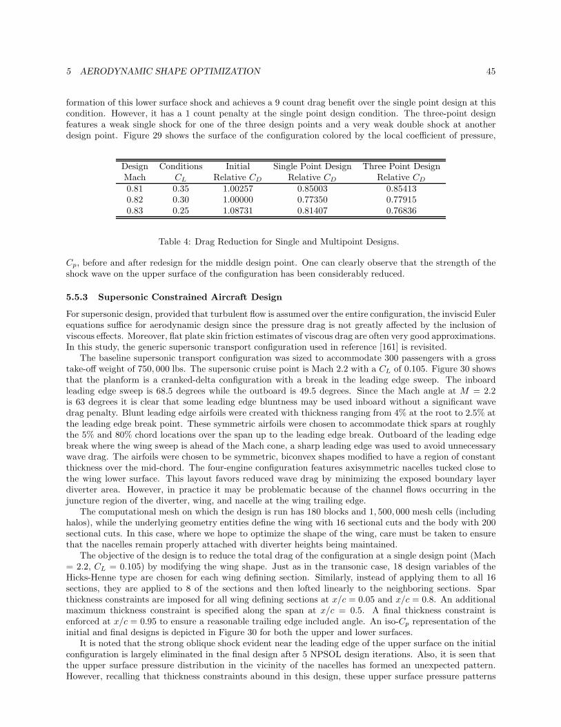
5 AERODYNAMIC SHAPE OPTIMIZATION 45

formation of this lower surface shock and achieves a 9 count drag benefit over the single point design at thiscondition. However, it has a 1 count penalty at the single point design condition. The three-point designfeatures a weak single shock for one of the three design points and a very weak double shock at anotherdesign point. Figure 29 shows the surface of the configuration colored by the local coefficient of pressure,

Design Conditions Initial Single Point Design Three Point DesignMach CL Relative CD Relative CD Relative CD

0.81 0.35 1.00257 0.85003 0.854130.82 0.30 1.00000 0.77350 0.779150.83 0.25 1.08731 0.81407 0.76836

Table 4: Drag Reduction for Single and Multipoint Designs.

Cp, before and after redesign for the middle design point. One can clearly observe that the strength of theshock wave on the upper surface of the configuration has been considerably reduced.

5.5.3 Supersonic Constrained Aircraft Design

For supersonic design, provided that turbulent flow is assumed over the entire configuration, the inviscid Eulerequations suffice for aerodynamic design since the pressure drag is not greatly affected by the inclusion ofviscous effects. Moreover, flat plate skin friction estimates of viscous drag are often very good approximations.In this study, the generic supersonic transport configuration used in reference [161] is revisited.

The baseline supersonic transport configuration was sized to accommodate 300 passengers with a grosstake-off weight of 750, 000 lbs. The supersonic cruise point is Mach 2.2 with a CL of 0.105. Figure 30 showsthat the planform is a cranked-delta configuration with a break in the leading edge sweep. The inboardleading edge sweep is 68.5 degrees while the outboard is 49.5 degrees. Since the Mach angle at M = 2.2is 63 degrees it is clear that some leading edge bluntness may be used inboard without a significant wavedrag penalty. Blunt leading edge airfoils were created with thickness ranging from 4% at the root to 2.5% atthe leading edge break point. These symmetric airfoils were chosen to accommodate thick spars at roughlythe 5% and 80% chord locations over the span up to the leading edge break. Outboard of the leading edgebreak where the wing sweep is ahead of the Mach cone, a sharp leading edge was used to avoid unnecessarywave drag. The airfoils were chosen to be symmetric, biconvex shapes modified to have a region of constantthickness over the mid-chord. The four-engine configuration features axisymmetric nacelles tucked close tothe wing lower surface. This layout favors reduced wave drag by minimizing the exposed boundary layerdiverter area. However, in practice it may be problematic because of the channel flows occurring in thejuncture region of the diverter, wing, and nacelle at the wing trailing edge.

The computational mesh on which the design is run has 180 blocks and 1, 500, 000 mesh cells (includinghalos), while the underlying geometry entities define the wing with 16 sectional cuts and the body with 200sectional cuts. In this case, where we hope to optimize the shape of the wing, care must be taken to ensurethat the nacelles remain properly attached with diverter heights being maintained.

The objective of the design is to reduce the total drag of the configuration at a single design point (Mach= 2.2, CL = 0.105) by modifying the wing shape. Just as in the transonic case, 18 design variables of theHicks-Henne type are chosen for each wing defining section. Similarly, instead of applying them to all 16sections, they are applied to 8 of the sections and then lofted linearly to the neighboring sections. Sparthickness constraints are imposed for all wing defining sections at x/c = 0.05 and x/c = 0.8. An additionalmaximum thickness constraint is specified along the span at x/c = 0.5. A final thickness constraint isenforced at x/c = 0.95 to ensure a reasonable trailing edge included angle. An iso-Cp representation of theinitial and final designs is depicted in Figure 30 for both the upper and lower surfaces.

It is noted that the strong oblique shock evident near the leading edge of the upper surface on the initialconfiguration is largely eliminated in the final design after 5 NPSOL design iterations. Also, it is seen thatthe upper surface pressure distribution in the vicinity of the nacelles has formed an unexpected pattern.However, recalling that thickness constraints abound in this design, these upper surface pressure patterns

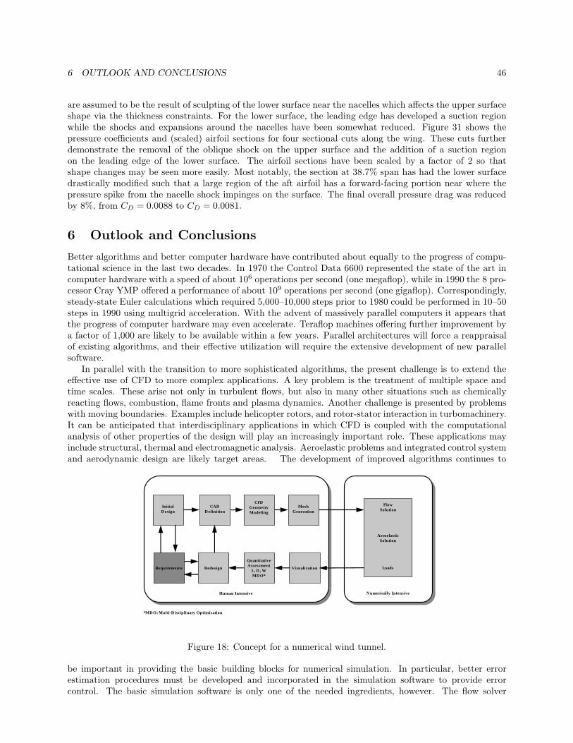
6 OUTLOOK AND CONCLUSIONS 46

are assumed to be the result of sculpting of the lower surface near the nacelles which affects the upper surfaceshape via the thickness constraints. For the lower surface, the leading edge has developed a suction regionwhile the shocks and expansions around the nacelles have been somewhat reduced. Figure 31 shows thepressure coefficients and (scaled) airfoil sections for four sectional cuts along the wing. These cuts furtherdemonstrate the removal of the oblique shock on the upper surface and the addition of a suction regionon the leading edge of the lower surface. The airfoil sections have been scaled by a factor of 2 so thatshape changes may be seen more easily. Most notably, the section at 38.7% span has had the lower surfacedrastically modified such that a large region of the aft airfoil has a forward-facing portion near where thepressure spike from the nacelle shock impinges on the surface. The final overall pressure drag was reducedby 8%, from CD = 0.0088 to CD = 0.0081.

6 Outlook and Conclusions

Better algorithms and better computer hardware have contributed about equally to the progress of compu-tational science in the last two decades. In 1970 the Control Data 6600 represented the state of the art incomputer hardware with a speed of about 106 operations per second (one megaflop), while in 1990 the 8 pro-cessor Cray YMP offered a performance of about 109 operations per second (one gigaflop). Correspondingly,steady-state Euler calculations which required 5,000–10,000 steps prior to 1980 could be performed in 10–50steps in 1990 using multigrid acceleration. With the advent of massively parallel computers it appears thatthe progress of computer hardware may even accelerate. Teraflop machines offering further improvement bya factor of 1,000 are likely to be available within a few years. Parallel architectures will force a reappraisalof existing algorithms, and their effective utilization will require the extensive development of new parallelsoftware.

In parallel with the transition to more sophisticated algorithms, the present challenge is to extend theeffective use of CFD to more complex applications. A key problem is the treatment of multiple space andtime scales. These arise not only in turbulent flows, but also in many other situations such as chemicallyreacting flows, combustion, flame fronts and plasma dynamics. Another challenge is presented by problemswith moving boundaries. Examples include helicopter rotors, and rotor-stator interaction in turbomachinery.It can be anticipated that interdisciplinary applications in which CFD is coupled with the computationalanalysis of other properties of the design will play an increasingly important role. These applications mayinclude structural, thermal and electromagnetic analysis. Aeroelastic problems and integrated control systemand aerodynamic design are likely target areas. The development of improved algorithms continues to

FlowSolution

AeroelasticSolution

Loads

Numerically IntensiveHuman Intensive

InitialDesign

CADDefinition

CFDGeometryModeling

MeshGeneration

Requirements Redesign

QuantitativeAssessment

L, D, WMDO*

Visualization

*MDO: Multi-Disciplinary Optimization

Figure 18: Concept for a numerical wind tunnel.

be important in providing the basic building blocks for numerical simulation. In particular, better errorestimation procedures must be developed and incorporated in the simulation software to provide errorcontrol. The basic simulation software is only one of the needed ingredients, however. The flow solver

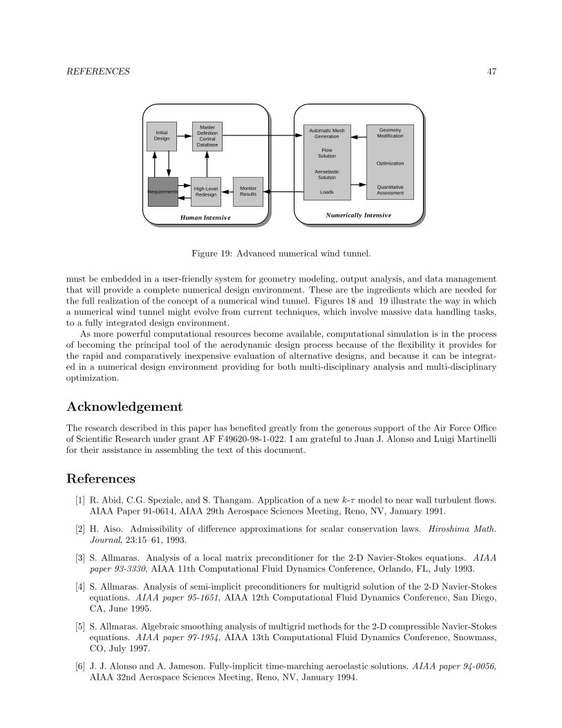
REFERENCES 47

Numerically IntensiveHuman Intensive

InitialDesign

MasterDefinitionCentral

Database

RequirementsHigh-LevelRedesign

GeometryModification

Optimization

QuantitativeAssessment

Automatic MeshGeneration

FlowSolution

Loads

AeroelasticSolution

MonitorResults

Figure 19: Advanced numerical wind tunnel.

must be embedded in a user-friendly system for geometry modeling, output analysis, and data managementthat will provide a complete numerical design environment. These are the ingredients which are needed forthe full realization of the concept of a numerical wind tunnel. Figures 18 and 19 illustrate the way in whicha numerical wind tunnel might evolve from current techniques, which involve massive data handling tasks,to a fully integrated design environment.

As more powerful computational resources become available, computational simulation is in the processof becoming the principal tool of the aerodynamic design process because of the flexibility it provides forthe rapid and comparatively inexpensive evaluation of alternative designs, and because it can be integrat-ed in a numerical design environment providing for both multi-disciplinary analysis and multi-disciplinaryoptimization.

Acknowledgement

The research described in this paper has benefited greatly from the generous support of the Air Force Officeof Scientific Research under grant AF F49620-98-1-022. I am grateful to Juan J. Alonso and Luigi Martinellifor their assistance in assembling the text of this document.

References

[1] R. Abid, C.G. Speziale, and S. Thangam. Application of a new k-τ model to near wall turbulent flows.AIAA Paper 91-0614, AIAA 29th Aerospace Sciences Meeting, Reno, NV, January 1991.

[2] H. Aiso. Admissibility of difference approximations for scalar conservation laws. Hiroshima Math.Journal, 23:15–61, 1993.

[3] S. Allmaras. Analysis of a local matrix preconditioner for the 2-D Navier-Stokes equations. AIAApaper 93-3330, AIAA 11th Computational Fluid Dynamics Conference, Orlando, FL, July 1993.

[4] S. Allmaras. Analysis of semi-implicit preconditioners for multigrid solution of the 2-D Navier-Stokesequations. AIAA paper 95-1651, AIAA 12th Computational Fluid Dynamics Conference, San Diego,CA, June 1995.

[5] S. Allmaras. Algebraic smoothing analysis of multigrid methods for the 2-D compressible Navier-Stokesequations. AIAA paper 97-1954, AIAA 13th Computational Fluid Dynamics Conference, Snowmass,CO, July 1997.

[6] J. J. Alonso and A. Jameson. Fully-implicit time-marching aeroelastic solutions. AIAA paper 94-0056,AIAA 32nd Aerospace Sciences Meeting, Reno, NV, January 1994.

REFERENCES 48

[7] J. J. Alonso, L. Martinelli, and A. Jameson. Multigrid unsteady Navier-Stokes calculations withaeroelastic applications. AIAA paper 95-0048, AIAA 33rd Aerospace Sciences Meeting, Reno, NV,January 1995.

[8] B.K. Anderson, J.L. Thomas, and B. Van Leer. A comparison of flux vector splittings for the Eulerequations. AIAA Paper 85-0122, AIAA 23rd Aerospace Sciences Meeting, Reno, NV, January 1985.

[9] W.K. Anderson, J.L. Thomas, and D.L. Whitfield. Multigrid acceleration of the flux split Eulerequations. AIAA Paper 86-0274, AIAA 24th Aerospace Sciences Meeting, Reno, NV, January 1986.

[10] W.K. Anderson and V. Venkatakrishnan. Aerodynamic design and optimization on unstructured gridswith a continuous adjoint formulation. AIAA paper 97-0643, AIAA 35th Aerospace Sciences Meeting,Reno, NV, January 1997.

[11] T.J. Baker. Mesh generation by a sequence of transformations. Appl. Num. Math., 2:515–528, 1986.

[12] N. Balakrishnan and S. M. Deshpande. New upwind schemes with wave-particle splitting for inviscidcompressible flows. Report 91 FM 12, Indian Institute of Science, 1991.

[13] B. Baldwin and H. Lomax. Thin layer approximation and algebraic model for separated turbulentflow. AIAA Paper 78-257, 1978.

[14] B.S. Baldwin and T.J. Barth. A one-equation turbulence transport model for high Reynolds numberwall-bounded flows. AIAA Paper 91-0610, AIAA 29th Aerospace Sciences Meeting, Reno, NV, January1991.

[15] T. J. Barth. Aspects of unstructured grids and finite volume solvers for the Euler and Navier Stokesequations. In von Karman Institute for Fluid Dynamics Lecture Series Notes 1994-05, Brussels, 1994.

[16] T.J. Barth and P.O. Frederickson. Higher order solution of the Euler equations on unstructured gridsusing quadratic reconstruction. AIAA paper 90-0013, AIAA 28th Aerospace Sciences Meeting, January1990.

[17] T.J. Barth and D.C. Jespersen. The design and application of upwind schemes on unstructured meshes.AIAA paper 89-0366, AIAA 27th Aerospace Sciences Meeting, Reno, NV, January 1989.

[18] J.T. Batina. Implicit flux-split Euler schemes for unsteady aerodynamic analysis involving unstructureddynamic meshes. AIAA paper 90-0936, April 1990.

[19] F. Bauer, P. Garabedian, D. Korn, and A. Jameson. Supercritical Wing Sections II. Springer Verlag,New York, 1975.

[20] O. Baysal and M. E. Eleshaky. Aerodynamic design optimization using sensitivity anaysis and compu-tational fluid dynamics. AIAA paper 91-0471, 29th Aerospace Sciences Meeting, Reno, NV, January1991.

[21] R.W. Beam and R.F. Warming. An implicit finite difference algorithm for hyperbolic systems inconservation form. J. Comp. Phys., 23:87–110, 1976.

[22] A. Belov, L. Martinelli, and A. Jameson. A new implicit algorithm with multigrid for unsteadyincompressible flow calculations. AIAA paper 95-0049, AIAA 33rd Aerospace Sciences Meeting, Reno,NV, January 1995.

[23] J.A. Benek, P.G. Buning, and J.L. Steger. A 3-D Chimera grid embedding technique. AIAA Paper85-1523, AIAA 7th Computational Fluid Dynamics Conference, Cincinnati, OH, 1985.

[24] J.A. Benek, T.L. Donegan, and N.E. Suhs. Extended Chimera grid embedding scheme with applica-tions to viscous flows. AIAA Paper 87-1126, AIAA 8th Computational Fluid Dynamics Conference,Honolulu, HI, 1987.

REFERENCES 49

[25] M. Berger and A. Jameson. Automatic adaptive grid refinement for the Euler equations. AIAA Journal,23:561–568, 1985.

[26] M. Berger and R.J. LeVeque. An adaptive Cartesian mesh algorithm for the Euler equations inarbitrary geometries. AIAA Paper 89-1930, 1989.

[27] J.P. Boris and D.L. Book. Flux corrected transport, 1 SHASTA, a fluid transport algorithm thatworks. J. Comp. Phys., 11:38–69, 1973.

[28] A. Brandt. Multi-level adaptive solutions to boundary value problems. Math. Comp., 31:333–390,1977.

[29] M.O. Bristeau, R. Glowinski, J. Periaux, P. Perrier, O. Pironneau, and C. Poirier. On the numericalsolution of nonlinear problems in fluid dynamics by least squares and finite element methods (II),application to transonic flow simulations. Comp. Meth. Appl. Mech. and Eng., 51:363–394, 1985.

[30] R.J. Busch, Jr. Computational fluid dynamics in the design of the Northrop/McDonnell DouglasYF-23 ATF prototype. AIAA paper 91-1627, AIAA 21st Fluid Dynamics, Plasmadynamics & LasersConference, Honolulu, Hawaii, 1991.

[31] H. Cabuk, C.H. Shung, and V. Modi. Adjoint operator approach to shape design for internal in-compressible flow. In G. S. Dulikravich, editor, Proceedings of the Third International Conference onInverse Design and Optimization in Engineering Sciences, pages 391–404, 1991.

[32] C. Canuto, M.Y. Hussaini, A. Quarteroni, and D.A. Zang. Spectral Methods in Fluid Dynamics.Springer Verlag, 1987.

[33] M.H. Carpenter, D. Gottlieb, and S. Abarbanel. Time-stable boundary conditions for finite-differenceschemes solving hyperbolic systems: Methodology and application to high-order compact schemes.ICASE Report 93-9, Hampton, VA, March 1993.

[34] D.A. Caughey. A diagonal implicit multigrid algorithm for the Euler equations. AIAA Paper 87-453,AIAA 25th Aerospace Sciences Meeting, Reno, NV, January 1987.

[35] T. Cebeci and A.M.O. Smith. Analysis of Turbulent Boundary Layers. Academic Press, 1974.

[36] S.R. Chakravarthy. Relaxation methods for unfactored implicit upwind schemes. AIAA Paper 84-0165,AIAA 22nd Aerospace Sciences Meeting, Reno, NV, January 1984.

[37] S.R. Chakravarthy, A. Harten, and S. Osher. Essentially non-oscillatory shock capturing schemes ofuniformly very high accuracy. AIAA Paper 86-0339, AIAA 24th Aerospace Sciences Meeting, Reno,NV, January 1986.

[38] R. Chipman and A. Jameson. Fully conservative numerical solutions for unsteady irrotational tran-sonic flow about airfoils. AIAA Paper 79-1555, AIAA 12th Fluid and Plasma Dynamics Conference,Williamsburg, VA, July 1979.

[39] S.E. Cliff and S.D. Thomas. Euler/experimental correlations of sonic boom pressure signatures. AIAAPaper 91-3276, AIAA 9th Applied Aerodynamics Conference, Baltimore, September 1991.

[40] T.J. Coakley. Numerical simulation of viscous transonic airfoil flows. AIAA Paper 87-0416, AIAA 25thAerospace Sciences Meeting, Reno, NV, January 1987.

[41] J.P. Croisille and P. Villedieu. Kinetic flux splitting schemes for hypersonic flows. In M. Napolitanoand F. Sobetta, editors, Proc 13th International Congress on Numerical Methods in Fluid Dynamics,pages 310–313, Rome, July 1992. Springer Verlag.

[42] P.I. Crumpton and M.B. Giles. Implicit time accurate solutions on unstructured dynamic grids. AIAApaper 95-1671, AIAA 12th Computational Fluid Dynamics Conference, San Diego, CA, June 1995.

REFERENCES 50

[43] R.M. Cummings, Y.M. Rizk, L.B. Schiff, and N.M. Chaderjian. Navier-Stokes predictions for the F-18wing and fuselage at large incidence. J. of Aircraft, 29:565–574, 1992.

[44] G. Dahlquist. A special stability problem for linear multistep methods. BIT, 3:27–43, 1963.

[45] J.F. Dannenhoffer and J.R. Baron. Robust grid adaptation for complex transonic flows. AIAA Paper86-0495, AIAA 24th Aerospace Sciences Meeting, Reno, NV, January 1986.

[46] H. Deconinck, H. Paillere, R. Struijs, and P.L. Roe. Multi-dimensional upwind schemes based onfluctuation-splitting of conservation laws. Comp. Mechanics, 11:323–340, 1993.

[47] D. Degani and L. Schiff. Computation of turbulent supersonic flows around pointed bodies havingcrossflow separation. J. Comp. Phys., 66:173–196, 1986.

[48] B. Delaunay. Sur la sphere vide. Bull. Acad. Science USSR VII: Class Scil, Mat. Nat., pages 793–800,1934.

[49] M. Desai and K. Ito. Optimal controls of Navier-Stokes equations. SIAM J. Control Optim., 32(5):1428–1446, 1994.

[50] S.M. Deshpande. On the Maxwellian distribution, symmetric form and entropy conservation for theEuler equations. NASA TP 2583, 1986.

[51] A. Eberle. A finite volume method for calculating transonic potential flow around wings from theminimum pressure integral. NASA TM 75324, 1978. Translated from MBB UFE 1407(0).

[52] P.R. Eiseman. A multi-surface method of coordinate generation. J. Comp. Phys., 33:118–150, 1979.

[53] J. Elliot and J. Peraire. Practical 3D aerodynamic design and optimization using unstructured mesh-es. AIAA paper 96-4710, 6th AIAA/NASA/USAF Multidisciplinary and Optimization Symposium,Seattle, WA, September 1996.

[54] W. Eppard and B. Grossman. A multi-dimensional kinetic-based upwind solver for the Euler equations.AIAA Paper 93-3303, AIAA 11th Computational Fluid Dynamics Conference, Orlando, FL, July 1993.

[55] L.E. Eriksson. Generation of boundary-conforming grids around wing-body configurations using trans-finite interpolation. AIAA Journal, 20:1313–1320, 1982.

[56] J. Farmer, L. Martinelli, A. Jameson, and G. Cowles. Fully-nonlinear CFD techniques for ship perfor-mance analysis and design. AIAA paper 95-1690, AIAA 12th Computational Fluid Dynamics Confer-ence, San Diego, CA, June 1995.

[57] R.P. Fedorenko. The speed of convergence of one iterative process. USSR Comp. Math. and Math.Phys., 4:227–235, 1964.

[58] J. Gallman, J. Reuther, N. Pfeiffer, W. Forrest, and D. Bernstorf. Business jet wing design usingaerodynamic shape optimization. AIAA paper 96-0554, 34th Aerospace Sciences Meeting and Exhibit,Reno, Nevada, January 1996.

[59] C.W. Gear. The numerical integration of stiff ordinary differential equations. Report 221, Universityof Illinois Department of Computer Science, 1967.

[60] M. Giles, M. Drela, and W.T. Thompkins. Newton solution of direct and inverse transonic Eulerequations. AIAA Paper 85-1530, Cincinnati, 1985.

[61] S.K. Godunov. A difference method for the numerical calculation of discontinuous solutions of hy-drodynamic equations. Mat. Sbornik, 47:271–306, 1959. Translated as JPRS 7225 by U.S. Dept. ofCommerce, 1960.

REFERENCES 51

[62] M.H. Ha. The impact of turbulence modelling on the numerical prediction of flows. In M. Napolitanoand F. Solbetta, editors, Proc. of the 13th International Conference on Numerical Methods in FluidDynamics, pages 27–46, Rome, Italy, July 1992. Springer Verlag, 1993.

[63] W. Hackbusch. On the multi-grid method applied to difference equations. Computing, 20:291–306,1978.

[64] M. Hafez, J.C. South, and E.M. Murman. Artificial compressibility method for numerical solutions ofthe transonic full potential equation. AIAA Journal, 17:838–844, 1979.

[65] M.G. Hall. Cell vertex multigrid schemes for solution of the Euler equations. In Proc. IMA Conferenceon Numerical Methods for Fluid Dynamics, Reading, April 1985.

[66] A. Harten. High resolution schemes for hyperbolic conservation laws. J. Comp. Phys., 49:357–393,1983.

[67] O. Hassan, K. Morgan, and J. Peraire. An adaptive implicit/explicit finite-element method for highspeed flows. AIAA paper 89-0363, AIAA 27th Aerospace Sciences Meeting, Reno, NV, January 1989.

[68] P.W. Hemker and S.P. Spekreijse. Multigrid solution of the steady Euler equations. In Proc. Oberwol-fach Meeting on Multigrid Methods, December 1984.

[69] J.L. Hess and A.M.O. Smith. Calculation of non-lifting potential flow about arbitrary three-dimensionalbodies. Douglas Aircraft Report ES 40622, 1962.

[70] C. Hirsch, C. Lacol, and H. Deconinck. Convection algorithms based on a diagonalization procedurefor the multi-dimensional Euler equations. AIAA Paper 87-1163, AIAA 8th Computational FluidDynamics Conference, Hawaii, June 1987.

[71] C. Hirsch and P. Van Ransbeeck. Multi-dimensional upwinding and artificial dissipation. Technicalreport. Published in Frontiers of Computational Fluid Dynamics 1994, D. A. Caughey and M. M.Hafez, editors, Wiley, pp. 597–626.

[72] D.G. Holmes and S.H. Lamson. Adaptive triangular meshes for compressible flow solutions. In Proceed-ings First International Conference on Numerical Grid Generation in Computational Fluid Dynamics,pages 413–424, Landshut, FRG, July 1986.

[73] J.C. Huan and V. Modi. Optimum design for drag minimizing bodies in incompressible flow. InverseProblems in Engineering, 1:1–25, 1994.

[74] T.J.R. Hughes, L.P. Franca, and M. Mallet. A new finite element formulation for computational fluiddynamics,I, Symmetric forms of the compressible Euler and Navier-Stokes equations and the secondlaw of thermodynamics. Comp. Meth. Appl. Mech. and Eng., 59:223–231, 1986.

[75] A. Jameson. Optimum aerodynamic design via boundary control. AGARD FDP/Von Karman InstituteLecture Notes on Optimum Design Methods in Aerodynamics. AGARD Report 803, pages 3-1 to 3-33,1994.

[76] A. Jameson. Iterative solution of transonic flows over airfoils and wings, including flows at Mach 1.Comm. on Pure and Appl. Math., 27:283–309, 1974.

[77] A. Jameson. Transonic potential flow calculations in conservation form. In Proc. AIAA 2nd Compu-tational Fluid Dynamics Conference, pages 148–161, Hartford, 1975.

[78] A. Jameson. Solution of the Euler equations by a multigrid method. Appl. Math. and Comp., 13:327–356, 1983.

[79] A. Jameson. Multigrid algorithms for compressible flow calculations. In Second European Conferenceon Multigrid Methods, Cologne, October 1985. Princeton University Report MAE 1743.

REFERENCES 52

[80] A. Jameson. Non-oscillatory shock capturing scheme using flux limited dissipation. In B.E. Engquist,S. Osher, and R.C.J. Sommerville, editors, Lectures in Applied Mathematics, Vol. 22, Part 1, LargeScale Computations in Fluid Mechanics, pages 345–370. AMS, 1985.

[81] A. Jameson. Transonic flow calculations for aircraft. In F. Brezzi, editor, Lecture Notes in Mathematics,Numerical Methods in Fluid Dynamics, pages 156–242. Springer Verlag, 1985.

[82] A. Jameson. A vertex based multigrid algorithm for three-dimensional compressible flow calculation-s. In T.E. Tezduar and T.J.R. Hughes, editors, Numerical Methods for Compressible Flow - FiniteDifference, Element And Volume Techniques, 1986. ASME Publication AMD 78.

[83] A. Jameson. Aerodynamic design via control theory. J. Sci. Comp., 3:233–260, 1988.

[84] A. Jameson. Automatic design of transonic airfoils to reduce the shock induced pressure drag. InProceedings of the 31st Israel Annual Conference on Aviation and Aeronautics, pages 5–17, Tel Aviv,February 1990.

[85] A. Jameson. Time dependent calculations using multigrid, with applications to unsteady flows pastairfoils and wings. AIAA paper 91-1596, AIAA 10th Computational Fluid Dynamics Conference,Honolulu, Hawaii, June 1991.

[86] A. Jameson. Artificial diffusion, upwind biasing, limiters and their effect on accuracy and multigridconvergence in transonic and hypersonic flows. AIAA paper 93-3359, AIAA 11th Computational FluidDynamics Conference, Orlando, FL, July 1993.

[87] A. Jameson. Analysis and design of numerical schemes for gas dynamics 1, artificial diffusion, upwindbiasing, limiters and their effect on multigrid convergence. Int. J. of Comp. Fluid Dyn., 4:171–218,1995.

[88] A. Jameson. Analysis and design of numerical schemes for gas dynamics 2, artificial diffusion anddiscrete shock structure. Int. J. of Comp. Fluid Dyn., 5:1–38, 1995.

[89] A. Jameson. Optimum aerodynamic design using the Control Theory. Computational Fluid DynamicsReview, pages 495–528, 1995.

[90] A. Jameson, J. J. Alonso, J. Reuther, L. Martinelli, and J. C. Vassberg. Aerodynamic shape optimiza-tion techniques based on control theory. AIAA paper 98-2538, AIAA 29th Fluid Dynamics Conference,Albuquerque, NM, June 1998.

[91] A. Jameson and T.J. Baker. Improvements to the aircraft Euler method. AIAA Paper 87-0452, AIAA25th Aerospace Sciences Meeting, Reno, NV, January 1987.

[92] A. Jameson, T.J. Baker, and N.P. Weatherill. Calculation of inviscid transonic flow over a completeaircraft. AIAA Paper 86-0103, AIAA 24th Aerospace Sciences Meeting, Reno, NV, January 1986.

[93] A. Jameson, L. Martinelli, and N. A. Pierce. Optimum aerodynamic design using the Navier-Stokesequations. Theoretical and Computational Fluid Dynamics, 10:213–237, 1998.

[94] A. Jameson and D.J. Mavriplis. Multigrid solution of the Euler equations on unstructured and adaptivegrids. In S. McCormick, editor, Multigrid Methods, Theory, Applications and Supercomputing. LectureNotes in Pure and Applied Mathematics, volume 110, pages 413–430, April 1987.

[95] A. Jameson, W. Schmidt, and E. Turkel. Numerical solution of the Euler equations by finite volumemethods using Runge-Kutta time stepping schemes. AIAA Paper 81-1259, June 1981.

[96] A. Jameson and E. Turkel. Implicit schemes and LU decompositions. Math. Comp., 37:385–397, 1981.

[97] M. Jayaram and A. Jameson. Multigrid solution of the Navier-Stokes equations for flow over wings.AIAA paper 88-0705, AIAA 26th Aerospace Sciences Meeting, Reno, NV, January 1988.

REFERENCES 53

[98] D. Johnson and L. King. A mathematically simple turbulence closure model for attached and separatedturbulent boundary layers. AIAA Journal, 23:1684–1692, 1985.

[99] W.P. Jones and B.E. Launder. The calculation of low-Reynolds-number phenomena with a two-equation model of turbulence. Int. J. of Heat Tran., 16:1119–1130, 1973.

[100] W.H. Jou. Boeing Memorandum AERO-B113B-L92-018, September 1992. To Joseph Shang.

[101] T.J. Kao, T.Y. Su, and N.J. Yu. Navier-Stokes calculations for transport wing-body configurationswith nacelles and struts. AIAA Paper 93-2945, AIAA 24th Fluid Dynamics Conference, Orlando, July1993.

[102] G.E. Karniadakis and S.A. Orszag. Nodes, modes and flow codes. Physics Today, pages 34–42, March1993.

[103] M.H. Lallemand and A. Dervieux. A multigrid finite-element method for solving the two-dimensionalEuler equations. In S.F. McCormick, editor, Proceedings of the Third Copper Mountain Conference onMultigrid Methods, Lecture Notes in Pure and Applied Mathematics, pages 337–363, Copper Mountain,April 1987.

[104] M.H. Lallemand, H. Steve, and A. Dervieux. Unstructured multigridding by volume aggregation:Current status. Computers and Fluids, 21:397–433, 1992.

[105] A.M. Landsberg, J.P. Boris, W. Sandberg, and T.R. Young. Naval ship superstructure design: Complexthree-dimensional flows using an efficient, parallel method. High Performance Computing 1993: GrandChallenges in Computer Simulation, 1993.

[106] P. D. Lax. Hyperbolic systems of conservation laws. SIAM Regional Series on Appl. Math., II, 1973.

[107] P.D. Lax. Hyperbolic systems of conservation laws and the mathematical theory of shock waves. SIAMRegional Series on Appl. Math., 11, 1973.

[108] P.D. Lax and B. Wendroff. Systems of conservation laws. Comm. Pure. Appl. Math., 13:217–237, l960.

[109] B. Van Leer. Towards the ultimate conservative difference scheme. II. Monotonicity and conservationcombined in a second order scheme. J. Comp. Phys., 14:361–370, 1974.

[110] B. Van Leer. Flux vector splitting for the Euler equations. In E. Krause, editor, Proceedings of the 8thInternational Conference on Numerical Methods in Fluid Dynamics, pages 507–512, Aachen, 1982.

[111] B. Van Leer. Progress in multi-dimensional upwind differencing. In M. Napolitano and F. Solbetta,editors, Proc. 13th International Conference on Numerical Methods in Fluid Dynamics, pages 1–26,Rome, July 1992. Springer Verlag, 1993.

[112] B. Van Leer, W. T. Lee, and P. L. Roe. Characteristic time stepping or local preconditioning ofthe Euler equations. AIAA paper 91-1552, AIAA 10th Computational Fluid Dynamics Conference,Honolulu, Hawaii, June 1991.

[113] D. Lefebre, J.Peraire, and K.Morgan. Finite element least squares solutions of the Euler equationsusing linear and quadratic approximations. Int. J. Comp. Fluid Dynamics, 1:1–23, 1993.

[114] S.K. Lele. Compact finite difference schemes with spectral-like resolution. CTR Manuscript 107, 1990.

[115] J.L. Lions. Optimal Control of Systems Governed by Partial Differential Equations. Springer-Verlag,New York, 1971. Translated by S.K. Mitter.

[116] M-S. Liou and C.J. Steffen. A new flux splitting scheme. J. Comp. Phys., 107:23–39, 1993.

[117] F. Liu and A. Jameson. Multigrid Navier-Stokes calculations for three-dimensional cascades. AIAApaper 92-0190, AIAA 30th Aerospace Sciences Meeting, Reno, NV, January 1992.

REFERENCES 54

[118] R. Lohner and D. Martin. An implicit linelet-based solver for incompressible flows. AIAA paper92-0668, AIAA 30th Aerospace Sciences Meeting, Reno, NV, January 1992.

[119] R. Lohner, K. Morgan, and J. Peraire. Improved adaptive refinement strategies for the finite elementaerodynamic configurations. AIAA Paper 86-0499, AIAA 24th Aerospace Sciences Meeting, Reno, NV,January 1986.

[120] R. Lohner, K. Morgan, J. Peraire, and O.C. Zienkiewicz. Finite element methods for high speed flows.AIAA Paper 85-1531, AIAA 7th Computational Fluid Dynamics Conference, Cincinnati, OH, 1985.

[121] R. Lohner and P. Parikh. Generation of three-dimensional unstructured grids by the advancing frontmethod. AIAA Paper 88-0515, Reno, NV, January 1988.

[122] R.W. MacCormack and A.J. Paullay. Computational efficiency achieved by time splitting of finitedifference operators. AIAA Paper 72-154, 1972.

[123] A. Majda and S. Osher. Numerical viscosity and the entropy condition. Comm. on Pure Appl. Math.,32:797–838, 1979.

[124] L. Martinelli and A. Jameson. Validation of a multigrid method for the Reynolds averaged equations.AIAA paper 88-0414, 1988.

[125] L. Martinelli, A. Jameson, and E. Malfa. Numerical simulation of three-dimensional vortex flowsover delta wing configurations. In M. Napolitano and F. Solbetta, editors, Proc. 13th InternationalConfrence on Numerical Methods in Fluid Dynamics, pages 534–538, Rome, Italy, July 1992. SpringerVerlag, 1993.

[126] L. Martinelli and V. Yakhot. RNG-based turbulence transport approximations with applications totransonic flows. AIAA Paper 89-1950, AIAA 9th Computational Fluid Dynamics Conference, Buffalo,NY, June 1989.

[127] D.J. Mavriplis. Multigrid strategies for viscous flow solvers on anisotropic unstructured meshes. AIAApaper 97-1952, AIAA 13th Computational Fluid Dynamics Conference, Snowmass, CO, July 1997.

[128] D.J. Mavriplis and A. Jameson. Multigrid solution of the Navier-Stokes equations on triangular meshes.AIAA Journal, 28(8):1415–1425, August 1990.

[129] D.J. Mavriplis and L. Martinelli. Multigrid solution of compressible turbulent flow on unstructuredmeshes using a two-equation model. AIAA Paper 91-0237, AIAA 29th Aerospace Sciences Meeting,Reno, NV, January 1991.

[130] D.J. Mavriplis and V. Venkatakrishnan. A 3D agglomeration multigrid solver for the Reynolds-averagedNavier-Stokes equations on unstructured meshes. Int. J. Numerical Methods in Fluids, 23:1–18, 1996.

[131] N. D. Melson, M. D. Sanetrik, and H. L. Atkins. Time-accurate Navier-Stokes calculations withmultigrid acceleration. In Proceedings of the Sixth Copper Mountain Conference on Multigrid Methods,Copper Mountain, April 1993.

[132] J.E. Melton, S.A. Pandya, and J.L. Steger. 3D Euler flow solutions using unstructured Cartesian andprismatic grids. AIAA Paper 93-0331, Reno, NV, January 1993.

[133] F. Menter. Zonal two-equation k-ω turbulence models for aerodynamic flows. AIAA Paper 93-2906,AIAA 24th Fluid Dynamics Meeting, Orlando, July 1993.

[134] W.A. Mulder. A new multigrid approach to convection problems. J. Comp. Phys., 83:303–323, 1989.

[135] W.A. Mulder. A high-resolution Euler solver based on multigrid, semi-coarsening, and defect correction.J. Comp. Phys., 100:91–104, 1992.

REFERENCES 55

[136] E.M. Murman. Analysis of embedded shock waves calculated by relaxation methods. AIAA Journal,12:626–633, 1974.

[137] E.M. Murman and J.D. Cole. Calculation of plane steady transonic flows. AIAA Journal, 9:114–121,1971.

[138] R.H. Ni. A multiple grid scheme for solving the Euler equations. AIAA Journal, 20:1565–1571, 1982.

[139] S. Obayashi and K. Kuwakara. LU factorization of an implicit scheme for the compressible Navier-Stokes equations. AIAA Paper 84-1670, AIAA 17th Fluid Dynamics and Plasma Dynamics Conference,Snowmass, CO, June 1984.

[140] J.T. Oden, L. Demkowicz, T. Liszka, and W. Rachowicz. h-p adaptive finite element methods for com-pressible and incompressible flows. In S. L. Venneri A. K. Noor, editor, Proceedings of the Symposiumon Computational Technology on Flight Vehicles, pages 523–534, Washington, D.C., November 1990.Pergamon.

[141] S. Orszag and D. Gottlieb. Numerical analysis of spectral methods. SIAM Regional Series on Appl.Math., 26, 1977.

[142] S. Osher. Riemann solvers, the entropy condition, and difference approximations. SIAM J. Num.Anal., 121:217–235, 1984.

[143] S. Osher and S. Chakravarthy. High resolution schemes and the entropy condition. SIAM J. NumAnal., 21:955–984, 1984.

[144] S. Osher and F. Solomon. Upwind difference schemes for hyperbolic systems of conservation laws.Math. Comp., 38:339–374, 1982.

[145] S. Osher and E. Tadmor. On the convergence of difference approximations to scalar conservation laws.Math. Comp., 50:19–51, 1988.

[146] H. Paillere and H. Deconinck. A review of multi-dimensional upwind residual distribution schemes forthe euler equations. In M. Hafez and K. Oshima, editors, Computational Fluid Dynamics Review 1995,pages 141–160. Wiley, 1995.

[147] V. Parthasarathy, Y. Kallinderis, and K. Nakajima. A hybrid adaptation method and directionalviscous multigrid with prismatic-tetrahedral meshes. AIAA paper 95-0670, AIAA 33rd AerospaceSciences Meeting, Reno, Nevada, January 1995.

[148] J. Peraire, J. Peiro, and K. Morgan. A 3D finite-element multigrid solver for the Euler equations.AIAA paper 92-0449, AIAA 30th Aerospace Sciences Conference, Reno, NV, January 1992.

[149] J. Peraire, J. Peiro, and K. Morgan. Adaptive remeshing for three-dimensional compressible flowcomputations. J. Comp. Phys., 103(2):269–285, 1992.

[150] N.A. Pierce and M.B. Giles. Preconditioning compressible flow calculations on stretched meshes. AIAAPaper 96-0889, AIAA 34th Aerospace Sciences Meeting, Reno, NV, January 1996.

[151] N.A. Pierce, M.B. Giles, A. Jameson, and L. Martinelli. Accelerating three-dimensional Navier-Stokescalculations. AIAA Paper 97-1953, AIAA 13th Computational Fluid Dynamics Conference, Snowmass,CO, July 1997.

[152] O. Pironneau. Optimal shape design for aerodynamics. AGARD FDP/Von Karman Institute LectureNotes on Optimum Design Methods in Aerodynamics. AGARD Report 803, pages 6-1 to 6-40, 1994.

[153] O. Pironneau. Optimal Shape Design for Elliptic Systems. Springer-Verlag, New York, 1984.

[154] K.G. Powell and B. van Leer. A genuinely multidimensional upwind cell-vertex scheme for the Eulerequations. AIAA Paper 89-0095, AIAA 27th Aerospace Sciences Meeting, Reno, NV, January 1989.

REFERENCES 56

[155] K. Prendergast and K. Xu. Numerical hydrodynamics from gas kinetic theory. J. Comp. Phys.,109:53–66, November 1993.

[156] T.H. Pulliam and J.L. Steger. Implicit finite difference simulations of three-dimensional compressibleflow. AIAA Journal, 18:159–167, 1980.

[157] J.J. Quirk. An alternative to unstructured grids for computing gas dynamics flows about arbitrarilycomplex two-dimensional bodies. ICASE Report 92-7, Hampton, VA, February 1992.

[158] R. Radespiel, C. Rossow, and R.C. Swanson. An efficient cell-vertex multigrid scheme for the three-dimensional Navier-Stokes equations. In Proc. AIAA 9th Computational Fluid Dynamics Conference,pages 249–260, Buffalo, NY, June 1989. AIAA Paper 89-1953-CP.

[159] M.M. Rai and P. Moin. Direct numerical simulation of transition and turbulence in a spatially evolvingboundary layer. AIAA Paper 91-1607 CP, AIAA 10th Computational Fluid Dynamics Conference,Honolulu, HI, June 1991.

[160] S. V. Rao and S. M. Deshpande. A class of efficient kinetic upwind methods for compressible flows.Report 91 FM 11, Indian Institute of Science, 1991.

[161] J. Reuther, J.J. Alonso, M.J. Rimlinger, and A. Jameson. Aerodynamic shape optimization of super-sonic aircraft configurations via an adjoint formulation on parallel computers. AIAA paper 96-4045,6th AIAA/NASA/ISSMO Symposium on Multidisciplinary Analysis and Optimization, Bellevue, WA,September 1996.

[162] J. Reuther and A. Jameson. Aerodynamic shape optimization of wing and wing-body configurationsusing control theory. AIAA paper 95-0213, AIAA 33rd Aerospace Sciences Meeting and Exibit, Reno,NV, January 1995.

[163] H. Rieger and A. Jameson. Solution of steady three-dimensional compressible Euler and Navier-Stokesequations by and implicit LU scheme. AIAA paper 88-0619, AIAA 26th Aerospace Sciences Meeting,Reno, NV, January 1988.

[164] A. Rizzi and L.E. Eriksson. Computation of flow around wings based on the Euler equations. J. FluidMech., 148:45–71, 1984.

[165] T.W. Roberts and D. Sidilkover R.C. Swanson. Textbook multigrid efficiency for the steady eulerequations. AIAA paper 97-1949, AIAA 13th Computational Fluid Dynamics Conference, Snowmass,CO, July 1997.

[166] P.L. Roe. Approximate Riemann solvers, parameter vectors, and difference schemes. J. Comp. Phys.,43:357–372, 1981.

[167] P.E. Rubbert and G.R. Saaris. A general three-dimensional potential flow method applied to V/STOLaerodynamics. SAE Paper 680304, 1968.

[168] C.L. Rumsey and V.N. Vatsa. A comparison of the predictive capabilities of several turbulence modelsusing upwind and centered - difference computer codes. AIAA Paper 93-0192, AIAA 31st AerospaceSciences Meeting, Reno, NV, January 1993.

[169] S.S. Samant, J.E. Bussoletti, F.T. Johnson, R.H. Burkhart, B.L. Everson, R.G. Melvin, D.P. Young,L.L. Erickson, and M.D. Madson. TRANAIR: A computer code for transonic analyses of arbitraryconfigurations. AIAA Paper 87-0034, 1987.

[170] K. Sawada and S. Takanashi. A numerical investigation on wing/nacelle interferences of USB config-uration. AIAA paper 87-0455, AIAA 25th Aerospace Sciences Meeting, Reno, NV, January 1987.

[171] C.W. Shu and S. Osher. Efficient implementation of essentially non-oscillatory shock-capturingschemes. J. Comp. Phys., 77:439–471, 1988.

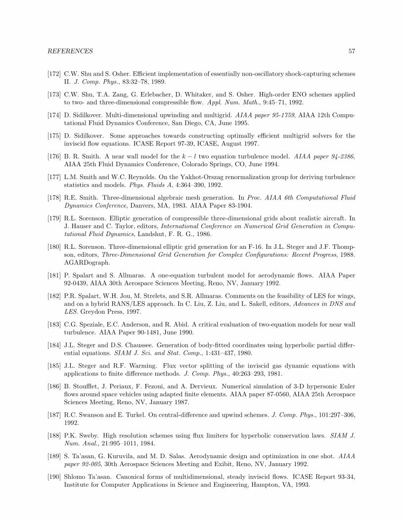
REFERENCES 57

[172] C.W. Shu and S. Osher. Efficient implementation of essentially non-oscillatory shock-capturing schemesII. J. Comp. Phys., 83:32–78, 1989.

[173] C.W. Shu, T.A. Zang, G. Erlebacher, D. Whitaker, and S. Osher. High-order ENO schemes appliedto two- and three-dimensional compressible flow. Appl. Num. Math., 9:45–71, 1992.

[174] D. Sidilkover. Multi-dimensional upwinding and multigrid. AIAA paper 95-1759, AIAA 12th Compu-tational Fluid Dynamics Conference, San Diego, CA, June 1995.

[175] D. Sidilkover. Some approaches towards constructing optimally efficient multigrid solvers for theinviscid flow equations. ICASE Report 97-39, ICASE, August 1997.

[176] B. R. Smith. A near wall model for the k − l two equation turbulence model. AIAA paper 94-2386,AIAA 25th Fluid Dynamics Conference, Colorado Springs, CO, June 1994.

[177] L.M. Smith and W.C. Reynolds. On the Yakhot-Orszag renormalization group for deriving turbulencestatistics and models. Phys. Fluids A, 4:364–390, 1992.

[178] R.E. Smith. Three-dimensional algebraic mesh generation. In Proc. AIAA 6th Computational FluidDynamics Conference, Danvers, MA, 1983. AIAA Paper 83-1904.

[179] R.L. Sorenson. Elliptic generation of compressible three-dimensional grids about realistic aircraft. InJ. Hauser and C. Taylor, editors, International Conference on Numerical Grid Generation in Compu-tational Fluid Dynamics, Landshut, F. R. G., 1986.

[180] R.L. Sorenson. Three-dimensional elliptic grid generation for an F-16. In J.L. Steger and J.F. Thomp-son, editors, Three-Dimensional Grid Generation for Complex Configurations: Recent Progress, 1988.AGARDograph.

[181] P. Spalart and S. Allmaras. A one-equation turbulent model for aerodynamic flows. AIAA Paper92-0439, AIAA 30th Aerospace Sciences Meeting, Reno, NV, January 1992.

[182] P.R. Spalart, W.H. Jou, M. Strelets, and S.R. Allmaras. Comments on the feasibility of LES for wings,and on a hybrid RANS/LES approach. In C. Liu, Z. Liu, and L. Sakell, editors, Advances in DNS andLES. Greydon Press, 1997.

[183] C.G. Speziale, E.C. Anderson, and R. Abid. A critical evaluation of two-equation models for near wallturbulence. AIAA Paper 90-1481, June 1990.

[184] J.L. Steger and D.S. Chaussee. Generation of body-fitted coordinates using hyperbolic partial differ-ential equations. SIAM J. Sci. and Stat. Comp., 1:431–437, 1980.

[185] J.L. Steger and R.F. Warming. Flux vector splitting of the inviscid gas dynamic equations withapplications to finite difference methods. J. Comp. Phys., 40:263–293, 1981.

[186] B. Stoufflet, J. Periaux, F. Fezoui, and A. Dervieux. Numerical simulation of 3-D hypersonic Eulerflows around space vehicles using adapted finite elements. AIAA paper 87-0560, AIAA 25th AerospaceSciences Meeting, Reno, NV, January 1987.

[187] R.C. Swanson and E. Turkel. On central-difference and upwind schemes. J. Comp. Phys., 101:297–306,1992.

[188] P.K. Sweby. High resolution schemes using flux limiters for hyperbolic conservation laws. SIAM J.Num. Anal., 21:995–1011, 1984.

[189] S. Ta’asan, G. Kuruvila, and M. D. Salas. Aerodynamic design and optimization in one shot. AIAApaper 92-005, 30th Aerospace Sciences Meeting and Exibit, Reno, NV, January 1992.

[190] Shlomo Ta’asan. Canonical forms of multidimensional, steady inviscid flows. ICASE Report 93-34,Institute for Computer Applications in Science and Engineering, Hampton, VA, 1993.

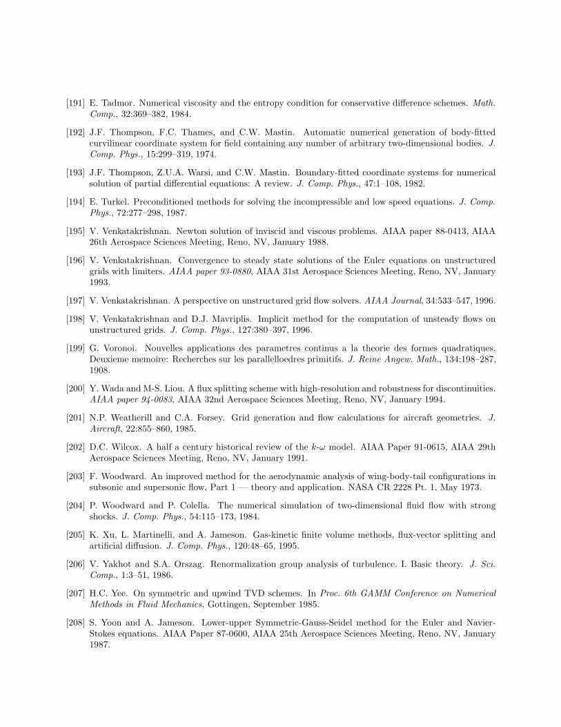
[191] E. Tadmor. Numerical viscosity and the entropy condition for conservative difference schemes. Math.Comp., 32:369–382, 1984.

[192] J.F. Thompson, F.C. Thames, and C.W. Mastin. Automatic numerical generation of body-fittedcurvilinear coordinate system for field containing any number of arbitrary two-dimensional bodies. J.Comp. Phys., 15:299–319, 1974.

[193] J.F. Thompson, Z.U.A. Warsi, and C.W. Mastin. Boundary-fitted coordinate systems for numericalsolution of partial differential equations: A review. J. Comp. Phys., 47:1–108, 1982.

[194] E. Turkel. Preconditioned methods for solving the incompressible and low speed equations. J. Comp.Phys., 72:277–298, 1987.

[195] V. Venkatakrishnan. Newton solution of inviscid and viscous problems. AIAA paper 88-0413, AIAA26th Aerospace Sciences Meeting, Reno, NV, January 1988.

[196] V. Venkatakrishnan. Convergence to steady state solutions of the Euler equations on unstructuredgrids with limiters. AIAA paper 93-0880, AIAA 31st Aerospace Sciences Meeting, Reno, NV, January1993.

[197] V. Venkatakrishnan. A perspective on unstructured grid flow solvers. AIAA Journal, 34:533–547, 1996.

[198] V. Venkatakrishnan and D.J. Mavriplis. Implicit method for the computation of unsteady flows onunstructured grids. J. Comp. Phys., 127:380–397, 1996.

[199] G. Voronoi. Nouvelles applications des parametres continus a la theorie des formes quadratiques.Deuxieme memoire: Recherches sur les parallelloedres primitifs. J. Reine Angew. Math., 134:198–287,1908.

[200] Y. Wada and M-S. Liou. A flux splitting scheme with high-resolution and robustness for discontinuities.AIAA paper 94-0083, AIAA 32nd Aerospace Sciences Meeting, Reno, NV, January 1994.

[201] N.P. Weatherill and C.A. Forsey. Grid generation and flow calculations for aircraft geometries. J.Aircraft, 22:855–860, 1985.

[202] D.C. Wilcox. A half a century historical review of the k-ω model. AIAA Paper 91-0615, AIAA 29thAerospace Sciences Meeting, Reno, NV, January 1991.

[203] F. Woodward. An improved method for the aerodynamic analysis of wing-body-tail configurations insubsonic and supersonic flow, Part 1 — theory and application. NASA CR 2228 Pt. 1, May 1973.

[204] P. Woodward and P. Colella. The numerical simulation of two-dimensional fluid flow with strongshocks. J. Comp. Phys., 54:115–173, 1984.

[205] K. Xu, L. Martinelli, and A. Jameson. Gas-kinetic finite volume methods, flux-vector splitting andartificial diffusion. J. Comp. Phys., 120:48–65, 1995.

[206] V. Yakhot and S.A. Orszag. Renormalization group analysis of turbulence. I. Basic theory. J. Sci.Comp., 1:3–51, 1986.

[207] H.C. Yee. On symmetric and upwind TVD schemes. In Proc. 6th GAMM Conference on NumericalMethods in Fluid Mechanics, Gottingen, September 1985.

[208] S. Yoon and A. Jameson. Lower-upper Symmetric-Gauss-Seidel method for the Euler and Navier-Stokes equations. AIAA Paper 87-0600, AIAA 25th Aerospace Sciences Meeting, Reno, NV, January1987.

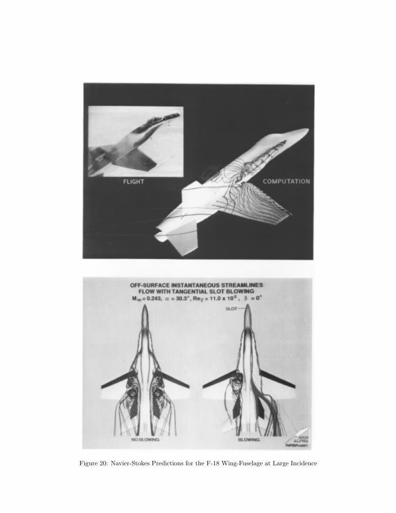
Figure 20: Navier-Stokes Predictions for the F-18 Wing-Fuselage at Large Incidence

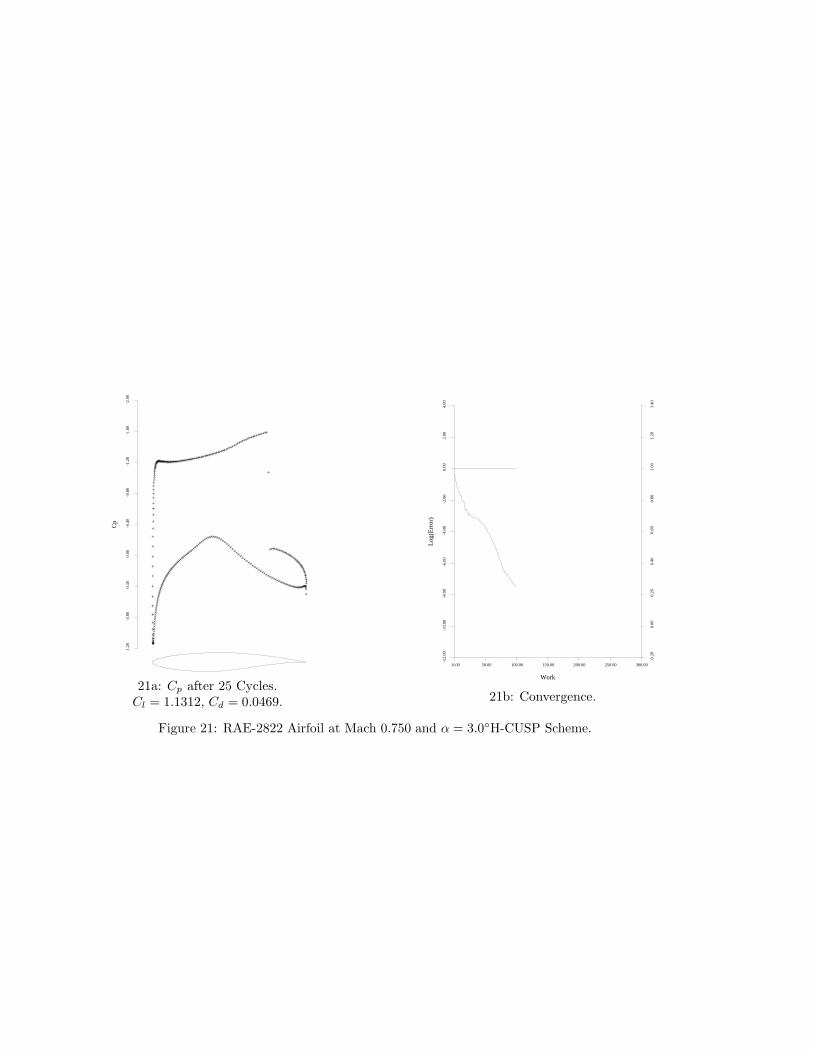
1.

20

0.80

0.

40

0.00

-0.

40 -

0.80

-1.

20 -

1.60

-2.

00

Cp

+++++++++++++++++++++

++++++++++

+++++++

++++++

++++

++++

++++

++++++++++++++++++++++++++++++++++++++++++++++++++++++++++++++++++++++++++++++++++++

++++++

+

+

+

+

+

+

+

+

+++++++++++++++++++++++++++++++++++++++++++++++++++++++++++++++++++++++++++++

++++++++++++++++++++

+++++++++++

++++++++

+++++++++++

++

+

+++++++++++++++++++++++++++++++++++++

21a: Cp after 25 Cycles.Cl = 1.1312, Cd = 0.0469.

0.00 50.00 100.00 150.00 200.00 250.00 300.00

Work

-12

.00

-10

.00

-8.

00 -

6.00

-4.

00 -

2.00

0.

00

2.00

4.

00

Log

(Err

or)

-0.

20

0.00

0.

20

0.40

0.

60

0.80

1.

00

1.20

1.

40

21b: Convergence.

Figure 21: RAE-2822 Airfoil at Mach 0.750 and α = 3.0H-CUSP Scheme.

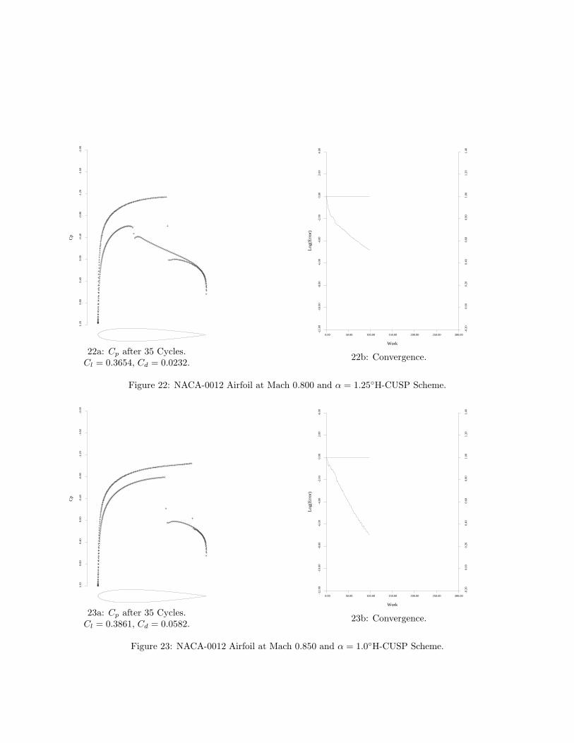
1.

20

0.80

0.

40

0.00

-0.

40 -

0.80

-1.

20 -

1.60

-2.

00

Cp

++++++++++++

++++++

++++++++

++++++++

++++++++

++++++++

++++++++

++++++++

++++++++

+++++++++++++++++++++++++++++++++++++++++++++++++++++++++++++++++++++++++++++++++++++++

++++++++++++++++++++++++++++++++++++++++++++++++++++++++

++++++++

++++++++++

+++++++++++++

+++++++++++++++++++++++++

++

+

+++++++++++++++++++++++++++++++++++++++++++++

22a: Cp after 35 Cycles.Cl = 0.3654, Cd = 0.0232.

0.00 50.00 100.00 150.00 200.00 250.00 300.00

Work

-12

.00

-10

.00

-8.

00 -

6.00

-4.

00 -

2.00

0.

00

2.00

4.

00

Log

(Err

or)

-0.

20

0.00

0.

20

0.40

0.

60

0.80

1.

00

1.20

1.

40

22b: Convergence.

Figure 22: NACA-0012 Airfoil at Mach 0.800 and α = 1.25H-CUSP Scheme.

1.

20

0.80

0.

40

0.00

-0.

40 -

0.80

-1.

20 -

1.60

-2.

00

Cp

++++++++++++

+++++++

+++++++++

++++++++++++++++++

+

+++++++++++++++++++++++++++++++++++++++++++++++++++++++++++++++++++++++++++++++++++++++++++++++++++++++++++++++++++

+++++++++++++++++++++++++++++++++++++++++++++++++++++++++

++++++++

++++++++++

+++++++++++++

++++++++++++++++++++

++++++++++++++++++++++++++

+

++++++++++++++++++++++++

23a: Cp after 35 Cycles.Cl = 0.3861, Cd = 0.0582.

0.00 50.00 100.00 150.00 200.00 250.00 300.00

Work

-12

.00

-10

.00

-8.

00 -

6.00

-4.

00 -

2.00

0.

00

2.00

4.

00

Log

(Err

or)

-0.

20

0.00

0.

20

0.40

0.

60

0.80

1.

00

1.20

1.

40

23b: Convergence.

Figure 23: NACA-0012 Airfoil at Mach 0.850 and α = 1.0H-CUSP Scheme.

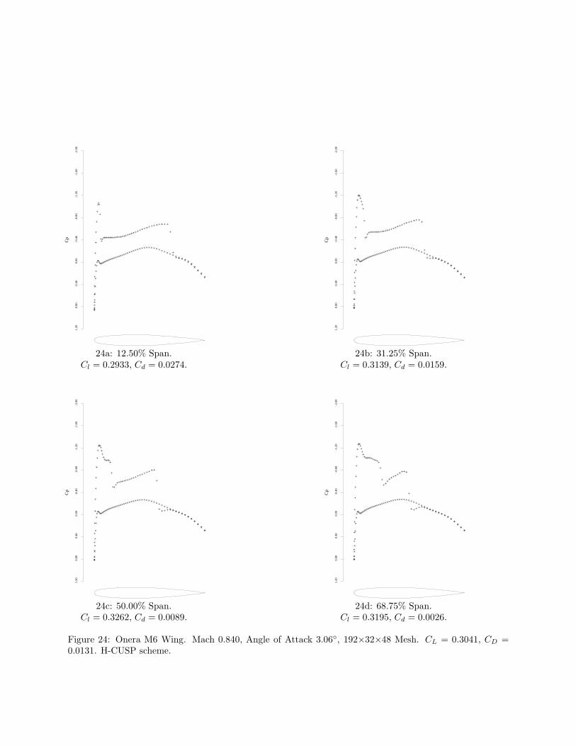
1.

20

0.80

0.

40

0.00

-0.

40 -

0.80

-1.

20 -

1.60

-2.

00

Cp

++

++

++++++++++++++++++++++++++++++++++++++++++++++++

+++++

+

+

+

+++++

+

+

+

+

+

+

+

+

+

+

+

+++

+

+++++++++++++++++++++++++++++++++++++ +

+

++ + + + +

++

++

+

24a: 12.50% Span.Cl = 0.2933, Cd = 0.0274.

1.

20

0.80

0.

40

0.00

-0.

40 -

0.80

-1.

20 -

1.60

-2.

00

Cp

++

++

+++++++++++++++++++++++++++++++++++++++++++++++++++

+

+

+

+

+

+++++

+

+

+

+

+

+

+

+

+

+

+

++++

++++

+

+++++

++++++++++++++++++++++++++

+

+ + + + + + + + ++

++

+

24b: 31.25% Span.Cl = 0.3139, Cd = 0.0159.

1.

20

0.80

0.

40

0.00

-0.

40 -

0.80

-1.

20 -

1.60

-2.

00

Cp

++

++

++++++++++++++++++++++++++++++++++++++++++++++++++++

+

+

+

+

+++++

+

+

+

+

+

+

+

+

+

+

+

+++++

+++++++++

+

++++++++++++++++++++++

+

+++ + + + + + + + + ++

++

+

24c: 50.00% Span.Cl = 0.3262, Cd = 0.0089.

1.

20

0.80

0.

40

0.00

-0.

40 -

0.80

-1.

20 -

1.60

-2.

00

Cp

++

++

++++++++++++++++++++++++++++++++++++++++++++++++++++

+

+

+

+

+++++

+

+

+

+

+

+

+

+

+

+

+

+++++

+++++++++++++++

+

+++

++++++++++

+

++++++ + + + + + + + + ++

++

+

24d: 68.75% Span.Cl = 0.3195, Cd = 0.0026.

Figure 24: Onera M6 Wing. Mach 0.840, Angle of Attack 3.06, 192×32×48 Mesh. CL = 0.3041, CD =0.0131. H-CUSP scheme.

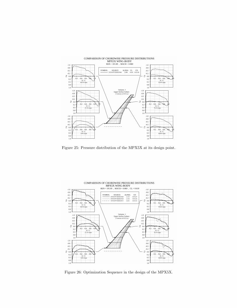
SYMBOL

SOURCE SYN107P DESIGN40

ALPHA 2.094

CL 0.610

CD 0.01126

COMPARISON OF CHORDWISE PRESSURE DISTRIBUTIONSMPX5X WING-BODY

REN = 101.00 , MACH = 0.860

Solution 1 Upper-Surface Isobars

( Contours at 0.05 Cp )

0.2 0.4 0.6 0.8 1.0

-1.0

-0.8

-0.5

-0.2

0.0

0.2

0.5

0.8

1.0

Cp

X / C 9.6% Span

0.2 0.4 0.6 0.8 1.0

-1.0

-0.8

-0.5

-0.2

0.0

0.2

0.5

0.8

1.0

Cp

X / C 27.2% Span

0.2 0.4 0.6 0.8 1.0

-1.0

-0.8

-0.5

-0.2

0.0

0.2

0.5

0.8

1.0

Cp

X / C 44.3% Span

0.2 0.4 0.6 0.8 1.0

-1.0

-0.8

-0.5

-0.2

0.0

0.2

0.5

0.8

1.0

Cp

X / C 60.8% Span

0.2 0.4 0.6 0.8 1.0

-1.0

-0.8

-0.5

-0.2

0.0

0.2

0.5

0.8

1.0

Cp

X / C 79.1% Span

0.2 0.4 0.6 0.8 1.0

-1.0

-0.8

-0.5

-0.2

0.0

0.2

0.5

0.8

1.0

Cp

X / C 95.6% Span

Figure 25: Pressure distribution of the MPX5X at its design point.

SYMBOL

SOURCE SYN107P DESIGN20

SYN107P DESIGN10

SYN107P DESIGN 0

ALPHA 2.113

2.153

2.251

CD 0.01127

0.01125

0.01131

COMPARISON OF CHORDWISE PRESSURE DISTRIBUTIONS MPX5X WING-BODY

REN = 101.00 , MACH = 0.860 , CL = 0.610

Solution 1 Upper-Surface Isobars

( Contours at 0.05 Cp )

0.2 0.4 0.6 0.8 1.0

-1.0

-0.8

-0.5

-0.2

0.0

0.2

0.5

0.8

1.0

Cp

X / C 9.6% Span

0.2 0.4 0.6 0.8 1.0

-1.0

-0.8

-0.5

-0.2

0.0

0.2

0.5

0.8

1.0

Cp

X / C 27.2% Span

0.2 0.4 0.6 0.8 1.0

-1.0

-0.8

-0.5

-0.2

0.0

0.2

0.5

0.8

1.0

Cp

X / C 44.3% Span

0.2 0.4 0.6 0.8 1.0

-1.0

-0.8

-0.5

-0.2

0.0

0.2

0.5

0.8

1.0

Cp

X / C 60.8% Span

0.2 0.4 0.6 0.8 1.0

-1.0

-0.8

-0.5

-0.2

0.0

0.2

0.5

0.8

1.0

Cp

X / C 79.1% Span

0.2 0.4 0.6 0.8 1.0

-1.0

-0.8

-0.5

-0.2

0.0

0.2

0.5

0.8

1.0

Cp

X / C 95.6% Span

Figure 26: Optimization Sequence in the design of the MPX5X.

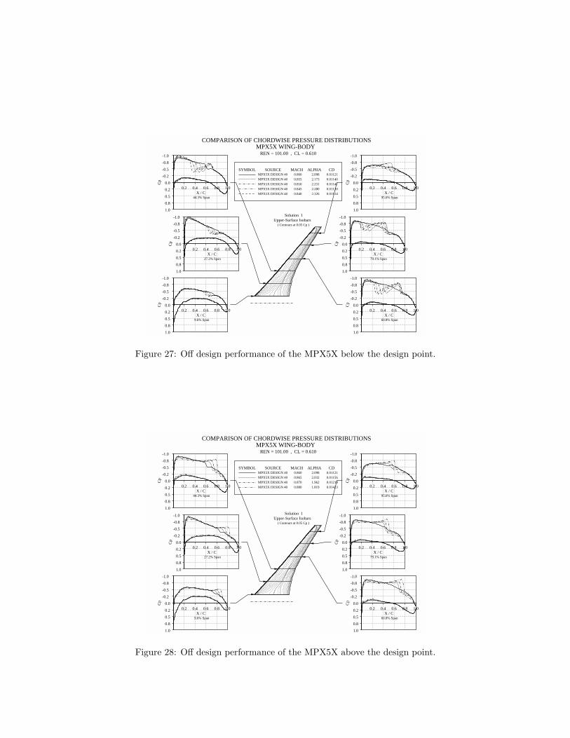
SYMBOL

SOURCE MPX5X DESIGN 40

MPX5X DESIGN 40

MPX5X DESIGN 40

MPX5X DESIGN 40

MPX5X DESIGN 40

MACH 0.860

0.855

0.850

0.845

0.840

ALPHA 2.098

2.173

2.231

2.280

2.326

CD 0.01121

0.01140

0.01141

0.01130

0.01114

COMPARISON OF CHORDWISE PRESSURE DISTRIBUTIONS MPX5X WING-BODY

REN = 101.00 , CL = 0.610

Solution 1 Upper-Surface Isobars

( Contours at 0.05 Cp )

0.2 0.4 0.6 0.8 1.0

-1.0

-0.8

-0.5

-0.2

0.0

0.2

0.5

0.8

1.0

Cp

X / C 9.6% Span

0.2 0.4 0.6 0.8 1.0

-1.0

-0.8

-0.5

-0.2

0.0

0.2

0.5

0.8

1.0

Cp

X / C 27.2% Span

0.2 0.4 0.6 0.8 1.0

-1.0

-0.8

-0.5

-0.2

0.0

0.2

0.5

0.8

1.0

Cp

X / C 44.3% Span

0.2 0.4 0.6 0.8 1.0

-1.0

-0.8

-0.5

-0.2

0.0

0.2

0.5

0.8

1.0

Cp

X / C 60.8% Span

0.2 0.4 0.6 0.8 1.0

-1.0

-0.8

-0.5

-0.2

0.0

0.2

0.5

0.8

1.0

Cp

X / C 79.1% Span

0.2 0.4 0.6 0.8 1.0

-1.0

-0.8

-0.5

-0.2

0.0

0.2

0.5

0.8

1.0

Cp

X / C 95.6% Span

Figure 27: Off design performance of the MPX5X below the design point.

SYMBOL

SOURCE MPX5X DESIGN 40

MPX5X DESIGN 40

MPX5X DESIGN 40

MPX5X DESIGN 40

MACH 0.860

0.865

0.870

0.880

ALPHA 2.098

2.032

1.962

1.819

CD 0.01121

0.01156

0.01219

0.01423

COMPARISON OF CHORDWISE PRESSURE DISTRIBUTIONS MPX5X WING-BODY

REN = 101.00 , CL = 0.610

Solution 1 Upper-Surface Isobars

( Contours at 0.05 Cp )

0.2 0.4 0.6 0.8 1.0

-1.0

-0.8

-0.5

-0.2

0.0

0.2

0.5

0.8

1.0

Cp

X / C 9.6% Span

0.2 0.4 0.6 0.8 1.0

-1.0

-0.8

-0.5

-0.2

0.0

0.2

0.5

0.8

1.0

Cp

X / C 27.2% Span

0.2 0.4 0.6 0.8 1.0

-1.0

-0.8

-0.5

-0.2

0.0

0.2

0.5

0.8

1.0

Cp

X / C 44.3% Span

0.2 0.4 0.6 0.8 1.0

-1.0

-0.8

-0.5

-0.2

0.0

0.2

0.5

0.8

1.0

Cp

X / C 60.8% Span

0.2 0.4 0.6 0.8 1.0

-1.0

-0.8

-0.5

-0.2

0.0

0.2

0.5

0.8

1.0

Cp

X / C 79.1% Span

0.2 0.4 0.6 0.8 1.0

-1.0

-0.8

-0.5

-0.2

0.0

0.2

0.5

0.8

1.0

Cp

X / C 95.6% Span

Figure 28: Off design performance of the MPX5X above the design point.

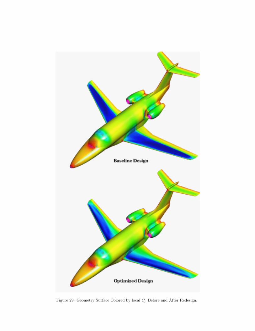
Figure 29: Geometry Surface Colored by local Cp Before and After Redesign.

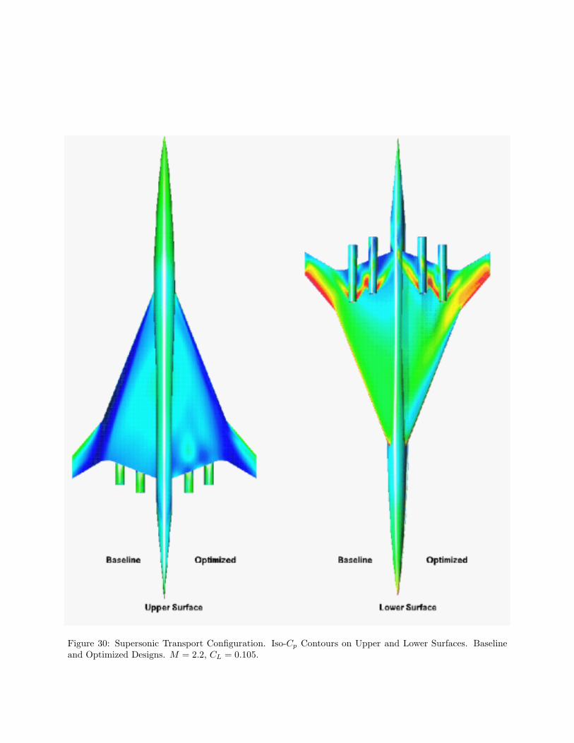
Figure 30: Supersonic Transport Configuration. Iso-Cp Contours on Upper and Lower Surfaces. Baselineand Optimized Designs. M = 2.2, CL = 0.105.

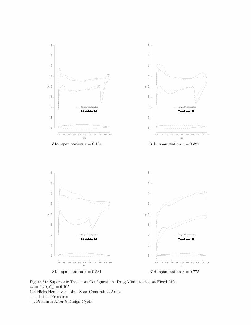
0.00 0.10 0.20 0.30 0.40 0.50 0.60 0.70 0.80 0.90 1.00

X/C

0.

32

0.24

0.

16

0.08

0.

00 -

0.08

-0.

16 -

0.24

-0.

32

Cp

Y stretch factor: 2.0 Y stretch factor: 2.0 Y stretch factor: 2.0 Y stretch factor: 2.0 Y stretch factor: 2.0 Y stretch factor: 2.0 Y stretch factor: 2.0 Y stretch factor: 2.0 Y stretch factor: 2.0 Y stretch factor: 2.0 Y stretch factor: 2.0

Original Configuration

Y stretch factor: 2.0 Y stretch factor: 2.0 Y stretch factor: 2.0 Y stretch factor: 2.0 Y stretch factor: 2.0 Y stretch factor: 2.0 Y stretch factor: 2.0

31a: span station z = 0.194

0.00 0.10 0.20 0.30 0.40 0.50 0.60 0.70 0.80 0.90 1.00

X/C

0.

32

0.24

0.

16

0.08

0.

00 -

0.08

-0.

16 -

0.24

-0.

32

Cp

Y stretch factor: 2.0 Y stretch factor: 2.0 Y stretch factor: 2.0 Y stretch factor: 2.0 Y stretch factor: 2.0 Y stretch factor: 2.0 Y stretch factor: 2.0 Y stretch factor: 2.0 Y stretch factor: 2.0 Y stretch factor: 2.0 Y stretch factor: 2.0 Y stretch factor: 2.0

Original Configuration

Y stretch factor: 2.0 Y stretch factor: 2.0 Y stretch factor: 2.0 Y stretch factor: 2.0 Y stretch factor: 2.0 Y stretch factor: 2.0

31b: span station z = 0.387

0.00 0.10 0.20 0.30 0.40 0.50 0.60 0.70 0.80 0.90 1.00

X/C

0.

32

0.24

0.

16

0.08

0.

00 -

0.08

-0.

16 -

0.24

-0.

32

Cp

Y stretch factor: 2.0 Y stretch factor: 2.0 Y stretch factor: 2.0 Y stretch factor: 2.0 Y stretch factor: 2.0 Y stretch factor: 2.0 Y stretch factor: 2.0 Y stretch factor: 2.0 Y stretch factor: 2.0 Y stretch factor: 2.0 Y stretch factor: 2.0 Y stretch factor: 2.0 Y stretch factor: 2.0

Original Configuration

Y stretch factor: 2.0 Y stretch factor: 2.0 Y stretch factor: 2.0 Y stretch factor: 2.0 Y stretch factor: 2.0

31c: span station z = 0.581

0.00 0.10 0.20 0.30 0.40 0.50 0.60 0.70 0.80 0.90 1.00

X/C

0.

32

0.24

0.

16

0.08

0.

00 -

0.08

-0.

16 -

0.24

-0.

32

Cp

Y stretch factor: 2.0 Y stretch factor: 2.0 Y stretch factor: 2.0 Y stretch factor: 2.0 Y stretch factor: 2.0 Y stretch factor: 2.0 Y stretch factor: 2.0 Y stretch factor: 2.0 Y stretch factor: 2.0 Y stretch factor: 2.0 Y stretch factor: 2.0 Y stretch factor: 2.0 Y stretch factor: 2.0

Original Configuration

Y stretch factor: 2.0 Y stretch factor: 2.0 Y stretch factor: 2.0 Y stretch factor: 2.0 Y stretch factor: 2.0

31d: span station z = 0.775

Figure 31: Supersonic Transport Configuration. Drag Minimization at Fixed Lift.M = 2.20, CL = 0.105144 Hicks-Henne variables. Spar Constraints Active.- - -, Initial Pressures—, Pressures After 5 Design Cycles.