A NOVEL MATRIX NEARNESS APPROACH FOR

FAST VOLTAGE COLLAPSE PROXIMITY ANALYSIS

K.C. HUI M.J. SHORT Department of Electrical and Electronic Engineering

Imperial College, London SW7 2BT, UK

ABSTRACT

This paper provides an analysis of power system voltage stability· in a Matrix Analysis Framework. In this framework, voltage collapse is presented as a Matrix Nearness problem using Matrix Theory to find a solution. A new Voltage Collapse Margin (VCM) called Minimum Relative Voltage Collapse Distance (MRVCD) has been developed to measure the relative distance from the present operating point to the nearest voltage collapse boundary. The margin is taken as a Voltage Collapse Indicator (VCI) for voltage collapse monitoring. The indicator properly conveys the deterioration of the voltage condition in power systems as the loading increases. Its simple and fast computational capability makes the indicator suitable for on-line voltage collapse assessment. The effectiveness of this voltage collapse evaluation method has been demonstrated on the IEEE 57 busbar system.

Keywords : Voltage Stability Monitoring, Matrix Analysis, Matrix Nearness Method, Matrix Theory, Standard Condition Number, Minimum Relative Voltage Collapse Distance

1. INTRODUCTION

The risk of voltage collapse in power systems is nowadays one of the major concerns in power system planning and operation (1 ],[2]. Toanalyze voltage instability, some researchers investigate the causes while others examine the nature of the phenomenon. In their analysis, researchers have noted the singularity of the Jacobian matrix of the power system equations at voltage collapse (2-7), (24-26]. Voltage collapse indicators (VCI) have been developed by detecting the singularity of the Jacobian. Voltage collapse margins (VCM) are measured as the distance from the Jacobian matrix of the power system to a singular matrix. Indices such as minimum eigenvalue llA I mrnl [4], minimum singular value (am1n) [6], Thevenin impedance ratio (Z1/Z1) [3], etc. have been used.

Voltage collapse evaluation methods based on singularity of the Jacobian matrix are important. However, like many other voltage collapse assessment methods, the evaluation methods developed so far suffer from:

1) inaccuracies due to the linearisation process in evaluation . of the VCls (19),(20];

2) inefficiency due to heavy computation, as in matrix decomposition [6] and non-linear optimization [7];

3) not being system-wide in assessment, but busbar specific [3],[19],[20], because the VCMs are formulated as the collapse margins at some specific vulnerable busbars, and not for the whole power system;

4) restrictions in practical use due to assumptions such as load conformity in development of the VCls [7];

5) invalidation due to problems such as inadequate power system modelling for the voltage analysis, unreliable behaviour of the power system algorithms in the vicinity of voltage collapse, etc., as discussed in [3].

_-I.II these problems (especially the demanding computational requirement of the methods) make these voltage collapse evaluation methods unsuitable for on-line monitoring and control.

The main objective of this paper is the development of new voltage collapse margin and voltage collapse indicators so that the evaluation method does not have the above mentioned problems and so will be effective and efficient for on-line voltage collapse monitoring. In this paper, voltage collapse problems are analyzed from the view point of singularity of the power system Jacobian. Singularity properties of the Jacobian and voltage collapse are studied in the Matrix Analysis Framework. A new voltage collapse margin (VCM) is formulated to measure the minimum distance between the present power system operating point and the voltage collapse boundary.

To find the explicit expression for the VCM, voltage collapse is presented as a Matrix Nearness Problem (8) in the analytical framework. Since voltage collapse is characterised by singularity of the Jacobian, the voltage collapse boundary becomes a class of Jacobian matrices which have the properties of singularity. Derivation of the minimum distance from the power system operating point to the voltage collapse boundary becomes a minimization process in which the member of the class of singular matrices ' nearest' to the Jacobian matrix of the present operating system is sought and the distance between the two matrices is evaluated. The 'nearest' is measured by the relative distance function which satisfies the general properties of the concept of ' length ' .

Matrix Theory [9],[1 OJ is employed to solve the minimization task. Since there is no requirement to identify any specific busbars in the minimization process, the VCM developed becomes a system­wide index which gives an overall voltage collapse margin for the whole power system. There is no linearisation nor does there need to be uniformity in loading increments in the development of the VCM, and so the VCM is effective for practical use. The VCI has a very simple computational form, making this indicator suitable for on-line voltage collapse monitoring.

In Section 2, the singularity property of a power system at voltage collapse is reviewed. Mathematical details of the singularity of the Jacobian matrix at voltage collapse are summarised. Section 3 formulates the new VCM and VCI for monitoring voltage collapse. To obtain the explicit expression for the VCM and VCI, voltage collapse problems are presented as Matrix Nearness problems in Section 4. Matrix Theory is employed to solve the problem and find the indices .

In addition to analyzing voltage collapse in the new analytical framework and proposing a new VCM and VCI for voltage collapse monitoring, the paper investigates various properties of the voltage collapse margin in Section 5. Various forms of the VCI are discussed. The relationship between the index and other voltage collapse indicators such as the Minimum Singular Value and the Minimum Eigenvalue is studied . Upper and lower bounds for the VCI are established. Fast methods are proposed in Section 6 to estimate the voltage collapse indicator and make it more computationally efficient for on-line voltage collapse monitoring. The effectiveness of this voltage collapse evaluation method is demonstrated on the IEEE 57 busbar system in Section 7.

2. SINGULARITY OF THE JACOBIAN MATRIX

Voltage collapse in a power system can be characterised by the singularity of the Jacobian of the system equations [2-7]. The

345

Jacobian concerned here could be the system Jacobian [3] , [4]

or (2.1)

if voltage collapse is analyzed in the dynamic domain, in which the power system behaviour is governed by a set of non-linear algebraic-differential equations

Q = §(2£,ld) ~ = E!&ldl

(2 .2a) (2.2b)

where the stator algebraic equations in §(2£,ld) = Q are implicitly embedded in the differential equations E(&ldl and functions §(2£,ld) =Qare network equations only.

If voltage behaviour of a power system is modelled by a set of non-linear power flow equations §(2£,ld) = Q and static voltage collapse, instead of dynamic voltage collapse, is analyzed, the Jacobian will be the Power-Flow Jacobian §.. [5-7] as deduced from the equations

d2£ dld (2 .3)

d( d(

which provides the basis of a characterisation of static voltage collapse and steady-state stability limits in the power system [6]. (is a scalar by which 2£ and .Jd are parameterised.

In general, which Jacobian is used for analyzing voltage collapse is immaterial because the two Jacobians are inter-related in such a way that if the non-linear differential equations k = E(&ldl are posed as~ = E(&ldl = !1.(Q.(~Jd)), where.hare the functions E in term of § and h(Q) = Q, then the solutions of the static equations §(2£,ld) = Q are equilibria of the dynamic equations k = E(&Jd). Bifurcation of solutions of §(2£,Jd) = Q implies bifurcation of the equilibria of~ = E(&Jd). Thus studying bifurcations of §(~,Jd) =Qin turn means studying bifurcations of the whole dynamic model (2 .2) whose steady-state behaviour is §(~,Jd) = Q. Characterising voltage collapse by singularity of the Power-Flow Jacobian §.. is the same as characterising voltage collapse by singularity of the System Jacobian (2. 1 ). If the general form, and not the particular details, of the dynamic model~ = E(&Jd) is given, voltage collapse can always be studied with the static model §(~ld) = Q and the Power-Flow Jacobian § x.

3 . THE MINIMUM RELATIVE VOLTAGE COLLAPSE DISTANCE

Characterising voltage collapse in power systems by singularity of the Jacobian matrix, the voltage collapse boundary becomes a class of singular matrices, or a group of power system operating points, whose Jacobian matrices have singularity properties. The distance between a power system operating point and the voltage collapse boundary (i.e. Voltage Collapse Margin VCM) becomes the distance between the Jacobian matrix of the power system and the class of singular matrices. The minimum distance from a power system operating point to the voltage collapse boundary becomes the distance from the Jacobian matrix to the member of the singular matrices which is "nearest" to the Jacobian matrix. If "nearest" is measured by a· relative distance function, the distance becomes the minimum relative distance between the power system operating point and the voltage collapse boundary. This distance is called the Minimum Relative Voltage Collapse Distance (MRVCD) in this paper.

Using this Minimum Relative Voltage Collapse Distance (MRVCD) as voltage collapse indicator (VCI), voltage collapse in power systems can be evaluated as

\ VCI = MRVCD > 0 =<>{system is voltage stable} \ (3.1) ' VCI = MRVCD -+ 0 =<>{system is voltage unstable}

4. VOLTAGE COLLAPSE ANALYSIS IN MATRIX ANALYSIS FRAMEWORK

To find the explicit expression for the Minimum Relative Voltage Collapse Distance (MRVCD), the voltage collapse problem is presented as the following Matrix Nearness Problem .

4.1 Matrix Nearness Problem

The Matrix Nearness Problem in Matrix Analysis [8) consist of finding, for an arbitrary matrix A, a ' nearest" member of some given class of matrices. The ' nearest" is measured by a distance function which satisfies the general properties of the concept of "length" discussed in [11 ].

find BE M"' such that d(A,B) is minimized

where d(A,B) is a distance function showing the distance between matrix A and matrix B; McP is a class of matrices which have matrix property rP. Mathematically, the problem can be presented as a minimization problem in which

m1n1m1ze d(A,B) subject to : B E M"'

In general, there is no restriction on the choice of the distance function d( •) for matrix nearness problems . However, for tractability of the nearness problem, the matrix norm II • II is generally used. Using the Holder norm (the generalised p-mat rix norm [11 ]) as the distance function and considering E = B - A, the matrix nearness problem can be re-formulated as: For a matrix A.

or simply,

minimize : d(A) = II E II P

subject to : A + E E M"'

minimize: d(A) = {ii Eli•: A + E E M"'} (4.1)

It can be seen that magnitude of the distance function d(A) depends greatly upon the choice of the matrix norm II • II •. Sometimes it is more convenient to use the relative distance to reduce this dependency. For a relative distance function d(A) = II E II P I II A II P , the Matrix Nearness problem becomes

II Ell. minimize : d(A) = {- : A + E E M"'} (4 .2)

llAllP Equation (4.2) in fact suggests that the matrix nearness problem is the problem of finding the "smallest ' matrix E for matrix A so that some matrix property M"' is induced to matrix A. "Smallest " in the problem is measured through the "size" of the matrix E relative to the 'size" of the matrix A and the "sizes' of the matrices are measured by the matrix norm II • II p·

4.2 Matrix Nearness Approach to Voltage Collapse Problem

Characterising voltage collapse by singularity of the Jacobian matrix §.. (or [J) for simplicity) and presenting voltage collapse problems as matrix nearness problems in matrix analysis, a relative distance function is constructed

II t.J II p

d(J) = {-- : J + t.J E R"xn is singular, J and l!.J E R"' "}

II J II p

or more mathematically,

II t.J II. d(J) = {-- : (J + t.J).li = Q, ~ ~ Q E R", J and t.J E R"x"}

346

llJ II p (4.3)

To minimize the relative distance d(J) over all nonzero .li and under the constraints (J + t.J).li = Q, the following Matrix Theory

[9]. [1 OJ is applied. Considering

(J + AJ) = J(I + J·1£lJ) (4.4)

Since [JJ is non-singular, equation (4.4) is satisfied if and only if (I + J·1 llJ) is singular, i.e.

where .1i '# Q

~ llJ"1AJ.1illp = hiiP

~ P 1 II p llllJ II p blip ~ lldp

ll AJllP

II J II p

(4.5)

Therefore, minimization of d(J) in (4.3) is equivalent to finding a AJmin which achieves the equality in equation (4.5). that is llAJminllP/ llJllP = 1 I llJllPIJJ·

1JIP = min<llAJJIP I llJIJP}.

Let us consider a vector z. for which

By putting AJ = -z. !E.T

then z. = -AJJ·1z.

(For evaluation of the dual vector fE., please refer to the Appendix). Since J·1z. ;e Q, (J + AJ) is singular. AJ = -z. !E.T is therefore a matrix with which (J + AJ) is singular. Also,

llAJll. llAJ.lillP --=-- max

II J II p llJ 11. .li'#Q blip

11-l_ fE.T.lill P max

llJ II p .li'#Q blip

1 lfE.T.lil = - llz.llP max

llJllP _li'#Q lldp

1

= - lldp ll!E.TllP II J II p

1 =- hllp

llJllP P 1z.llP

1 1

= - llz.llp llJllP P 1

llpllz.llp

llJllP P 1 II.

IJAJ lip = min{--}

II J II p

Therefore, the minimum value of the relative distance function d(J) is

Kp(J)

This minimum value of the relative distance function is the Minimum Relative Voltage Collapse Distance defined in Section 3. The scalar II J II P llJ"1 II P in the equation is called the Standard Condition Number in p-matrix norm (12) and is denoted by KP(J). The condition number is also called the condition number of the matrix [JJ with respect to inversion because the number is derived with respect to the singularity or non-invertibility of the matrix [J). It can be seen that by considering different matrix properties M"' in equation (4.1) in the matrix nearness problem, different condition numbers with respect to different problems will be formulated; for example the condition number with respect to eigenvalue problems (11 ), etc.

This minimum relative distance is used as the voltage collapse indicator (VCI).

(4.6)

The voltage collapse indicator is an inverse of the condition number. It can easily be determined by evaluating norms of the two matrices, the Jacobian matrix and its inverse, which is readily available from some algorithms in power system analysis such as the load flow analysis used in dynamic simulation and in power flow studies. High computational efficiency of the VCI means that the voltage collapse evaluation method is fast enough for on-line voltage collapse monitoring. Simplicity of the VCI formulation suggests that the VCI can be incorporated into the reactive power dispatch algorithm (21 I for maintaining, as well as monitoring, the voltage security of power systems.

5. CHARACTERISTICS OF THE MRVCD

5.1 Bounds for the MRVCD

In Sections 3 and 4, voltage collapse is assessed by the MRVCD which is evaluated as the inverse of the Standard Condition Number, Kp(J)·1 • The MRVCD shows the minimum relative distance between a power system operating point and the collapse boundary. If the MRVCD is small, the Jacobian of the system equations is near to being singular, ,and the power system is near to voltage collapse. However, what is meant by a "small" value for the MRVCD in this context? To make this more precise, the lower and upper bounds for the distance measure have to be established.

5.1.1 Upper Bound - For a vector norm or a matrix norm [13),

""" Kp(J) = II J II p P 1 II p ~ 1

""" Kp(J)·1 = Ill J II p P 1 II p) •l ::;;

Therefore, unity is the upper bound of the MRVCD. Thus, in speaking of a 'small value of MRVCD" for detecting voltage collapse, we mean the indicator is "small' relative to unity.

5.1 .2 Lower Bound - Theoretically, the lower bound for the MRVCD is zero, where the Jacobian [J] is singular, and the voltages in the power system have completely collapsed. However, at voltage collapse, load flow analysis will never

347

converge. The Jacobian matrix [J) and its inverse cannot be determined for computation of the MRVCD. To define the MRVCD at the voltage collapse situation, a lower bound has to be established for the distance. If the MRVCD value is lower than the established lower bound, the power system is said to have collapsed.

The question of the lower bound depends on how close operators would allow power systems to operate from their collapse boundaries. Obviously, the nearer a power system is allowed to operate to its collapse boundary, the smaller will be the lower bound for the MRVCD in voltage collapse monitoring . However, in any case, the permissible MRVCD in voltage collapse monitoring should not be smaller thanµ, whereµ is the rounding unit of the floating-point representation of the computing machine and is called the "machine unit' in Numerical Computation (14). If the MRVCD is smaller than the machine unitµ, the computed solution vector dlS/d(for the power system equations (2.3) is likely to have no correct digits in each component, and the power system equations cannot be properly solved. The Jacobian matrix§.. or [J) cannot then be correctly determined, and so the MRVCD cannot be correctly evaluated. The situation is said to be absolutely ill­conditioned with respect to the precision of the computing machine (16), and the power system should be declared to be collapsed from a numerical stability point of view. Therefore, the minimum lower bound for the MRVCD isµ.

5.2 The MRVCD. Singular Value o. and Eigenvalue A

Definition of the MRVCD in (4.6) involves the condition number in a matrix norm. Different matrix norms will give rise to different MRVCD values and to different names for the condition number (11 ). For example, if the Euclidean norm II • II E (or called Frobenius norm II • II F) is used, then the condition number Ke is called the Euclidean Condition Number; for L2-norm, the condition number K 2

is called the Spectral Condition Number. The MRVCD in L2-matrix norm has a very interesting property. That is (11)

if [J) is symmetric

where 1<., o, and A are the condition number, singular value, and eigenvalue of the Jacobian matrix [J) respectively. If II J 112 = 1 is taken, which can always be achieved by multiplying the power system equations (2.3) by a suitable constant, then

MRVCD = II J·1 II 2 = Omin

= IAlmln if [J] is symmetric

and so assessment of voltage collapse by the MRVCD with normalised Jacobian matrix in L2-matrix norm is the same as the Minimum Singular Value method (6) and the Minimum Eigenvalue method. Voltage collapse is detected by MRVCD = K2(J)·1 = omin = 0 . In fact, it can be seen that the proposed voltage collapse assessment method by the MRVCD is a generalisation of the Minimum Singular Value method and the Minimum Eigenvalue method . The Minimum Singular Value method, first introduced by Tiranuchit and Thomas (6), was further developed and made computationally efficient by Lof, et. al. (22]. (23) . The successful applications of the method for power systems with thousands of nodes proved its practical value in voltage collapse monitoring.

6. COMPUTATION OF THE MRVCD

The Minimum Relative Voltage Collapse Distance is a good indicator for assessing voltage collapse in power systems . Unfortunately, this is not an inexpensive quantity to compute because the indicator requires the inversion of the Jacobian matrix [J). Computation of the inverse of a near-singular 111atrix is very inefficient, and the solution is inexact. To make the voltage collapse assessment methods accurate and fast enough for on-line

use, the following methods are suggested for computing and estimating the Minimum Relative Voltage Collapse Distance.

6.1 with [J) and [J·1] obtained from Load Flow Analysis

In the N-R method of load flow analysis for a power system, §(y,20 = Q, basic repetitive iterations involve solving the linear state equations

(6 .1)

and then updating the state vector ~1•+ 1 1 = ~1 •1 + ~M • The solution procedure (6 .1) in the Newton's power-flow method actually suggests that the Jacobian matrix [J) and its inverse [J·1

]

are readily available for voltage stability assessment. Therefore, the MRVCD of the voltage collapse assessment method can easily be computed with the two matrices [JI and [J·11 available from load flow analysis.

6.2 Estimation of the MRVCD with random b1 vectors

For a large power system, the Jacobian matrix [J) in load flow analysis can have dimensions of thousands by thousands . Direct inversion of such a large matrix of millions of elements for load f low analysis is not feasible. To make load flow analysis practically viable for large power systems, many methods have been developed to solve the iterative procedure (6. 1) for ~M without directly inverting the Jacobian matrix [J); and the most popular method probably is the Gaussian Elimination (G-E) method.

In load flow analysis, if the linear state equations (6.1) are solved by the G-E method, then [J·1] is not available from load flow analysis for computing the MRVCD. To obtain the MRVCD for voltage collapse monitoring in that case, the MRVCD has to be

estimated without finding [J·1] as follows (14):

Now, if J E R"xn is invertible, then for an arbitrary vectors ~ and Q

J~ = Q (6 .2)

~ hllp :s P 1ll p 11211p

11.Qllp ~ :s llJllP., --

llJllP P 1llp ll 2S.llp

llQ llP ~ lnfimum llJllP., --

llJ llP P 1llp V.Q.~Q ll2S. ll.

(6.3)

Selecting k vectors B = {.Q1, .Q2, ... , 11.k} at random and solving equation J2S,1 = l1_1 fort_, where 1 :s i :s k. Equation (6.3) becomes

MRVCD 1 II 12; II p

= min llJll; 1 --

llJllP P 1llp 1 :Si:Sk ll2S.

1ll.

This estimate requires little additional computation effort because the multipliers for solving J2S, = Q have already been computed by the G-E method in the iterative procedure (6.1) of load flow analysis and has been stored in the memory. Determination of each ~1 , therefore, requires only an additional n2 mathematical (multiplication/divisions) operations, and so estimation of the MRVCD requires only about kn2 mathematical operations in addition to computation of II J II p· For n large, it is a small additional computation compared to the load flow problem, and for n small, all of the computations are inexpensive.

6.3 Estimation of the MRVCD with special b1 vectors

In Section 6.2, it has been suggested that the MRVCD can be estimated by a set of random choice of .Q1 vectors. However, to have an accurate estimate, one needs a large number of .Q1 vectors

348

to push the II hi II pi II ~i II P division to its infimum and so the estimation method is not efficient.

To improve the accuracy and efficiency of the estimation algorithm, the authors suggest a modification of the method in the following way, depending on how accurate and how efficient the estimation method is required to be. The technique is based on modifying the choice of the hi vector set.

1)

2)

Choose the hi vector set so that all h1 in the vector set are non-repeated random vectors, Choose b1 vector set from the set of Standard Basis which spans Rn: i.e. B = {g1 I 1 s i s k}, where g1 is the i'h Standard Basis of lR" . Of course if k = n, where n is the dimensionality of the Jacobian [J]. then the exact value of the MRVCD will be found because inverting the matrix [J) is the same as solving the set of simultaneous equations [J)[X] = [U), where [U] = [g1 ,g2

, ••• &"]. This estimation method guarantees that the exact value of the MRVCD can

be found and the number of h1 vectors required in the estimation is limited to be less than n.

3) Compute the MRVCD with LINPACK estimate (15).(17) of II J·1 11 p· The method chooses a special vector for vector h so that the vector .b. is a vector with ± 1 entries. This choice of .Q is somewhat technical, and readers interested in this are advised to refer to reference [15] . Further, once ~is found by solving the equations J~ = h with Q being the special vector, a vector y is computed from JTy = ~. II J· 1 II P

is estimated by II Y 11 P I II~ II P and the MRVCD is computed as

MRVCD

Ttie computational effort of this approach is about the same as that described in Section 6.2 with k=3.

6.4 Estimation of the upper-bound value for the MRVCD

Instead of estimating the exact value of the MRVCD for voltage collapse monitoring, another method is to estimate an upper-bound value for the indicator. At voltage collapse, row operations applied to equation (2.3) for triangularising the Jacobian matrix [J) of the equation will not affect the data vector d!!/d( of the equation because dy/d( is a null vector at voltage collapse situation. Equation (2.3) at voltage collapse still holds with [J] being triangularised and d!!/d( = Q. This equation in turn means that the triangularised Jacobian matrix at voltage collapse is singular. Voltage collapse characterised by singularity of the Jacobian matrix can thus also be characterised by singularity of the triangularised Jacobian matrix.

In load flow analysis with G-E method for solving the linear state equations (6.1 ), the Jacobian matrix of the power system is triangularised for back-substitution. With the triangular Jacobian matrix obtained from the load flow analysis and with voltage collapse characterised by singularity of the triangular Jacobian matrix, the MRVCD for voltage collapse monitoring can be estimated as [16)

MRVCD s

It is known that all diagonal entries of the triangular Jacobian matrix are nonzero, and that replacing any diagonal entry of the triangular Jacobian by zero makes the Jacobian matrix singular and non-invertible. The MRVCD estimated with the above equation in the situation becomes zero, and according to equation (3. 1 ), the voltage of the power system is concluded to be collapsed.

This method gives the fastest estimation for the MRVCD because, instead of finding the inverse of the Jacobian for the MRVCD, it is only necessary to find the minimum diagonal entries of the triangular Jacobian matrix. The estimated indicator gives system

operators an upper-bound value for assessing voltage collapse conditions in power systems. If the estimated MRVCD is already a small value, the voltages of a power system can be considered to have collapsed. No further computation is needed for an exact

value of the MRVCD because the exact value of the MRVCD must be less than the estimated one and the indicator with an exact value should give the same conclusion as its estimate does.

7. RESULTS

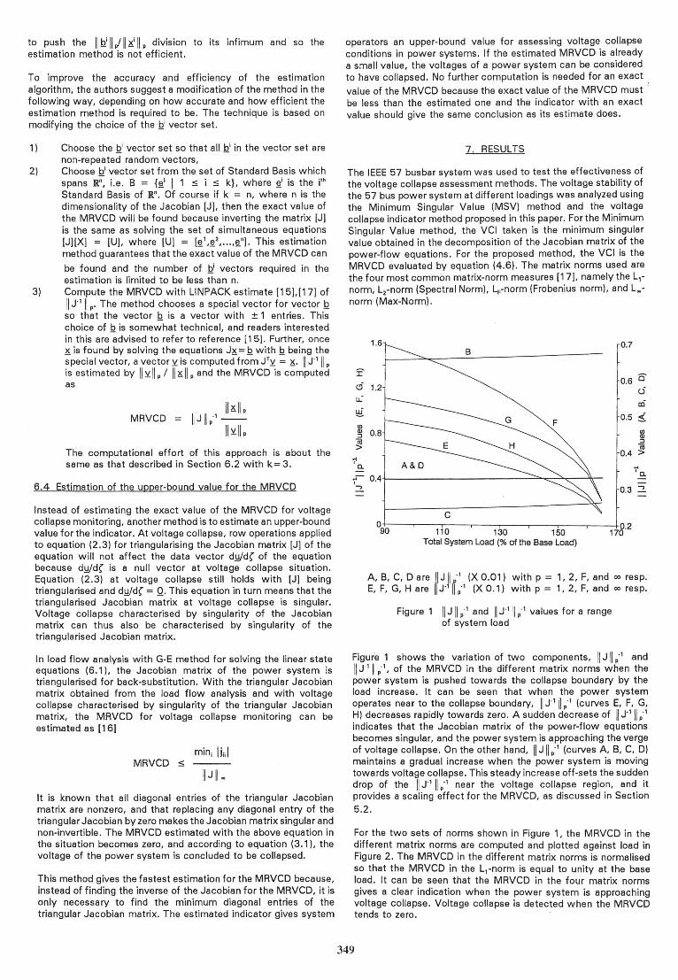
The IEEE 57 busbar system was used to test the effectiveness of the voltage collapse assessment methods. The voltage stability of the 57 bus power system at different loadings was analyzed using the Minimum Singular Value (MSV) method and the voltage collapse indicator method proposed in this paper. For the Minimum Singular Value method, the VCI taken is the minimum singular value obtained in the decomposition of the Jacobian matrix of the power-flow equations. For the proposed method, the VCI is the MRVCD evaluated by equation (4.6). The matrix norms used are the four most common matrix-norm measures [17). namely the L,­norm, L2-norm (Spectral Norm), LF-norm (Frobenius norm). and Lm­norm (Max-Norm).

I' cj

u: ~ Ul Q) :J iii > ,. a.

-:--,

1.6 0.7

0.6 El 1.2 c5

ai

0.5 ~ O.B 8l

:J iii

0.4 > ...

0.4 'a.

0.3 -,

0.2 170

0:1::-~.-~-,..-~-,.~~..--~.-~-.-~~~--+

90 110 130 150 Total System Load (% of the Base Load)

A, B. C, Dare \I J.jl r·1_1 (X 0.01) w.ith p = 1, 2, F, and oo rasp.

E, F, G, Hare I J I P (X 0.1) with p = 1, 2, F, and oo resp.

Figure 1 II J II P. , and II J·1 II P. , values for a range of system load

Figure 1 shows the variation of two components, II J II P. , and II J·1 II P. ,, of the MRVCD in the different matrix norms when the power system is pushed towards the collapse boundary by the load increase . It can be seen that when the power system operates near to the collapse boundary, II J·1 II P. , (curves E, F, G, H) decreases rapidly towards zero. A sudden decrease of II J·1 II P.,

indicates that the Jacobian matrix of the power-flow equations becomes singular, and the power system is approaching the verge of voltage collapse. On the other hand, II J II/ (curves A, B, C, D) maintains a gradual increase when the power system is moving towards voltage collapse. This steady increase off-sets the sudden drop of the II J·1 II P. , near the voltage collapse region, and it provides a scaling effect for the MRVCD, as discussed in Section 5.2.

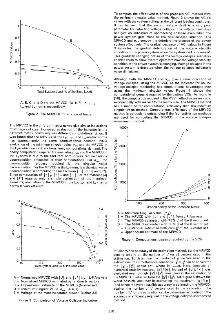
For the two sets of norms shown in Figure 1, the MRVCD in the different matrix norms are computed and plotted against load in Figure 2. The MRVCD in the different matrix norms is normalised so that the MRVCD in the L,-norm is equal to unity at the base load. It can be seen that the MRVCD in the four matrix norms gives a clear indication when the power system is approaching voltage collapse. Voltage collapse is detected when the MRVCD tends to zero.

349

0.8

Ul (!) :l (ij

0.6 > 0 t) > a: :E 0.4

0.2

B

c

To compare the effectiveness of the proposed VCI method with the minimum singular value method, Figure 3 shows the VCls's values with the system voltage at the different loading conditions. It can be seen that the system voltage itself is a very poor parameter for detecting voltage collapse. The voltage itself does not give an indication of approaching collapse even when the power system gets close to the near-collapse situation. The MRVCD and amln convey the deteriorating process of the power system effectively. The gradual decrease of VCI values in Figure 3 indicates the gradual deterioration of the voltage stability condition of the power system when the system load is increased. This gradually changing nature of the voltage collapse indicators enables them to show system operators how the voltage stability condition of the power system is changing. Voltage collapse in the power system is detected when the voltage collapse indicator's value diminishes.

Although both the MRVCD and am1n give a clear indication of voltage collapse, using the MRVCD as the indicator for on-line

0 90 110 130 150

Total System Load (% of the Base Load)

A, B, C, and D are the MRVCD (X 10·3 ) in L1, L2,

LF• and Lm-norms respectively

Figure 2 The MRVCDs for a range of loads

170 voltage collapse monitoring has computational advantages over using the minimum singular value. Figure 4 shows the computational demand required by the various VCls. As found in (18], the computation required in the MSV method increases cubic exponentially with respect to the matrix size. The MRVCD method has a much better computational · efficiency than the minimum singular value method. Computational efficiency of the MRVCD method is particularly outstanding if the fast estimation methods are used for computing the MRVCD in the voltage collapse assessment method.

The MRVCD in the different matrix norms give similar indications of voltage collapse. However, evaluation of the indicator in the different matrix norms requires different computational times. It was found that the MRVCD in the L1-, LF-, and Lm-matrix norms has approximately the same computational demand, while evaluation of the minimum singular value amln and the MRVCD in the L2-matrix norm suffers from heavy computational demand. The heavy computation required for evaluating omin and the MRVCD in the L2-norm is due to the fact that both indices require tedious decomposition processes in their computations. For amin• the decomposition process required is the singular value de.composition. For the MRVCD in the L2-norm, it is the eigenvalue decomposition in computing the matrix norm II • 11 2 of [J) and [J·1].

Since computation of II • 11 1• II • II F• and II • II m of the matrices [J] and [J·11 requires only a simple summation of the matrices' elements, evaluation of the MRVCD in the L,-, LF-· and Lm-matrix norms is very efficient.

1.1

1.4 0.9

(!) :> Oi >

0.7 0

l;; :;

u Cl > a: :::!<

0.5

c: (jj

E :> E

0.3

0.6 ·c: ~

B .Jll c

0.2 110 130 150 170

Total System Load (%of the Base Load)

A = Normalised MRVCD with II J II and II J·1 II from L-F Analysis B = Normalised MRVCD estimated by random _Qi vectors C = Upper-bound estim_ate of the MRVCD (Normalised) D = Minimum Singular Value omin (X 0.1) E = Voltage at the most vulnerable busbar (Busbar 33)

Figure .3 Comparison of Voltage Collapse Indicators

4000

~ Ul (3 3000 > (!)

£ '-

.E (!)

E 2000 t= Cii c:

A

0

~ a. 1000 E

B c D

0 (.)

Dimensionality of the Jacobian Matrix

A = Minimum Singular Value (am1nl B = The MRVCD with II J II and 11 J·1 II from L-F Analysis C = The MRVCD estimated with 75% _Qi of the B vector set D = The MRVCD estimated with 50% b1 of the B vector set E = The MRVCD estimated with 25% _iii of the B vector set F = Upper-bound estimate of the MRVCD

Figure 4 Computational demand required by the VCls

E

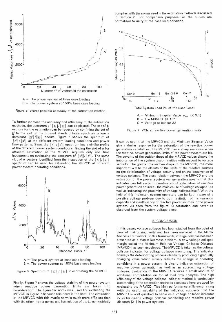
Efficiency and accuracy of the estimation methods for the MRVCD depend greatly on the number of .Q1 (or .!!_i) vectors used in the estimation. To determine the number of e1 vectors used in the estimations, the simultaneous equations Ji= !!1 can be solved for the II ~1 II I II !:!_1 II scalar set, where i = 1, ... ,n. Here, because of numerical stability reasons, II~ \I I II !:!.1 II instead of II !!1 II I II ~1 II was evaluated even though II !!1 II I II~ /I was used in the estimation of the MRVCD. Evaluated from the I ~1 II I II !!1 II set, Figure 5 shows the worst possible accuracy in estimating the maximum II ~1 II I I I ~ II (and hence the worst possible accuracy in estimating the MRVCD) against the number of .Q1 vectors used in the estimation. The number of .Q1 for the estimation can be determined according to the accuracy or efficiency required in the voltage collapse assessment method.

350

"'O Q)

1ii E -~ Q)

Q) :J (ii >

·-Q)

x

E :J

E ·x ro ~

'§ 0 3

®001

40001

i I

2000~ I I

J 0

;8 I

I J

(

! I

I (

/",~

I

2o 4o . 60 80 160 Number of e 1 vectors in the estimation

A = The power system at base case loading B = The power system at 150% base case loading

Figure 5 Worst possible accuracy of the estimation method

To further increase the accuracy and efficiency of the estimation methods, the spectrum of 11 K i II I II ~i II can be plotted . The set of li vectors for the estimation can be reduced by confining the set of Qi to the slot of the ordered standard basis spectrum where a dominant II Ki II I II ~i II occurs. Figure 6 shows the spectrum of II Ki II I II ~i II at the different system loading conditions and power flow patterns. Since the hi II I II ~1 11 spectrum has a similar profile at the different power system conditions, finding the slot of gi for efficient estimation of the MRVCD requires only one time investment on evaluating the spectrum of II Ki II I II ~i II· The same slot of g1 vectors identified from the inspection of the II Ki II I II ~i II spectrum can be used for estimating the MRVCD at different power system operating conditions.

l ! 6000~ 1\s I

j I

1 I

Ill I Q)

4000~ I :J (ii

\ > I I

Q) 1 x

2000

20 40 60 80 100 Standard Basis ei

A = The power system at base case loading B = The power system at 150% base case loading

Figure 6 Spectrum of II Ki I! I II ~i II in estimating the MRVCD

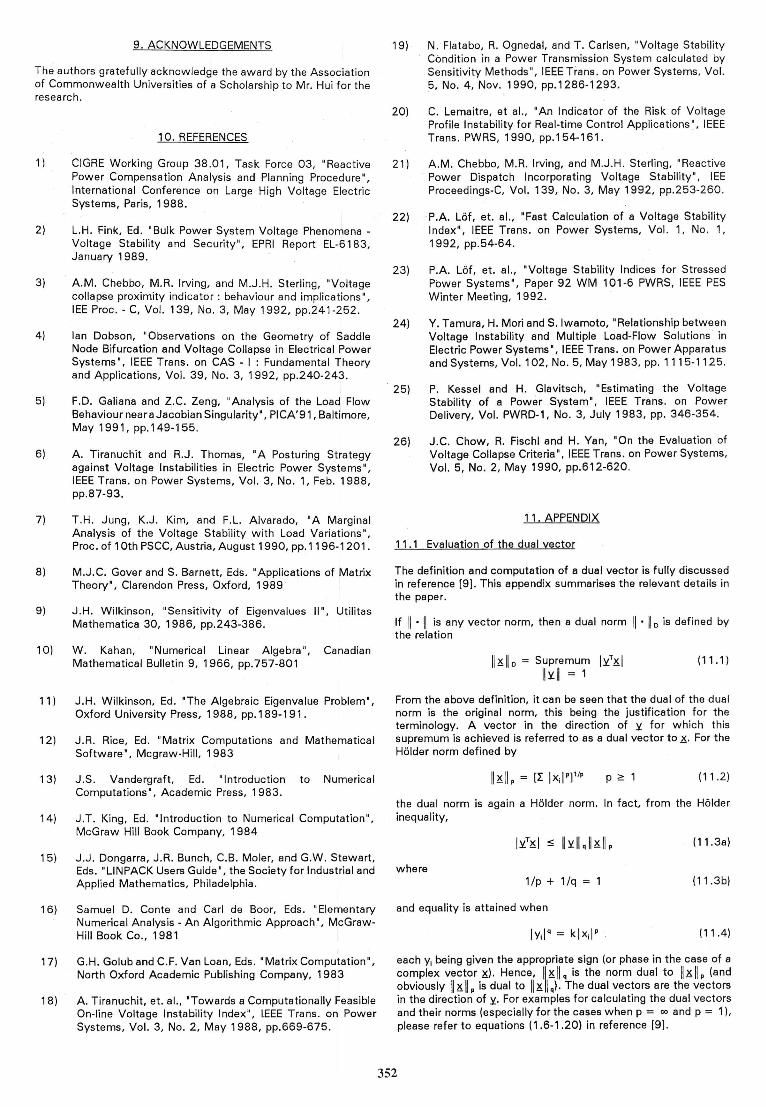
Finally, Figure 7 shows the voltage stability of the power system when reactive power generation limits are taken into consideration . The L, -matrix norm was used for evaluating the MRVCD in Figure 7 because this norm is the best. The evaluation of the MRVCD with this matrix norm is much more efficient than with the other matrix-norms and formulation of the L,-norm strictly

complies with the norms used in the estimation methods discussed in Section 6 . For comparison purposes, all the curves are normalised to unity at the base load condition .

1.6

QJ 1.2

::J (ii > iii :; Dl

0 Bi c en E ::J E ·c:

0 . 4 ~ ~

0 90

Gen 9 Gen 12 Gen 3 & 6 Gen 2

110 130 150 95 117 130 143

Total System Load {% of the Base Load)

A = Minimum Singular Value omin (X 0 .1) B = The MRVCD (X 1 0·4 )

C = Voltage at busbar 33

Figure 7 VCls at reactive power generation limits

! 3

L2 I i Cl

~ u >

I a: :::!'

0

It can be seen that the MRVCD and the Minimum Singular Value give a similar response for the saturation of the reactive power generation capabilities . The MRVCD has a sharp response when the reactive power generation limits of the power system are hit . The severity of the sudden drops of the MRVCD values shows the importance of the system discontinuities with respect to voltage security. The greater the sudden drops of the MRVCD, the more important will be the effects of the limits of the reactive sources on the deterioration of voltage security and on the occurrence of voltage collapse. The close relation between the MRVCD and the saturation of the power system var generation means that this indicator can tell system operators about exhaustion of reactive power generation sources - the main cause of voltage collapse - as well as indicating the proximity of voltage collapse itself. With the help of this indicator, system operators can be kept aware of a possible voltage problem due to both limitation of transmission capacity and insufficiency of reactive power sources in the power system. As seen from the figure, Q saturation can never be observed from the system voltage alone.

8. CONCLUSION

In this paper, voltage collapse has been studied from the point of view of matrix singularity and has been analyzed in the Matrix Analysis Framework. In this framework, voltage collapse has been presented as a Matrix Nearness problem. A new voltage collapse margin called the Minimum Relative Voltage Collapse Distance (MRVCD) has been developed. The MRVCD is taken as the voltage collapse indicator for voltage collapse monitoring. The indicator conveys the deteriorating process clearly by producing a gradually changing value which closely reflects the change in operating

conditions in a power system. It clearly indicates saturation of reactive power generation as well as an approaching voltage co llapse . Evaluation of the MRVCD requires a small amount of additional computation on top of load flow analysis. The high efficiency of the voltage collapse indicator method is particularly outstanding if the estimation methods disc·ussed here are used for evaluating the MRVCD. This high performance efficiency, along with the useful capability of the indicator, suggests that the MRVCD is well qualified to serve as a voltage collapse indicator (VCI) for on-line voltage collapse monitoring and reactive power dispatch [211 in power systems.

351

9. ACKNOWLEDGEMENTS

The authors gratefully acknowledge the award by the Association of Commonwealth Universities of a Scholarship to Mr. Hui for the research.

1)

2)

3)

4)

5)

6)

7)

8)

9)

1 0. REFERENCES

CIGRE Working Group 38.01, Task Force 03, "Reactive Power Compensation Analysis and Planning Procedure", International Conference on Large High Voltage Electric Systems, Paris, 1988.

L.H. Fink, Ed. "Bulk Power System Voltage Phenomena -Voltage Stability and Security", EPRI Report EL-6183, January 1989.

A.M . Chebbo, M.R. Irving, and M.J.H. Sterling, "Voltage collapse proximity indicator : behaviour and implications", IEE Proc. - C, Vol. 139, No. 3, May 1992, pp.241-252.

Ian Dobson, "Observations on the Geometry of Saddle Node Bifurcation and Voltage Collapse in Electrical Power Systems", IEEE Trans. on CAS - I : Fundamental Theory and Applications, Vol. 39, No. 3, 1992, pp.240-243.

F.D. Galiana and Z.C. Zeng, "Analysis of the Load Flow Behaviour neara Jacobian Singularity", PICA'91, Baltimore, May 1991, pp.149-155.

A. Tiranuchit and R.J. Thomas, 'A Posturing Strategy against Voltage Instabilities in Electric Power Systems", IEEE Trans. on Power Systems, Vol. 3, No. 1, Feb. 1988, pp.87-93.

T .H. Jung, K.J. Kim, and F.L. Alvarado, "A Marginal Analysis of the Voltage Stability with Load Variations', Proc. of 1 Oth PSCC, Austria, August 1990, pp.1196-1201.

M.J.C. Gover and S. Barnett, Eds. 'Applications of Matrix Theory", Clarendon Press, Oxford, 1989

J.H. Wilkinson, "Sensitivity of Eigenvalues 11', Utilitas Mathematica 30, 1986, pp.243-386.

10) W. Kahan, "Numerical Linear Algebra ", Canadian Mathematical Bulletin 9, 1966, pp. 757-801

11) J.H. Wilkinson, Ed. 'The Algebraic Eigenvalue Problem', Oxford University Press, 1988, pp.189-191.

12) J.R. Rice, Ed. "Matrix Computations and Mathematical Software', Mcgraw-Hill, 1983

13) J.S . Vandergraft, Ed. "Introduction to Numerical Computations', Academic Press, 1983.

14) J.T. King, Ed. 'Introduction to Numerical Computation", McGraw Hill Book Company, 1 984

15) J.J. Dongarra, J.R. Bunch, C.B. Moler, and G.W. Stewart, Eds. "LIN PACK Users Guide', the Society for Industrial and Applied Mathematics, Philadelphia.

16) Samuel D. Conte and Carl de Boor, Eds. "Elementary Numerical Analysis -An Algorithmic Approach", McGraw­Hill Book Co., 1981

17) G.H. Golub and C.F. Van Loan, Eds. "Matrix Computation", North Oxford Academic Publishing Company, 1983

18) A. Tiranuchit, et. al., 'Towards a Computationally Feasible On-line Voltage Instability Index", IEEE Trans. on Power Systems, Vol. 3, No. 2, May 1 988, pp.669-675.

19) · N. Flatabo, R. Ognedal, and T. Carlsen, "Voltage Stability Condition in a Power Transmission System calculated by Sensitivity Methods", IEEE Trans. on Power Systems, Vol. 5, No. 4, Nov. 1990, pp.1286-1293.

20) C. Lemaitre, et al., "An Indicator of the Risk of Voltage Profile Instability for Real-time Control Applications'., IEEE Trans. PWRS, 1990, pp.154-161.

21)

22)

23)

24)

25)

26)

A .M. Chebbo, M.R. Irving, and M.J.H. Sterling, "Reactive Power Dispatch Incorporating Voltage Stability ' , IEE Proceedings-C, Vol. 139, No. 3, May 1992, pp.253-260.

P.A. Lot, et. al., 'Fast Calculation of a Voltage Stability Index", IEEE Trans. on Power Systems, Vol. 1, No. 1, 1992, pp.54-64.

P.A. Liif, et. al., 'Voltage Stability Indices for Stressed Pbwer Systems", Paper 92 WM 101-6 PWRS, IEEE PES Winter Meeting, 1992.

Y. Tamura, H. Mori and S. Iwamoto, 'Relationship between Voltage Instability and Multiple Load~Flow Solutions in Electric Power Systems ' , IEEE Trans. on Power Apparatus and Systems, Vol. 102, No. 5, May 1983, pp. 1115-1125.

P. Kessel and H. ,Glavitsch, "Estimating the Voltage Stability of a Power System', IEEE Trans. on Power Delivery, Vol. PWRD-1, No. 3, July 1983, pp. 346-354.

J.C. Chow, R. Fischl and H. Yan, 'On the Evaluation of Voltage Collapse Criteria", IEEE Trans. on Power Systems, Vol. 5, No. 2, May 1990, pp.612-620.

11 . APPENDIX

11. 1 Evaluation of the dual vector

The definition and computation of a dual vector is fully discussed in reference [9]. This appendix summarises the relevant details in the paper.

If II • II is any vector norm, then a dual norm II • II 0 is defined by the relation

lli!:llo = Supremum l.~T~I llYll = 1

(11.1)

From the above definition, it can be seen that the dual of the dual norm is the original norm, this being the justification for the terminology. A vector in the direction of y for which this supremum is achieved is referred to as a dual vector to .2!:· For the Holder norm defined by

p ~ 1 (11 .2)

the dual norm is again a Holder norm. In fact, from the Holder inequality,

(11 .3a)

where 1 /p + 1/q = 1 (11 .3b)

and equality is attained when

(11 .4)

each y1 being given the appropriate sign (or phase in the case of a complex vector 2{). Hence, l!Kllq is the norm dual to lli!:llP (and obviously II d P is dual to II i!: I q). The dual vectors are the vectors in the direction of y. For examples for calculating the dual vectors and their norms (especially for the cases when p = co and p = 1 ), please refer to equations (1.6-1.20) in reference [9].

352