a novel automatic history matching method...
TRANSCRIPT
A NOVEL AUTOMATIC HISTORY MATCHING METHOD AND UPSCALING
STUDY OF CYCLIC SOLVENT INJECTION PROCESS FOR POST-CHOPS
HEAVY OIL RESERVOIRS
A Thesis
Submitted to the Faculty of Graduate Studies and Research
In Partial Fulfillment of the Requirements
For the Degree of
Master of Applied Science
in
Petroleum Systems Engineering
University of Regina
By
Min Zhang
Regina, Saskatchewan
December 9, 2014
Copyright © 2014: M. Zhang

UNIVERSITY OF REGINA
FACULTY OF GRADUATE STUDIES AND RESEARCH
SUPERVISORY AND EXAMINING COMMITTEE
Min Zhang, candidate for the degree of Master of Applied Science in Petroleum Systems Engineering, has presented a thesis titled, A Novel Automatic History Matching Method and Upscaling Study of Cyclic Solvent Injection Process for Post-Chops Heavy Oil Reservoirs, in an oral examination held on November 24, 2014. The following committee members have found the thesis acceptable in form and content, and that the candidate demonstrated satisfactory knowledge of the subject material. External Examiner: Dr. Liming Dai, Industrial Systems Engineering
Supervisor: Dr. Fanhua Zeng, Petroleum Systems Engineering
Committee Member: Dr. Farshid Torabi, Petroleum Systems Engineering
Committee Member: Dr. Yongan Gu, Petroleum Systems Engineering
Chair of Defense: Dr. Brien Maguire, Department of Computer Science
i
ABSTRACT
Cyclic solvent injection (CSI) is one of the most promising processes for a post-CHOPS
reservoir. This paper summarizes experimental results of nine CSI tests with three
physical models with different scales. A typical western Canadian heavy oil sample with
a viscosity of 4,830 cp at the reservoir conditions was used in these nine tests.
Additionally, numerical simulation models were established to simulate the tests.
A modified genetic algorithm (GA) based history matching method (MGA) was
validated by history matching three tests. This MGA method was developed by
integrating a population database and orthogonal array with the GA to improve the
efficiency and effectiveness of the algorithm. Because of the existence of a population
database, the running time with the MGA method was significantly reduced by nearly
75%, compared to that with the GA method. In addition, the accuracy of the history
matching, evaluated by the minimum value of GlobalObj, was improved with the MGA
method, compared with that obtained by three optimization methods in CMOST®. The
remaining six tests were employed to conduct a CSI upscaling study. The uncertainties in
the upscaling CSI process, such as the relative permeability curve, capillary pressure,
reaction rate in the foamy oil model and dispersion coefficient were investigated by
numerical simulation. Sensitivity analysis illustrates that adding an appropriate capillary
pressure in each test could refine the history matching results between the simulation and
experimental data. In addition, the location of the wormholes may affect the magnitude of
capillary pressure employed in history matched cases.
The CSI operational strategies in a typical western Canadian heavy oil post-
CHOPS reservoir (M reservoir) were investigated by numerical simulation. The
ii
corresponding uncertainties (liquid relative permeability, gas relative permeability,
capillary pressure and dispersion coefficient) were assessed by numerical simulation. The
orthogonal array was utilized to define the simulation matrix, and 18 simulation cases,
with 7 factors in 3 levels, were run. The oil recovery factor for ten-year production was
selected as the response variable. After that, the multiple-linear regression was performed
to construct the response surface and the proxy equations were then generated. Three
thousand Monte Carlo simulations, in total, were performed to generate the probability
distribution functions, which indicated that the P90, P50 and P10 estimates of the oil
recovery factors were 14.08%, 14.69% and 15.33% in the ten-year CSI process,
respectively. This study demonstrates that through simulating experiments conducted
with physical models with different scales, the uncertainties in predicting the field-scale
CSI performance can be significantly reduced.

iii
ACKNOWLEDGEMENT
First and foremost, I would like to express my sincere gratitude to my supervisor, Dr.
Fanhua (Bill) Zeng, for his continuous guidance, patience, and support in making this
study and thesis possible.
I gratefully acknowledge the Petroleum Technology Research Centre (PTRC) for
its financial support of the research projects entitled “Mathematical Modeling and
UpScaling of SVX Process” and “Study of Post-CHOPS Cyclic Solvent Injection Process”
awarded to Dr. Zeng.
I would like to thank Zhongwei (David) Du for providing the data about CSI
tests. I also appreciate the theoretical discussions and guidance from Suxin (Jasmine) Xu.
I would also like to thank the Computer Modeling Group (CMG®) for their kind technical
support.
I am also thankful to my family for their encouragement at all times and
unconditional support.
Last but not least, I would like to extend my gratitude to Dr. Zeng’s research
group for their encouragement, inspiration, and friendship during my studies at the
University of Regina.

iv
DEDICATION
To my dear mother, Junhua Liu and father, Xinbo Zhang, for always supporting me and
encouraging me to realize my dream. To my loving husband, Zhongwei (David) Du; it is
his generous support and endless love accompanying me that enabled me to accomplish
this work.
i
TABLE OF CONTENTS
ABSTRACT......... ................................................................................................................ i
ACKNOWLEDGEMENT ................................................................................................. iii
DEDICATION...... ............................................................................................................. iv
TABLE OF CONTENTS ..................................................................................................... i
LIST OF TABLES ...............................................................................................................v
LIST OF FIGURES ........................................................................................................... vi
NOMENCLATURE .......................................................................................................... ix
CHAPTER 1 INTRODUCTION ..................................................................................1
1.1 Background ......................................................................................................... 1
1.2 Problem Statement and Methodology ................................................................. 3
1.3 Thesis Outline ..................................................................................................... 5
CHAPTER 2 LITERATURE REVIEW .......................................................................6
2.1 Automatic History Matching Methods ............................................................... 6
2.2 Experimental Study on the CSI Process ............................................................. 8
2.3 Simulation Study on the CSI Process ............................................................... 10
2.4 Chapter Summary ............................................................................................. 12
CHAPTER 3 CSI EXPERIMENTS ...........................................................................13
3.1 Experimental Section ........................................................................................ 13
3.2 Experimental Results ........................................................................................ 14
3.3 Chapter Summary ............................................................................................. 14
CHAPTER 4 A MODIFIED GA-BASED HISTORY MATCHING METHOD .......17
4.1 GA ..................................................................................................................... 17
ii
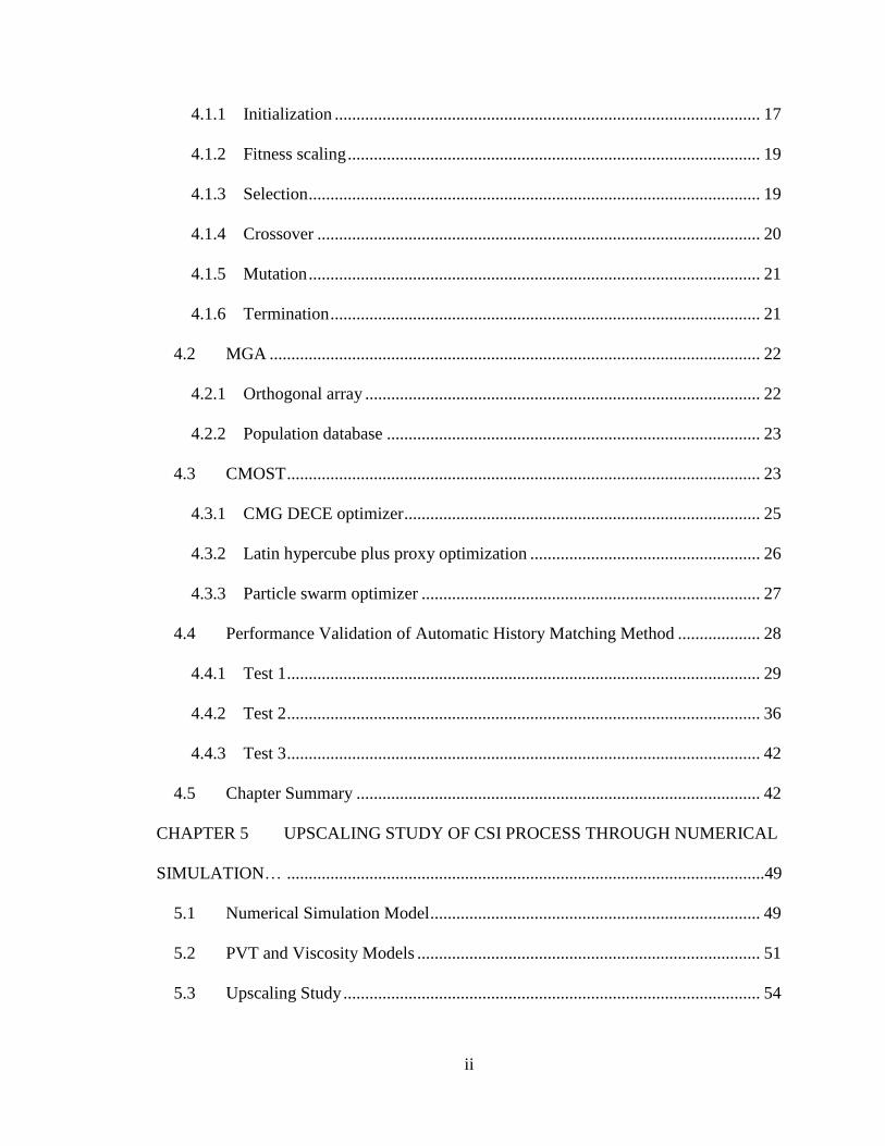
4.1.1 Initialization .................................................................................................. 17
4.1.2 Fitness scaling ............................................................................................... 19
4.1.3 Selection ........................................................................................................ 19
4.1.4 Crossover ...................................................................................................... 20
4.1.5 Mutation ........................................................................................................ 21
4.1.6 Termination ................................................................................................... 21
4.2 MGA ................................................................................................................. 22
4.2.1 Orthogonal array ........................................................................................... 22
4.2.2 Population database ...................................................................................... 23
4.3 CMOST ............................................................................................................. 23
4.3.1 CMG DECE optimizer .................................................................................. 25
4.3.2 Latin hypercube plus proxy optimization ..................................................... 26
4.3.3 Particle swarm optimizer .............................................................................. 27
4.4 Performance Validation of Automatic History Matching Method ................... 28
4.4.1 Test 1 ............................................................................................................. 29
4.4.2 Test 2 ............................................................................................................. 36
4.4.3 Test 3 ............................................................................................................. 42
4.5 Chapter Summary ............................................................................................. 42
CHAPTER 5 UPSCALING STUDY OF CSI PROCESS THROUGH NUMERICAL
SIMULATION… ..............................................................................................................49
5.1 Numerical Simulation Model ............................................................................ 49
5.2 PVT and Viscosity Models ............................................................................... 51
5.3 Upscaling Study ................................................................................................ 54
iii
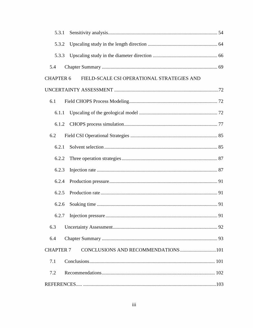
5.3.1 Sensitivity analysis........................................................................................ 54
5.3.2 Upscaling study in the length direction ........................................................ 64
5.3.3 Upscaling study in the diameter direction .................................................... 66
5.4 Chapter Summary ............................................................................................. 69
CHAPTER 6 FIELD-SCALE CSI OPERATIONAL STRATEGIES AND
UNCERTAINTY ASSESSMENT ....................................................................................72
6.1 Field CHOPS Process Modeling ....................................................................... 72
6.1.1 Upscaling of the geological model ............................................................... 72
6.1.2 CHOPS process simulation ........................................................................... 77
6.2 Field CSI Operational Strategies ...................................................................... 85
6.2.1 Solvent selection ........................................................................................... 85
6.2.2 Three operation strategies ............................................................................. 87
6.2.3 Injection rate ................................................................................................. 87
6.2.4 Production pressure ....................................................................................... 91
6.2.5 Production rate .............................................................................................. 91
6.2.6 Soaking time ................................................................................................. 91
6.2.7 Injection pressure .......................................................................................... 91
6.3 Uncertainty Assessment .................................................................................... 92
6.4 Chapter Summary ............................................................................................. 93
CHAPTER 7 CONCLUSIONS AND RECOMMENDATIONS .............................101
7.1 Conclusions ..................................................................................................... 101
7.2 Recommendations ........................................................................................... 102
REFERENCES..... ...........................................................................................................103

iv
APPENDIX A...... ............................................................................................................110
v
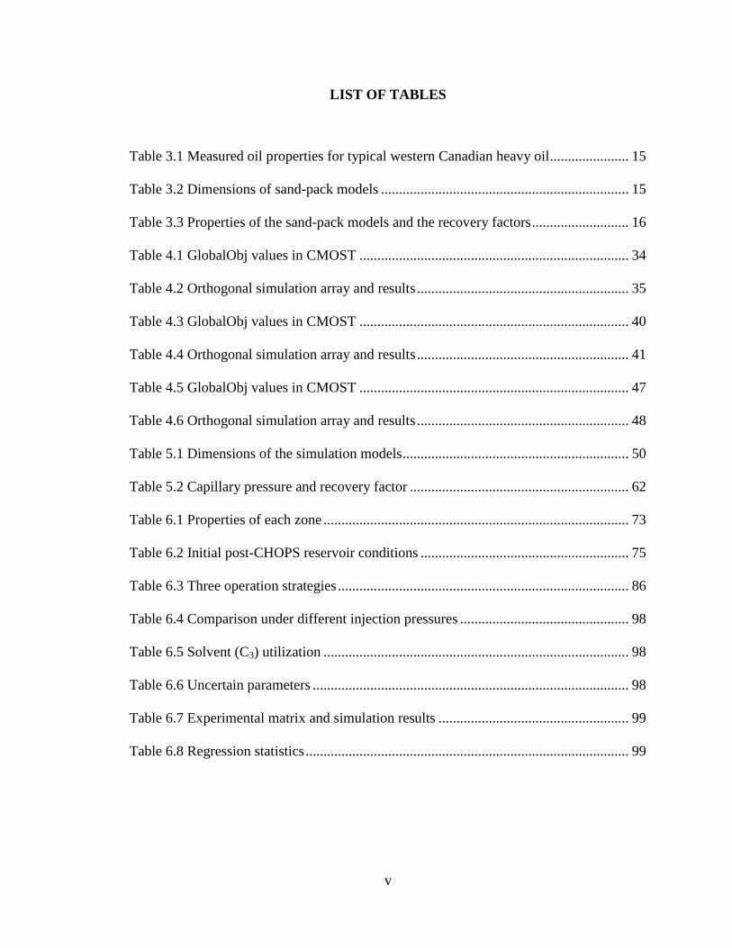
LIST OF TABLES
Table 3.1 Measured oil properties for typical western Canadian heavy oil...................... 15
Table 3.2 Dimensions of sand-pack models ..................................................................... 15
Table 3.3 Properties of the sand-pack models and the recovery factors ........................... 16
Table 4.1 GlobalObj values in CMOST ........................................................................... 34
Table 4.2 Orthogonal simulation array and results ........................................................... 35
Table 4.3 GlobalObj values in CMOST ........................................................................... 40
Table 4.4 Orthogonal simulation array and results ........................................................... 41
Table 4.5 GlobalObj values in CMOST ........................................................................... 47
Table 4.6 Orthogonal simulation array and results ........................................................... 48
Table 5.1 Dimensions of the simulation models ............................................................... 50
Table 5.2 Capillary pressure and recovery factor ............................................................. 62
Table 6.1 Properties of each zone ..................................................................................... 73
Table 6.2 Initial post-CHOPS reservoir conditions .......................................................... 75
Table 6.3 Three operation strategies ................................................................................. 86
Table 6.4 Comparison under different injection pressures ............................................... 98
Table 6.5 Solvent (C3) utilization ..................................................................................... 98
Table 6.6 Uncertain parameters ........................................................................................ 98
Table 6.7 Experimental matrix and simulation results ..................................................... 99
Table 6.8 Regression statistics .......................................................................................... 99
vi
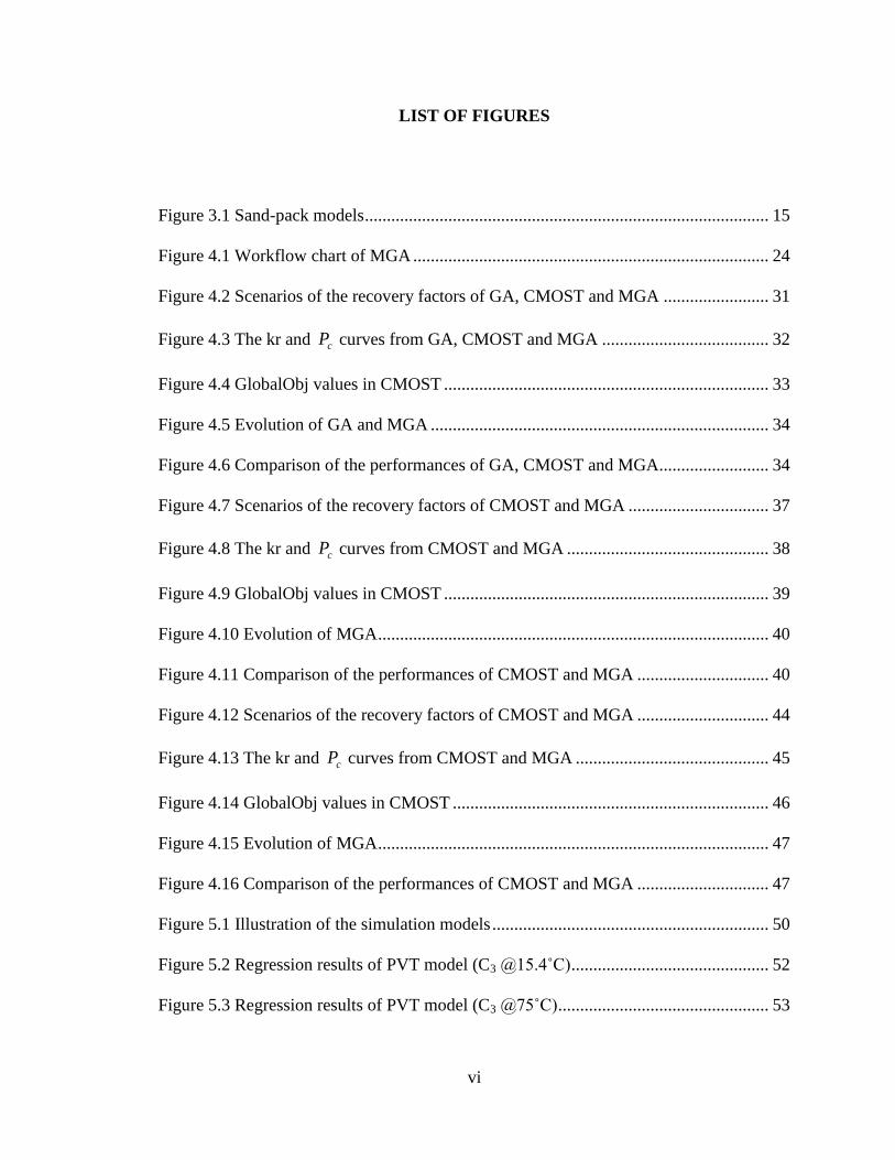
LIST OF FIGURES
Figure 3.1 Sand-pack models ............................................................................................ 15
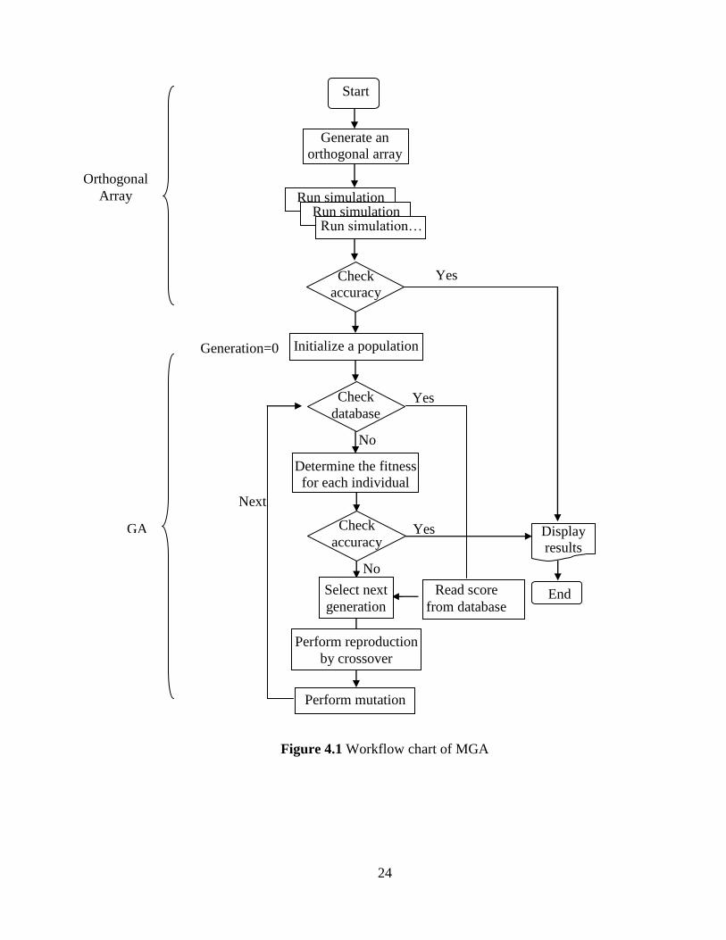
Figure 4.1 Workflow chart of MGA ................................................................................. 24
Figure 4.2 Scenarios of the recovery factors of GA, CMOST and MGA ........................ 31
Figure 4.3 The kr and cP curves from GA, CMOST and MGA ...................................... 32
Figure 4.4 GlobalObj values in CMOST .......................................................................... 33
Figure 4.5 Evolution of GA and MGA ............................................................................. 34
Figure 4.6 Comparison of the performances of GA, CMOST and MGA......................... 34
Figure 4.7 Scenarios of the recovery factors of CMOST and MGA ................................ 37
Figure 4.8 The kr and cP curves from CMOST and MGA .............................................. 38
Figure 4.9 GlobalObj values in CMOST .......................................................................... 39
Figure 4.10 Evolution of MGA ......................................................................................... 40
Figure 4.11 Comparison of the performances of CMOST and MGA .............................. 40
Figure 4.12 Scenarios of the recovery factors of CMOST and MGA .............................. 44
Figure 4.13 The kr and cP curves from CMOST and MGA ............................................ 45
Figure 4.14 GlobalObj values in CMOST ........................................................................ 46
Figure 4.15 Evolution of MGA ......................................................................................... 47
Figure 4.16 Comparison of the performances of CMOST and MGA .............................. 47
Figure 5.1 Illustration of the simulation models ............................................................... 50
Figure 5.2 Regression results of PVT model (C3 @15.4˚C) ............................................. 52
Figure 5.3 Regression results of PVT model (C3 @75˚C) ................................................ 53
vii
Figure 5.4 Model for Test 4 .............................................................................................. 56
Figure 5.5 Liquid-gas relative permeability sets............................................................... 56
Figure 5.6 Effects of relative permeability curves on the CSI process in Test 4 .............. 56
Figure 5.7 Effects of reaction rates on the CSI process in Test 4 ..................................... 58
Figure 5.8 Different grid sizes built by different grid systems ......................................... 58
Figure 5.9 Effects of grid size on the CSI process in Test 8 ............................................. 60
Figure 5.10 Effects of dispersion coefficients on the CSI process in Test 4 .................... 60
Figure 5.11 Capillary curve in Test 4 ............................................................................... 62
Figure 5.12 History matched result of Test 4 ................................................................... 63
Figure 5.13 Models for Tests 5 and 6 ............................................................................... 65
Figure 5.14 History matched results of Tests 5 and 6 ....................................................... 65
Figure 5.15 Capillary pressure curves in Tests 5 and 6 .................................................... 65
Figure 5.16 Final oil saturation distribution of Tests 4, 5 and 6 without cP .................... 67
Figure 5.17 Final oil saturation distribution of Tests 4, 5 and 6 with cP ......................... 67
Figure 5.18 Wormhole locations in Tests 7, 8 and 9 ........................................................ 67
Figure 5.19 History matched results of Tests 7, 8 and 9 ................................................... 67
Figure 5.20 Oil saturation distribution scenarios of experimental models ....................... 68
Figure 5.21 Oil saturation distribution scenarios of simulation models ........................... 68
Figure 5.22 Final oil saturation distribution of Tests 7, 8 and 9 without cP .................... 70
Figure 5.23 Final oil saturation distribution of Test 9 without/ with cP .......................... 70
Figure 5.24 History matched results of Test 9 .................................................................. 71
Figure 6.1 Partial geological model .................................................................................. 74
Figure 6.2 Simulation model............................................................................................. 75
viii
Figure 6.3 Regression results of PVT model (C1+C3 mixture @15.4˚C) ......................... 76
Figure 6.4 Production data of Well V ............................................................................... 78
Figure 6.5 Production data of Well D ............................................................................... 79
Figure 6.6 Wormhole structure ......................................................................................... 83
Figure 6.7 Wormhole structure in the 5th layer ................................................................ 83
Figure 6.8 History matched cumulative oil production of M reservoir ............................ 84
Figure 6.9 History matched cumulative water production of M reservoir ....................... 84
Figure 6.10 The P-T diagram for 0.64C1+0.36C3 at 15.4 C ............................................ 86
Figure 6.11 Oil recovery factors under different operation strategies .............................. 86
Figure 6.12 Oil recovery factors under different injection rates ....................................... 88
Figure 6.13 BHP with different injection rates ................................................................. 89
Figure 6.14 Oil recovery factors under different injection strategies ............................... 90
Figure 6.15 Oil recovery factors under different production pressures ............................ 90
Figure 6.16 Oil recovery factors under different maximum production rates .................. 95
Figure 6.17 Oil recovery factors under different soaking time ......................................... 95
Figure 6.18 The P-T diagrams of different solvent types at 15.4 C ................................ 96
Figure 6.19 Oil recovery factors under different injection pressures ............................... 97
Figure 6.20 Cumulative injection gas under different injection pressures ....................... 97
Figure 6.21 The predicted oil recovery factor of the CSI process .................................... 98
Figure 6.22 Probability distribution of RF for CSI ......................................................... 100
Figure 6.23 Possible range of RF for M reservoir .......................................................... 100
ix
NOMENCLATURE
lS Saturation of the liquid phase
wconS Connate water saturation
orgS Irreducible oil saturation
rogcgk ,rgclk Endpoint values
ogn ,gn Exponents
sim Simulation
exp Experiment
NT Total number of samples
Scale Normalization scale
mY Measured maximum change of recovery factor
Merr Measurement error
i Time point i
n Total number of samples
A Capillary pressure at residual wetting-phase saturation, kPa
cn
Exponent parameter
cp
Capillary pressure, kPa
*
lnS Normalized liquid saturation
Interfacial tension, 10-3
N/m
Contact angle
L Length of wormhole, m

x
xn
Number of wormhole branches
1 Porosity change in open hole caused by sand production
2 Porosity change in dilated zone caused by sand production
Abbreviations
MGA Modified Genetic Algorithm
VAPEX Vapour Extraction
CSI Cyclic Solvent Injection
GA Genetic Algorithm
CMG Computer Modeling Group
EOS Equation of State
RF Recovery Factor
BHP Bottom-hole Pressure
PSO Particle Swarm Optimizer
JST Jossi, Stiel and Thodos Correlation
BPR Back Pressure Regulator
1
CHAPTER 1 INTRODUCTION
1.1 Background
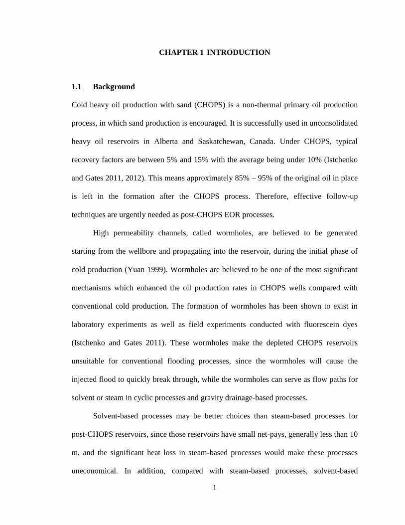
Cold heavy oil production with sand (CHOPS) is a non-thermal primary oil production
process, in which sand production is encouraged. It is successfully used in unconsolidated
heavy oil reservoirs in Alberta and Saskatchewan, Canada. Under CHOPS, typical
recovery factors are between 5% and 15% with the average being under 10% (Istchenko
and Gates 2011, 2012). This means approximately 85% – 95% of the original oil in place
is left in the formation after the CHOPS process. Therefore, effective follow-up
techniques are urgently needed as post-CHOPS EOR processes.
High permeability channels, called wormholes, are believed to be generated
starting from the wellbore and propagating into the reservoir, during the initial phase of
cold production (Yuan 1999). Wormholes are believed to be one of the most significant
mechanisms which enhanced the oil production rates in CHOPS wells compared with
conventional cold production. The formation of wormholes has been shown to exist in
laboratory experiments as well as field experiments conducted with fluorescein dyes
(Istchenko and Gates 2011). These wormholes make the depleted CHOPS reservoirs
unsuitable for conventional flooding processes, since the wormholes will cause the
injected flood to quickly break through, while the wormholes can serve as flow paths for
solvent or steam in cyclic processes and gravity drainage-based processes.
Solvent-based processes may be better choices than steam-based processes for
post-CHOPS reservoirs, since those reservoirs have small net-pays, generally less than 10
m, and the significant heat loss in steam-based processes would make these processes
uneconomical. In addition, compared with steam-based processes, solvent-based
2
processes have many other advantages, such as low energy consumption, less
environmental pollution, in situ upgrading, and lower capital costs (Butler 1991; Jha et al.
1995; Qazvini 2012). In terms of solvent-based processes, several different approaches
including Vapor extraction (VAPEX) (Butler and Mokrys 1989; Butler and Mokrys 1991;
Butler and Mokrys 1993; Jiang 1997; Yazdani and Maini 2005), lateral SVX (Butler and
Jiang 2000), CSI (Ivory et al. 2010) and the Enhanced Cyclic Solvent Process (ECSP) (B.
Yadali Jamaloei et al. 2012), have been proposed in the literature. For the VAPEX
process, the slow mass transfer rate of solvent into the oil phase and lack of gravity in a
thin net-pay reservoir cause the process to have a production rate that is too low to be
economical. For lateral SVX, a continuous solvent injection process, the existence of
wormholes will cause the solvent to break through early, so it is not efficient. However,
for the CSI process, the existence of wormholes can increase the contact area of solvent
and heavy oil, and the wormholes also provide flow channels that allow diluted oil to
flow back to the wellbore. Therefore, CSI is more promising than VAPEX and lateral
SVX as a post-CHOPS enhanced heavy oil recovery method.
The concept of CSI was born from the need to develop a non-thermal process for
thin reservoirs with wormholes. Of course, CSI can also be applied in other reservoirs
where injectivity is sufficiently high. In CSI, a solvent (typically a mixture of propane or
butane with either methane or carbon dioxide) is injected into the reservoir through a
vertical well until the pressure approaches the initial reservoir pressure. The solvent
mixture is selected so that this pressure is close to the dew point of the mixture. Thus, the
solvent has high solubility in the oil but, being in the gas phase, can pressurize the
reservoir without an unacceptable amount of solvent being used, as would be the case if a
3
liquid solvent was injected. Following injection, the solvent is allowed to soak in the
reservoir for a specified period of time. During production, the pressure is drawn down to
about 200 – 500 kPa before the injection period of the next cycle begins. The injection-
soaking-production cycle is repeated a number of times. Dissolution of solvent in the
heavy oil reduces its viscosity and can provide a solution gas drive when the reservoir
pressure is reduced during production. The solvent is selected for a specific reservoir.
The injection and production strategy will be determined based on the existence of water
inflow concerns, pay thickness, reservoir quality and many other conditions.
Reservoir simulation becomes an important tool to select the best development
scheme and also to forecast the oil, gas and water production expected for the field.
Minimizing the difference between the simulation model and the real reservoir is
important to get reliable predicted results. However, limited information on the
geological and geophysical backgrounds of the reservoir is available from well tests,
seismic surveys and logs (Schulze-Riegert et al. 2002). Therefore, the initial reservoir
simulation model needs to be reviewed if the predicted production data from the
simulation model is not as the same as the field production data (Sampaio 2009).
1.2 Problem Statement and Methodology
CSI is the most promising process for a post-CHOPS reservoir (Chang and Ivory 2012).
Experimental studies suggest that oil recovery can reach up to 68% at the lab scale, which
indicates the potential viability of the CSI process. However, CSI is a complex process
and there has been no literature reporting materials on a CSI analytical model. Many
researchers have utilized physical models to study CSI processes (Ivory et al. 2010; Dong
et al. 2012; Du et al. 2013). In the past few years, some researchers have conducted
4
numerical simulation studies on solvent-based processes. One advantage of using
numerical simulation is that it can be used for real, field-scale cases, taking into account
the reservoir heterogeneity, to optimize the operation parameters and evaluate the
economics. The other advantage is that some important information such as the
distribution of viscosity and solvent mole fraction is difficult to measure, but can be
visualized in simulation models. However, upscaling of the CSI process from lab-scale to
field-scale by numerical simulation has not been studied by other researchers.
History matching is a very important process, which is defined by finding a set of
model parameters to minimize the difference between the history production data and the
predicted data, like production pressure and fluid production rates (Schulze-Riegert et al.
2002). History matching can be carried out either manually by reservoir engineers or
automatically by computer. Manual history matching, usually a trial-and-error process, is
difficult and often painstaking because the process behavior is complex and the
parameters to be estimated might be highly interactive (Yang 1991). Also, manual history
matching requires a great deal of experience and depends heavily on personal judgment
and budget. Therefore, automatic history matching is a very attractive tool for estimating
uncertain properties.
In this study, an efficient and effective MGA method was developed to assist the
history matching process and was validated by three CSI tests. In addition, in order to
study the upscaling capability of numerical simulation, another six CSI tests were
conducted under the same or very close conditions with three physical models with
different scales. Based on the experiments, the corresponding numerical model was
established to simulate the experimental tests and upscaling of the CSI process was
5
investigated by numerical simulation. Additionally, the associated uncertainties, such as
relative permeability, reaction rate in the foamy oil model, dispersion coefficient and
capillary pressure, were analyzed. Through comparison of predicted and experimental
results, the capability of predicting scaled-up CSI processes through numerical simulation
was investigated. According to the upscaling study, a typical western Canadian heavy oil
post-CHOPS reservoir (M reservoir) was employed to study the uncertainties (oil relative
permeability, gas relative permeability, capillary pressure and dispersion coefficient)
during the CSI process by numerical simulation.
Through integrating the experimental data, geological data, PVT data and the
reliable numerical simulation models, the upscaling from lab scale to field scale was
completed.
1.3 Thesis Outline
There are seven chapters in this thesis. Chapter 1 describes the background of the CSI
process. The problem statement and research objectives also follow. Chapter 2 is a
comprehensive literature review of the automatic history matching method and previous
experimental and simulation research on the CSI process. Chapter 3 presents the CSI
experimental materials, physical models with different scales and the results of nine CSI
tests. Chapter 4 describes an MGA method, which was validated and compared with the
traditional GA-based history matching method and CMOST with three CSI tests. Chapter
5 describes the upscaling study in the length and diameter directions of the CSI process
through numerical simulation. Chapter 6 provides field-scale CSI operational strategies
and the uncertainty assessment. Lastly, the conclusions and recommendations for future
work are delineated in Chapter 7.
6
CHAPTER 2 LITERATURE REVIEW
2.1 Automatic History Matching Methods
Over the years, a number of history matching algorithms have been proposed. Generally,
these algorithms can be categorized into two groups: 1) gradient-based methods such as
the Gaussian-Newton method (Thomas et al. 1972) and the Levenberg-Marquardt
algorithm (Reynolds et al. 2004); and 2) gradient-free methods including the GA
(Castellini et al. 2005) and simulated annealing (SA) algorithms (Sultan et al. 1994).
In order to obtain the gradient search direction, the gradient of the objective
function is required and can be obtained by using an adjoint equation (Li et al. 2001) or
by computation of the sensitivity coefficient (Tan and Kalogerakis 1992). The gradient-
based algorithms are efficient for problems with a small number of parameters. However,
the computation of the gradient becomes expensive when a model has a large number of
parameters. Moreover, these methods might be stuck in a local optimum and provide a
single solution despite the fact that there are multiple acceptable solutions for the
multidimensional, nonlinear optimization problem. For this kind of problem, the trapping
in a local optimum may be decreased by the use of a global search method (Sun 2005).
Compared to the gradient-based algorithms, gradient-free methods have several
advantages. They have the potential to leave local optima and investigate the global
search space. Their global optimizers show good performance in nonlinear cases and in
complex reservoirs. The variability of models that can equally generate acceptable
solutions for the history matching problem can be qualified. In addition, a global
optimizer will allow a combination of several different types of algorithms, such as a
combination of simulated annealing with genetic algorithms (Silva et al. 2006) or a
7
gradient method with a global optimization method (Schulze-Riegert et al. 2002; Mantica
et al. 2001). However, there are also challenges related to global optimizers. For realistic
applications to history matching, there are no general criteria regarding whether a global
optimum is found. Since optimization algorithms for automatic history matching are
always connected with simulators, global optimization requires a large number of
function calls, which means it requires a large number of simulation runs and substantial
computational effort.
Recently, the GA has been applied frequently in optimization problems. Wathiq
(2013) applied the GA to re-evaluate the optimal wells and net present value (NPV) has
been adopted as an objective function. Tasrief and Kashiwagi (2013) presented an
optimization method based on natural selection, namely a binary-coded GA, to improve
the geometry of a ship. Further information on the theory, applications and importance of
modeling and optimization smart techniques such as the GA, artificial neural networks
(ANN) and particle swarm optimization (PSO), can be found in a variety of chemical and
petroleum engineering processes. Ali et al. (2013) developed a meta-learning algorithm
called least square support vector machine (LSSVM) to predict the compressibility factor
(Z-factor). Aliakbar et al. (2012) applied artificial neural networks as an efficient tool for
the prediction of pure organic compounds’ surface tensions for a wide range of
temperatures. Vasanth Kumar (2009) developed a neural network for predicting
interfacial tension at the crystal/liquid interface. Shafiei et al. (2013) developed a new
screening tool based on ANN optimized with PSO to assess the performance of
steamflooding in naturally fractured carbonate reservoirs.
8
In this study, the GA, as a global search method, is chosen to assist automatic
computational cost. In order to improve the computational efficiency, an orthogonal array
and a population database were incorporated with the GA to enhance the quality of the
running cases and save the running time by decreasing the total running cases.
2.2 Experimental Study on the CSI Process
Investigations of the solvent-based cyclic production processes are limited to those by
Lim et al. (1995; 1996), Dong et al. (2006), Cuthiell et al. (2006), Ivory et al. (2010) and
Jamaloei et al. (2012). In their studies, the cyclic solvent injection process consisted of
three periods: a solvent injection period, a soaking period, and the production period.
Dong et al. (2006) mentioned that applying the pressure-cycling process with methane
injection involves the restoring of the solution gas drive that provided primary
production. Ivory et al. (2010) conducted an experiment, which consisted of primary
production and six solvent injection cycles, to evaluate the performance of a 28% C3H8 -
72% CO2 solvent mixture in the CSI process. The injection time was very long (62 – 80
days), and production lasted about 22 days. The recovery factor after six cycles was about
50%. It indicated that the CSI process shows great potential as a post-cold production
process.
Jamaloei et al. (2012) proposed using methane as a chase gas in the solvent
injection period during the CSI process and their results showed the oil recovery factor
can be significantly improved by using propane as a solvent and methane as chasing gas,
compared to using methane only. Du (2013) conducted a series of experimental
investigations of the effects of wormholes on the CSI process.
9
Dong et al. performed an experimental study about cyclic solvent injection. Their
study included two parts, methane cyclic solvent process (CSP) and methane and propane
mixed solvent enhanced cyclic solvent process (ECSP). Their performance for heavy oil
recovery was investigated by conducting a series of experiments in sand-pack saturated
with crude oil and brine. In order to examine the behavior of methane CSP, the
experimental results of oil recovery factor, ultimate oil recovery, oil recovery rate,
pressure profiles during repressurization, soaking and production and drawdown rate in
the 6 cycles are presented and analyzed. In the ECSP part, methane and propane are
injected in two separate slugs cyclically. Methane is used to provide solution-gas drive
energy and most of the propane is dissolved in the oil to keep a low oil viscosity. A series
of six ECSP cycles was conducted in the same sand-pack. The experimental results of the
six ECSP cycles are compared to those of the six methane CSP cycles. This comparison
indicates that ECSP effectively has the advantage of the viscosity reduction and solvent-
gas-drive mechanisms during the early time of the production cycles.
It is widely believed that a network of high permeability channels is created in the
reservoir during the CHOPS process. The wormholes definitely would affect the CSI
process if the CSI process was introduced after the CHOPS process. Although the
performance of CSI is mainly affected by the wormholes, current experimental work did
not consider the contribution of wormholes on the performance of CSI. Also, for solvent-
based enhanced heavy oil recovery processes, it is very important to investigate their
performance at different scales, so that the performance of these processes in the field
scale can be better predicted. Therefore, it is necessary to conduct an experimental study
10
to investigate the performance of the CSI process under the effect of wormholes with
physical models with different scales.
Du et al. investigated the effect of wormholes on the CSI process. In their study, a
series of experimental tests was conducted by using three cylindrical sand-pack models
with different geometries to investigate the effect of wormhole properties on the post-
CHOPS CSI process. The effect of wormhole length, the wormhole’s vertical location in
the model, model diameter, model length, and model orientation on the performance of
CSI process is discussed. The experimental results suggest that the existence of a
wormhole can significantly increase the oil production rate. The larger the wormhole
coverage is, the better is the CSI performance. A reservoir or well with wormholes
developed at the bottom is more favorable for the post-CHOPS CSI process. The model
length hardly affected the oil production rate compared to the wormhole length. A well
with a horizontal wormhole is inclined to get a good CSI performance. The results are of
importance for understanding the CSI performance under the effect of wormholes and
upscaling study.
2.3 Simulation Study on the CSI Process
Ivory et al. (2010) developed a numerical simulation model for history matching their
radial drainage experiment. In order to simulate the CSI process, they determined the
conditions (fluid saturation and pressure distributions) first in the model at the end of
primary production. This was accomplished using a gas exsolution model. In this model,
a total of three oil-phase components and one gas-phase component were used. In
developing the CSI numerical simulation model, the non-equilibrium representation of
solvent solubility, solvent/oil mixture viscosities and the mixing parameters of the
11
process (diffusion and dispersion) were incorporated into the reservoir fluid model. In the
model, the delay in a gaseous component dissolving or exsolving from the oil depends on
the difference between its current concentration in the oil phase and its equilibrium
concentration in the oil phase, as determined from its concentration in the gas phase, and
its temperature and pressure.
Chang and Ivory (2012) conducted a field-scale numerical simulation study for the
CSI process and concluded that the oil recovery from CSI is mainly dominated by the
wormholes created during CHOPS. They proposed a numerical model that uses “mass
transfer” rate equations to represent non-equilibrium solvent solubility behavior in field-
scale simulations of CSI. The model contains mechanisms to consider foaming or ignore
it depending on the field behavior. It has been used to match laboratory experiments,
design CSI operating strategies, and interpret CSI field pilot results. The paper also
summarizes the impact on simulation predictions of post-CHOPS reservoir
characterizations where the wormhole region was represented by one of five
configurations. The impacts of grid size, upscaling, well inflow parameter, solvent
dissolution and exsolution rate constants, and injection strategy were also examined. In
Xu’s upscaling work (2012), different scales of physical modeling were required in order
to reduce the uncertainties in predicting the field-scale VAPEX performance. For
VAPEX, analytical models and correlations have been developed to scale up oil
production rates from lab-scale to field prediction (Butler and Mokrys 1989; Das and
Butler 1998; Boustani and Maini 2001; Karmaker and Maini 2003; Yazidani and Maini
2005; Kapadia et al. 2006; Nenniger and Dunn 2008). Compared to analytical models,
numerical models have greater potential to be used as scale up methods for the VAPEX
12
process due to the improved prediction results, applicability to real field cases, and
availability of property visualization.
The simulation results indicated that: (1) oil recovery from CSI is mostly limited to
high permeability regions created during CHOPS; (2) compared to fine grid blocks, the
use of coarse grid blocks in effective permeability model simulations resulted in a much
quicker reduction in bottom-hole pressure (BHP) during production and much lower oil
rates as a result of rapid reservoir depressurization. One needs to adjust the parameter to
compensate for this behavior if using coarse grid blocks; (3) changing the frequency
factors for gas exsolution and/or dissolution and /or changing the dispersion coefficient
values is an effective upscaling strategy; and (4) a single cycle should not be used to
estimate solvent recovery as it will be low due to an unrecoverable (by pressure reduction
alone) solvent inventory being built up in the part of the reservoir to where the solvent
penetrates. In later cycles, a greater percentage of the injected solvent is recovered as the
total solvent retention at the end of each cycle only increases a relatively small amount.
2.4 Chapter Summary
From the literature review, it can be seen that an efficient and effective automatic history
matching method is necessary for the CSI process. The experimental study on the CSI
process shows that the CSI process has great potential to recover heavy oil. In the last
several years, Ivory, Dong and Du did a series of CSI tests from different aspects. From
the simulation point of view, Chang did a field-scale CSI simulation study. The upscaling
study of the CSI process from lab-scale to field-scale is very important.
13
CHAPTER 3 CSI EXPERIMENTS
In this study, nine CSI tests conducted by Du et al. (2013, 2014) were used to evaluate
the performance of an MGA method and study the upscaling of the CSI process. A brief
description and summary of these CSI tests are presented in this chapter.
3.1 Experimental Section
In this experimental study, a typical heavy oil sample was employed, the properties of
which are listed in Table 3.1. Propane, with a purity of 99.99 wt % (Praxair), was used as
the solvent. In order to keep the solvent in the gas phase and to achieve its maximum
solubility in the heavy oil, the propane was injected at 800 kPa (below its dew point
pressure) at room temperature (21 ˚C). In general, the sand-pack will have a porosity of
33% – 36% and a permeability of 5 – 6 Darcy. Constant connate water saturation, based
on experimental measurements, was also assumed with no movable water content.
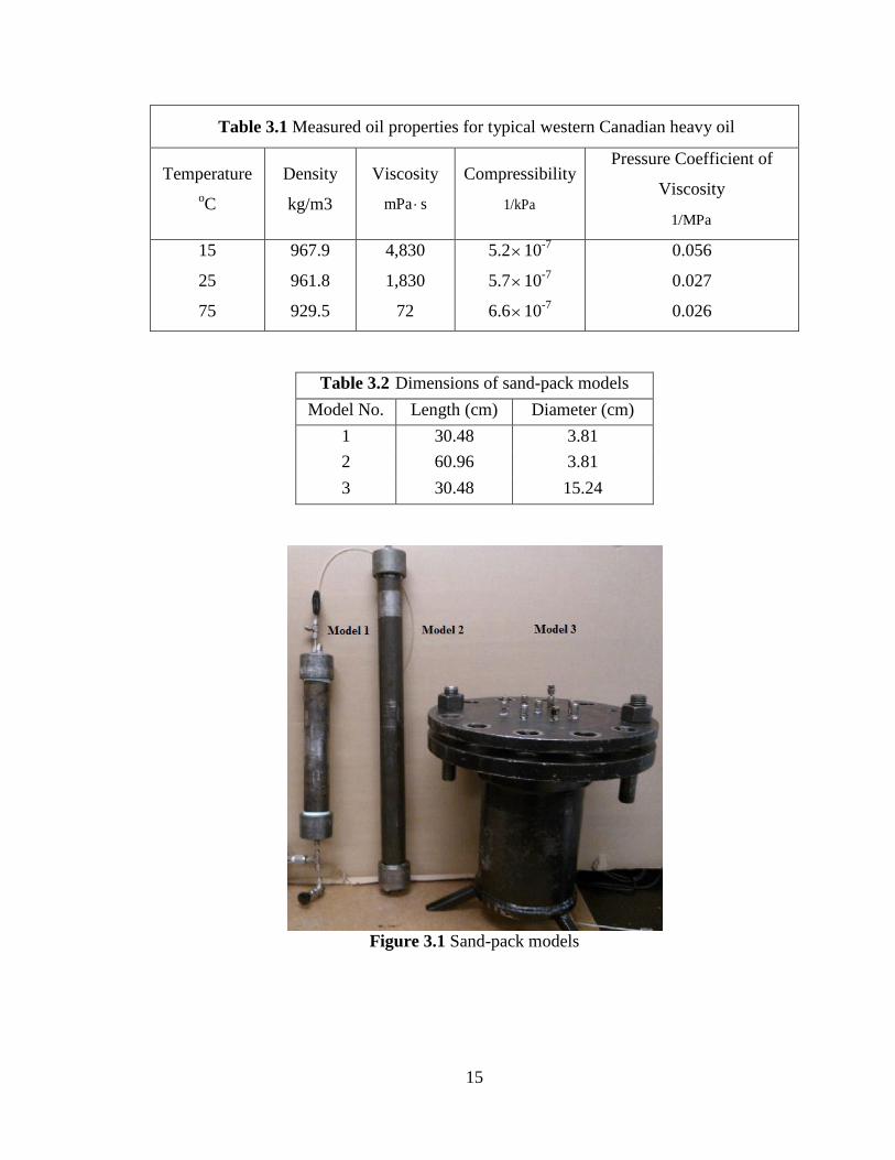
In order to study the performance of the CSI process at different scales and
provide data for upscaling analysis, three cylindrical sand-pack models were used. The
dimensions of these three sand-pack models are listed in Table 3.2. Model 1, which has a
length of 30.48 cm and a diameter of 3.81 cm, serves as a base model. Model 2, with a
diameter the same as that of Model 1, is doubled in length to upscale the base model in
the length direction. Model 3, with a length the same as that of Model 1, has a diameter
four times that of the base model to upscale the base model in the diameter direction.
Figure 3.1 shows the three sand-pack models. These models were set horizontally with
both injector and producer on the left side, with a mimic wormhole. In summary, each
cycle includes a 45-minute injecting period, 10-minute soaking period and unfixed
production period. The sand-pack pressure reached the desired pressure after a 45-minute
14
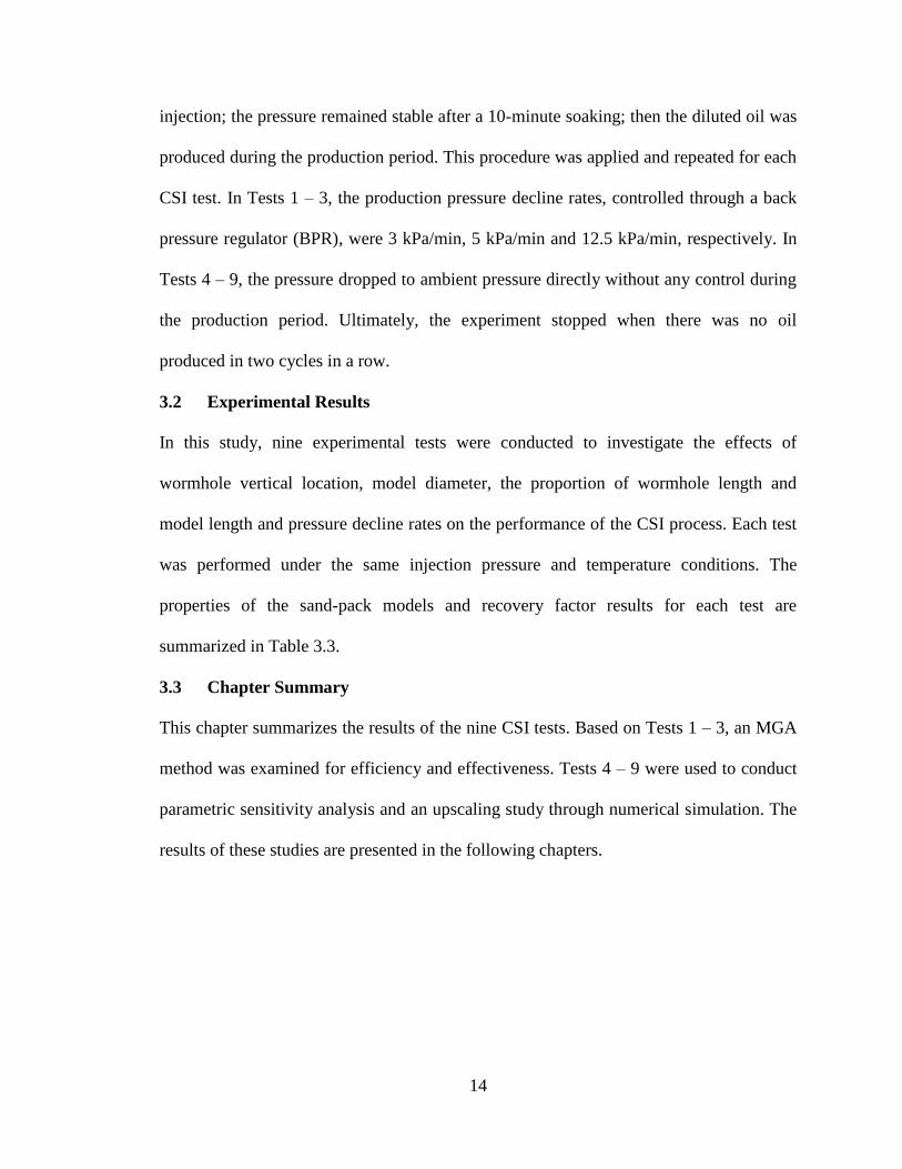
injection; the pressure remained stable after a 10-minute soaking; then the diluted oil was
produced during the production period. This procedure was applied and repeated for each
CSI test. In Tests 1 – 3, the production pressure decline rates, controlled through a back
pressure regulator (BPR), were 3 kPa/min, 5 kPa/min and 12.5 kPa/min, respectively. In
Tests 4 – 9, the pressure dropped to ambient pressure directly without any control during
the production period. Ultimately, the experiment stopped when there was no oil
produced in two cycles in a row.
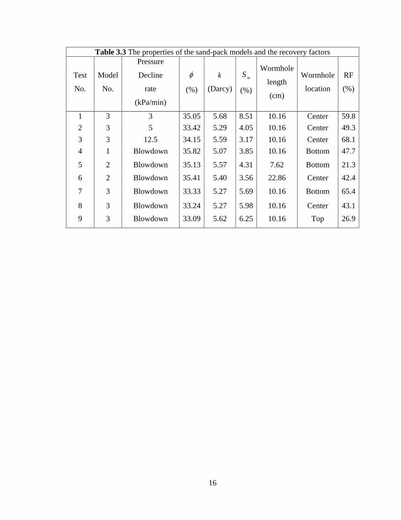
3.2 Experimental Results
In this study, nine experimental tests were conducted to investigate the effects of
wormhole vertical location, model diameter, the proportion of wormhole length and
model length and pressure decline rates on the performance of the CSI process. Each test
was performed under the same injection pressure and temperature conditions. The
properties of the sand-pack models and recovery factor results for each test are
summarized in Table 3.3.
3.3 Chapter Summary
This chapter summarizes the results of the nine CSI tests. Based on Tests 1 – 3, an MGA
method was examined for efficiency and effectiveness. Tests 4 – 9 were used to conduct
parametric sensitivity analysis and an upscaling study through numerical simulation. The
results of these studies are presented in the following chapters.
15
Table 3.1 Measured oil properties for typical western Canadian heavy oil
Temperature
oC
Density
kg/m3
Viscosity
smPa
Compressibility
1/kPa
Pressure Coefficient of
Viscosity
1/MPa
15
25
75
967.9
961.8
929.5
4,830
1,830
72
5.210-7
5.710-7
6.610-7
0.056
0.027
0.026
Table 3.2 Dimensions of sand-pack models
Model No. Length (cm) Diameter (cm)
1 30.48 3.81
2 60.96 3.81
3 30.48 15.24
Figure 3.1 Sand-pack models
16
Table 3.3 The properties of the sand-pack models and the recovery factors
Test
No.
Model
No.
Pressure
Decline
rate
(kPa/min)
(%)
k
(Darcy)
wS
(%)
Wormhole
length
(cm)
Wormhole
location
RF
(%)
1 3 3 35.05 5.68 8.51 10.16 Center 59.8
2 3 5 33.42 5.29 4.05 10.16 Center 49.3
3 3 12.5 34.15 5.59 3.17 10.16 Center 68.1
4 1 Blowdown 35.82 5.07 3.85 10.16 Bottom 47.7
5 2 Blowdown 35.13 5.57 4.31 7.62 Bottom 21.3
6 2 Blowdown 35.41 5.40 3.56 22.86 Center 42.4
7 3 Blowdown 33.33 5.27 5.69 10.16 Bottom 65.4
8 3 Blowdown 33.24 5.27 5.98 10.16 Center 43.1
9 3 Blowdown 33.09 5.62 6.25 10.16 Top 26.9
17
CHAPTER 4 A MODIFIED GA-BASED HISTORY MATCHING METHOD
In this chapter, an MGA method is proposed to history match the CSI experiments. This
optimization algorithm has the following two key steps:
1. Orthogonal array design: The purpose of orthogonal array design is to construct
combinations of the input parameter values so that the maximum information can be
obtained from the minimum number of simulation runs. In this step, an optimal initial
population (one set of parameters) will be obtained.
2. GA optimization: Several external programs will modify the executive file, call
the CMG automatically, and evaluate the results. Simultaneously, the GA toolbox in
Matlab® will keep generating the next new population by the operation of selection,
crossover and mutation.
4.1 GA
The GA is a stochastic global search and optimization method that mimics the metaphor
of natural biological evolution (J. Holland 1975). The evolution usually starts with an
initial population composed of randomly generated individuals. In each generation, the
fitness of every individual in the population is evaluated by the value of the objective
function in the optimization problem. The fitter individuals are selected from the current
population, and each individual's genome is modified to form a new generation by
crossover and mutation. The new generation of candidate solutions is then used in the
next iteration of the algorithm. Commonly, the algorithm terminates when either a
satisfactory fitness level has been reached for the population, or a maximum number of
generations has been produced.
4.1.1 Initialization
18
Usually, a set of initial populations is chosen randomly from the search space. The
population size can significantly affect the performance of the GA. If the population is
too small, it is not likely to find a good solution for the problem at hand. Increasing the
population size enables the genetic algorithm to search more points in the search space
and thereby, obtain better results. However, if the population is too large, the GA will
waste time processing unnecessary individuals, and this might result in an unacceptably
slow performance. It is suggested that the population size is at least the same value as the
number of variables (Grefenstette 1986). In view of the high computational cost of the
CSI simulation, the initial population size was set at 10.
In this study, the liquid-gas relative permeability curve and the capillary pressure
are two important and sensitive parameters in the CSI process. The Corey correlation, the
most widely used functional representation of the relative permeability and capillary
pressure curves, was applied in the history matching.
The liquid-gas relative permeability and capillary pressure curves can be expressed
as:
ogn
orgwcon
orgwconl
rogcgrog )SS1
SSS(kk
(4.1)
gn
orgwcon
lrgclrg )
SS1
S1(kk
(4.2)
cn
orgwcon
orgwconl
cSS1
SSS1AP
(4.3)
where lS is the saturation of the liquid phase; wconS is the connate water saturation; orgS
is the irreducible oil saturation; rogcgk and
rgclk are the endpoint values; and ogn and
gn are
the corresponding exponents. cP is the capillary pressure and cn is the corresponding

19
exponent. Therefore, for the Corey model,rgclk ,
gn , rogcgk ,
ogn , A , cn are considered in
the history matching process.
4.1.2 Fitness scaling
After a population is initialized, the fitness value for each member of the current
population is computed. The fitness function converts the raw score of the objective
function into a value in a range that is suitable for the selection function because the
range of fitness scores will affect the performance of the GA. If the range is large, an
individual with a high score could be reproduced quickly, which leads to a limited search
space and fast convergence. In contrast, if the fitness scores do not change much, the
chances of reproducing the individuals are almost the same. As a result, the search will
progress slowly. Possible fitness scaling functions include the rank, proportional, and
shift linear scales. In this study, the rank scale is used so that the individuals are ranked
based on the raw score of each individual. The fittest individual is ranked as one, the next
fittest is two, and so on. The advantage of this method is that the effect of the spread of
the raw scores can be removed.
4.1.3 Selection
The selection rules choose parents for the next generation based on their scaled values
from the fitness function. An individual can be selected more than once as a parent, in
which case it contributes its genes to more than one child. The selection process has to be
balanced: a selection that is too strong means that suboptimal-fit individuals will take
over the population, and thereby reduce the diversity needed for further change. On the
other hand, a selection that is too weak results in slow evolution (Mitchell 1996). The
selection functions include the stochastic uniform, remainder, roulette, and tournament
20
functions. The roulette function simulates a roulette wheel with the area of each segment
proportional to its expectation. The algorithm then uses a random number to select one of
the sections with a probability equal to its area. The remainder function assigns parents
deterministically from the integer part of each individual's scaled value and then uses
roulette selection on the remaining fractional part. The stochastic uniform function lays
out a line in which each parent corresponds to a section of the line of a length
proportional to its expectation. The algorithm moves along the line in steps of equal size,
one step for each parent. At each step, the algorithm allocates a parent from the section it
lands on. The tournament function selects each parent by choosing individuals at random,
and then choosing the best individual out of a set to be a parent. In this study, the
stochastic uniform selection method was used as the selection strategy.
4.1.4 Crossover
The crossover operator combines two individuals or parents in the current generation to
form a new individual or child for the next generation. The crossover operator functions
include scattered crossover, single-point crossover, two-point crossover, intermediate
crossover, and arithmetic crossover. The single-point crossover function chooses a
random integer n between one and the number of variables. Then, the vector entries
numbered less than or equal to n from the first parent are selected, and genes numbered
greater than n from the second parent are selected. Thus, a new chromosome is generated
by combining the selected genes from the two parents. In the two-point crossover
function, two positions are chosen at random, and the segments between them are
exchanged. The scattered crossover function creates a random binary vector, which then
selects the genes where the vector is a one from the first parent and the genes where the
21
vector is a zero from the second parent and combines the genes to form the child. The
intermediate crossover function creates children by a weighted average of the parents and
it is controlled by a single parameter. (Chipperfield et al. 1994) The arithmetic crossover
creates children that are the weighted arithmetic mean of two parents. In this study, the
single-point crossover method was adopted. The advantage of this method is that some
good patterns will not be damaged easily due to the crossover.
4.1.5 Mutation
The mutation operator creates a child by applying random changes to a single individual
in the current generation, which provides genetic diversity and enables the GA to search a
broader space. The mutation operator includes the functions of Gaussian, uniform, and
adaptive feasible mutation. In the Gaussian mutation function, random numbers are taken
from a Gaussian distribution centered on zero. The uniform mutation function involves a
two-step process and only part of the individual is selected for mutation with a certain
mutation rate, which is replaced by a random number selected uniformly. However, since
these two functions are applicable to the unconstrained problem, the adaptive feasible
mutation function was used in this work because of the studied constraint problem. This
method randomly generates directions that are adaptive with respect to the last successful
or unsuccessful generation and a step length is chosen along each direction so that linear
constraints and bounds are satisfied.
4.1.6 Termination
Stopping criteria determine what causes the algorithm to terminate. This optimization
process can be terminated by setting conditions related to the following factors:
22
(1) The maximum number of generations: the algorithm stops when the maximum
number of generations is reached.
(2) Fitness limit: the algorithm stops when the value of the fitness function for the
best point in the current population is less than or equal to the fitness limit.
4.2 MGA
Recently, the GA has been applied frequently in the optimization problems. Wathiq
(2013) applied it to re-evaluate the optimal wells and net present value (NPV) has been
adopted as an objective function. Tasrief and Kashiwagi (2013) presented an optimization
method based on natural selection, namely a binary-coded GA, to improve the geometry
of a ship. Since the optimization algorithms in automatic history matching are always
connected with simulators, global optimization requires a large number of function calls,
which means it requires a large number of simulation runs and substantial computational
effort.
In this section, an MGA method is developed. In order to improve the
computational efficiency, an orthogonal array and a population database were
incorporated with the GA to enhance the quality of the running cases and save the
running time by decreasing the total running cases. Figure 4.1 shows the logic flow for
this MGA method. The optimization modules and the interaction between the commercial
simulator STARS® and the optimization modules were programmed by MATLAB,
shown in Appendix A.
4.2.1 Orthogonal array
As the initial population greatly affects the performance of the GA, an orthogonal
simulation array will be run in order to obtain a good initial population.
23
An orthogonal array is chosen because it can handle several input parameters
with certain levels. It is useful when the number of inputs to the system is relatively
small, but too large to allow for exhaustive testing of every possible input to the systems.
In this study, L25 (5^6), a 25 run design used to estimate the main effects from a 5-level,
6-factor design, was chosen to build the orthogonal simulation array. The multiple
inferences were covered as much as possible. The oil recovery factor was selected as the
response variable.
4.2.2 Population database
As each individual needs to be calculated, a population database is read first to check
whether there is a matching record in the database. The precision of the match can be set
in the program. If a matching record is found, the fitness score is read directly from the
population database; if it is not, the external program is invoked and the calculated fitness
score will be recorded into the database with the corresponding individual. This process
ensures the computation time will be minimized. Also, this database is useful if the
execution process is interrupted accidentally, in which case, it is not necessary to restart
the optimization from the beginning and the scores can simply be read directly from the
database.
4.3 CMOST
CMOST is the CMG’s history matching, optimization, sensitivity analysis, and
uncertainty assessment tool. It may be used in any situation where a user runs multiple
simulation jobs with the intention of either converging on a better solution to some
problem or seeing the effect of input parameter changes on output properties. Once a job
Has been created by CMOST, it will automatically submit simulation jobs and check
24
Figure 4.1 Workflow chart of MGA
Generation=0
Check
database
Display
results
Next
Yes
No
Yes
Start
End
Check
accuracy Yes
No
Check
accuracy
Generate an
orthogonal array
Initialize a population
Determine the fitness
for each individual
Select next
generation
Perform reproduction
by crossover
Perform mutation
Read score
from database
Run simulation Run simulation
Run simulation…
Orthogonal
Array
GA
25
their status periodically. Once simulations have been completed, CMOST will
automatically process the results. It will then visualize the results in ways that will
provide insight into the problem.
History matching with CMOST provides an effective and efficient way to match
simulation results to production history. CMOST can automatically create multiple
derived simulation datasets from the Master Dataset by varying selected dataset
parameters and then running the simulation jobs. As jobs are completed, CMOST will
analyze the results to determine how well they match the production history. An
optimizer will then be used to determine parameter values for new simulation jobs. As
more simulations are completed, the results will converge to multiple optimal solutions
which provide satisfactory history matching if user specified parameters and their ranges
are appropriate.
In this study, the variables related to the liquid-gas relative permeability and
capillary pressure curves were considered as the parameters in the CMOST history
matching process. The CMG DECE optimizer, Latin hypercube plus proxy optimization
and particle swarm optimizer in CMOST were evaluated as the optimization methods.
4.3.1 CMG DECE optimizer
The CMG DECE Optimizer implements the CMG’s proprietary optimization method:
Designed Exploration and Controlled Evolution. The DECE optimization method tries to
imitate the process which reservoir engineers commonly use to solve history matching or
optimization problems. For simplicity, DECE optimization can be described as an
iterative optimization process that applies the designed exploration stage and the
controlled evolution stage sequentially. In the designed exploration stage, the goal is to
26
explore the search space in a designed random manner such that maximum information
about the solution space can be obtained. In this stage, experimental design and Tabu
search techniques are applied to pick parameter values and create representative
simulation datasets. In the controlled evolution stage, statistical analyses are performed
for the simulation results obtained in the designed exploration stage. Based on the
analyses, the DECE algorithm scrutinizes every candidate value of each parameter and
determines whether there is a better chance to improve solution quality if certain
candidate values are rejected. These rejected candidate values are remembered by the
algorithm and they will not be used in the next controlled exploration stage. To minimize
the possibility of being trapped in local minima, the DECE algorithm checks rejected
candidate values from time to time to make sure previous rejection decisions are still
valid. If the algorithm determines that certain rejection decisions are not valid, the
rejection decisions are recalled and the corresponding candidate values will be used
again. The results demonstrate that the DECE optimization method is reliable and
efficient. Therefore, it is one of the recommended optimization methods in CMOST.
4.3.2 Latin hypercube plus proxy optimization
This optimization algorithm has the following four key steps:
1. Latin hypercube design: The purpose of the Latin hypercube design is to
construct combinations of the input parameter values so that the maximum information
can be obtained from the minimum number of simulation runs.
2. Proxy modeling: In this step, an empirical proxy model is built by using the
training data obtained from Latin hypercube design runs. It is many orders of magnitude
faster than the actual simulation.
27
3. Proxy-based optimization: Due to the intrinsic limitations of proxy models, it is
generally believed that they usually cannot give accurate predictions. Therefore, the
optimal solution obtained based on the proxy model may not be the true optimal solution
for the actual reservoir model. In order to find the true optimal solution, a pre-defined
number of suboptimal solutions of the proxy model, one of which could be the optimum
solution, are generated to increase the chance of finding the global optimum solution.
4. Validation and iteration: A series of reservoir simulations need to be run for
each possible optimum solution, in order to obtain their true objective function values.
After that, these solutions can be added to the initial training data set to further improve
the prediction accuracy of the proxy model. With the new proxy model, a new set of
possible optimum solutions can be obtained. This iteration procedure can be continued
for a given number of iterations or until a satisfactory optimal solution is found.
4.3.3 Particle swarm optimizer
The PSO is a population based stochastic optimization technique. Social influences and
learning enable a person to maintain cognitive consistency. People solve problems by
talking with other people, and as they interact their beliefs, attitudes, and behaviors
change; the changes could typically be depicted as the individuals moving toward one
another in a sociocognitive space. The particle swarm simulates this kind of social
optimization. The system is initialized with a population of random solutions and
searches for optima by updating generations. The individuals iteratively evaluate their
candidate solutions and remember the location of their best success so far, making this
information available to their neighbors; they are also able to see where their neighbors
28
have had success. Movements through the search space are guided by these successes,
with the population converging towards good solutions.
4.4 Performance Validation of Automatic History Matching Method
The performance of the MGA method was validated in terms of effectiveness. In this
section, three CSI tests, conducted in the lab, were used to validate the performance of
the MGA method from the point of view of accuracy.
In manual history matching, the variations between the simulation results and
measured production data are usually taken into account by the reservoir engineer
intuitively and qualitatively. In computer-assisted history matching, a quantitative
approach should be used to account for the data quality (Yang et al. 2007). The history
matching accuracy was evaluated by calculating the GlobalObj, which was used to
measure the relative difference between the simulation results and measured production
data, which is defined as Equation 4.4:
%1001
exp
Scale
NT
RFRF
GlobalObj
n
i
i
sim
i
(4.4)
where RF represents the oil recovery factor; the superscripts sim and exp represent the
simulated and experimental quantities, respectively; the subscript i represents the value
at time point i ; NT is the total number of samples; and Scale is the normalization scale.
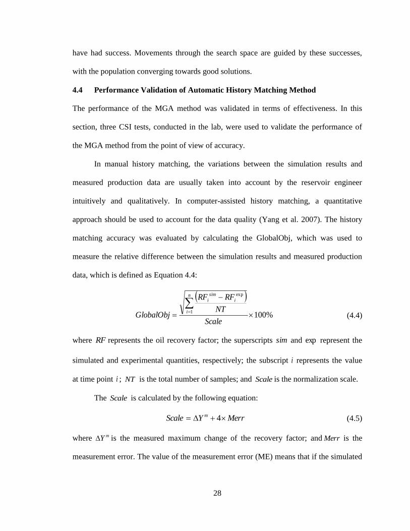
The Scale is calculated by the following equation:
MerrYScale m 4 (4.5)
where mY is the measured maximum change of the recovery factor; and Merr is the
measurement error. The value of the measurement error (ME) means that if the simulated
29
result is between (historical value - ME) and (historical value + ME), the matching is
considered to be satisfactory.
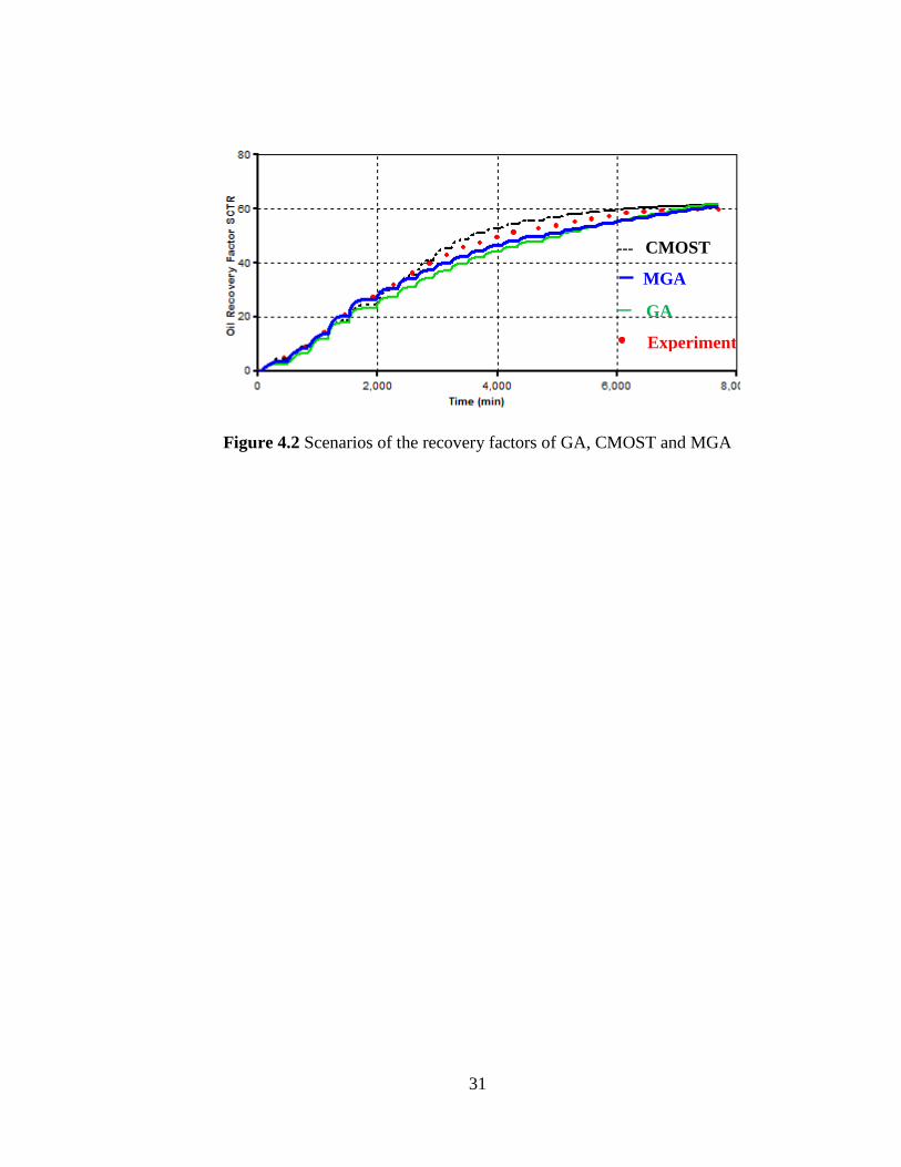
4.4.1 Test 1
The pressure decline rate in Test 1 was controlled by 3 kPa/min in the production period.
The connate water saturation and residual oil saturation in Test 1 were 8.51% and 1%,
respectively. Because of the nature of history matching problems, multiple solutions
could be obtained with different methods. Therefore, all the results of the history
matching from the GA, MGA and CMOST are very close to the experimental result in
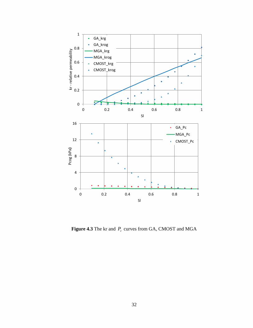
Figure 4.2, whereas the liquid-gas relative permeability curves and capillary pressure
curves obtained from these three methods are very different, as shown in Figure 4.3.
Additionally, the gas relative permeability curves are all quite low, prompting foamy oil
behavior to occur in CSI.
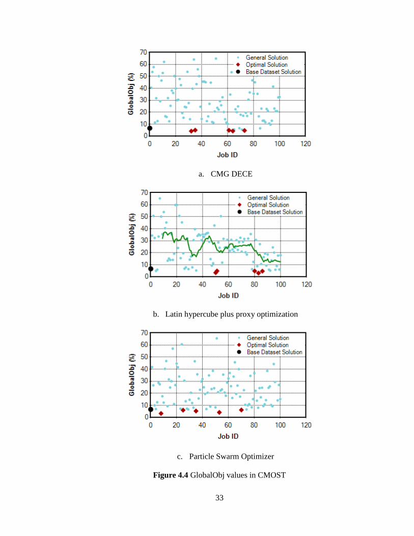
In CMOST, the CMG DECE optimizer, Latin hypercube plus proxy optimizer and
particle swarm optimizer were applied and 100 cases were run for each method. Figure
4.4 and Table 4.2 show the GlobalObj values of the best five optimal solutions for each
method obtained by CMOST. The Latin hypercube plus proxy optimizer obtained the
lowest GlobalObj value, 3.141.
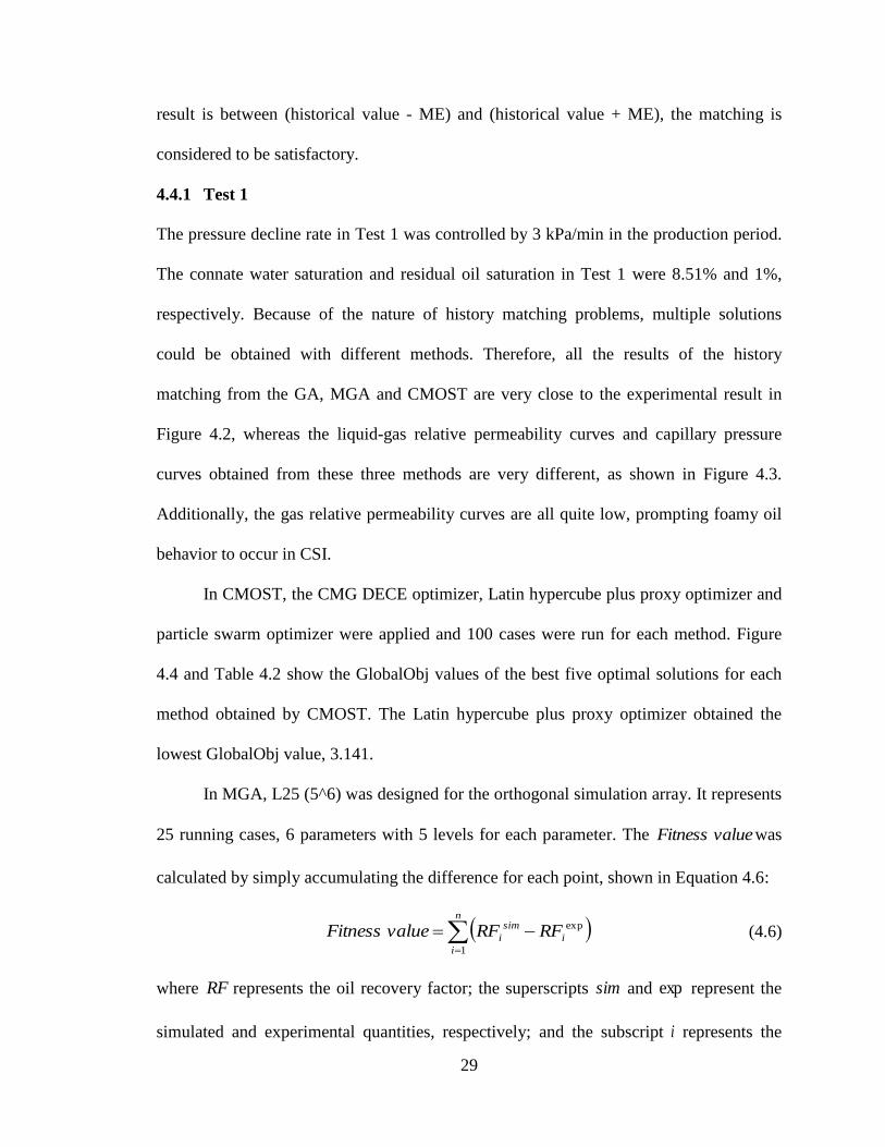
In MGA, L25 (5^6) was designed for the orthogonal simulation array. It represents
25 running cases, 6 parameters with 5 levels for each parameter. The valueFitness was
calculated by simply accumulating the difference for each point, shown in Equation 4.6:
n
i
i
sim
i RFRFvalueFitness1
exp (4.6)
where RF represents the oil recovery factor; the superscripts sim and exp represent the
simulated and experimental quantities, respectively; and the subscript i represents the
30
value at time point i . The orthogonal simulation array and the fitness values are shown in
Table 4.1. Run 14 obtained the minimum valueFitness , so the corresponding
parameters ([0.05, 4, 0.1, 2, 20, 1]) were set as the initial population in the following
MGA procedure. In addition, as well as in CMOST, 100 simulation runs were conducted
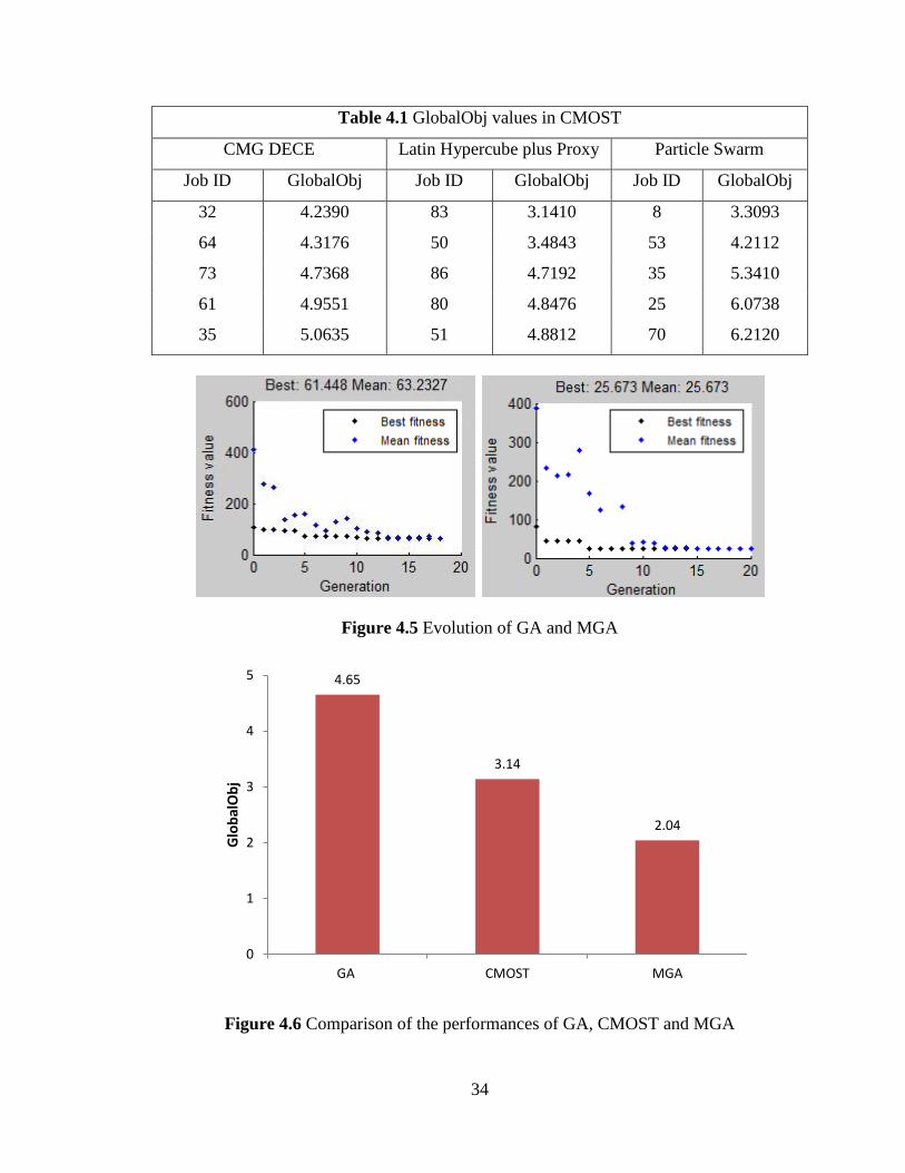
for the GA and MGA. Figure 4.5 shows the evolution of the generations for the GA and
MGA. Because of the existence of the population database, nearly 75% individuals’
results were obtained directly from the database, avoiding unnecessary repeated running
cases. Therefore, the CPU time for running 100 cases was significantly reduced from 41
hours with the GA to 11 hours with the MGA by using a Dell® computer with 4 cores and
a processor base frequency of 3.00 GHz.
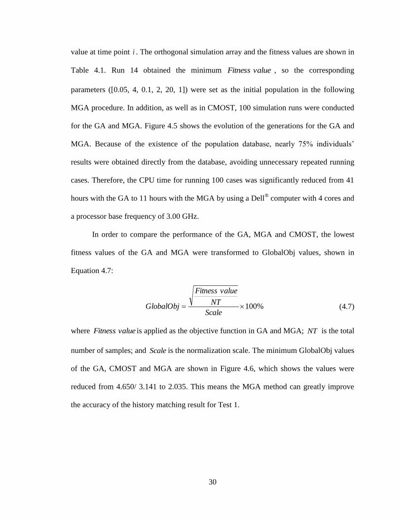
In order to compare the performance of the GA, MGA and CMOST, the lowest
fitness values of the GA and MGA were transformed to GlobalObj values, shown in
Equation 4.7:
%100Scale
NT
valueFitness
GlobalObj (4.7)
where valueFitness is applied as the objective function in GA and MGA; NT is the total
number of samples; and Scale is the normalization scale. The minimum GlobalObj values
of the GA, CMOST and MGA are shown in Figure 4.6, which shows the values were
reduced from 4.650/ 3.141 to 2.035. This means the MGA method can greatly improve
the accuracy of the history matching result for Test 1.
31
Figure 4.2 Scenarios of the recovery factors of GA, CMOST and MGA
--- CMOST
MGA
- GA
Experiment
32
Figure 4.3 The kr and cP curves from GA, CMOST and MGA
0
0.2
0.4
0.6
0.8
1
0 0.2 0.4 0.6 0.8 1
kr -
rel
ativ
e p
erm
eab
ility
Sl
GA_krg
GA_krog
MGA_krg
MGA_krog
CMOST_krg
CMOST_krog
0
4
8
12
16
0 0.2 0.4 0.6 0.8 1
Pco
g (k
Pa)
Sl
GA_Pc
MGA_Pc
CMOST_Pc
33
a. CMG DECE
b. Latin hypercube plus proxy optimization
c. Particle Swarm Optimizer
Figure 4.4 GlobalObj values in CMOST
34
Table 4.1 GlobalObj values in CMOST
CMG DECE Latin Hypercube plus Proxy Particle Swarm
Job ID GlobalObj Job ID GlobalObj Job ID GlobalObj
32 4.2390 83 3.1410 8 3.3093
64 4.3176 50 3.4843 53 4.2112
73 4.7368 86 4.7192 35 5.3410
61 4.9551 80 4.8476 25 6.0738
35 5.0635 51 4.8812 70 6.2120
Figure 4.5 Evolution of GA and MGA
Figure 4.6 Comparison of the performances of GA, CMOST and MGA
4.65
3.14
2.04
0
1
2
3
4
5
GA CMOST MGA
Glo
bal
Ob
j

35
Table 4.2 Orthogonal simulation array and results
rgclk gn
rogcgk ogn A cn RF valueFitness
Run 1 0.01 0.5 0.1 0.5 0 0.5 11.98 878.4
Run 2 0.01 1 0.3 1 5 1 56.16 94.2
Run 3 0.01 2 0.5 2 10 2 81.58 365.0
Run 4 0.01 4 0.7 4 15 3 49.27 126.2
Run 5 0.01 8 0.9 8 20 4 26.65 479.5
Run 6 0.03 0.5 0.3 2 15 4 36.13 536.0
Run 7 0.03 1 0.5 4 20 0.5 65.00 150.7
Run 8 0.03 2 0.7 8 0 1 25.07 659.2
Run 9 0.03 4 0.9 0.5 5 2 93.42 810.5
Run 10 0.03 8 0.1 1 10 3 64.28 170.0
Run 11 0.05 0.5 0.5 8 5 3 24.65 675.5
Run 12 0.05 1 0.7 0.5 10 4 2.01 1002.7
Run 13 0.05 2 0.9 1 15 0.5 91.76 758.6
Run 14 0.05 4 0.1 2 20 1 58.15 48.6
Run 15 0.05 8 0.3 4 0 2 35.06 349.8
Run 16 0.07 0.5 0.7 1 20 2 73.18 237.9
Run 17 0.07 1 0.9 2 0 3 33.75 463.6
Run 18 0.07 2 0.1 4 5 4 11.78 881.6
Run 19 0.07 4 0.3 8 10 0.5 33.56 413.5
Run 20 0.07 8 0.5 0.5 15 2 92.93 855.9
Run 21 0.09 0.5 0.9 4 10 1 55.84 173.9
Run 22 0.09 1 0.1 8 15 2 11.97 890.1
Run 23 0.09 2 0.3 0.5 20 3 73.02 190.3
Run 24 0.09 4 0.5 1 0 4 42.33 327.6
Run 25 0.09 8 0.7 2 5 0.5 60.19 186.7
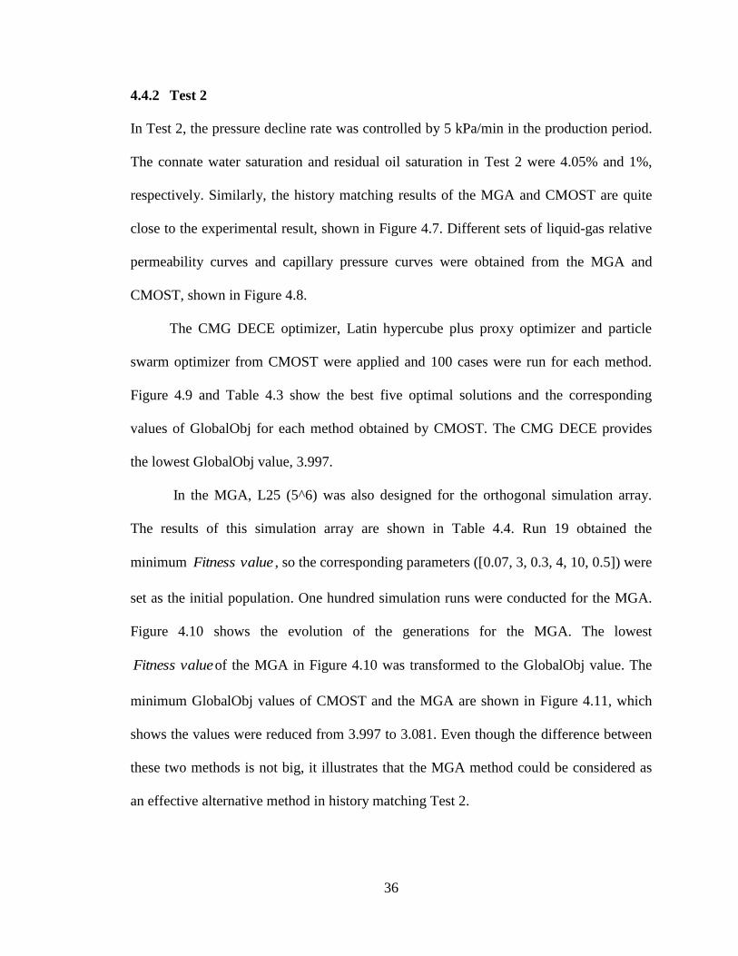
36
4.4.2 Test 2
In Test 2, the pressure decline rate was controlled by 5 kPa/min in the production period.
The connate water saturation and residual oil saturation in Test 2 were 4.05% and 1%,
respectively. Similarly, the history matching results of the MGA and CMOST are quite
close to the experimental result, shown in Figure 4.7. Different sets of liquid-gas relative
permeability curves and capillary pressure curves were obtained from the MGA and
CMOST, shown in Figure 4.8.
The CMG DECE optimizer, Latin hypercube plus proxy optimizer and particle
swarm optimizer from CMOST were applied and 100 cases were run for each method.
Figure 4.9 and Table 4.3 show the best five optimal solutions and the corresponding
values of GlobalObj for each method obtained by CMOST. The CMG DECE provides
the lowest GlobalObj value, 3.997.
In the MGA, L25 (5^6) was also designed for the orthogonal simulation array.
The results of this simulation array are shown in Table 4.4. Run 19 obtained the
minimum valueFitness , so the corresponding parameters ([0.07, 3, 0.3, 4, 10, 0.5]) were
set as the initial population. One hundred simulation runs were conducted for the MGA.
Figure 4.10 shows the evolution of the generations for the MGA. The lowest
valueFitness of the MGA in Figure 4.10 was transformed to the GlobalObj value. The
minimum GlobalObj values of CMOST and the MGA are shown in Figure 4.11, which
shows the values were reduced from 3.997 to 3.081. Even though the difference between
these two methods is not big, it illustrates that the MGA method could be considered as
an effective alternative method in history matching Test 2.
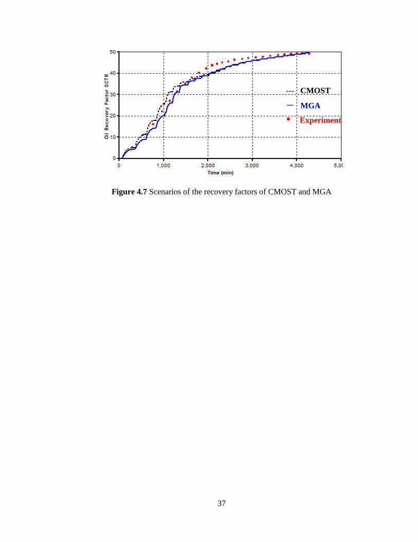
37
Figure 4.7 Scenarios of the recovery factors of CMOST and MGA
--- CMOST
- MGA
Experiment
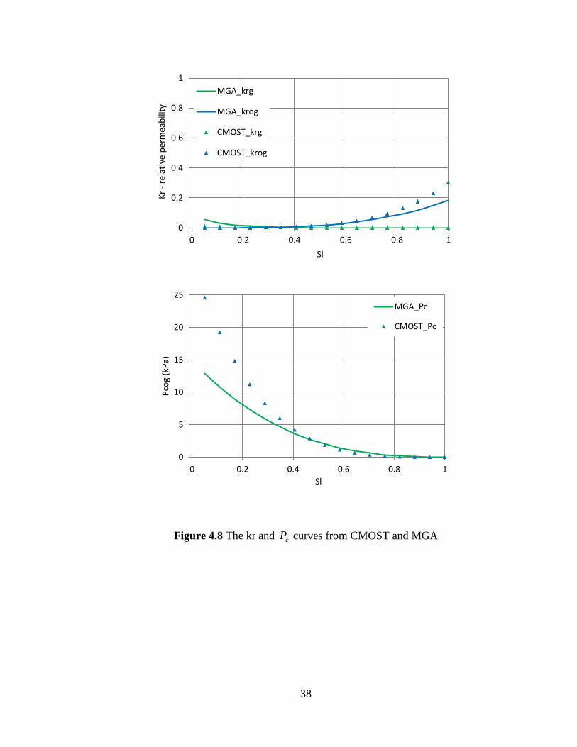
38
Figure 4.8 The kr and cP curves from CMOST and MGA
0
0.2
0.4
0.6
0.8
1
0 0.2 0.4 0.6 0.8 1
Kr
- re
lati
ve p
erm
eab
ility
Sl
MGA_krg
MGA_krog
CMOST_krg
CMOST_krog
0
5
10
15
20
25
0 0.2 0.4 0.6 0.8 1
Pco
g (k
Pa)
Sl
MGA_Pc
CMOST_Pc
39
a. CMG DECE
b. Latin hypercube plus proxy optimization
c. Particle Swarm Optimizer
Figure 4.9 GlobalObj values in CMOST
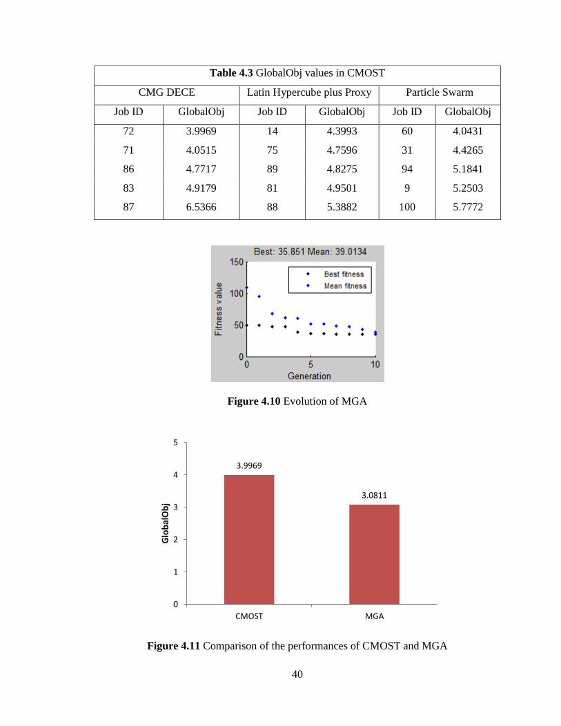
40
Table 4.3 GlobalObj values in CMOST
CMG DECE Latin Hypercube plus Proxy Particle Swarm
Job ID GlobalObj Job ID GlobalObj Job ID GlobalObj
72 3.9969 14 4.3993 60 4.0431
71 4.0515 75 4.7596 31 4.4265
86 4.7717 89 4.8275 94 5.1841
83 4.9179 81 4.9501 9 5.2503
87 6.5366 88 5.3882 100 5.7772
Figure 4.10 Evolution of MGA
Figure 4.11 Comparison of the performances of CMOST and MGA
3.9969
3.0811
0
1
2
3
4
5
CMOST MGA
Glo
bal
Ob
j
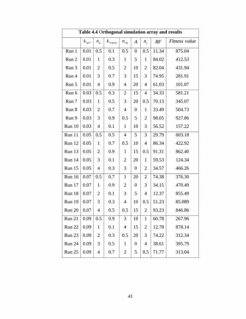
41
Table 4.4 Orthogonal simulation array and results
rgclk gn
rogcgk ogn A cn RF valueFitness
Run 1 0.01 0.5 0.1 0.5 0 0.5 11.34 875.04
Run 2 0.01 1 0.3 1 5 1 84.02 412.53
Run 3 0.01 2 0.5 2 10 2 82.04 431.94
Run 4 0.01 3 0.7 3 15 3 74.95 281.91
Run 5 0.01 4 0.9 4 20 4 61.03 101.07
Run 6 0.03 0.5 0.3 2 15 4 34.33 581.21
Run 7 0.03 1 0.5 3 20 0.5 70.13 345.07
Run 8 0.03 2 0.7 4 0 1 33.49 504.73
Run 9 0.03 3 0.9 0.5 5 2 98.05 927.86
Run 10 0.03 4 0.1 1 10 3 56.52 157.22
Run 11 0.05 0.5 0.5 4 5 3 29.79 603.18
Run 12 0.05 1 0.7 0.5 10 4 86.34 422.92
Run 13 0.05 2 0.9 1 15 0.5 91.31 862.40
Run 14 0.05 3 0.1 2 20 1 59.53 124.34
Run 15 0.05 4 0.3 3 0 2 34.57 466.26
Run 16 0.07 0.5 0.7 1 20 2 74.38 376.30
Run 17 0.07 1 0.9 2 0 3 34.15 470.49
Run 18 0.07 2 0.1 3 5 4 12.37 855.49
Run 19 0.07 3 0.3 4 10 0.5 51.23 85.089
Run 20 0.07 4 0.5 0.5 15 2 93.23 846.86
Run 21 0.09 0.5 0.9 3 10 1 60.78 267.96
Run 22 0.09 1 0.1 4 15 2 12.78 878.14
Run 23 0.09 2 0.3 0.5 20 3 74.22 312.34
Run 24 0.09 3 0.5 1 0 4 38.61 395.79
Run 25 0.09 4 0.7 2 5 0.5 71.77 313.04
42
4.4.3 Test 3
The pressure decline rate in Test 3 was controlled by 12.5 kPa/min in the production
period. The connate water saturation and residual oil saturation in Test 3 were 3.17% and
1%, respectively. The results of the history matching are shown in Figure 4.12. The
liquid-gas relative permeability and capillary pressure curves obtained from the MGA
and CMOST are vastly different, as shown in Figure 4.13. As indicated before, the gas
relative permeability curves are quite low, prompting foamy oil behavior to occur in CSI.
Similarly, the CMG DECE optimizer, Latin hypercube plus the proxy optimizer
and particle swarm optimizer in CMOST were applied and 100 cases were run for each
method. Figure 4.14 and Table 4.6 show the best five optimal solutions and the
corresponding values of GlobalObj for each method obtained by CMOST. The particle
swarm optimizer gave the lowest GlobalObj value, 2.656.
In the MGA, the same as Tests 1 and 2, L25 (5^6) were used to design the
orthogonal simulation array. The results of this simulation array are shown in Table 4.5.
The minimum valueFitness with the parameters ([0.03, 0.5, 0.3, 2, 15, 4]) were obtained
from Run 6. After obtaining the initial population, 100 simulation runs were conducted
for the MGA. Figure 4.10 shows the evolution of the generations for the MGA. The
lowest valueFitness from the MGA in Figure 4.15 was calculated and then transformed
to the GlobalObj value. The minimum GlobalObj values of the MGA and CMOST are
shown in Figure 4.16. It can be seen that the value was reduced from 2.656 to 1.647,
which means the MGA method could greatly improve the accuracy of the history
matching result in Test 3.
4.5 Chapter Summary
43
In this chapter, an MGA method was developed by integrating a population database and
orthogonal array with the GA to improve the effectiveness of the algorithm. This MGA
method was validated by history matching three sets of CSI experiments. The running
efficiency was significantly enhanced by the existence of a population database with the
MGA method compared to that of the GA method. In addition, the accuracy of history
matching, evaluated by the minimum value of GlobalObj, was improved with the MGA
method, compared with that obtained by CMOST. Thus, the proposed automatic history
matching method is very effective in history matching CSI tests.
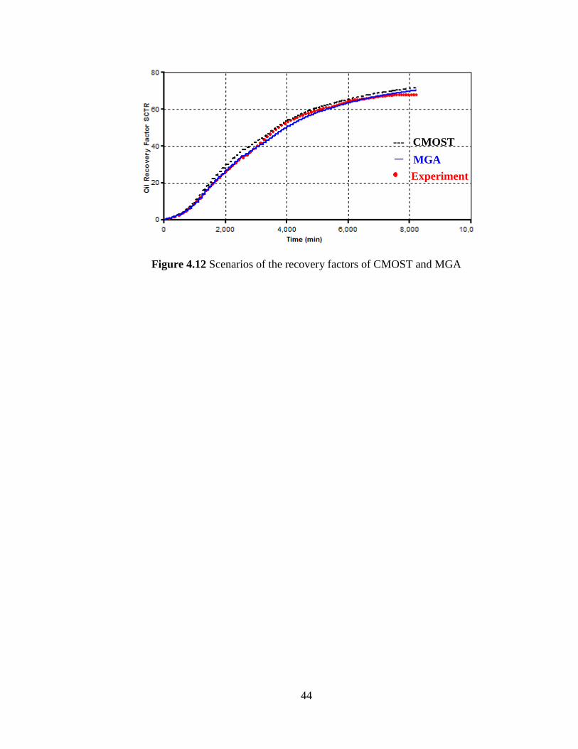
44
Figure 4.12 Scenarios of the recovery factors of CMOST and MGA
--- CMOST
- MGA
Experiment
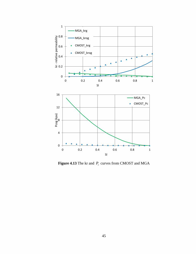
45
Figure 4.13 The kr and cP curves from CMOST and MGA
0
0.2
0.4
0.6
0.8
1
0 0.2 0.4 0.6 0.8 1
kr -
rel
ativ
e p
erm
eab
ility
Sl
MGA_krg
MGA_krog
CMOST_krg
CMOST_krog
0
4
8
12
16
0 0.2 0.4 0.6 0.8 1
Pco
g (k
pa)
Sl
MGA_Pc
CMOST_Pc
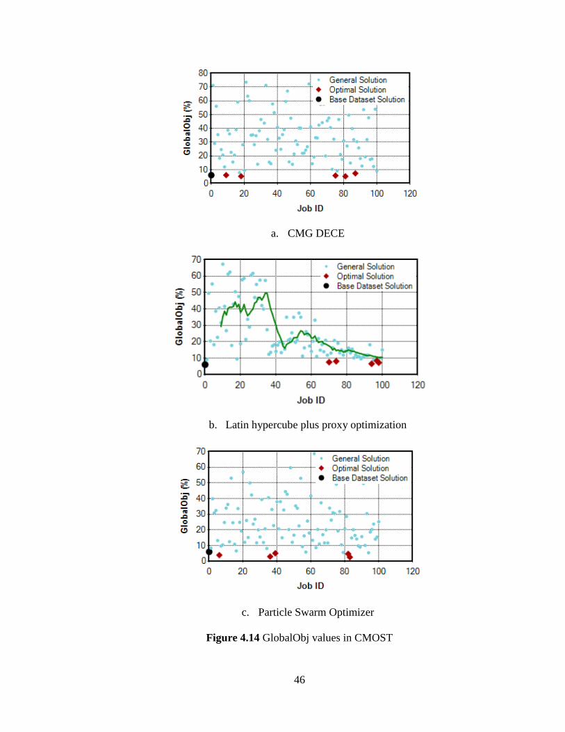
46
a. CMG DECE
b. Latin hypercube plus proxy optimization
c. Particle Swarm Optimizer
Figure 4.14 GlobalObj values in CMOST
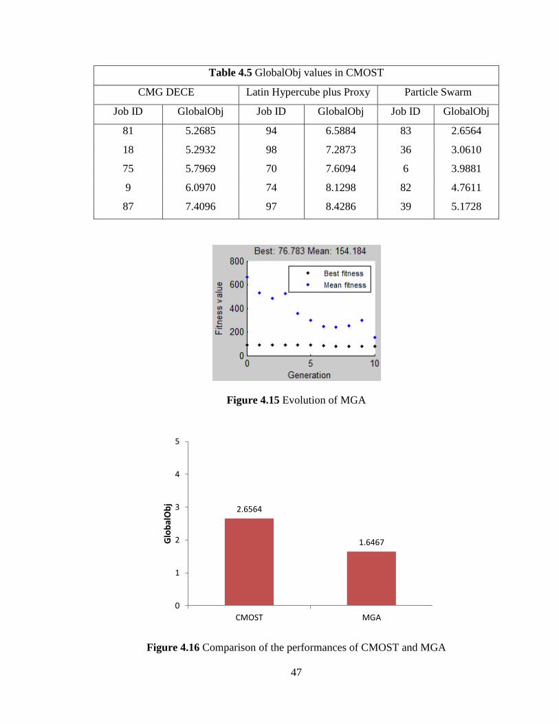
47
Table 4.5 GlobalObj values in CMOST
CMG DECE Latin Hypercube plus Proxy Particle Swarm
Job ID GlobalObj Job ID GlobalObj Job ID GlobalObj
81 5.2685 94 6.5884 83 2.6564
18 5.2932 98 7.2873 36 3.0610
75 5.7969 70 7.6094 6 3.9881
9 6.0970 74 8.1298 82 4.7611
87 7.4096 97 8.4286 39 5.1728
Figure 4.15 Evolution of MGA
Figure 4.16 Comparison of the performances of CMOST and MGA
2.6564
1.6467
0
1
2
3
4
5
CMOST MGA
Glo
bal
Ob
j
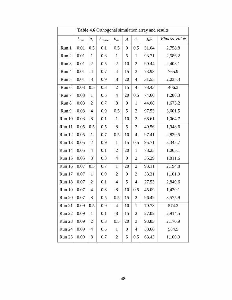
48
Table 4.6 Orthogonal simulation array and results
rgclk gn
rogcgk ogn A cn RF valueFitness
Run 1 0.01 0.5 0.1 0.5 0 0.5 31.04 2,758.8
Run 2 0.01 1 0.3 1 5 1 93.71 2,586.2
Run 3 0.01 2 0.5 2 10 2 90.44 2,403.1
Run 4 0.01 4 0.7 4 15 3 73.93 765.9
Run 5 0.01 8 0.9 8 20 4 31.55 2,035.3
Run 6 0.03 0.5 0.3 2 15 4 78.43 406.3
Run 7 0.03 1 0.5 4 20 0.5 74.60 1,288.3
Run 8 0.03 2 0.7 8 0 1 44.08 1,675.2
Run 9 0.03 4 0.9 0.5 5 2 97.53 3,601.5
Run 10 0.03 8 0.1 1 10 3 68.61 1,064.7
Run 11 0.05 0.5 0.5 8 5 3 40.56 1,948.6
Run 12 0.05 1 0.7 0.5 10 4 97.41 2,829.5
Run 13 0.05 2 0.9 1 15 0.5 95.71 3,345.7
Run 14 0.05 4 0.1 2 20 1 78.25 1,065.1
Run 15 0.05 8 0.3 4 0 2 35.29 1,811.6
Run 16 0.07 0.5 0.7 1 20 2 93.11 2,194.8
Run 17 0.07 1 0.9 2 0 3 53.31 1,101.9
Run 18 0.07 2 0.1 4 5 4 27.53 2,840.6
Run 19 0.07 4 0.3 8 10 0.5 45.09 1,420.1
Run 20 0.07 8 0.5 0.5 15 2 96.42 3,575.9
Run 21 0.09 0.5 0.9 4 10 1 70.73 574.2
Run 22 0.09 1 0.1 8 15 2 27.02 2,914.5
Run 23 0.09 2 0.3 0.5 20 3 93.83 2,170.9
Run 24 0.09 4 0.5 1 0 4 58.66 584.5
Run 25 0.09 8 0.7 2 5 0.5 63.43 1,100.9
49
CHAPTER 5 UPSCALING STUDY OF CSI PROCESS THROUGH NUMERICAL
SIMULATION
In this chapter, several CSI simulation models were constructed by the CMG STARS
based on laboratory experiments, and corresponding phase behavior (PVT) and viscosity
models were also built by the CMG WinProp®. By perturbing the parameters of the
simulation model, the impact of these parameters on CSI performance was investigated,
and the upscaling study was also conducted in the length and diameter directions,
respectively.
5.1 Numerical Simulation Model
Prior to implementing the CSI process at the field scale, an extensive simulation and
feasibility study is needed in addition to the experimental observations. Numerical
simulation was used to link all the experimental data in order to reach conclusions. In
view of this, the semi-compositional module STARS, a commercially available simulator
developed by the CMG, was employed to simulate the experiments. Because all the tests
were conducted with the models set horizontally, an orthogonal grid system was applied
for the cylindrical homogeneous models, as shown in Figure 5.1. The dimensions of the
simulation models are shown in Table 5.1. The injector and producer were both located at
the left side of these models. Pure propane was used as the solvent, injected near its
saturation pressure of 800 kPa at room temperature (21oC). The sand-pack models were
assumed to be uniform in the CSI experiments. Therefore, in each test, a constant
porosity and permeability distribution in all directions and constant connate water
saturation were set in the numerical models, according to the experimental
measurements.
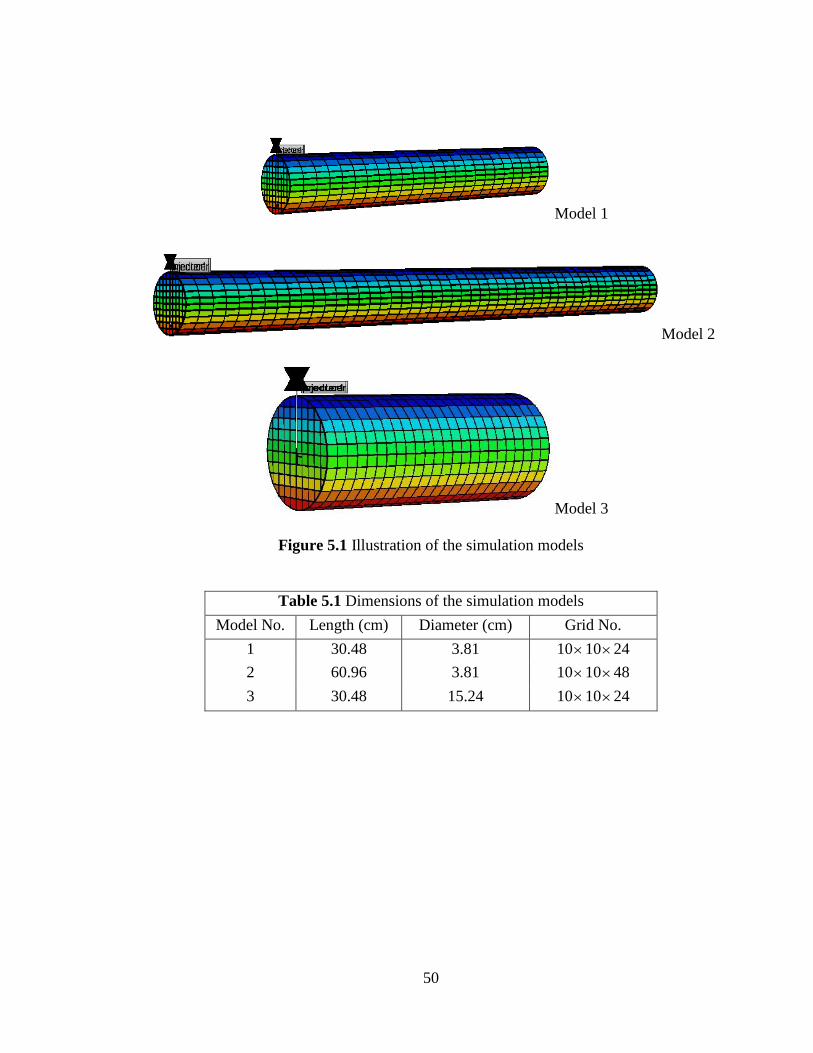
50
Model 1
Model 2
Model 3
Figure 5.1 Illustration of the simulation models
Table 5.1 Dimensions of the simulation models
Model No. Length (cm) Diameter (cm) Grid No.
1 30.48 3.81 101024
2 60.96 3.81 101048
3 30.48 15.24 101024
51
5.2 PVT and Viscosity Models
The tuned PVT and viscosity models for every specific solvent/oil system are extremely
important for solvent-based processes, as they directly influence the amount of solvent
dissolved into the oil phase and consequently determine the mobility of the diluted oil.
The general, available correlations and PVT models will most likely lead to seriously
unreliable conclusions. Experience has shown that simply applying existing correlations
or theories, without calibrating the models to match actual lab data, provides inaccurate
predictions (Ali Yazdani and Brij B. Maini 2009). The interactions of the hydrocarbon
components with injected solvent are specific for every oil/solvent system and need to be
accurately modeled and verified by experimentally measured data. Therefore, in this
study, the equation of state (EOS) was tuned by the experimental PVT data.
Currently, there are two types of viscosity correlation available in WinProp: the
Jossi, Stiel and Thodos (JST) correlation and the Pedersen corresponding states
correlation. The viscosities of the liquid and vapor phases are calculated with the same
correlation. The JST method depends very strongly on the density of the mixture
predicted by the EOS. Thus, use of the JST correlation may result in serious errors if the
phase densities are incorrect. It is recommended that the EOS be tuned to match
volumetric data before attempting to predict or match viscosities with the JST correlation.
While the Pedersen correlation is not dependent on having accurate density predictions,
the JST technique is. Moreover, the Pedersen correlation is expected to give better liquid
viscosity predictions for light and medium gravity oils than the JST model (WinProp
User’s Guide). Therefore, the viscosity model was constructed by the Modified Pedersen
Model in this study.
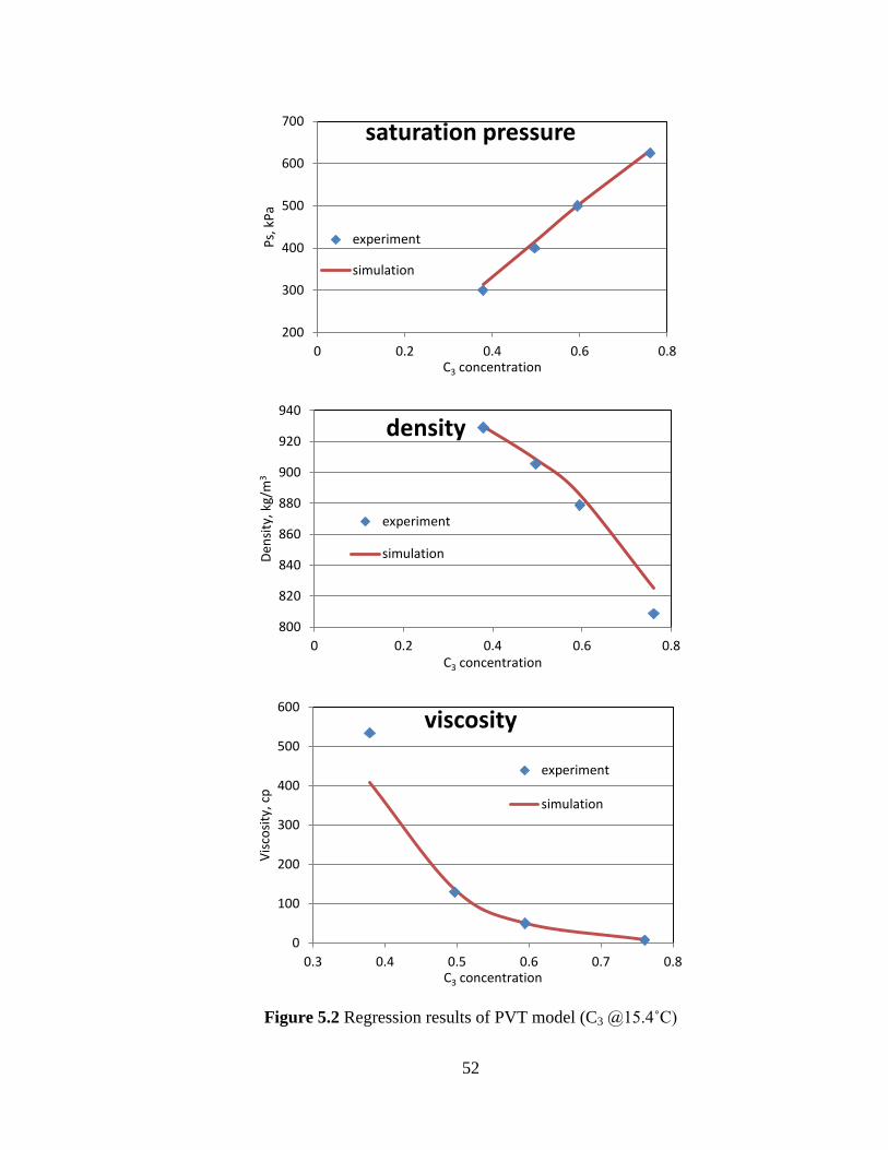
52
Figure 5.2 Regression results of PVT model (C3 @15.4˚C)
200
300
400
500
600
700
0 0.2 0.4 0.6 0.8
Ps,
kP
a
C3 concentration
saturation pressure
experiment
simulation
800
820
840
860
880
900
920
940
0 0.2 0.4 0.6 0.8
Den
sity
, kg/
m3
C3 concentration
density
experiment
simulation
0
100
200
300
400
500
600
0.3 0.4 0.5 0.6 0.7 0.8
Vis
cosi
ty, c
p
C3 concentration
viscosity
experiment
simulation
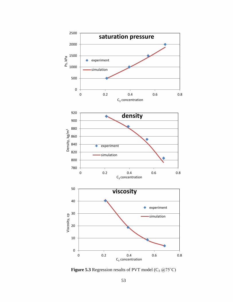
53
Figure 5.3 Regression results of PVT model (C3 @75˚C)
0
500
1000
1500
2000
2500
0 0.2 0.4 0.6 0.8
Ps,
kP
a
C3 concentration
saturation pressure
experiment
simulation
780
800
820
840
860
880
900
920
0 0.2 0.4 0.6 0.8
Den
sity
, kg/
m3
C3 concentration
density
experiment
simulation
0
10
20
30
40
50
0 0.2 0.4 0.6 0.8
Vis
cosi
ty, c
p
C3 concentration
viscosity
experiment
simulation
54
The parameters in the PVT and viscosity models of propane and the heavy oil
sample were calibrated. Figures 5.2 and 5.3 are the regression results of saturation
pressure, liquid density and liquid viscosity at two different temperatures (15.4 C and 75
C ). After the regression, the PVT and viscosity models were imported into the
simulation models.
5.3 Upscaling Study
History matching the laboratory experiments may provide valuable information. Almost
all the experimental parameters were adopted in the simulation model for the operational
constraints and the properties such as porosity, permeability, connate water saturation,
etc. In this study, the liquid-gas relative permeability curve, reaction rate, dispersion
coefficient and capillary pressure curve, which were the key factors affecting the CSI
process, were considered as the uncertain parameters.
The CSI process is very complex. In order to optimize this process, it is important
to understand the role and interactions of the various mechanisms. In this study, the
gravity override behavior and the capillary forces were believed to be the two dominant
mechanisms in the CSI process. One of the serious uncertainties for reliable field-scale
simulation is which mechanism is dominant under different reservoir conditions.
5.3.1 Sensitivity analysis
Test 4 was conducted by Model 1 with a mimic wormhole located at the bottom (see
Figure 5.4). The proportion of the wormhole length and the model length was one third.
In the injection process, the solvent (C3) was injected at 800 kPa, close to its dew point
pressure. The production well was produced at atmospheric pressure.
55
Simulations were carried out by varying only one parameter at a time to examine
its effect on the overall performance. Because the water saturation was very low in the
model, the water-oil relative permeability curve was insensitive. Therefore, the
uncertainties in upscaling the CSI process, such as the liquid-gas relative permeability
curve, the reaction rate in the foamy oil model, the dispersion coefficient and capillary
pressure were investigated by numerical simulation.
5.3.1.1 Liquid-gas relative permeability curves
One of the main fluid and formation uncertainties in the fluid flow simulation is the
relative permeability curves (Zeng 2008). Different relative permeability curves used in a
simulation model will surely yield different production performances. Figure 5.5 shows
four sets of liquid-gas relative permeability curves. The gas relative permeability curve
and liquid relative permeability curve are symmetrical in sets 1 and 4, where the only
difference is the value at both end points. One is 1, the other is 0.5. In set 2, the liquid
relative permeability curve is much lower and the value at the end point is 0.15, whereas
the end point of the gas relative permeability curve is 1. The liquid-gas relative
permeability curve of set 3 is directly opposite to that of set 2.
As shown in Figure 5.6, set 3 was the fittest relative permeability curve among the
four sets of liquid-gas relative permeability curves. In addition, during the injection of the
solvent, which is in the gas phase, the liquid-gas relative permeability curve is a key
factor to control the gas and oil. In set 3, the gas relative permeability was very small,
below 0.15, which is lower than that in typical light oil systems. Such a range of
permeability leads to very low gas mobility, which could be one of the conditions that
cause the appearance of foamy oil. Additionally, the foamy oil behavior was observed
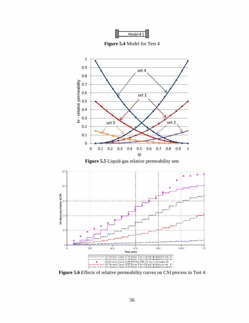
56
Figure 5.4 Model for Test 4
Figure 5.5 Liquid-gas relative permeability sets
Figure 5.6 Effects of relative permeability curves on CSI process in Test 4
0
0.1
0.2
0.3
0.4
0.5
0.6
0.7
0.8
0.9
1
0 0.1 0.2 0.3 0.4 0.5 0.6 0.7 0.8 0.9 1
kr
- re
lative p
erm
eabili
ty
Sl
set 1
set 2 set 3
set 4
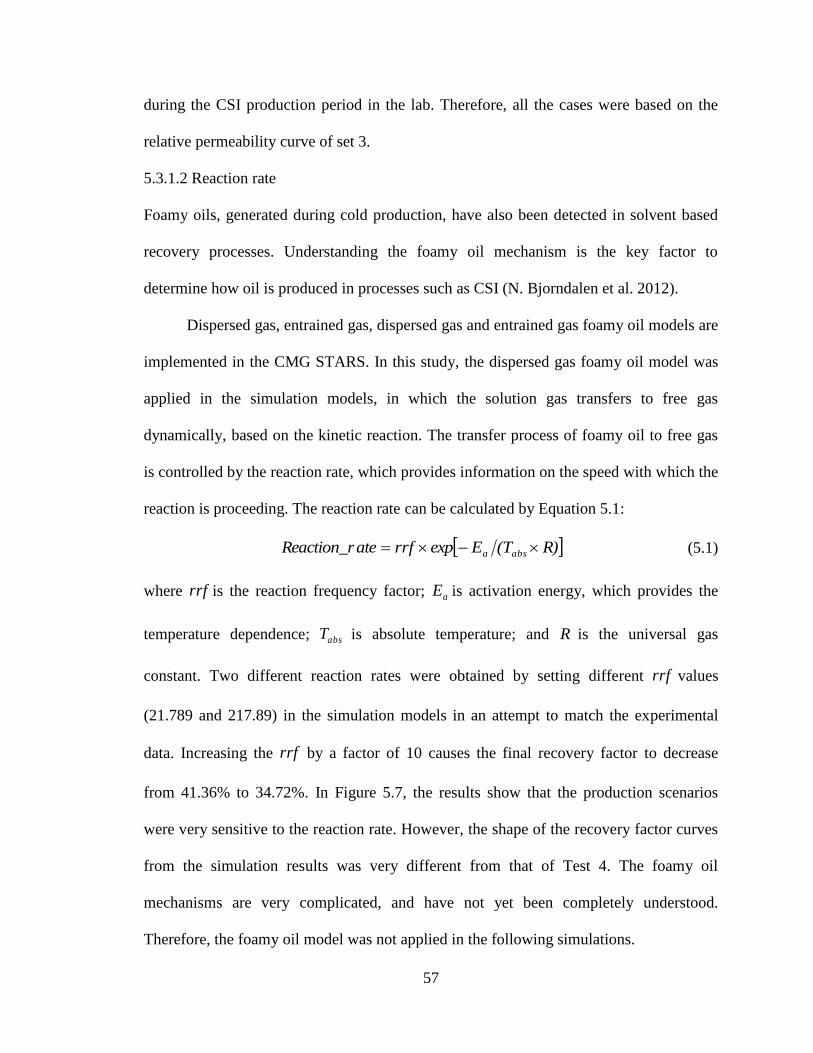
57
during the CSI production period in the lab. Therefore, all the cases were based on the
relative permeability curve of set 3.
5.3.1.2 Reaction rate
Foamy oils, generated during cold production, have also been detected in solvent based
recovery processes. Understanding the foamy oil mechanism is the key factor to
determine how oil is produced in processes such as CSI (N. Bjorndalen et al. 2012).
Dispersed gas, entrained gas, dispersed gas and entrained gas foamy oil models are
implemented in the CMG STARS. In this study, the dispersed gas foamy oil model was
applied in the simulation models, in which the solution gas transfers to free gas
dynamically, based on the kinetic reaction. The transfer process of foamy oil to free gas
is controlled by the reaction rate, which provides information on the speed with which the
reaction is proceeding. The reaction rate can be calculated by Equation 5.1:
R)(TEexprrfateReaction_r absa (5.1)
where rrf is the reaction frequency factor; aE is activation energy, which provides the
temperature dependence; absT is absolute temperature; and R is the universal gas
constant. Two different reaction rates were obtained by setting different rrf values
(21.789 and 217.89) in the simulation models in an attempt to match the experimental
data. Increasing the rrf by a factor of 10 causes the final recovery factor to decrease
from 41.36% to 34.72%. In Figure 5.7, the results show that the production scenarios
were very sensitive to the reaction rate. However, the shape of the recovery factor curves
from the simulation results was very different from that of Test 4. The foamy oil
mechanisms are very complicated, and have not yet been completely understood.
Therefore, the foamy oil model was not applied in the following simulations.
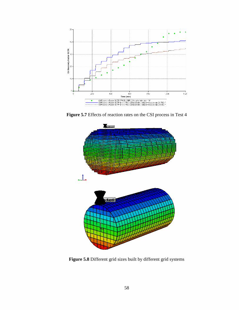
58
Figure 5.7 Effects of reaction rates on the CSI process in Test 4
Figure 5.8 Different grid sizes built by different grid systems
59
5.3.1.3 Dispersion coefficient
It is well known that finite difference simulations exhibit the effects of numerical
dispersion. In practice, the effects of numerical dispersion add to the explicit dispersion
modeled in the simulator (i.e., the dispersion assigned in the input file). The simulator is
actually modeling a larger value of dispersion than what is specified explicitly by the
user. Indeed, simulator users often include no explicit dispersion, relying on numerical
dispersion alone to model the actual dispersion in the process. Sometimes this works
fairly well (D. Cuthiell et al. 2006).
The size of the numerical dispersion effect increases with the dimensions of the
grid blocks used in the simulation. The effect of grid size was investigated in this study.
In Figure 5.8, the grid number of 313110, built with the Cartesian grid system, was
applied in Test 8, whereas the grid number of 101024, built with the orthogonal grid
system, was also applied in the same test. Figure 5.9 displays the scenarios of recovery
factors in these two cases and it shows the recovery factor is very sensitive to the grid
size. However, it is not practical and realistic, on account of the availability of facility
capacity and runtime, to refine the grid size and/or time-steps to reduce the numerical
dispersion, especially in the cyclic processes.
Figure 5.10 shows that the production scenarios were very insensitive to the
dispersion coefficient, when it was below 210-5
cm2/min. Experimental results show
that very high dispersivity results in absolute dominance of the convective dispersion,
which hardly ever occurs in either lab- or field-scale processes (Ali Yazdani and Brij B.
Maini 2009). Therefore, in this study, the dispersion coefficient was fixed as 2 10-6
cm2/min.
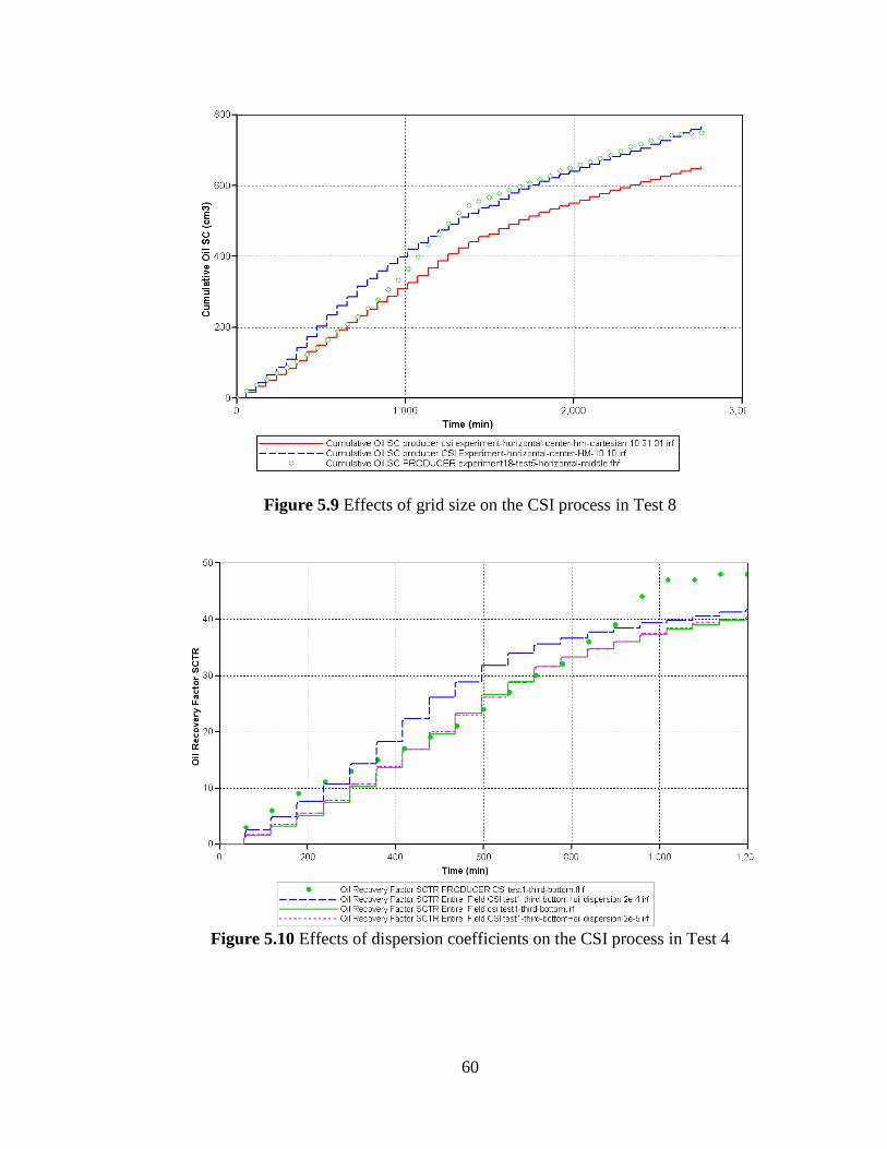
60
Figure 5.9 Effects of grid size on the CSI process in Test 8
Figure 5.10 Effects of dispersion coefficients on the CSI process in Test 4
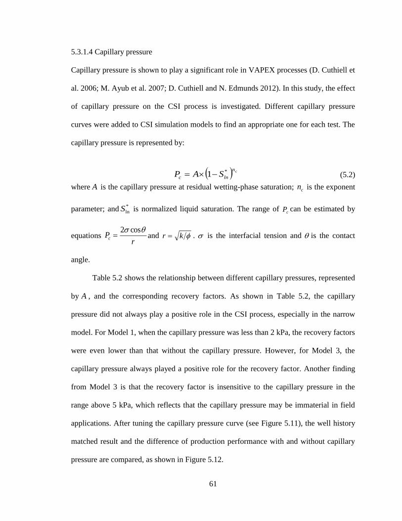
61
5.3.1.4 Capillary pressure
Capillary pressure is shown to play a significant role in VAPEX processes (D. Cuthiell et
al. 2006; M. Ayub et al. 2007; D. Cuthiell and N. Edmunds 2012). In this study, the effect
of capillary pressure on the CSI process is investigated. Different capillary pressure
curves were added to CSI simulation models to find an appropriate one for each test. The
capillary pressure is represented by:
cn*
lnc SAP 1 (5.2)
where A is the capillary pressure at residual wetting-phase saturation; cn is the exponent
parameter; and*
lnS is normalized liquid saturation. The range of cP can be estimated by
equations r
Pc
cos2 and kr . is the interfacial tension and is the contact
angle.
Table 5.2 shows the relationship between different capillary pressures, represented
by A , and the corresponding recovery factors. As shown in Table 5.2, the capillary
pressure did not always play a positive role in the CSI process, especially in the narrow
model. For Model 1, when the capillary pressure was less than 2 kPa, the recovery factors
were even lower than that without the capillary pressure. However, for Model 3, the
capillary pressure always played a positive role for the recovery factor. Another finding
from Model 3 is that the recovery factor is insensitive to the capillary pressure in the
range above 5 kPa, which reflects that the capillary pressure may be immaterial in field
applications. After tuning the capillary pressure curve (see Figure 5.11), the well history
matched result and the difference of production performance with and without capillary
pressure are compared, as shown in Figure 5.12.
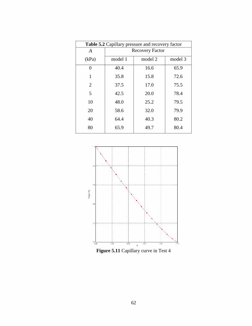
62
Table 5.2 Capillary pressure and recovery factor
A
(kPa)
Recovery Factor
model 1 model 2 model 3
0 40.4 16.6 65.9
1 35.8 15.8 72.6
2 37.5 17.0 75.5
5 42.5 20.0 78.4
10 48.0 25.2 79.5
20 58.6 32.0 79.9
40 64.4 40.3 80.2
80 65.9 49.7 80.4
Figure 5.11 Capillary curve in Test 4
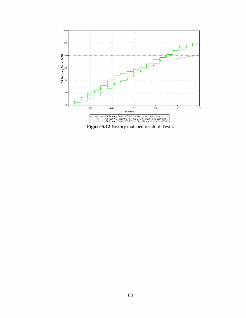
63
Figure 5.12 History matched result of Test 4
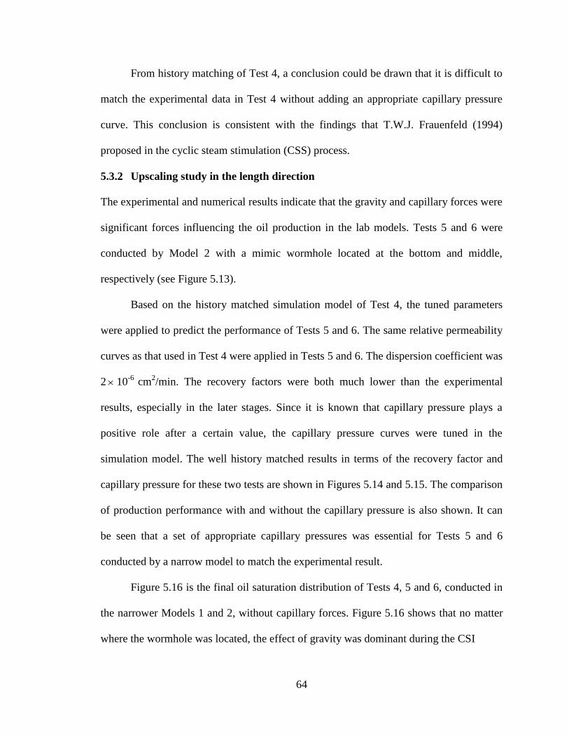
64
From history matching of Test 4, a conclusion could be drawn that it is difficult to
match the experimental data in Test 4 without adding an appropriate capillary pressure
curve. This conclusion is consistent with the findings that T.W.J. Frauenfeld (1994)
proposed in the cyclic steam stimulation (CSS) process.
5.3.2 Upscaling study in the length direction
The experimental and numerical results indicate that the gravity and capillary forces were
significant forces influencing the oil production in the lab models. Tests 5 and 6 were
conducted by Model 2 with a mimic wormhole located at the bottom and middle,
respectively (see Figure 5.13).
Based on the history matched simulation model of Test 4, the tuned parameters
were applied to predict the performance of Tests 5 and 6. The same relative permeability
curves as that used in Test 4 were applied in Tests 5 and 6. The dispersion coefficient was
2 10-6
cm2/min. The recovery factors were both much lower than the experimental
results, especially in the later stages. Since it is known that capillary pressure plays a
positive role after a certain value, the capillary pressure curves were tuned in the
simulation model. The well history matched results in terms of the recovery factor and
capillary pressure for these two tests are shown in Figures 5.14 and 5.15. The comparison
of production performance with and without the capillary pressure is also shown. It can
be seen that a set of appropriate capillary pressures was essential for Tests 5 and 6
conducted by a narrow model to match the experimental result.
Figure 5.16 is the final oil saturation distribution of Tests 4, 5 and 6, conducted in
the narrower Models 1 and 2, without capillary forces. Figure 5.16 shows that no matter
where the wormhole was located, the effect of gravity was dominant during the CSI
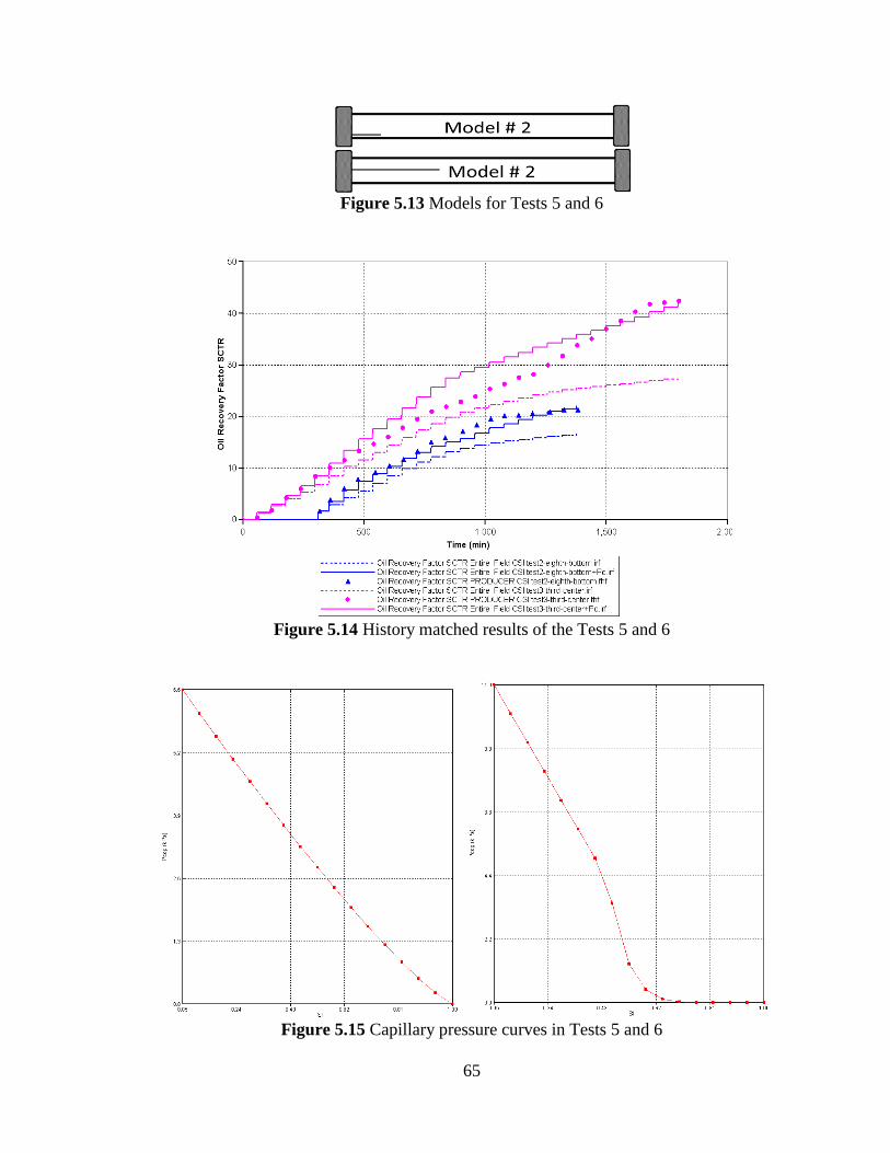
65
Figure 5.13 Models for Tests 5 and 6
Figure 5.14 History matched results of the Tests 5 and 6
Figure 5.15 Capillary pressure curves in Tests 5 and 6
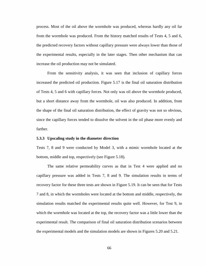
66
process. Most of the oil above the wormhole was produced, whereas hardly any oil far
from the wormhole was produced. From the history matched results of Tests 4, 5 and 6,
the predicted recovery factors without capillary pressure were always lower than those of
the experimental results, especially in the later stages. Then other mechanism that can
increase the oil production may not be simulated.
From the sensitivity analysis, it was seen that inclusion of capillary forces
increased the predicted oil production. Figure 5.17 is the final oil saturation distribution
of Tests 4, 5 and 6 with capillary forces. Not only was oil above the wormhole produced,
but a short distance away from the wormhole, oil was also produced. In addition, from
the shape of the final oil saturation distribution, the effect of gravity was not so obvious,
since the capillary forces tended to dissolve the solvent in the oil phase more evenly and
farther.
5.3.3 Upscaling study in the diameter direction
Tests 7, 8 and 9 were conducted by Model 3, with a mimic wormhole located at the
bottom, middle and top, respectively (see Figure 5.18).
The same relative permeability curves as that in Test 4 were applied and no
capillary pressure was added in Tests 7, 8 and 9. The simulation results in terms of
recovery factor for these three tests are shown in Figure 5.19. It can be seen that for Tests
7 and 8, in which the wormholes were located at the bottom and middle, respectively, the
simulation results matched the experimental results quite well. However, for Test 9, in
which the wormhole was located at the top, the recovery factor was a little lower than the
experimental result. The comparison of final oil saturation distribution scenarios between
the experimental models and the simulation models are shown in Figures 5.20 and 5.21.
67
Figure 5.16 Final oil saturation distribution of Tests 4, 5 and 6 without cP
Figure 5.17 Final oil saturation distribution of Tests 4, 5 and 6 with cP
Figure 5.18 Wormhole locations in Tests 7, 8 and 9
Figure 5.19 History matched results of Tests 7, 8 and 9
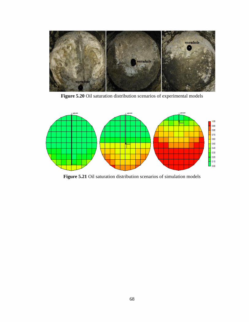
68
Figure 5.20 Oil saturation distribution scenarios of experimental models
Figure 5.21 Oil saturation distribution scenarios of simulation models
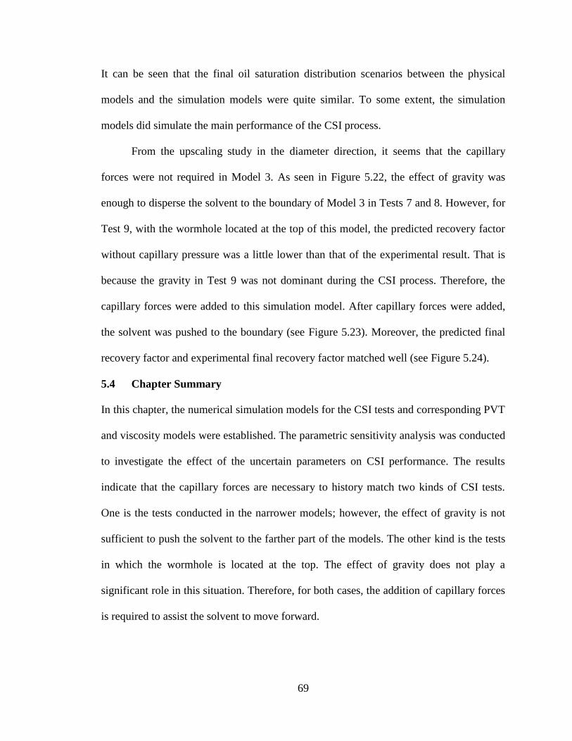
69
It can be seen that the final oil saturation distribution scenarios between the physical
models and the simulation models were quite similar. To some extent, the simulation
models did simulate the main performance of the CSI process.
From the upscaling study in the diameter direction, it seems that the capillary
forces were not required in Model 3. As seen in Figure 5.22, the effect of gravity was
enough to disperse the solvent to the boundary of Model 3 in Tests 7 and 8. However, for
Test 9, with the wormhole located at the top of this model, the predicted recovery factor
without capillary pressure was a little lower than that of the experimental result. That is
because the gravity in Test 9 was not dominant during the CSI process. Therefore, the
capillary forces were added to this simulation model. After capillary forces were added,
the solvent was pushed to the boundary (see Figure 5.23). Moreover, the predicted final
recovery factor and experimental final recovery factor matched well (see Figure 5.24).
5.4 Chapter Summary
In this chapter, the numerical simulation models for the CSI tests and corresponding PVT
and viscosity models were established. The parametric sensitivity analysis was conducted
to investigate the effect of the uncertain parameters on CSI performance. The results
indicate that the capillary forces are necessary to history match two kinds of CSI tests.
One is the tests conducted in the narrower models; however, the effect of gravity is not
sufficient to push the solvent to the farther part of the models. The other kind is the tests
in which the wormhole is located at the top. The effect of gravity does not play a
significant role in this situation. Therefore, for both cases, the addition of capillary forces
is required to assist the solvent to move forward.
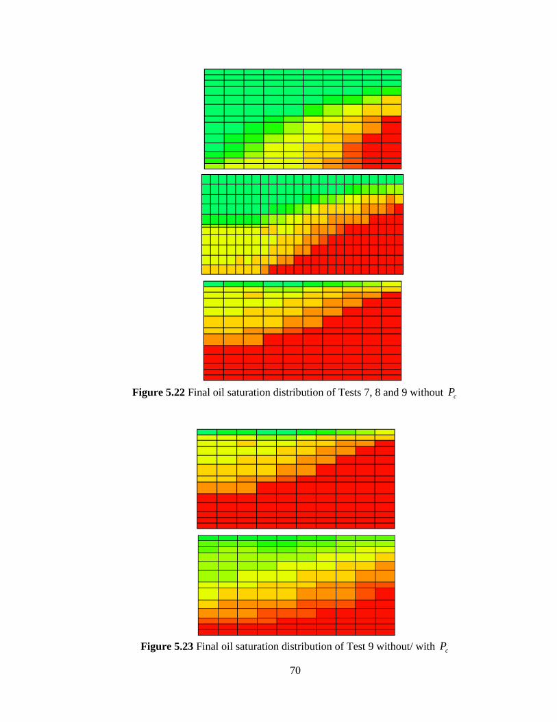
70
Figure 5.22 Final oil saturation distribution of Tests 7, 8 and 9 without cP
Figure 5.23 Final oil saturation distribution of Test 9 without/ with cP
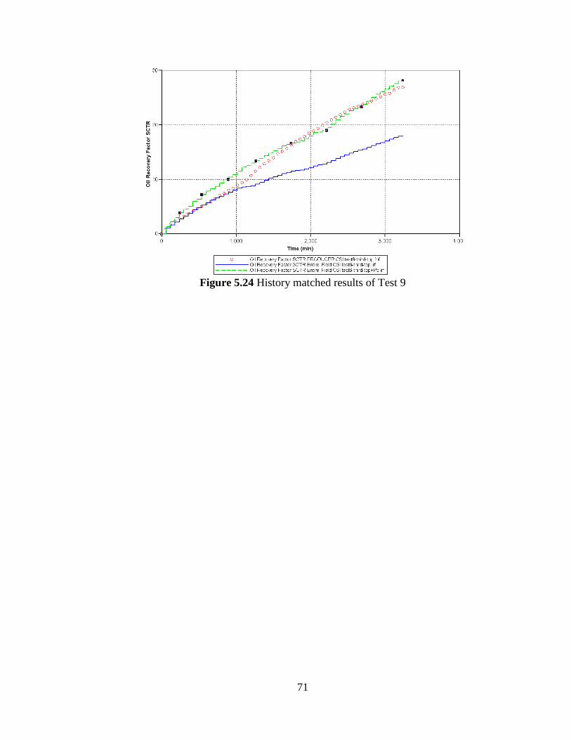
71
Figure 5.24 History matched results of Test 9
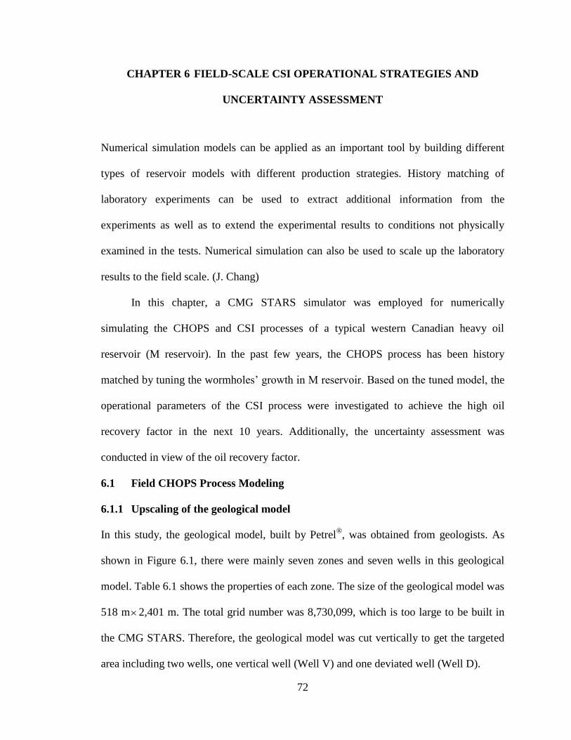
72
CHAPTER 6 FIELD-SCALE CSI OPERATIONAL STRATEGIES AND
UNCERTAINTY ASSESSMENT
Numerical simulation models can be applied as an important tool by building different
types of reservoir models with different production strategies. History matching of
laboratory experiments can be used to extract additional information from the
experiments as well as to extend the experimental results to conditions not physically
examined in the tests. Numerical simulation can also be used to scale up the laboratory
results to the field scale. (J. Chang)
In this chapter, a CMG STARS simulator was employed for numerically
simulating the CHOPS and CSI processes of a typical western Canadian heavy oil
reservoir (M reservoir). In the past few years, the CHOPS process has been history
matched by tuning the wormholes’ growth in M reservoir. Based on the tuned model, the
operational parameters of the CSI process were investigated to achieve the high oil
recovery factor in the next 10 years. Additionally, the uncertainty assessment was
conducted in view of the oil recovery factor.
6.1 Field CHOPS Process Modeling
6.1.1 Upscaling of the geological model
In this study, the geological model, built by Petrel®, was obtained from geologists. As
shown in Figure 6.1, there were mainly seven zones and seven wells in this geological
model. Table 6.1 shows the properties of each zone. The size of the geological model was
518 m2,401 m. The total grid number was 8,730,099, which is too large to be built in
the CMG STARS. Therefore, the geological model was cut vertically to get the targeted
area including two wells, one vertical well (Well V) and one deviated well (Well D).
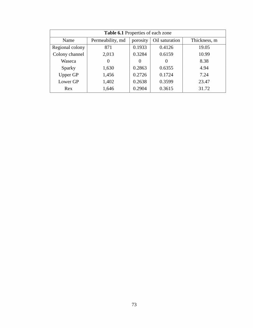
73
Table 6.1 Properties of each zone
Name Permeability, md porosity Oil saturation Thickness, m
Regional colony 871 0.1933 0.4126 19.05
Colony channel 2,013 0.3284 0.6159 10.99
Waseca 0 0 0 8.38
Sparky 1,630 0.2863 0.6355 4.94
Upper GP 1,456 0.2726 0.1724 7.24
Lower GP 1,402 0.2638 0.3599 23.47
Rex 1,646 0.2904 0.3615 31.72
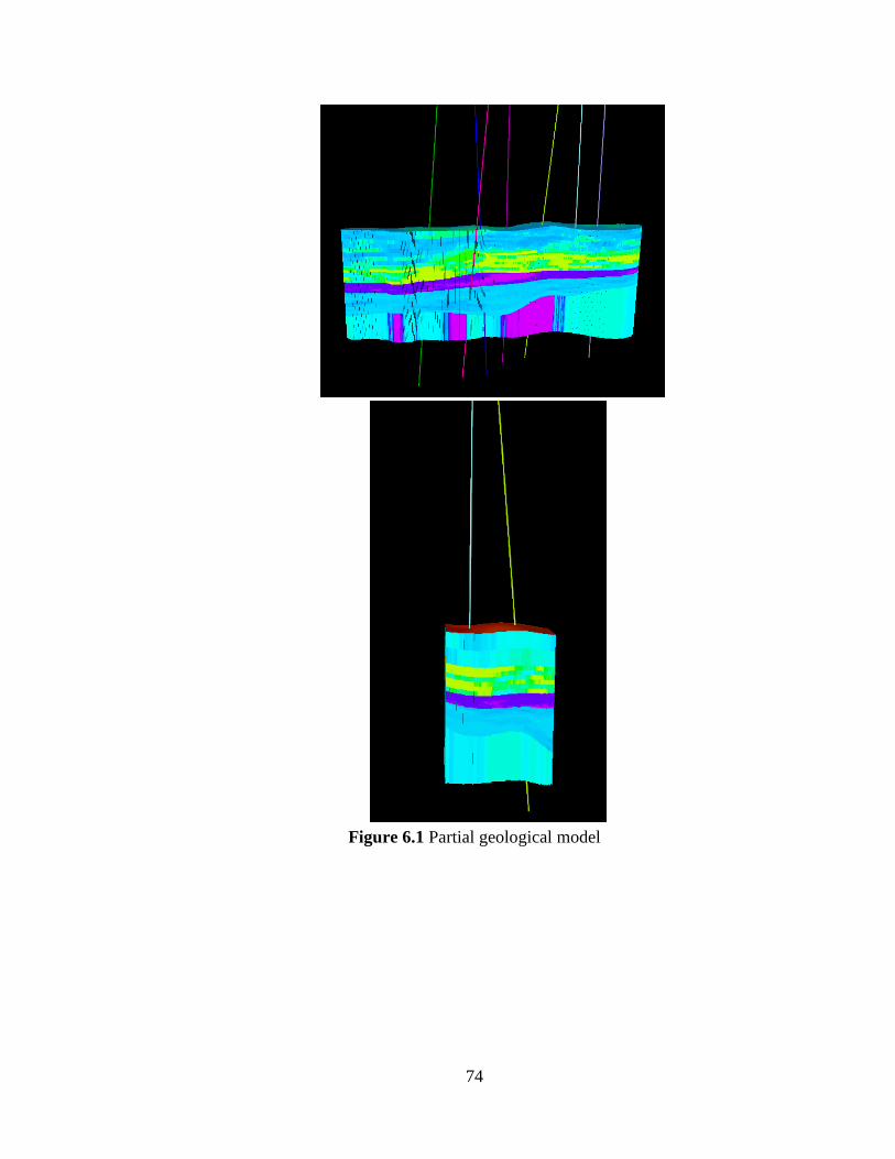
74
Figure 6.1 Partial geological model
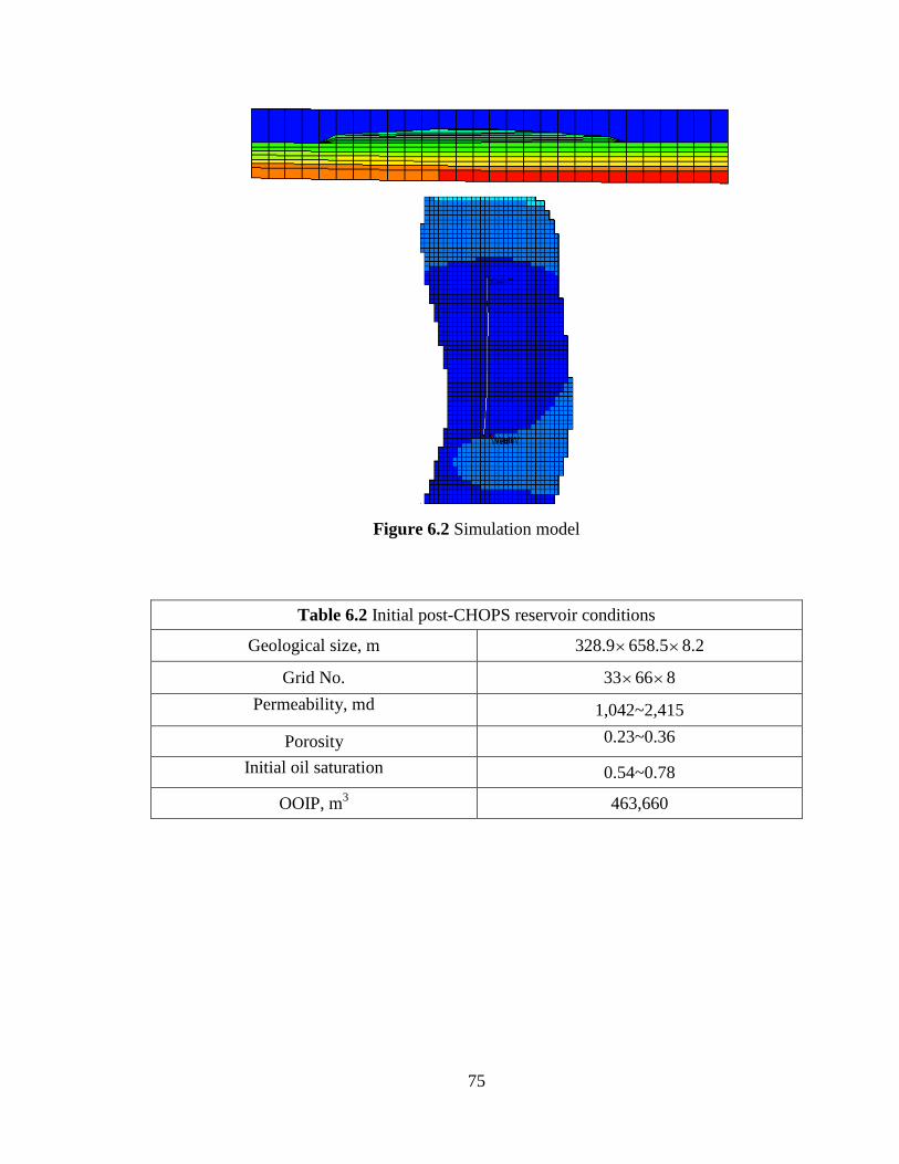
75
Figure 6.2 Simulation model
Table 6.2 Initial post-CHOPS reservoir conditions
Geological size, m 328.9658.58.2
Grid No. 33668
Permeability, md
1,042~2,415
Porosity 0.23~0.36
Initial oil saturation
0.54~0.78
OOIP, m3 463,660
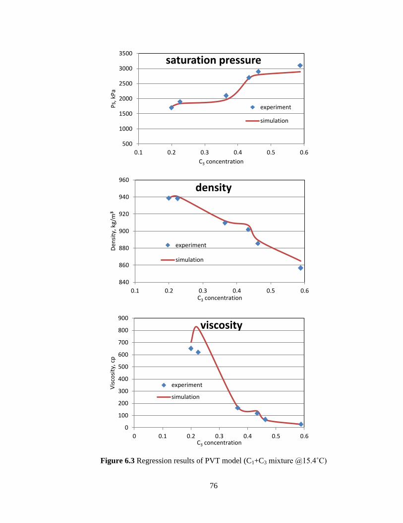
76
Figure 6.3 Regression results of PVT model (C1+C3 mixture @15.4˚C)
500
1000
1500
2000
2500
3000
3500
0.1 0.2 0.3 0.4 0.5 0.6
Ps,
kP
a
C3 concentration
saturation pressure
experiment
simulation
840
860
880
900
920
940
960
0.1 0.2 0.3 0.4 0.5 0.6
Den
sity
, kg/
m3
C3 concentration
density
experiment
simulation
0
100
200
300
400
500
600
700
800
900
0 0.1 0.2 0.3 0.4 0.5 0.6
Vis
cosi
ty, c
p
C3 concentration
viscosity
experiment
simulation
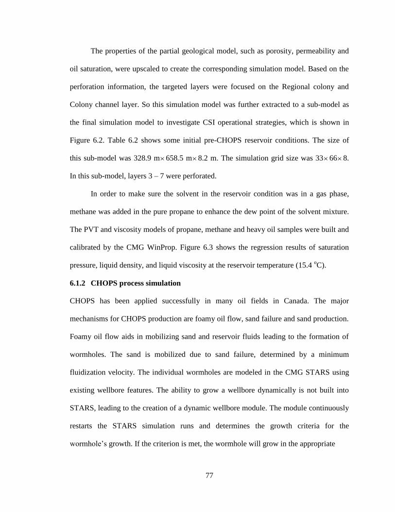
77
The properties of the partial geological model, such as porosity, permeability and
oil saturation, were upscaled to create the corresponding simulation model. Based on the
perforation information, the targeted layers were focused on the Regional colony and
Colony channel layer. So this simulation model was further extracted to a sub-model as
the final simulation model to investigate CSI operational strategies, which is shown in
Figure 6.2. Table 6.2 shows some initial pre-CHOPS reservoir conditions. The size of
this sub-model was 328.9 m658.5 m8.2 m. The simulation grid size was 33668.
In this sub-model, layers 3 – 7 were perforated.
In order to make sure the solvent in the reservoir condition was in a gas phase,
methane was added in the pure propane to enhance the dew point of the solvent mixture.
The PVT and viscosity models of propane, methane and heavy oil samples were built and
calibrated by the CMG WinProp. Figure 6.3 shows the regression results of saturation
pressure, liquid density, and liquid viscosity at the reservoir temperature (15.4 oC).
6.1.2 CHOPS process simulation
CHOPS has been applied successfully in many oil fields in Canada. The major
mechanisms for CHOPS production are foamy oil flow, sand failure and sand production.
Foamy oil flow aids in mobilizing sand and reservoir fluids leading to the formation of
wormholes. The sand is mobilized due to sand failure, determined by a minimum
fluidization velocity. The individual wormholes are modeled in the CMG STARS using
existing wellbore features. The ability to grow a wellbore dynamically is not built into
STARS, leading to the creation of a dynamic wellbore module. The module continuously
restarts the STARS simulation runs and determines the growth criteria for the
wormhole’s growth. If the criterion is met, the wormhole will grow in the appropriate
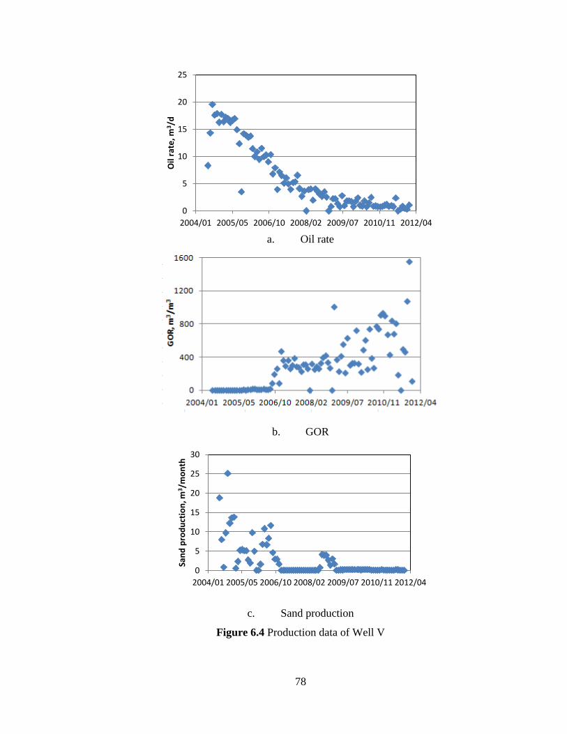
78
a. Oil rate
b. GOR
c. Sand production
Figure 6.4 Production data of Well V
0
5
10
15
20
25
2004/01 2005/05 2006/10 2008/02 2009/07 2010/11 2012/04
Oil
rate
, m3/d
0
5
10
15
20
25
30
2004/01 2005/05 2006/10 2008/02 2009/07 2010/11 2012/04
San
d p
rod
uct
ion
, m3 /
mo
nth
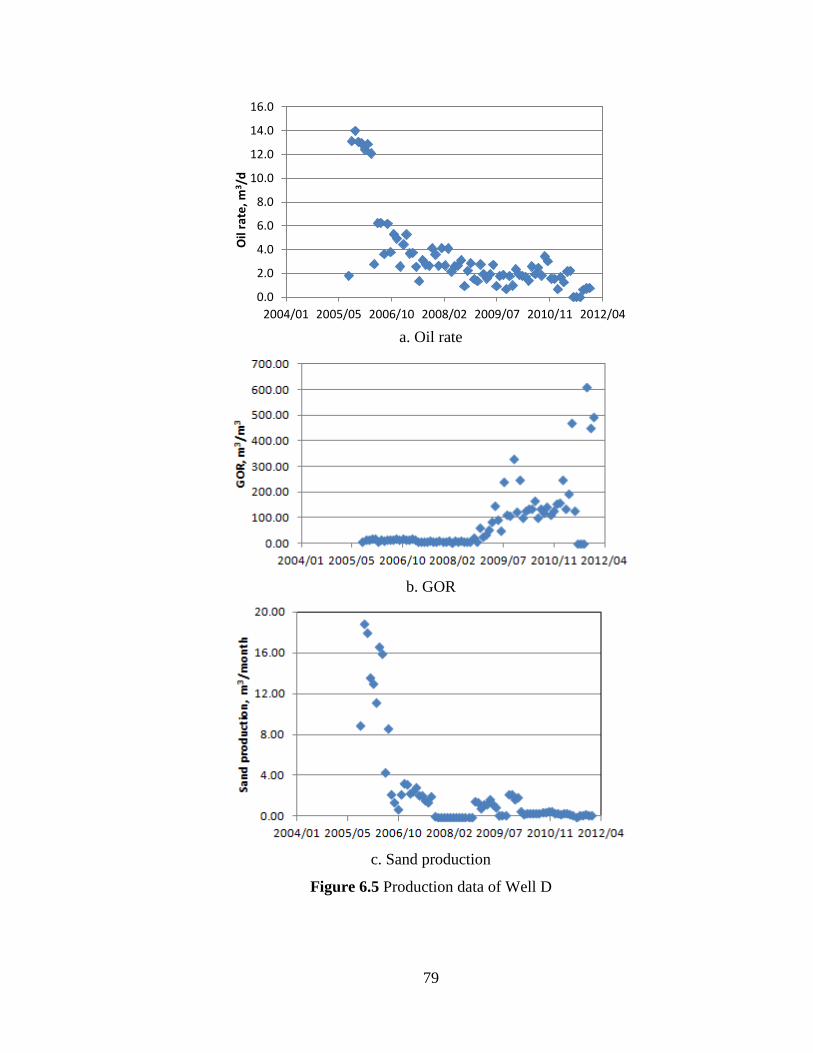
79
a. Oil rate
b. GOR
c. Sand production
Figure 6.5 Production data of Well D
0.0
2.0
4.0
6.0
8.0
10.0
12.0
14.0
16.0
2004/01 2005/05 2006/10 2008/02 2009/07 2010/11 2012/04
Oil
rate
, m3 /
d
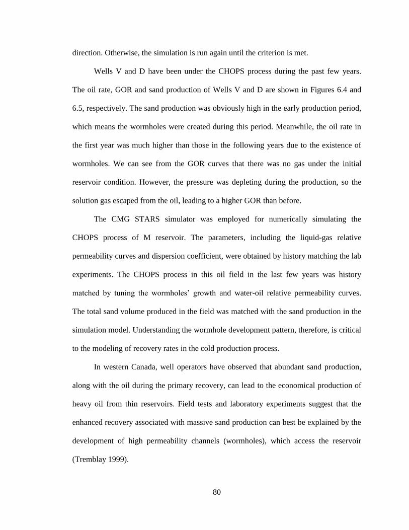
80
direction. Otherwise, the simulation is run again until the criterion is met.
Wells V and D have been under the CHOPS process during the past few years.
The oil rate, GOR and sand production of Wells V and D are shown in Figures 6.4 and
6.5, respectively. The sand production was obviously high in the early production period,
which means the wormholes were created during this period. Meanwhile, the oil rate in
the first year was much higher than those in the following years due to the existence of
wormholes. We can see from the GOR curves that there was no gas under the initial
reservoir condition. However, the pressure was depleting during the production, so the
solution gas escaped from the oil, leading to a higher GOR than before.
The CMG STARS simulator was employed for numerically simulating the
CHOPS process of M reservoir. The parameters, including the liquid-gas relative
permeability curves and dispersion coefficient, were obtained by history matching the lab
experiments. The CHOPS process in this oil field in the last few years was history
matched by tuning the wormholes’ growth and water-oil relative permeability curves.
The total sand volume produced in the field was matched with the sand production in the
simulation model. Understanding the wormhole development pattern, therefore, is critical
to the modeling of recovery rates in the cold production process.
In western Canada, well operators have observed that abundant sand production,
along with the oil during the primary recovery, can lead to the economical production of
heavy oil from thin reservoirs. Field tests and laboratory experiments suggest that the
enhanced recovery associated with massive sand production can best be explained by the
development of high permeability channels (wormholes), which access the reservoir
(Tremblay 1999).
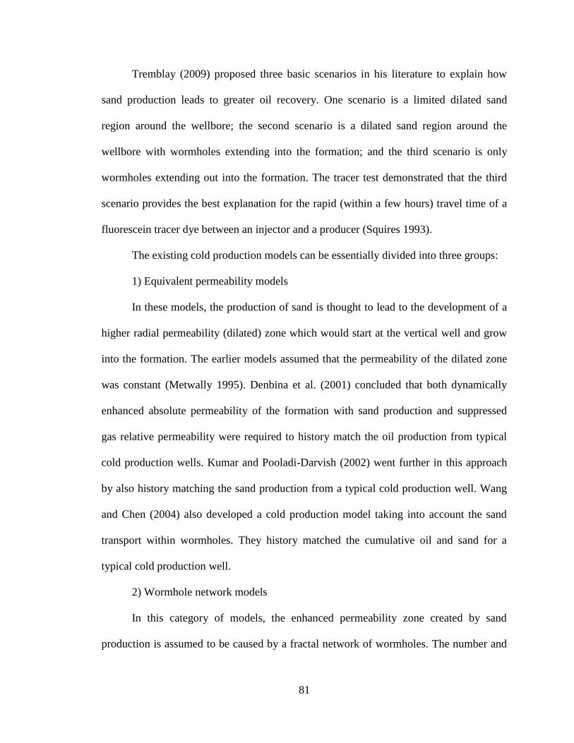
81
Tremblay (2009) proposed three basic scenarios in his literature to explain how
sand production leads to greater oil recovery. One scenario is a limited dilated sand
region around the wellbore; the second scenario is a dilated sand region around the
wellbore with wormholes extending into the formation; and the third scenario is only
wormholes extending out into the formation. The tracer test demonstrated that the third
scenario provides the best explanation for the rapid (within a few hours) travel time of a
fluorescein tracer dye between an injector and a producer (Squires 1993).
The existing cold production models can be essentially divided into three groups:
1) Equivalent permeability models
In these models, the production of sand is thought to lead to the development of a
higher radial permeability (dilated) zone which would start at the vertical well and grow
into the formation. The earlier models assumed that the permeability of the dilated zone
was constant (Metwally 1995). Denbina et al. (2001) concluded that both dynamically
enhanced absolute permeability of the formation with sand production and suppressed
gas relative permeability were required to history match the oil production from typical
cold production wells. Kumar and Pooladi-Darvish (2002) went further in this approach
by also history matching the sand production from a typical cold production well. Wang
and Chen (2004) also developed a cold production model taking into account the sand
transport within wormholes. They history matched the cumulative oil and sand for a
typical cold production well.
2) Wormhole network models
In this category of models, the enhanced permeability zone created by sand
production is assumed to be caused by a fractal network of wormholes. The number and
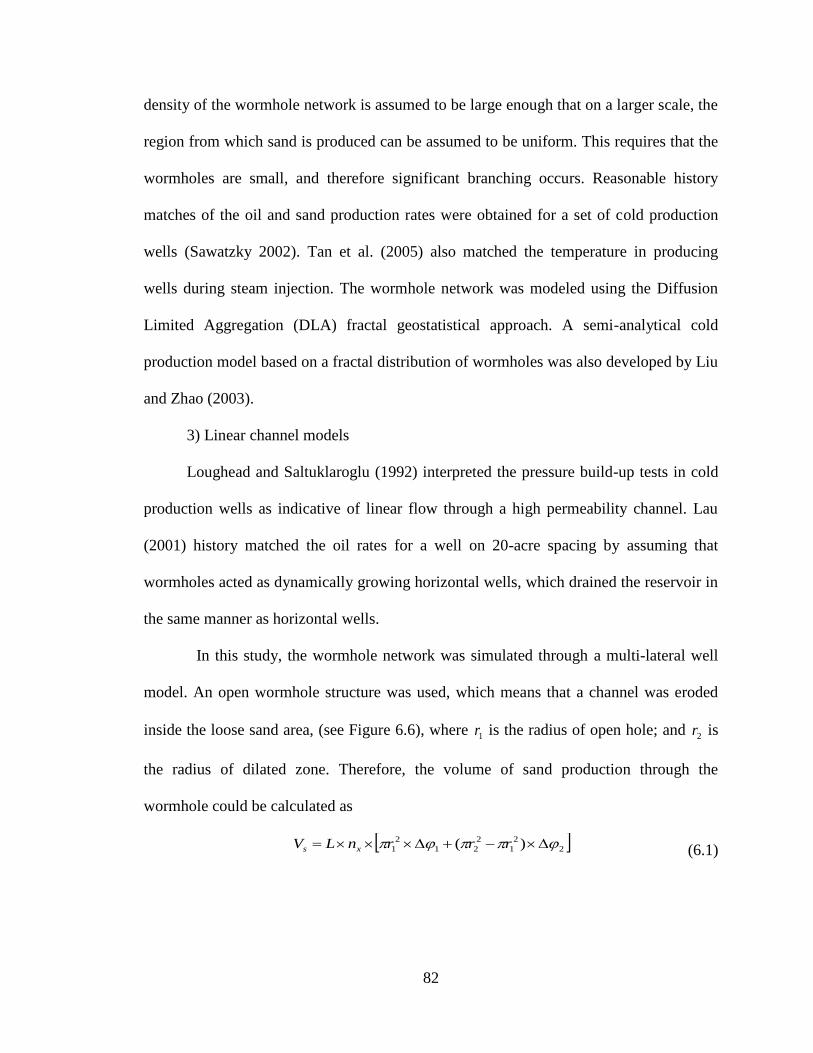
82
density of the wormhole network is assumed to be large enough that on a larger scale, the
region from which sand is produced can be assumed to be uniform. This requires that the
wormholes are small, and therefore significant branching occurs. Reasonable history
matches of the oil and sand production rates were obtained for a set of cold production
wells (Sawatzky 2002). Tan et al. (2005) also matched the temperature in producing
wells during steam injection. The wormhole network was modeled using the Diffusion
Limited Aggregation (DLA) fractal geostatistical approach. A semi-analytical cold
production model based on a fractal distribution of wormholes was also developed by Liu
and Zhao (2003).
3) Linear channel models
Loughead and Saltuklaroglu (1992) interpreted the pressure build-up tests in cold
production wells as indicative of linear flow through a high permeability channel. Lau
(2001) history matched the oil rates for a well on 20-acre spacing by assuming that
wormholes acted as dynamically growing horizontal wells, which drained the reservoir in
the same manner as horizontal wells.
In this study, the wormhole network was simulated through a multi-lateral well
model. An open wormhole structure was used, which means that a channel was eroded
inside the loose sand area, (see Figure 6.6), where 1r is the radius of open hole; and 2r is
the radius of dilated zone. Therefore, the volume of sand production through the
wormhole could be calculated as
2
2
1
2
21
2
1 )( rrrnLV xs (6.1)
83
Figure 6.6 Wormhole structure
Figure 6.7 Wormhole structure in the 5th layer
r2
r1
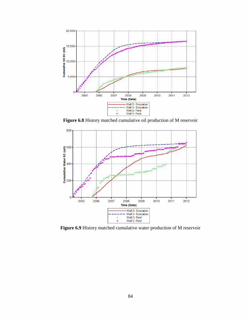
84
Figure 6.8 History matched cumulative oil production of M reservoir
Figure 6.9 History matched cumulative water production of M reservoir
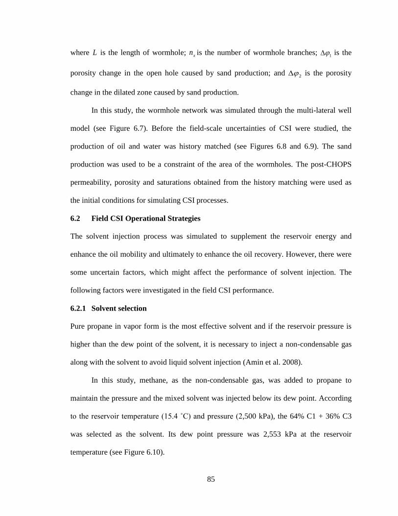
85
where L is the length of wormhole; xn is the number of wormhole branches; 1 is the
porosity change in the open hole caused by sand production; and 2 is the porosity
change in the dilated zone caused by sand production.
In this study, the wormhole network was simulated through the multi-lateral well
model (see Figure 6.7). Before the field-scale uncertainties of CSI were studied, the
production of oil and water was history matched (see Figures 6.8 and 6.9). The sand
production was used to be a constraint of the area of the wormholes. The post-CHOPS
permeability, porosity and saturations obtained from the history matching were used as
the initial conditions for simulating CSI processes.
6.2 Field CSI Operational Strategies
The solvent injection process was simulated to supplement the reservoir energy and
enhance the oil mobility and ultimately to enhance the oil recovery. However, there were
some uncertain factors, which might affect the performance of solvent injection. The
following factors were investigated in the field CSI performance.
6.2.1 Solvent selection
Pure propane in vapor form is the most effective solvent and if the reservoir pressure is
higher than the dew point of the solvent, it is necessary to inject a non-condensable gas
along with the solvent to avoid liquid solvent injection (Amin et al. 2008).
In this study, methane, as the non-condensable gas, was added to propane to
maintain the pressure and the mixed solvent was injected below its dew point. According
to the reservoir temperature (15.4 ˚C) and pressure (2,500 kPa), the 64% C1 + 36% C3
was selected as the solvent. Its dew point pressure was 2,553 kPa at the reservoir
temperature (see Figure 6.10).
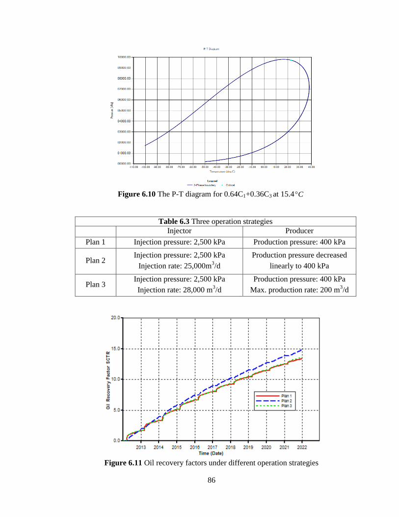
86
Figure 6.10 The P-T diagram for 0.64C1+0.36C3 at 15.4 C
Table 6.3 Three operation strategies
Injector Producer
Plan 1 Injection pressure: 2,500 kPa Production pressure: 400 kPa
Plan 2 Injection pressure: 2,500 kPa
Injection rate: 25,000m3/d
Production pressure decreased
linearly to 400 kPa
Plan 3 Injection pressure: 2,500 kPa
Injection rate: 28,000 m3/d
Production pressure: 400 kPa
Max. production rate: 200 m3/d
Figure 6.11 Oil recovery factors under different operation strategies
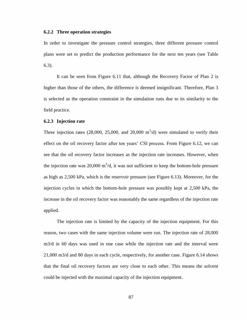
87
6.2.2 Three operation strategies
In order to investigate the pressure control strategies, three different pressure control
plans were set to predict the production performance for the next ten years (see Table
6.3).
It can be seen from Figure 6.11 that, although the Recovery Factor of Plan 2 is
higher than those of the others, the difference is deemed insignificant. Therefore, Plan 3
is selected as the operation constraint in the simulation runs due to its similarity to the
field practice.
6.2.3 Injection rate
Three injection rates (28,000, 25,000, and 20,000 m3/d) were simulated to verify their
effect on the oil recovery factor after ten years’ CSI process. From Figure 6.12, we can
see that the oil recovery factor increases as the injection rate increases. However, when
the injection rate was 20,000 m3/d, it was not sufficient to keep the bottom-hole pressure
as high as 2,500 kPa, which is the reservoir pressure (see Figure 6.13). Moreover, for the
injection cycles in which the bottom-hole pressure was possibly kept at 2,500 kPa, the
increase in the oil recovery factor was reasonably the same regardless of the injection rate
applied.
The injection rate is limited by the capacity of the injection equipment. For this
reason, two cases with the same injection volume were run. The injection rate of 28,000
m3/d in 60 days was used in one case while the injection rate and the interval were
21,000 m3/d and 80 days in each cycle, respectively, for another case. Figure 6.14 shows
that the final oil recovery factors are very close to each other. This means the solvent
could be injected with the maximal capacity of the injection equipment.
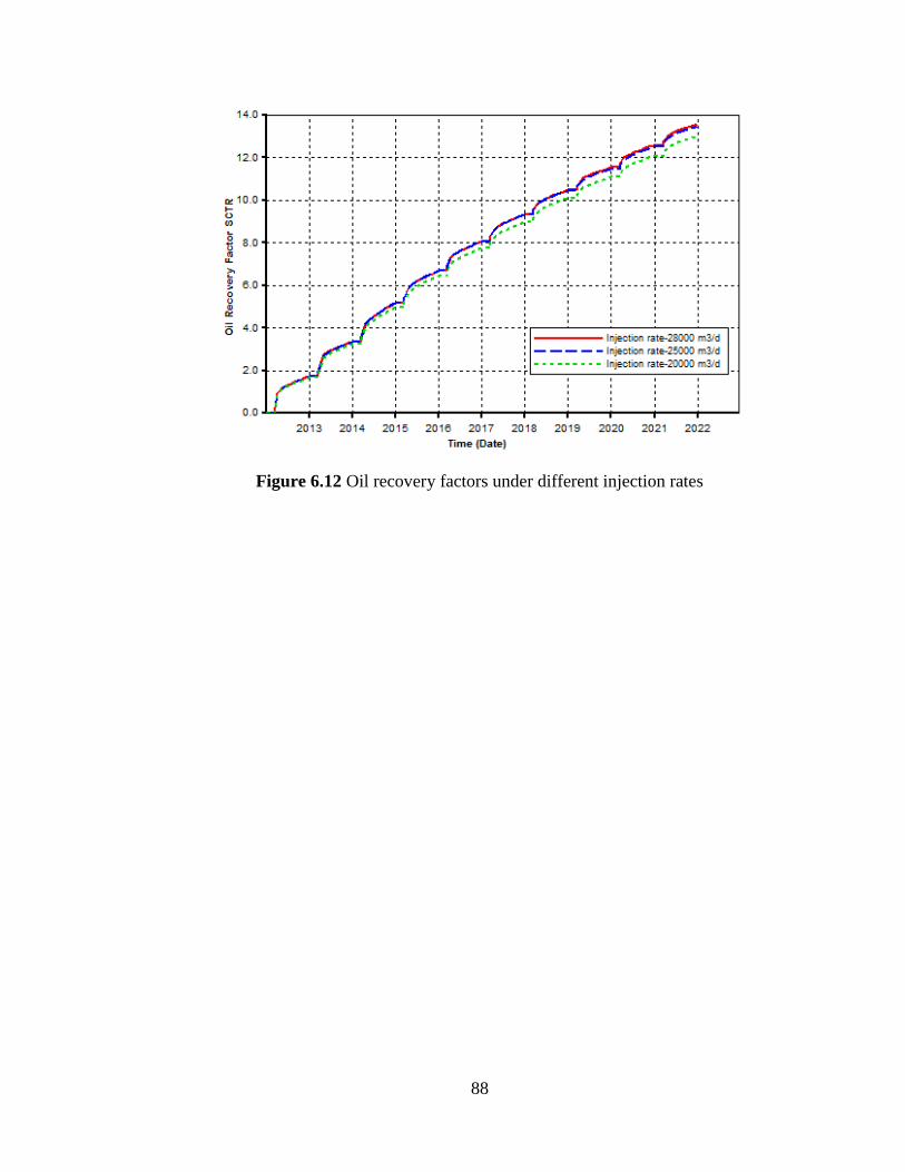
88
Figure 6.12 Oil recovery factors under different injection rates
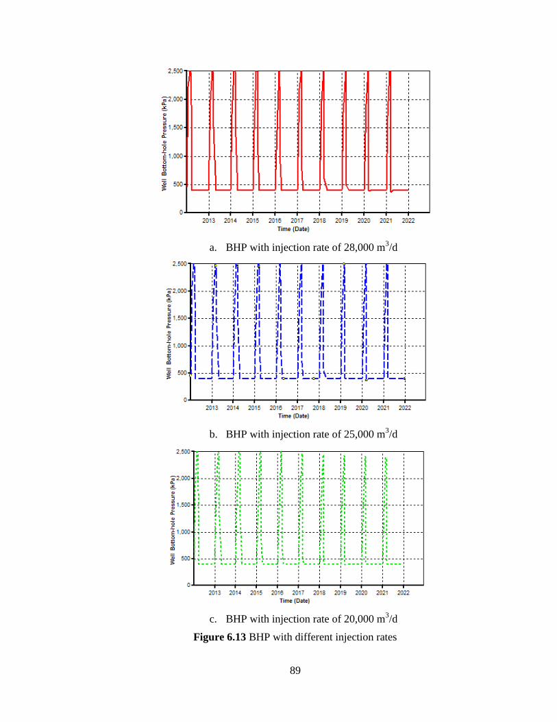
89
a. BHP with injection rate of 28,000 m3/d
b. BHP with injection rate of 25,000 m3/d
c. BHP with injection rate of 20,000 m3/d
Figure 6.13 BHP with different injection rates
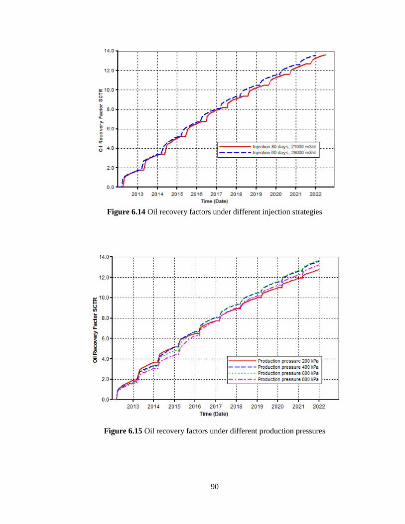
90
Figure 6.14 Oil recovery factors under different injection strategies
Figure 6.15 Oil recovery factors under different production pressures
91
6.2.4 Production pressure
Four production pressures (200 kPa, 400 kPa, 600 kPa and 800 kPa) were investigated in
this project. From Figure 6.15, we can see that the oil recovery factor is the highest when
the production pressure is the lowest (200 kPa) in the first three cycles. However, the
lowest production pressure gives the lowest recovery factor in the end. The highest
recovery factor is achieved when the bottom-hole pressure is set at 600 kPa.
6.2.5 Production rate
Different maximum production rates (400 m3/d, 200 m
3/d, 50 m
3/d and 25 m
3/d) were set
as the production well constraint. The oil recovery factor increases with the reduction in
the maximum production rate (see Figure 6.16).
6.2.6 Soaking time
The length of soaking time (15 days, 30 days and 45 days) was also investigated in this
study. Figure 6.17 shows that the oil recovery factors are essentially the same for the
different soaking periods, indicating that soaking time is an insensitive parameter. As a
result, the soaking time is not necessarily required to be long, and a higher economic
feasibility can be accomplished by minimizing the soaking period.
6.2.7 Injection pressure
Table 6.4 shows three cases with different injection pressures. Different compositions of
solvent mixture were applied in order to keep the injection pressure below its dew point.
Both injection and production were controlled by pressure. Figure 6.18 shows P-T
diagrams of solvent mixture at the reservoir temperature.
Figure 6.19 shows that the oil recovery factor increases with increasing injection
pressure at the expense of the increase in cumulative injection gas volume (see Figure
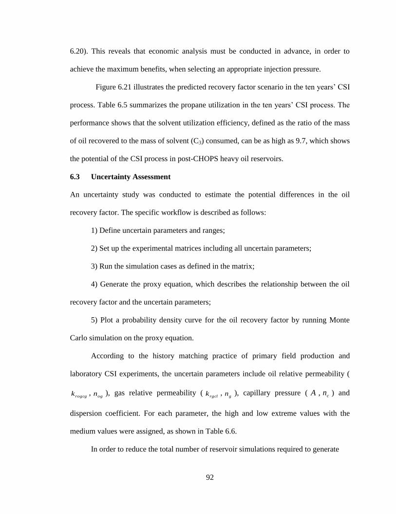
92
6.20). This reveals that economic analysis must be conducted in advance, in order to
achieve the maximum benefits, when selecting an appropriate injection pressure.
Figure 6.21 illustrates the predicted recovery factor scenario in the ten years’ CSI
process. Table 6.5 summarizes the propane utilization in the ten years’ CSI process. The
performance shows that the solvent utilization efficiency, defined as the ratio of the mass
of oil recovered to the mass of solvent (C3) consumed, can be as high as 9.7, which shows
the potential of the CSI process in post-CHOPS heavy oil reservoirs.
6.3 Uncertainty Assessment
An uncertainty study was conducted to estimate the potential differences in the oil
recovery factor. The specific workflow is described as follows:
1) Define uncertain parameters and ranges;
2) Set up the experimental matrices including all uncertain parameters;
3) Run the simulation cases as defined in the matrix;
4) Generate the proxy equation, which describes the relationship between the oil
recovery factor and the uncertain parameters;
5) Plot a probability density curve for the oil recovery factor by running Monte
Carlo simulation on the proxy equation.
According to the history matching practice of primary field production and
laboratory CSI experiments, the uncertain parameters include oil relative permeability (
rogcgk ,ogn ), gas relative permeability (
rgclk ,gn ), capillary pressure ( A , cn ) and
dispersion coefficient. For each parameter, the high and low extreme values with the
medium values were assigned, as shown in Table 6.6.
In order to reduce the total number of reservoir simulations required to generate
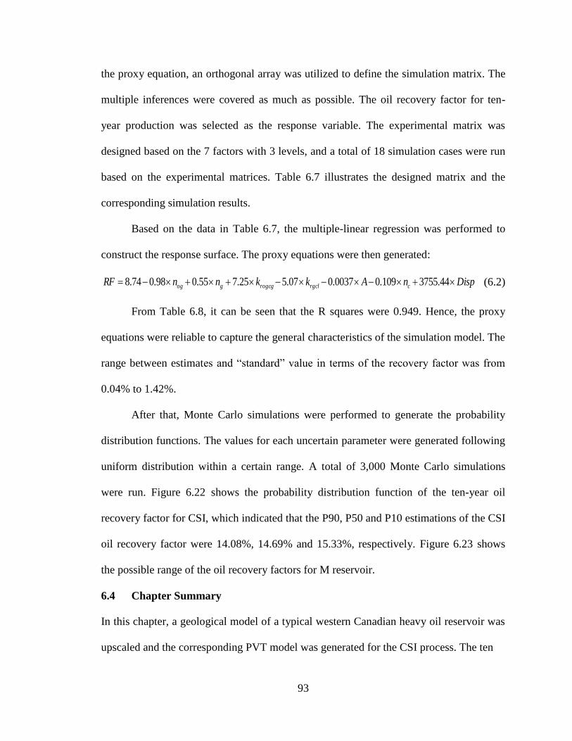
93
the proxy equation, an orthogonal array was utilized to define the simulation matrix. The
multiple inferences were covered as much as possible. The oil recovery factor for ten-
year production was selected as the response variable. The experimental matrix was
designed based on the 7 factors with 3 levels, and a total of 18 simulation cases were run
based on the experimental matrices. Table 6.7 illustrates the designed matrix and the
corresponding simulation results.
Based on the data in Table 6.7, the multiple-linear regression was performed to
construct the response surface. The proxy equations were then generated:
DispnAkknnRF crgclrogcggog 44.3755109.00037.007.525.755.098.074.8 (6.2)
From Table 6.8, it can be seen that the R squares were 0.949. Hence, the proxy
equations were reliable to capture the general characteristics of the simulation model. The
range between estimates and “standard” value in terms of the recovery factor was from
0.04% to 1.42%.
After that, Monte Carlo simulations were performed to generate the probability
distribution functions. The values for each uncertain parameter were generated following
uniform distribution within a certain range. A total of 3,000 Monte Carlo simulations
were run. Figure 6.22 shows the probability distribution function of the ten-year oil
recovery factor for CSI, which indicated that the P90, P50 and P10 estimations of the CSI
oil recovery factor were 14.08%, 14.69% and 15.33%, respectively. Figure 6.23 shows
the possible range of the oil recovery factors for M reservoir.
6.4 Chapter Summary
In this chapter, a geological model of a typical western Canadian heavy oil reservoir was
upscaled and the corresponding PVT model was generated for the CSI process. The ten
94
years’ primary production history (CHOPS) was history matched. Based on the tuned
model, the operations of the CSI process were investigated. At the end, an uncertainty
assessment was conducted. The P90, P50 and P10 estimations of the CSI oil recovery
factor were 14.08%, 14.69% and 15.33%, respectively. The results show that through
simulating experiments conducted with physical models with different scales, the
uncertainties in predicting the field-scale CSI performance can be significantly reduced.
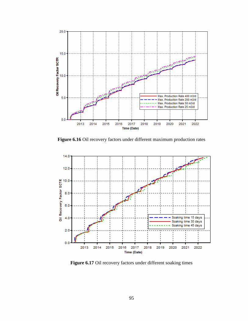
95
Figure 6.16 Oil recovery factors under different maximum production rates
Figure 6.17 Oil recovery factors under different soaking times
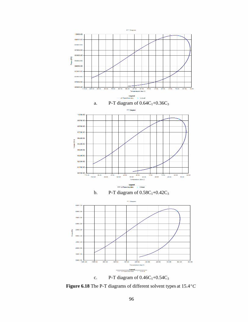
96
a. P-T diagram of 0.64C1+0.36C3
b. P-T diagram of 0.58C1+0.42C3
c. P-T diagram of 0.46C1+0.54C3
Figure 6.18 The P-T diagrams of different solvent types at 15.4 C
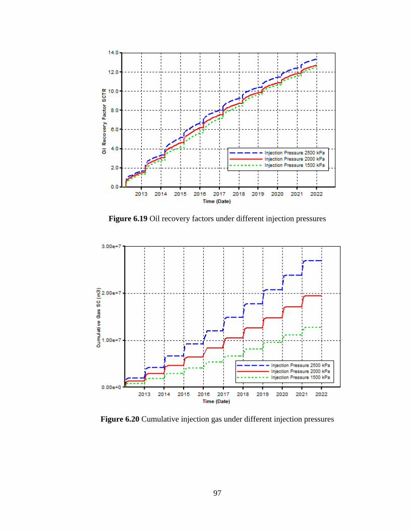
97
Figure 6.19 Oil recovery factors under different injection pressures
Figure 6.20 Cumulative injection gas under different injection pressures
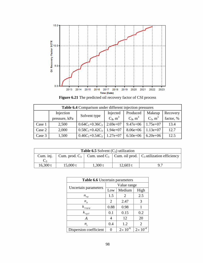
98
Figure 6.21 The predicted oil recovery factor of CSI process
Table 6.4 Comparison under different injection pressures
Injection
pressure, kPa Solvent type
Injected
C3, m3
Produced
C3, m3
Makeup
C3, m3
Recovery
factor, %
Case 1 2,500 0.64C1+0.36C3 2.69e+07 9.47e+06 1.75e+07 13.4
Case 2 2,000 0.58C1+0.42C3 1.94e+07 8.06e+06 1.13e+07 12.7
Case 3 1,500 0.46C1+0.54C3 1.27e+07 6.50e+06 6.20e+06 12.5
Table 6.5 Solvent (C3) utilization
Cum. inj.
C3
Cum. prod. C3 Cum. used C3 Cum. oil prod. C3 utilization efficiency
16,300 t 15,000 t 1,300 t 12,603 t 9.7
Table 6.6 Uncertain parameters
Uncertain parameters Value range
Low Medium High
ogn 1.5 2 2.5
gn 2 2.47 3
rogcgk 0.88 0.98 1
rgclk 0.1 0.15 0.2
A 4 12 20
cn 0.4 1.2 2
Dispersion coefficient 0 210-6
210-4
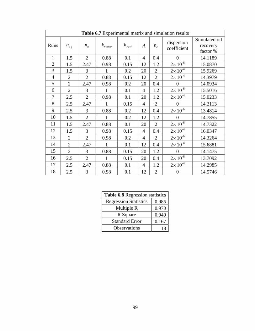
99
Table 6.7 Experimental matrix and simulation results
Runs gon gn rogcgk
rgclk A cn dispersion
coefficient
Simulated oil
recovery
factor %
1 1.5 2 0.88 0.1 4 0.4 0 14.1189
2 1.5 2.47 0.98 0.15 12 1.2 210-6
15.0870
3 1.5 3 1 0.2 20 2 210-4
15.9269
4 2 2 0.88 0.15 12 2 210-4
14.3979
5 2 2.47 0.98 0.2 20 0.4 0 14.0934
6 2 3 1 0.1 4 1.2 210-6
15.5016
7 2.5 2 0.98 0.1 20 1.2 210-4
15.0233
8 2.5 2.47 1 0.15 4 2 0 14.2113
9 2.5 3 0.88 0.2 12 0.4 210-6
13.4814
10 1.5 2 1 0.2 12 1.2 0 14.7855
11 1.5 2.47 0.88 0.1 20 2 210-6
14.7322
12 1.5 3 0.98 0.15 4 0.4 210-4
16.0347
13 2 2 0.98 0.2 4 2 210-6
14.3264
14 2 2.47 1 0.1 12 0.4 210-4
15.6881
15 2 3 0.88 0.15 20 1.2 0 14.1475
16 2.5 2 1 0.15 20 0.4 210-6
13.7092
17 2.5 2.47 0.88 0.1 4 1.2 210-4
14.2985
18 2.5 3 0.98 0.1 12 2 0 14.5746
Table 6.8 Regression statistics
Regression Statistics 0.985
Multiple R 0.970
R Square 0.949
Standard Error 0.167
Observations 18

100
Figure 6.22 Probability distribution of RF for CSI
Figure 6.23 Possible range of RF for M reservoir
0.00%
10.00%
20.00%
30.00%
40.00%
50.00%
60.00%
70.00%
80.00%
90.00%
100.00%
0
50
100
150
200
250
300
13
.09
13
.29
13
.50
13
.71
13
.91
14
.12
14
.33
14
.54
14
.74
14
.95
15
.16
15
.36
15
.57
15
.78
15
.99
Mo
re
Fre
qu
en
cy
group
Histogram
Frequency
0
2
4
6
8
10
12
14
16
RF,
%
Time
RF, %
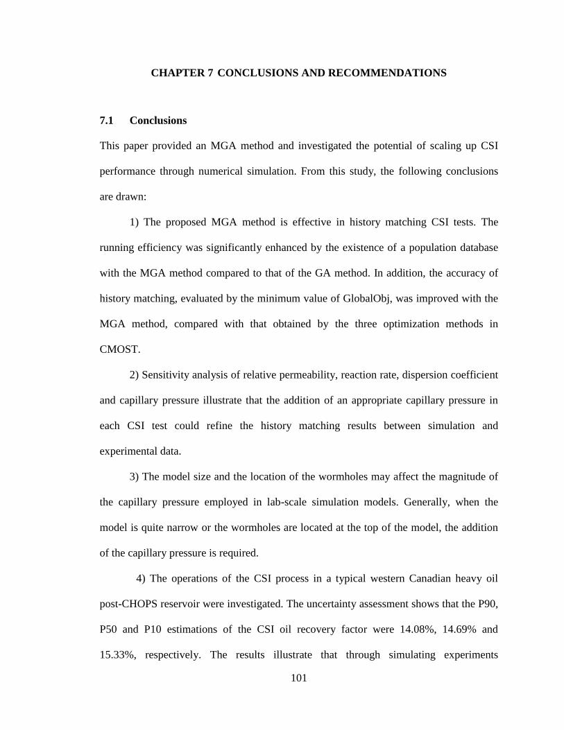
101
CHAPTER 7 CONCLUSIONS AND RECOMMENDATIONS
7.1 Conclusions
This paper provided an MGA method and investigated the potential of scaling up CSI
performance through numerical simulation. From this study, the following conclusions
are drawn:
1) The proposed MGA method is effective in history matching CSI tests. The
running efficiency was significantly enhanced by the existence of a population database
with the MGA method compared to that of the GA method. In addition, the accuracy of
history matching, evaluated by the minimum value of GlobalObj, was improved with the
MGA method, compared with that obtained by the three optimization methods in
CMOST.
2) Sensitivity analysis of relative permeability, reaction rate, dispersion coefficient
and capillary pressure illustrate that the addition of an appropriate capillary pressure in
each CSI test could refine the history matching results between simulation and
experimental data.
3) The model size and the location of the wormholes may affect the magnitude of
the capillary pressure employed in lab-scale simulation models. Generally, when the
model is quite narrow or the wormholes are located at the top of the model, the addition
of the capillary pressure is required.
4) The operations of the CSI process in a typical western Canadian heavy oil
post-CHOPS reservoir were investigated. The uncertainty assessment shows that the P90,
P50 and P10 estimations of the CSI oil recovery factor were 14.08%, 14.69% and
15.33%, respectively. The results illustrate that through simulating experiments

102
conducted with physical models with different scales, the uncertainties in predicting the
field-scale CSI performance can be significantly reduced.
7.2 Recommendations
The following recommendations are made for future work:
1) A different orthogonal array could be created to see whether it will affect the
history matching process significantly. The parameters in the GA toolbox could be
investigated for history matching the CSI process, such as using different crossover and
mutation functions.
2) A sensitivity analysis could be conducted before the history matching process,
in order to determine the overall variation of simulation results under different parameter
values and/or which parameters have the greatest effect on simulation results.
3) The foamy oil models in the CMG STARS could be investigated more. The
reasonable range of the frequency factor for the CSI process should be determined in a
future study.
4) A larger physical model could be used to conduct the CSI experiment, in order
to validate the reliability of predicting the upscaled CSI performance through numerical
simulation.
5) The proposed MGA method could be improved further by running cases in
parallel.
6) More wormhole structures in the field-scale simulation models could be formed
to investigate the effect of wormhole structure on CSI performance.
7) An economic analysis could be conducted for the investigation of field CSI
operational strategies.
103
REFERENCES
Ayub, M. and Tuhinuzzaman, M. 2007. The Role of Capillarity in the VAPEX Process.
Petroleum Society’s 8th Canadian International Petroleum Conference, Calgary,
Alberta, Canada.
Badamchizadeh, A., Maini, B.B., and Yarranton H. 2008. Applicability of CO2-Based
Vapex Process to Recover Athabasca Bitumen. International Thermal Operations and
Heavy Oil Symposium, Calgary, Alberta, Canada.
Bjorndalen, N., Jossy, W.E., and Alvarez, J.M. 2012. Foamy Oil Behaviour in Solvent
Based Production Processes. SPE Heavy Oil Conference, Calgary, Alberta, Canada.
Boustani, A. and Maini, B.B. 2001. The Role of Diffusion and Convective Dispersion in
Vapour Extraction Process. Journal of Canadian Petroleum Technology, 40(4), 68-
77.
Butler, R.M. and Mokrys, I.J. 1989. Solvent Analog Model Steam-assisted Drainage.
AOSTRA Journal of Research, 5(1), 17-32.
Butler, R.M. and Mokrys, I.J. 1991. A New Process (VAPEX) For Recovering Heavy
Oils Using Hot Water and Hydrocarbon Vapour. Journal of Canadian Petroleum
Technology, 30(1), 97-106.
Butler, R.M. and Mokrys, I.J. 1993. Recovery of Heavy Oils Using Vapourized
Hydrocarbon Solvents: Further Development of the Vapex Process. Journal of
Canadian Petroleum Technology, 32(6), 56-62.
Butler, R.M. and Jiang, Q. 2000. Improved Recovery of Heavy Oil by VAPEX with
Widely Spaced Horizontal Injector and Producer. Journal of Canadian Petroleum
Technology, 39(1), 48-56.
Castellini, A., Gullapalli, I., Hoang, V., and Condon, P. 2005. Quantifying Uncertainty in
Production Forecast for Fields with Significant History: a West African Case Study.
International Petroleum Technology Conference, Doha, Qatar.
Chamkalani, A., Zendehboudi, S., Chamkalani, R., Lohi, A., Elkamel, A., and Chatzis, I.
2013. Utilization of Support Vector Machine to Calculate Gas Compressibility
Factor. Fluid Phase Equilibria, 358, 189-202.
104
Chang, J. and Ivory, J. 2012. Field Scale Simulation of Cyclic Solvent Injection (CSI).
SPE Heavy Oil Conference, Calgary, Alberta, Canada.
Chipperfield, A., Fleming, P., Pohlheim, H., and Fonseca, C. 1994. The MATLAB
Genetic Algorithm Toolbox v1.2 User's Guide. University of Sheffield, UK.
Cuthiell, D., Kissel, G., Jackson, C., Frauenfeld, T., Fisher, D., and Rispler, K. 2006.
Viscous Fingering Effects in Solvent Displacement of Heavy Oil. Journal of
Canadian Petroleum Technology, 45 (7), 29-39.
Cuthiell, D., McCarthy, C., and Kissel, G. 2006. The Role of Capillarity in VAPEX.
Petroleum Society’s 7th Canadian International Petroleum Conference, Calgary,
Alberta, Canada.
Cuthiell, D. and Edmunds, N. 2012. Thoughts on Simulating the VAPEX Process. SPE
Heavy Oil Conference Canada, Calgary, Alberta, Canada.
Das, S.K. and Butler, R.M. 1998. Mechanism of the Vapor Extraction Process for Heavy
Oil and Bitumen. Journal of Petroleum Science Engineering, 21(1-2), 43-59.
Denbina, E.S., Baker, R.O., Gegunde, G.G., Klesken, A.J., and Sodero, S.F. 2001.
Modeling Cold Production for Heavy Oil Reservoirs. Journal of Canadian Petroleum
Technology, 40(3), 23-29.
Du, Z., Zeng, F., and Chan, C. 2013. An Experimental Study of the Post-CHOPS Cyclic
Solvent Injection Process. SPE Heavy Oil Conference Canada, Calgary, Alberta,
Canada.
Du, Z., Zeng, F., and Chan, C. 2014. Effect of Pressure Decline Rate on the Post-CHOPS
Cyclic Solvent Injection Process. SPE Heavy Oil Conference Canada, Calgary,
Alberta, Canada.
Firouz, Q. and Torabi, F. 2012. Feasibility Study of Solvent-Based Huff-n-Puff Method
(Cyclic Solvent Injection) to Enhance Heavy Oil Recovery. SPE Heavy Oil
Conference, Calgary, Alberta, Canada.
Frauenfeld, T.W.J., Kimber, K.D., and Sawatzky, R. 1994. A Partially Scaled Physical
Model of Cyclic Steam Stimulation for Recovery of Oil and Bitumen, SPE/DOE
Ninth Symposium on Improved Oil Recovery.
Grefenstette, J.J. 1986. Optimization of Control Parameters for Genetic Algorithms.
IEEE Transactions on Systems, Man and Cybernetics, 16(1), 122-128.
105
Holland, J. 1975. Adaptation in Natural and Artificial Systems. University of Michigan
Press, Ann Arbor.
Istchenko, C.M. and Gates, I.D. 2011. The Well-Wormhole Model of Cold Production of
Heavy Oil Reservoirs. SPE Heavy Oil Conference and Exhibition, Kuwait City,
Kuwait.
Istchenko, C.M. and Gates, I.D. 2012. The Well-Wormhole Model of CHOPS: History
Match and Validation. SPE Heavy Oil Conference Canada, Calgary, Alberta, Canada.
Ivory, J., Chang, J., Coates, R., and Forshner, K. 2010. Investigation of Cyclic Solvent
Injection Process for Heavy Oil Recovery. Journal of Canadian Petroleum
Technology, 49(9), 22-33.
Jamaloei, B.Y., Dong, M., Mahinpey, N., and Maini, B.B. 2012. Enhanced Cyclic
Solvent Process (ECSP) for Heavy Oil and Bitumen Recovery in Thin Reservoirs,
Energy & Fuels, 26, 2865-2874.
Jha, K.N., Butler, R.M., Lim, G.B., and Oballa, V. 1995. Proceedings of the 6th United
Nations Institute for Training and Research (UNITAR). International Conference;
Houston, TX.
Jiang, Q. 1997. Recovery of Heavy Oil and Bitumen Using Vapex Process in
Homogeneous and Heterogeneous Reservoir. Ph.D. Dissertation, University of
Calgary, Calgary, Alberta, Canada.
Kapadia, R.A. and Upreti, S.R. 2006. Determination of Gas Dispersion in Vapor
Extraction of Heavy Oil and Bitumen. Journal of Petroleum Science and
Engineering, 51(3-4), 214-222.
Karmaker, K. and Maini, B.B. 2003. Experimental Investigation of Oil Drainage Rates in
the Vapex Process for Heavy Oil and Bitumen Reservoirs. SPE Annual Technical
Conference and Exhibition held in Denver, Colorado, U.S.A.
Kumar, K.V. 2009. Neural Network Prediction of Interfacial Tension at Crystal/Solution
Interface. Industrial & Engineering Chemical Research, 48(8), 4160-4164.
Kumar, R. and Darvish M.P. 2003. Solution-Gas Drive in Heavy Oil: Field Prediction
and Sensitivity Studies using Low Gas Relative Permeability. Journal of Canadian
Petroleum Technology, 41(3), 26-32.
106
Lau, E. 2001. An Integrated Approach to Understand Cold Production Mechanisms of
Heavy Oil Reservoirs. Canadian International Petroleum Conference, Calgary,
Alberta, Canada.
Li, R., Reynolds, A.C., and Oliver, D.S. 2001. History Matching of Three-phase Flow
Production Data. SPE Reservoir Simulation Symposium, Houston, Texas.
Lim, G.B., Kry, R.P., Harker, B.C., and Jha, K.N. 1995. Cyclic Stimulation of Cold Lake
Oil Sand with Supercritical Ethane. International Heavy Oil Symposium, Calgary,
Alberta, Canada.
Lim, G.B., Kry, R.P., Harker, B.C., and Jha, K.N. 1996. Three-dimensional Scaled
Physical Modeling of Solvent Vapour Extraction of Cold Lake Bitumen. Journal of
Canadian Petroleum Technology, 35 (4), 32-40.
Liu, X. and Zhao, G. 2003. A Fractal Wormhole Model for Cold Heavy Oil Production.
Canadian International Petroleum Conference, Calgary, AB, June 10 - 12, 2003.
Loughead, D.J. and Saltuklaroglu, M. 1992. Lloydminster Heavy Oil Production-Why So
Unusual? The 9th
Annual Heavy Oil and Oil Sand Technology Symposium, Calgary,
Alberta, Canada.
Maini, B.B. 2001. Foamy-Oil Flow. Journal of Petroleum Technology, 53(10), 54-64.
Mantica, S., Cominelli, A., and Mantica, G. 2001. Combining Global and Local
Techniques for Automatic History Matching Production and Seismic Data. SPE
Reservoir Simulation Symposium, Houston, Texas.
Metwally, M. and Solanki, S.C. 1995. Heavy Oil Reservoir Mechanisms, Lindbergh, and
Frog Lake Fields, Alberta, Part I: Field Observations and Reservoir Simulation.
Annual Technical Meeting of the Petroleum Society, Banff, Alberta, Canada.
Mitchell, M. 1996. An Introduction to Genetic Algorithms. Massachusetts: MIT Press.
Nenniger, J.E. and Dunn, S.G. 2008. How Fast is Solvent Based Gravity Drainage?
Canadian International Petroleum Conference/SPE Gas Technology Symposium,
Calgary, Alberta, Canada.
Reynolds, A.C., Li, R., and Oliver, D.S. 2004. Simultaneous Estimation of Absolute and
Relative Permeability by Automatic History Matching of Three-phase Flow
Production Data. Journal of Canadian Petroleum Technology, 43(3), 37-46.
107
Roosta, A., Setoodeh, P., and Jahanmiri A. 2012. Artificial Neural Network Modeling of
Surface Tension for Pure Organic Compounds. Industrial & Engineering Chemical
Research, 51(1), 561-566.
Sampaio, T.P., Ferreira Filho, V.J.M., and de Sa Neto, A. 2009. An Application of Feed
Forward Neural Network as Nonlinear Proxies for the Use during the History
Matching Phase. SPE Latin American and Caribbean Petroleum Engineering
Conference, Cartagena, Colombia.
Sawatzky, R.P., Lillico, D.A., London, M.J., and Tremblay, B. 2002. Tracking Cold
Production Footprints. Petroleum Society’s Canadian International Petroleum
Conference 2002, Calgary, Alberta, Canada.
Schulze-Riegert, R.W., Axmann, J.K., Haase, O., and Rian, D.T. 2002. Evolutionary
Algorithms Applied to History Matching of Complex Reservoirs. SPE Reservoir
Evaluation & Engineering, 5(2), 163-173.
Shafiei, A., Dusseault, M.B., Zendehboudi, S., and Chatzis, I. 2013. A New Screening
Tool for Evaluation of Steamflooding Performance in Naturally Fractured Carbonate
Reservoirs. Fuel, 108, 502-514.
Silva, P.C., Maschio, C., and Schiozer, D.J. 2006. Applications of the Soft Computing in
the Automated History Matching. Canadian International Petroleum Conference,
Calgary, Alberta, Canada.
Squires, A. 1993. Inter-Well Tracer Results and Gel Blocking Program. 10th Annual
Heavy Oil and Oil Sands Technical Symposium, Calgary, Alberta, Canada.
Sultan, A.J., Ouenes, A., and Weiss, W.W. 1994. Automatic History Matching for an
Integrated Reservoir Description and Improving Oil Recovery. Permian Basin Oil and
Gas Recovery Conference, Midland, Texas.
Sun, X. and Mohanty, K.K. 2005. Estimation of Flow Functions during Drainage using
Genetic Algorithm. SPE Journal, 10(4), 449-457.
Tan, T.B. and Kalogerakis, N. 1992. A Three-dimensional Three-phase Automatic
History Matching Model: Reliability of Parameter Estimates. Journal of Canadian
Petroleum Technology, 31(3), 34-41.
108
Tan, T., Slevinsky, R., and Jonasson, H. 2003. A New Methodology for Modeling of
Sand Wormholes in Field Scale Thermal Simulations. Canadian International
Petroleum Conference, Calgary, Alberta, Canada.
Tasrief, M. and Kashiwagi, M. 2013. Improvement of Ship Geometry by Optimizing the
Sectional Area Curve with Binary-Coded Genetic Algorithms (BCGAs). Twenty-
third International Offshore and Polar Engineering, Anchorage, Alaska, USA.
Thomas, L.K., Hellums, L.J., and Rehais, G. M. 1972. A Nonlinear Automatic History
Matching Technique for Reservoir Simulation Models. Society of Petroleum
Engineers Journal, 12(6), 508-514.
Tremblay, B. 2009. Cold flow: A Multi-well Cold Production (CHOPS) Model. Journal
of Canadian Petroleum Technology, 48(2), 22-28.
Tremblay, B., Sedgwick, G., and Vu, D. 1999. A Review of Cold Production. EAGE-
10th European Symposium on Improved Oil Recovery, Brighton, UK.
Wang, Y. and Chen, C.Z. 2004. Simulating Cold Heavy-Oil Production with Sand by
Reservoir-Wormhole Model. Journal of Canadian Petroleum Technology, 43(4), 39-
44.
Wathiq J.A. 2013. Coupling Programming of an Adaptive Genetic Algorithm with
Reservoir Flow Simulation for Infill Oil Well Location Optimization. SPE Western
Regional & AAPG Pacific Section Meeting, Monterey, California, USA.
WinProp User’s Guide, Phase-behavior and Fluid Property Program, Version 2012, by
Computer Modelling Group Ltd.
Xu, S., Zeng, F., Gu, Y., and Knorr, K. 2012. Upscaling Study of Vapour Extraction
Process through Numerical Simulation. SPE Heavy Oil Conference, Calgary, Alberta,
Canada.
Yang, C., Nghiem, L.X., Card, C., and Bremeier, M. 2007. Reservoir Model Uncertainty
Quantification through Computer-Assisted History Matching. SPE Annual Technical
Conference and Exhibition, Anaheim, California, USA.
Yang, P.H. and Watson, A.T. 1991. A Bayesian Methodology for Estimating Relative
Permeability Curves. SPE Reservoir Engineering, 6(2), 259-265.
109
Yazdani, A., and Maini, B.B. 2005. Effect of Drainage Height and Grain Size on
Production Rates in the VAPEX Process: Experimental Study. SPE Reservoir
Evaluation & Engineering, 8(3), 205-213.
Yazdani, A. and Maini, B.B. 2009. Pitfalls and Solutions in Numerical Simulation of
VAPEX Experiments, Energy & Fuels, 23, 3981-3988.
Yuan, J.Y., Tremblay, B., and Babchin, A. 1999. A Wormhole Network Model of Cold
Production in Heavy Oil. International Thermal Operations/Heavy Oil Symposium,
Bakersfield, California.
Zeng, F., Knorr, K.D., and Wilton, R. 2008. Post-Cold Production Solvent Vapor
Extraction (SVX) Process Performance Evaluation by Numerical Simulation.
Canadian International Petroleum Conference, Calgary, Alberta, Canada.
110
APPENDIX A
THE CODE FOR AUTOMATIC HISTORY MATCHING COMBINED DESIGN
OF EXPERIMENTS METHOD AND GENETIC ALGORITHM
function main
CMG_callback(); [RF_final]=read_rwofile(); [exptime expRF expCumGas]=Read_experiment_data(); [initial_pop]=Objfunction_cal(exptime,expRF,RF_final);
end
111
function CMG_callback()
row=25;
for r=1:row-1
s1=['D:\GA\GA codes_2014 CSI_test 4\','2014 CSI test4_',num2str(r),'.dat'];
movefile(s1,'D:\GA\GA codes_2014 CSI_test 4\proxy_cases');
s5=['D:\GA\GA codes_2014 CSI_test 4\proxy_cases\2014 CSI test4_',num2str(r),'.dat'];
copyfile(s5, 'D:\GA\GA codes_2014 CSI_test 4');
s6=['2014 CSI test4_',num2str(r),'.dat'];
s7=['2014 CSI test4_',num2str(r+1),'.dat'];
movefile(s6,s7);
end
for r=1:row-1
s8=['D:\GA\GA codes_2014 CSI_test 4\proxy_cases\','2014 CSI test4_',num2str(r),'.dat'];
movefile(s8,'D:\GA\GA codes_2014 CSI_test 4');
end
for r=1:row
fid = fopen('D:\GA\GA codes_2014 CSI_test 4\DOE.txt');
D=zeros(25,6);
D=textscan(fid,'%f %f %f %f %f %f');
fclose(fid);
rgcl=D{1};
g=D{2};
rogcg=D{3};
o=D{4};
a=D{5};
c=D{6};
krogcg=rogcg(r);
ng=g(r);
krgcl=rgcl(r);
nog=o(r);
A=a(r);
nc=c(r);
[kpg,krow]= Generate_perm_pc(krgcl,ng,krogcg,nog,A,nc);
Modify_perm_pc(kpg,krow,r);
end
matlabpool open 3;
t1=clock;
parfor r=1:row
s=['"C:\Program Files (x86)\CMG\STARS\2011.10\Win_x64\EXE\st201110.exe"',' -f
','"D:\GA\GA codes_2014 CSI_test 4\2014 CSI test4_',num2str(r),'.dat"'];
system(s);
end
disp(['etime:',num2str(etime(clock,t1)/60/60)]);
end
112
function [RF_final]=read_rwofile()
row=25;
for r=1:8
s1=['D:\GA\GA codes_2014 CSI_test 4\report',num2str(r),'.rwd'];
movefile(s1,'D:\GA\GA codes_2014 CSI_test 4\proxy_cases');
s5=['D:\GA\GA codes_2014 CSI_test 4\proxy_cases\report',num2str(r),'.rwd'];
copyfile(s5, 'D:\GA\GA codes_2014 CSI_test 4');
s6=['report',num2str(r),'.rwd'];
s7=['report',num2str(r+1),'.rwd'];
movefile(s6,s7);
end
r=9;
s1=['D:\GA\GA codes_2014 CSI_test 4\report',num2str(r),'.rwd'];
movefile(s1,'D:\GA\GA codes_2014 CSI_test 4\proxy_cases');
for r=10:row-1
s1=['D:\GA\GA codes_2014 CSI_test 4\report',num2str(r),'.rwd'];
movefile(s1,'D:\GA\GA codes_2014 CSI_test 4\proxy_cases');
%copy .dat file back from proxy_cases folder to the upper folder
s5=['D:\GA\GA codes_2014 CSI_test 4\proxy_cases\report',num2str(r),'.rwd'];
copyfile(s5, 'D:\GA\GA codes_2014 CSI_test 4');
%change the name of the current .dat file to next .dat file.
s6=['report',num2str(r),'.rwd'];
s7=['report',num2str(r+1),'.rwd'];
movefile(s6,s7);
end
for r=1:row-1
s8=['D:\GA\GA codes_2014 CSI_test 4\proxy_cases\report',num2str(r),'.rwd'];
movefile(s8,'D:\GA\GA codes_2014 CSI_test 4');
end
for r=1:9
r1=['D:\GA\GA codes_2014 CSI_test 4\report',num2str(r),'.rwd'];
fid=fopen(r1,'r+');
fseek(fid,25,-1); %locate put the point at the beginning of the data
fprintf(fid,'%1.0f',r);
fclose(fid);
end
for r=10:row
r1=['D:\GA\GA codes_2014 CSI_test 4\report',num2str(r),'.rwd'];
fid=fopen(r1,'r+');
fseek(fid,25,-1); %locate put the point at the beginning of the data
fprintf(fid,'%1.0f',r);
fclose(fid);
end
for r=1:row
113
s=['"C:\Program Files (x86)\CMG\BR\2011.10\Win_x64\EXE\report.exe"',' -f
','"D:\GA\GA codes_2014 CSI_test 4\report',num2str(r),'.rwd"',' -o ','"D:\GA\GA
codes_2014 CSI_test 4\report',num2str(r),'.rwo"'];
system(s);
r2=['D:\GA\GA codes_2014 CSI_test 4\report',num2str(r),'.rwo'];
fid = fopen(r2,'r+');
S=textscan(fid,'%f %f','headerlines',13);
simtime=zeros(length(S{1,1}),row);
simRF=zeros(length(S{1,1}),row);
simtime(:,r)=S{1,1}/60/24;
simRF(:,r)=S{1,2};
fclose(fid);
RF_final(r)=max(simRF(:,r));
end
end
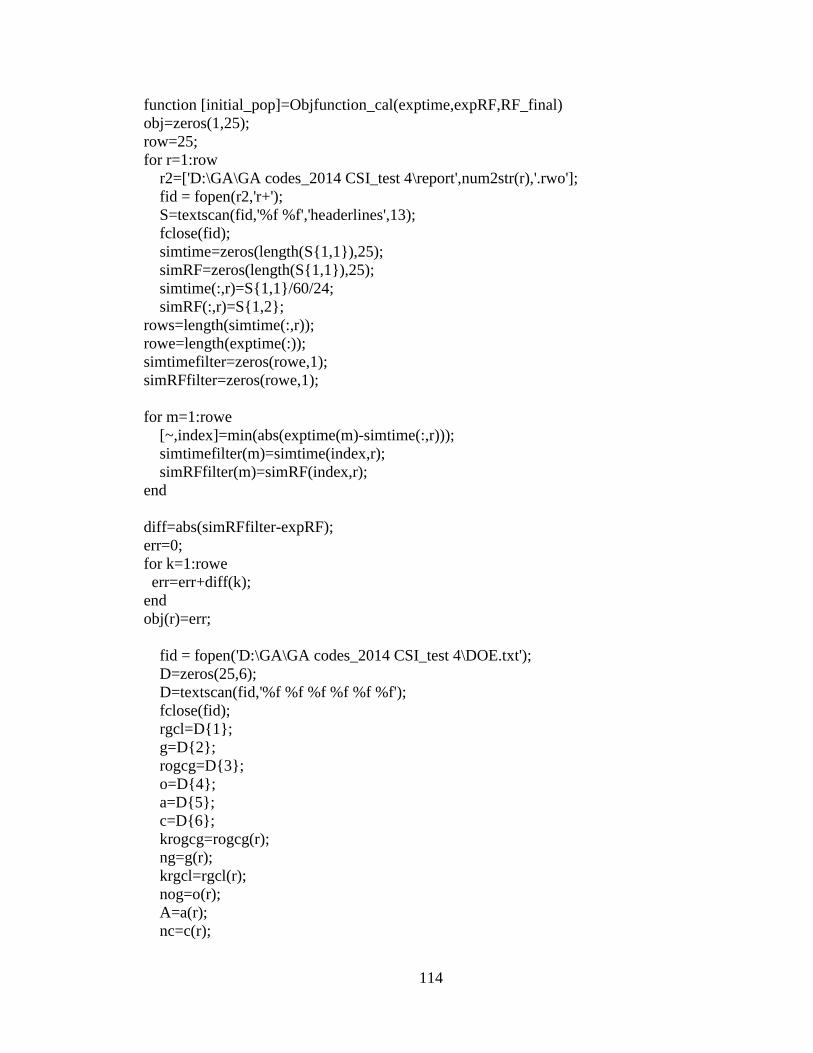
114
function [initial_pop]=Objfunction_cal(exptime,expRF,RF_final)
obj=zeros(1,25);
row=25;
for r=1:row
r2=['D:\GA\GA codes_2014 CSI_test 4\report',num2str(r),'.rwo'];
fid = fopen(r2,'r+');
S=textscan(fid,'%f %f','headerlines',13);
fclose(fid);
simtime=zeros(length(S{1,1}),25);
simRF=zeros(length(S{1,1}),25);
simtime(:,r)=S{1,1}/60/24;
simRF(:,r)=S{1,2};
rows=length(simtime(:,r));
rowe=length(exptime(:));
simtimefilter=zeros(rowe,1);
simRFfilter=zeros(rowe,1);
for m=1:rowe
[~,index]=min(abs(exptime(m)-simtime(:,r)));
simtimefilter(m)=simtime(index,r);
simRFfilter(m)=simRF(index,r);
end
diff=abs(simRFfilter-expRF);
err=0;
for k=1:rowe
err=err+diff(k);
end
obj(r)=err;
fid = fopen('D:\GA\GA codes_2014 CSI_test 4\DOE.txt');
D=zeros(25,6);
D=textscan(fid,'%f %f %f %f %f %f');
fclose(fid);
rgcl=D{1};
g=D{2};
rogcg=D{3};
o=D{4};
a=D{5};
c=D{6};
krogcg=rogcg(r);
ng=g(r);
krgcl=rgcl(r);
nog=o(r);
A=a(r);
nc=c(r);

115
rec=[krgcl ng krogcg nog A nc RF_final(r) obj(r)];
dlmwrite('DOEscore.txt', rec, '-append','delimiter', '\t','newline','pc');
end
[~,index]=min(obj);
row=index;
fid = fopen('D:\GA\GA codes_2014 CSI_test 4\DOE.txt');
D=zeros(25,6);
D=textscan(fid,'%f %f %f %f %f %f');
fclose(fid);
rgcl=D{1};
g=D{2};
rogcg=D{3};
o=D{4};
a=D{5};
c=D{6};
krogcg=rogcg(row);
ng=g(row);
krgcl=rgcl(row);
nog=o(row);
A=a(row);
nc=c(row);
initial_pop=[krgcl ng krogcg nog A nc];
disp(['the initial population could be:',num2str(initial_pop)]);
end
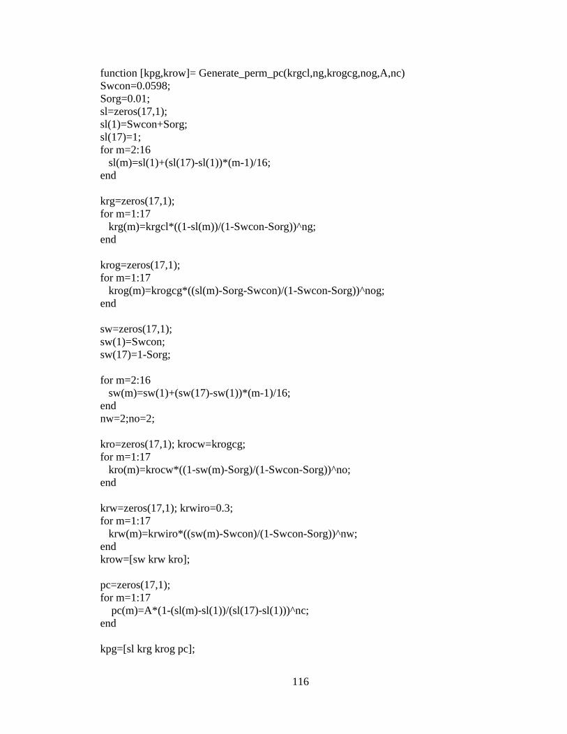
116
function [kpg,krow]= Generate_perm_pc(krgcl,ng,krogcg,nog,A,nc)
Swcon=0.0598;
Sorg=0.01;
sl=zeros(17,1);
sl(1)=Swcon+Sorg;
sl(17)=1;
for m=2:16
sl(m)=sl(1)+(sl(17)-sl(1))*(m-1)/16;
end
krg=zeros(17,1);
for m=1:17
krg(m)=krgcl*((1-sl(m))/(1-Swcon-Sorg))^ng;
end
krog=zeros(17,1);
for m=1:17
krog(m)=krogcg*((sl(m)-Sorg-Swcon)/(1-Swcon-Sorg))^nog;
end
sw=zeros(17,1);
sw(1)=Swcon;
sw(17)=1-Sorg;
for m=2:16
sw(m)=sw(1)+(sw(17)-sw(1))*(m-1)/16;
end
nw=2;no=2;
kro=zeros(17,1); krocw=krogcg;
for m=1:17
kro(m)=krocw*((1-sw(m)-Sorg)/(1-Swcon-Sorg))^no;
end
krw=zeros(17,1); krwiro=0.3;
for m=1:17
krw(m)=krwiro*((sw(m)-Swcon)/(1-Swcon-Sorg))^nw;
end
krow=[sw krw kro];
pc=zeros(17,1);
for m=1:17
pc(m)=A*(1-(sl(m)-sl(1))/(sl(17)-sl(1)))^nc;
end
kpg=[sl krg krog pc];

117
function Modify_kr_pc(kpg,krow)
[fid] = fopen('D:\GA\GA codes_2014 CSI_test 5\2014 CSI test5.dat',r+');
sread=fscanf(fid,'%c'); k=strfind(sread, 'SWT'); fseek(fid,k+2,-1);
for m=1:17 fprintf(fid,'\r\n %6.4f %12.10f %12.10f',krow(m,1),krow(m,2),krow(m,3)); end k=strfind(sread, 'SLT');
fseek(fid,k+2,-1);
for m=1:17 fprintf(fid,'\r\n %6.4f %12.10f %12.10f %12.10f',kpg(m,1),kpg(m,2),kpg(m,3),kpg(
m,4)); end fclose(fid);

118
function [simtime simRF RF_final]=CMG_call()
system('"C:\Program Files x86)\CMG\STARS\2011.10\Win_x64\EXE\st201110.exe" -f
"D:\GA\GA codes_2014 CSI_test 5\2014 CSI test5.dat"'); system('"C:\Program Files (x86)\CMG\BR\2011.10\Win_x64\EXE\report.exe" -f
"D:\GA\GA codes_2014 CSI_test 5\report.rwd" -o "D:\GA\GA codes_2014 CSI_test
5\report.rwo"'); fid = fopen('D:\GA\GA codes_2014 CSI_test 5\report.rwo'); S=textscan(fid,'%f %f','headerlines',13); simtime=S{1}/60/24; simRF=S{2}; RF_final=max(simRF); fclose(fid); end

119
function [exptime expRF expCumGas]=Read_experiment_data()
fid = fopen('D:\GA\GA codes_2014 CSI_test 5\2014 CSI test5.fhf');
E=zeros(27,4);
E=textscan(fid,'%f %f %f %f','headerlines',9);
exptime=E{1};
expRF=E{3};
expCumGas=E{4};
fclose(fid);

120
function obj=Objfunction_calculation(simtime,simRF,exptime,expRF)
rows=length(simtime);
rowe=length(exptime);
simtimefilter=zeros(rowe,1);
simRFfilter=zeros(rowe,1);
for m=1:rowe
[~,index]=min(abs(exptime(m)-simtime(:)));
simtimefilter(m)=simtime(index);
simRFfilter(m)=simRF(index);
end
diff=abs(simRFfilter-expRF);
obj=0;
for k=1:rowe;
obj=obj+diff(k);
end
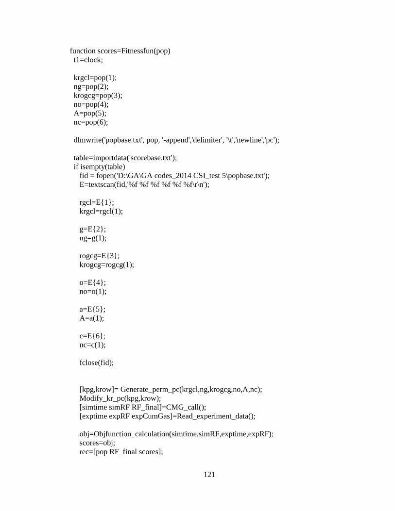
121
function scores=Fitnessfun(pop)
t1=clock;
krgcl=pop(1);
ng=pop(2);
krogcg=pop(3);
no=pop(4);
A=pop(5);
nc=pop(6);
dlmwrite('popbase.txt', pop, '-append','delimiter', '\t','newline','pc');
table=importdata('scorebase.txt');
if isempty(table)
fid = fopen('D:\GA\GA codes_2014 CSI_test 5\popbase.txt');
E=textscan(fid,'%f %f %f %f %f %f\r\n');
rgcl=E{1};
krgcl=rgcl(1);
g=E{2};
ng=g(1);
rogcg=E{3};
krogcg=rogcg(1);
o=E{4};
no=o(1);
a=E{5};
A=a(1);
c=E{6};
nc=c(1);
fclose(fid);
[kpg,krow]= Generate_perm_pc(krgcl,ng,krogcg,no,A,nc);
Modify_kr_pc(kpg,krow);
[simtime simRF RF_final]=CMG_call();
[exptime expRF expCumGas]=Read_experiment_data();
obj=Objfunction_calculation(simtime,simRF,exptime,expRF);
scores=obj;
rec=[pop RF_final scores];
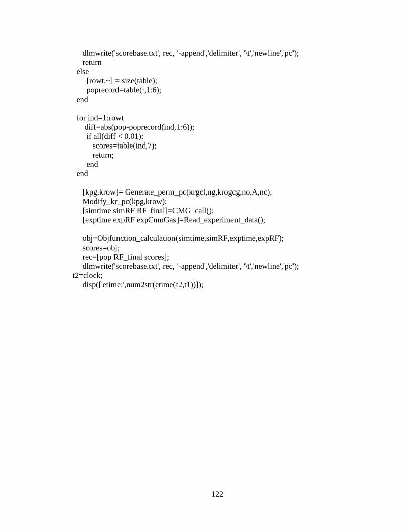
122
dlmwrite('scorebase.txt', rec, '-append','delimiter', '\t','newline','pc');
return
else
[rowt,~] = size(table);
poprecord=table(:,1:6);
end
for ind=1:rowt
diff=abs(pop-poprecord(ind,1:6));
if all(diff < 0.01);
scores=table(ind,7);
return;
end
end
[kpg,krow]= Generate_perm_pc(krgcl,ng,krogcg,no,A,nc);
Modify_kr_pc(kpg,krow);
[simtime simRF RF_final]=CMG_call();
[exptime expRF expCumGas]=Read_experiment_data();
obj=Objfunction_calculation(simtime,simRF,exptime,expRF);
scores=obj;
rec=[pop RF_final scores];
dlmwrite('scorebase.txt', rec, '-append','delimiter', '\t','newline','pc');
t2=clock;
disp(['etime:',num2str(etime(t2,t1))]);