lable at ScienceDirect

Polymer 51 (2010) 1432–1436

Contents lists avai

Polymer

journal homepage: www.elsevier .com/locate/polymer

A novel approach to predict the recovery time of shape memory polymers

M. Bonner a, H. Montes de Oca b, M. Brown b, I.M. Ward a,*

a School of Physics & Astronomy, The University of Leeds, Leads LS2 9JT, UKb Smith & Nephew, Group Research Centre, York Science Park, Heslington, York, YO10 5DF, UK

a r t i c l e i n f o

Article history:Received 15 October 2009Received in revised form22 January 2010Accepted 25 January 2010Available online 2 February 2010

Keywords:Shape memory polymerPolymer physicsRecovery

* Corresponding author. Tel.: þ44 113 343 3808; faE-mail address: i.m.ward@leeds.ac.uk (I.M. Ward).

0032-3861/$ – see front matter � 2010 Elsevier Ltd.doi:10.1016/j.polymer.2010.01.058

a b s t r a c t

In this paper a novel approach is presented for prediction of the recovery time for a shape memorypolymer. The Transient Stress Dip Tests of Fotheringham and Cherry are used to determine the twoparameters of a Kelvin–Voigt element. The characteristic retardation time of this element can then becalculated to predict the recovery time. It is shown that this approach is successful in predicting therecovery times for a shape memory polymer drawn and recovered under a range of temperatures.Furthermore it is shown that the ratio of the recovery stress to the draw stress is independent of thedrawing conditions to a very good approximation.

� 2010 Elsevier Ltd. All rights reserved.

1. Introduction

Recently there has been a surge of interest in shape recoveringpolymers and the community has adopted the term shape memorypolymers (SMP). A review of the recent progress in SMP and someof their applications in medical and non-medical industries can befound elsewhere [1–3].

Several models have been proposed to describe the behaviour ofSMPs, with two of the most recent being by proposed by Nguyen [4]and Chen [5,6], however these rely on constitutive equations andare hence quite complex and require significant experimental workto determine the relevant parameters.

The earlier work of Li and Larock [7] and Lin and Chen [8,9]proposed simpler models based on varying combinations ofMaxwell and Kelvin–Voigt elements. These are easy to understandmodels, all of which can under the right circumstances collapse toa single Kelvin or Voigt element.

In this work we present a novel approach to predict the shaperecovery time on the basis of a simple Kelvin–Voigt model shownin Fig. 1, using the transient stress dip tests of Fotheringham andCherry [9] to determine the stress in each arm under a range ofdrawing conditions and hence calculate both the recovery time ofthe material and the recovery stress available. We also investi-gate the effect of processing conditions on the recovery stress ofSMPs.

x: þ44 113 343 3846.

All rights reserved.

2. Theory

It is possible to use the Kelvin–Voigt model shown in Fig. 1 todescribe with a good degree of accuracy the behaviour of a visco-elastic material such as a solid polymer above the glass transitiontemperature. In this model the forward flow stress is given by thecombined stress in the two arms. For the shape recovery we assumethat the stress is stored in the spring ER during the drawing process.This element drives the dashpot hR backwards, resulting in thematerial returning to its original dimensions like a rubber band. Thetotal applied stress (sT) on the system is the sum of the stress in thetwo arms, thus

sT ¼ sR þ sn (1)

where sR is the recovery stress (the stress in the spring ER) and sv isthe viscosity stress, the stress in the dashpot hR.

This model is characterised by a recovery half life s which issimply given by [10]

s ¼ hR

ER(2)

where s is the recovery half life, hR is the viscosity of the dashpotand ER is the modulus of the spring. This recovery time is a half life,and so in order to predict the actual recovery time we need to addtogether seven of these half lives to achieve a recovery of over 99%,since s1 is the time required to recover to half of the initial exten-sion, s2 is the time required for half the remaining extension (equalto one quarter of the original extension) to recover, s3 is the time

Dashpotr

SpringE r

Fig. 1. Kelvin–Voigt model.

M. Bonner et al. / Polymer 51 (2010) 1432–1436 1433

required for half the remaining extension (equal to one eighth ofthe original extension) to recover and so on. By adding together 7 ofthese half lives we obtain a total recovery of 99.2%.

In the first instance, in order to simplify the procedure, we willassume that we can simply multiply the recovery time by 7 topredict the overall recovery time (since to calculate the individualhalf recovery times would require data to be collected over a verywide range of conditions). Thus if a technique is available thatallows the stress on the two arms to be determined then therecovery time can be calculated. We propose that the TransientStress Dip Tests of Fotheringham and Cherry [9] are a suitabletechnique to separate the stresses on the two arms. In these testsa sudden and rapid reduction is strain is used to probe the stresslevel on the spring by observing the resulting behaviour of the loadonce the sample is held at constant strain. Because the total stressin the system is the sum of the stresses on the two arms it is thenstraight forward to calculate the stress on the dashpot. There arethree possible situations schematically shown in Fig. 2 that canarise after the strain reduction has taken place.

i. sT > sR: In this case sv is positive and the stress reduces overtime as the dashpot flows.

ii. sT < sR: In this case sv is negative and the stress increasesover time as the dashpot flows.

iii. sT ¼ sR: In this case the strain rate in the dashpot is zero andthe stress initially remains constant with time.

Time

T R >

T

T

R =

R <

Load

Fig. 2. Schematic representation of the three possible behaviours that can occurduring the transient stress dip test.

Thus once sR has been determined ER and hR can be determinedusing the following equations:

ER ¼sR

3(3)

and

hR ¼sv

_3(4)

It is also apparent that for this approach to work the inherent stressrelaxation of the material must be long compared to the shaperecovery time. To confirm this, stress relaxation experiments werealso performed.

3. Experimental methods

3.1. Materials

The material used in this work was based on an amorphouslactide based copolymer with 35% weight of calcium carbonatesupplied by Smith & Nephew, York, in pellet form. This was con-verted to monofilament by using a bench scale melt spinningdevice attached to an Instron 5502. The spinning temperature was160 �C, the die had an exit diameter of 2 mm and the crosshead wasset to 2 mm per minute. The filament was spun into air at a rate ofapproximately 1 m per minute and allowed to coil into a clean trayfor collection. There was a gap of approximately 1 m between theoutput of the die and the tray. This produced a monofilament ofapproximately 1 mm diameter. Because the material used degradesin the presence of water both the pellets and the monofilamentwere kept under vacuum when not being tested.

3.2. Initial drawing

Initial drawing experiments were performed to determinesuitable conditions for later tests and also to ensure that thematerial exhibited suitable performance (i.e. complete recovery).These tests were performed on an Instron model 5502 using a longtravel Instron environmental chamber to provide elevatedtemperature conditions. Drawing was performed over a range oftemperatures (from 20 �C to 80 �C) and draw ratios (up to drawratio 7).

3.3. Transient stress dip tests

Transient stress dip tests were performed on an Instron model4505 utilising the advanced stress–strain panel to program thetests. The load output data from the Instron was monitored bya Pico ADC 200 linked to a laptop PC using Picolog software torecord the data. In these tests a sample of length 75 mm (themaximum length possible for the sample to reach l ¼ 4 withinthe travel available in the oven) is extended under conditions ofknown crosshead displacement rate (equivalent to a nominalstrain rate of 8.33 � 10�3 s�1) to a predetermined strain (in thiscase up to a maximum of l ¼ 4). At this strain the crosshead isreversed a small amount at a strain rate that is at least 10 timesthat of the forward strain rate. Once the small amount ofrecovery has taken place the crosshead is held stationary and theload output is monitored as a function of time. The load wasmonitored until it was clear what behaviour the load wasexhibiting. The tests were performed at elevated temperature byusing an environmental chamber capable of controlling thetemperature to �2 �C.

0

10

20

30

40

50

60

0 2 4 6 8 10 12

Reco

very S

tress (M

Pa)

λ2-λ-1

Fig. 4. Recovery stress against l2 � 1=l under tensile drawing at 55 �C and 65 �C.(Experimental data A 55 �C, linear fit - - 55 �C, experimental data - 65 �C, linear fit –65 �C).

M. Bonner et al. / Polymer 51 (2010) 1432–14361434

3.4. Shape recovery tests

Recovery tests were performed on a dead loading creep rig(shown in Fig. 3), the output of which was monitored by computerusing a data logging program written at Leeds. Samples for testingwere prepared by drawing under the same conditions as for thetransient stress dip tests (draw temperatures of 55–75 �C at a strainrate of 8.33 � 10�3 s�1) to a draw ratio of l ¼ 4. The samples wereprepared at least 24 h prior to the shape recovery tests beingperformed. Initial gauge lengths for the samples were between80 mm and 100 mm. The environmental chamber was heated to thetarget temperature as quickly as possible (it took approximately200 s from the start of the test for the air temperature in thechamber to achieve the set temperature) and held at the testtemperature until the test was complete. The test was determinedto be complete once the strain ceased to decrease and started toincrease (i.e. once all the energy stored in the spring had beenexpended in recovery and the sample returned to an essentiallyisotropic state and started to creep in the normal manner).

3.5. Stress relaxation

Stress relaxation experiments were performed on an Instronmodel 5545. Isotropic samples were gripped and extended underconditions that were the same as those used for the transient stressdip tests. Once the sample reached l ¼ 4 (as determined bycrosshead displacement) the crosshead was stopped and heldstationary, whilst the load continued to be monitored.

4. Results and discussion

4.1. Initial results

It was found that for optimum shape memory performance to beobserved (i.e. for near total recovery to be observed) then drawing

Fixed Upper Plate

Top Grip

Sample

Transducer Body

Lower Grip and Transducer Core Assembly

Fig. 3. Schematic diagram of a dead loading creep rig.

temperatures of between 55 �C and 75 �C were required anda maximum draw ratio of l ¼ 4 could be imposed. Because of thisfor shape memory recovery tests were performed at a draw ratio ofl ¼ 4, and transient stress dip tests were performed at draw ratiosnot exceeding l ¼ 4.

4.2. Transient stress dip tests at varying draw ratios

The simplest explanation for the recovery force in a shapememory material is for the recovery force to be supplied by aninternal recovery stress due to the recovery of an internal networkwhich has been stretched in the drawing process [11].

sR ¼ G�

l2 � 1l

�(5)

where G is an effective modulus for the material.To test the validity of this equation transient stress dip tests

were performed over a range of draw ratios at two differenttemperatures (55 �C and 65 �C) at a strain rate of 8.33 � 10�3 s�1.Fig. 4 shows the recovery stress as a function of the draw ratio at55 �C and 65 �C plotted against l2 � 1=l. It is apparent that thematerial fits this model well. The G values determined from thesecurves for the two temperatures are 5.57 MPa for 55 �C and1.82 MPa for 65 �C.

0

5

10

15

20

25

30

35

40

45

50

50 55 60 65 70 75 80

Reco

very S

tress (M

Pa)

Draw Temperature (C)

Fig. 5. Recovery stress as a function of draw temperature at l ¼ 4 and a strain rate of8.33 � 10�3 s�1.

0

2

4

6

8

10

12

14

16

18

0.0001 0.001 0.01 0.1

Re

co

ve

ry

S

tre

ss

(M

Pa

)

Draw Strain Rate (s-1)

1

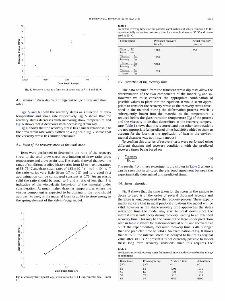
Fig. 6. Recovery stress as a function of strain rate at l ¼ 4 and 65 �C.

Table 1Predicted recovery times for the possible combinations of values compared to theexperimentally determined recovery time for a sample drawn at 55 �C and recov-ered at 65 �C.

Combination Predicted recoverytime (s)

Actual recoverytime (s)

hDraw

EDraw¼ h55

E551203 550

hRecovery

ERecovery¼ h65

E651291

hDraw

ERecovery¼ h55

E653884

hRecovery

EDraw¼ h65

E55524

M. Bonner et al. / Polymer 51 (2010) 1432–1436 1435

4.3. Transient stress dip tests at different temperatures and strainrates

Figs. 5 and 6 show the recovery stress as a function of drawtemperature and strain rate respectively. Fig. 5 shows that therecovery stress decreases with increasing draw temperature andFig. 6 shows that it decreases with decreasing strain rate.

Fig. 6 shows that the recovery stress has a linear relationship tothe draw strain rate when plotted on a log scale. Fig. 7 shows thatthe viscosity stress has similar behaviour.

4.4. Ratio of the recovery stress to the total stress

Tests were performed to determine the ratio of the recoverystress to the total draw stress as a function of draw ratio, drawtemperature and draw strain rate. The results showed that over therange of conditions studied (draw ratios from 1.5 to 4, temperaturesof 55–75 �C and draw strain rates of 1.33� 10�4 s�1 to 1�10�1 s�1)the ratio varies very little (from 0.7 to 0.8) and to a good firstapproximation can be considered constant at 0.75. For an elasticsolid the ratio should be equal to 1 and a ratio of less than 1 isindicative of the viscoelastic behaviour of the material underconsideration. At much higher drawing temperatures where theviscous component is expected to be dominant, the ratio shouldapproach to zero, as the material loses its ability to store energy inthe spring element of the Kelvin–Voigt model.

0

1

2

3

4

5

6

7

8

0.01 0.1 1

Vis

co

sity

S

tre

ss

(M

Pa

)

Draw Strain Rate (s-1

)

Fig. 7. Viscosity stress against log10 strain rate at 65 �C. (A experimental data, – linearfit).

4.5. Prediction of the recovery time

The data obtained from the transient stress dip tests allow thedetermination of the two components of the model ER and hR.However we must consider the appropriate combination ofpossible values to place into the equation. It would seem appro-priate to consider the recovery stress as the recovery stress devel-oped in the material during the deformation process, which issubsequently frozen into the material as the temperature isreduced below the glass transition temperature (Tg) of the processand the viscosity to be that determined at the recovery tempera-ture. Table 1 shows that this is correct and that other combinationsare not appropriate (all predicted times had 200 s added to them toaccount for the fact that the application of heat in the environ-mental chamber was not instantaneous).

To confirm this a series of recovery tests were performed usingdifferent drawing and recovery conditions, with the predictedrecovery times being based on

s ¼hRecovery

EDraw(6)

The results from these experiments are shown in Table 2 where itcan be seen that in all cases there is good agreement between theexperimentally determined and predicted times.

4.6. Stress relaxation

Fig. 8 shows that the time taken for the stress in the sample todecay to zero is of the order of several thousand seconds andtherefore is long compared to the recovery process. These experi-ments indicate that in most practical situations the model will bevalid, however as the shape recovery time approaches the stressrelaxation time the model may start to break down since theinternal stress will decay during recovery, leading to an extendedrecovery time. This may be the cause of the large under predictionseen in Table 2, where for material drawn at 65 �C and recovered at55 �C the experimentally measured recovery time is 416 s longerthan the predicted time of 3884 s. An examination of Fig. 8 showsthat at 55 �C the internal stress has decayed to half of its originalvalue after 3000 s. At present it is not currently possible to modelthese long term recovery situations since this requires the

Table 2Predicted and actual recovery times for material drawn and recovered under a rangeof conditions.

Draw temp(�C)

Recovery temp(�C)

Predicted time(s)

Actual time(s)

55 55 1203 103055 65 524 55055 75 216 21265 55 3884 4300

0

0.1

0.2

0.3

0.4

0.5

0.6

0.7

0.8

0.9

1

0 1000 2000 3000 4000 5000 6000 7000

Re

la

tiv

e S

tre

ss

Time (s)

55ºC

65ºC

75ºC

Fig. 8. Stress relaxation curves for material drawn at a nominal strain rate of8.33 � 10�3 s�1 to l ¼ 4 at the temperatures shown.

M. Bonner et al. / Polymer 51 (2010) 1432–14361436

determination of the viscosity term after stress relaxation, wherewe currently have no data.

5. Conclusions

A Kelvin–Voigt model combined with the Transient Stress DipTest provides a simple yet powerful technique for predicting theshape recovery time of shape memory polymers (SMP), givingexcellent agreement between prediction and experiment forrecovery times of less than 1000 s and reasonable agreement forrecovery times up to 4500 s. It was shown that shape recovery ofSMP occurs when the spring component of the Kelvin–Voigt modelor stored stress in the material exerts a force capable of deformingthe viscous component or the dashpot element of the model at thetemperature of shape recovery.

It was also found that the ratio of the recovery stress to the totalstress is to a good approximation invariant for the three processingvariables under consideration, namely drawing temperature, strainrate and draw ratio.

It is quite usual to describe the glassy stress–strain behaviour ofpolymers in terms of spring and dashpot elements. A commonfeature of such models involves a non-linear viscous dashpot,usually in series with a very stiff spring,in parallel with a weakerspring which provides strain hardening at high strains. The latter isoften modelled by a rubber-like network, most simply a Gaussiannetwork [12–16]. It is interesting that the spring element in thepresent investigation which relates to the internal stress, can alsobe described empirically by an affine deformation rubber elasticmodel although the deformation occurs in the glassy state below Tg.This result is consistent with the observations of Wendlandt et al.[17] who studied the development of segmental orientation inPMMA by NMR and showed that this followed the affine defor-mation model. The network structure for the number of Kuhnsegments was however much smaller than the entanglementnetwork found in the melt. Similar results were obtained by vanMelick et al. [18] for the strain hardening modulus of polystyreneblends where it was shown that this decreased with increasingtemperature as found in the present investigation.

It is not considered appropriate in this paper to pursuea detailed molecular interpretation of the results. Corrections to theapparent effective modulus of the recovery stress to take intoaccount the filler content of 35 wt% calcium carbonate(modulus35 Gpa [19]), using the method proposed by Chow [20], givecorrected effective moduli of 3.55 Mpa and 1.12 Mpa at 55 �C and65 �C respectively. Classical network theory, assuming appropriatemolecular weights for the monomer components of the polymer,then predicts 15 and 43 monomer units between the junctionpoints of the effective network at 55 �C and 65 �C respectively.

Following Fotheringham and Cherry [9] the viscosity stress canbe considered to be a thermally activated process. Most simply itcan be modelled by a single Eyring process with a strain ratedependence at high stress given by

_3 ¼ _30exp��

DU � sVkT

�(7)

i.e.,

ln _3 ¼ ln _30 �DUkTþ sV

kT(8)

Fig. 7 shows the experimental results at 65 �C from which a valuefor V of 5, 300 Å3 is obtained, similar to results for polymersreported by Haward and Thackray [12], Truss et al. [21] andFotheringham and Cherry [9] who did however consider it better toassume cooperative jumps of several chain segments and hencearrive at a smaller activation volume.

Acknowledgements

The authors wish to thank Yorkshire Forward and the Tech-nology Strategy Board for their financial support during this work.

References

[1] Liu C, Qin H, Mather PT. J Mater Chem 2007;17:1543–58.[2] Mather PT, Luo X, Rousseau IA. Annu Rev Mater Res 2009;39:445–71.[3] Sokolowsky W, Metcalfe A, Hayashi S, Yahia L, Raymond J. Biomed Mater

2007;2:S23–7.[4] Nguyen TD, Qi HJ, Castro F, Long KN. J Mech Phys Solids 2008;56:2792–814.[5] Chen YC, Lagoudas DC. J Mech Phys Solids 2008;56:1766–78.[6] Li F, Larock RC. J Appl Polym Sci 2002;84:1533–43.[7] Lin JR, Chen LW. J Polymer Res 1999;6:35–40.[8] Lin JR, Chen LW. J Appl Polym Sci 1999;73:1305–19.[9] Fotheringham DG, Cherry BW. J Mater Sci 1978;13:951–64.

[10] Ward IM. Mechanical properties of solid polymers. 2nd ed. Chichester: Wiley;1983.

[11] Treloar LRG. The physics of rubber elasticity. 3rd ed. Oxford: Clarendon Press;1975.

[12] Haward RN, Thackray G. Proc Roy Soc Lond A 1968;302:453.[13] Boyce MC, Parks DM, Argon A. Mech Mater 1988;7:15–33.[14] Arruda EM, Boyce MC. Int J Plast 1993;9:697–720.[15] Buckley CP, Jones DC. Polymer 1995;36:3301–12.[16] Tervoort TA, Smit RJM, Brekelmans WAM, Govaert LE. Time Dependent Mater

1997;1:269–91.[17] Wendlandt M, Tervoort TA, van Beck JD, Suter UW. J Mech Phys Solids

2006;54:599–610.[18] van Melick HGH, Govaert LE, Meijer HEH. Polymer 2003;44:2493–502.[19] Lutz JT, Grossman RF. Polymer modifiers and additives. CRC Press; 2000.[20] Chow TS. J Mater Sci 1980;15:1873–88.[21] Truss RW, Clarke PL, Duckett RA, Ward IM. J Polym Sci Polym Phys Ed

1984;22:191–209.