a new creep model directly using tabulated test data …

A new creep model directly using tabulated test data and implemented in ANSYS

XIV International Conference on Computational Plasticity. Fundamentals and Applications COMPLAS 2017

Kang Shen, Wilhelm J.H. Rust

A NEW CREEP MODEL DIRECTLY USING TABULATED TEST DATA AND IMPLEMENTED IN ANSYS

KANG SHEN, WILHELM J.H. RUST

Hochschule Hannover –University of Applied Sciences und Arts Faculty II department of Mechanical Engineering

Ricklinger Stadtweg 120 30459 Hannover, Germany E-mail: [email protected], [email protected]

Keywords: creep, material model, tabulated test data, ANSYS.

Abstract. Nowadays plastics are increasingly used in highly stressed structures in all kinds of constructions. The time dependency, the so-called viscosity, is a crucial part of the material behavior of plastics. A typical form of viscosity is creep. Creep is the increase of deformation under constant load. In the FE-simulation creep behavior is usually described by creep law functions. The commercial software provide many creep law functions depending on time, stress, strain, temperature and multiple material parameters. To run a creep simulation, the user must define all the parameters which requires a certain effort. Curve-fitting procedures might be of help, the results, however, often are not precise enough. For these reasons, we introduce our new creep model doing the similar job as the creep law functions but being able to directly use the tabulated data of the creep tests without curve-fitting procedures. In this paper, we use the model to create a 3D stress-creep strain-time surface based on the tabulated data like isoch-ronous curves, which is represented by bicubically blended Coons patches to provide a good convergence due to their differentiability. This creep model supports strain hardening, which shows more realistic behavior when the load changes significantly during the simulated process.

1 INTRODUCTION

Numerous plastics show a combined material behavior like elastic, plastic and viscous one. The viscosity of plastics strongly depends on the loading rate, the loading duration and the temperature [1, 2]. Ignoring the viscosity of plastics like creep can lead to a severe failure of construction based on simulation [3]. Creep describes the increase of the deformation with time under a mechanical stress [4].

The simulation of creep behavior is based on the creep test data. The creep is directly meas-ured from the creep and relaxation test. Creep curve provides a dependence of creep strain on time, relaxation curve provides a dependence of stress on time while creep strain can indirectly be determined. The isochronous curves are concluded from those two types of curve [5]. The isochronous curve gives a stress-strain relation at the identical time point.

Another well-established curve for creep is the creep modulus curve. The creep modulus is the quotient of the stress and total strain, thus showing a combination of creep and elastic be-havior over time. Considering Young’s modulus as constant there is a direct relation to creep strain.

319


2

Besides of stress and time creep behavior of plastics also depends on temperature. Conven-tional creep models usually describe the temperature dependency using the Arrhenius equation showing exponentially growing creep rates with respect to the inverse of the temperature [6]. Modelling temperature dependency in this way shows limited accuracy. On the other hand creep rate indeed varies nonlinearly with the temperature. Thus, the alternative, linearly interpolating all creep parameters might better match the material behavior for the given temperatures but lacks in between.

2 MOTIVATION Numerous creep models proposed creep law functions defining creep behavior. For those

functions several more or less abstract, not directly measurable material parameters must be specified. The difficulty is to determine the parameters as accurate for general application. Of-ten one creep curve for a single stress can be fitted accurately. The other dependencies, those of temperature and stress, then show larger errors if - which is often the case - the curves for different stress levels are not similar in the mathematical sense, i.e. not scalable. Furthermore, it has to be emphasized that usual creep models give functions not for creep strain but for strain rate. Curve fitting requires either the solution of the differential equation given in this way or the determination of strain rates from measured strain which can be difficult due to either a small number of sampling points or oscillations in the measured curves if the number of sam-pling points is larger. The study of [7] indicate that general curve fitting functions could create insufficiently accurate or even wrong parameters and mislead the simulation. As a consequence the user has a larger effort to determine creep parameters and will even though finally not be satisfied.

Furthermore, due to numeric (time integration scheme) creep rate models can be subject to larger initial errors, e.g. for the power function of time with negative exponent, even if the analytical use of the parameters show good accordance with tests. The latter is the reason why the authors avoid rate formulations but use incremental ones as shown below.

Despite the right selection of creep model and define its parameter, the material behavior of a creep model can also differ from the test data[8,9]. The reason for that is the fact that constant material parameters compromise the accuracy with multiple loads and temperatures. With the compromise the material behavior in simulation is only accurate in a limited range [10].

In this work, we focus our attention on the construction of a creep model with direct use of tabulated test data from the creep test. The tabulated data here are e.g. the creep-time curve, isochronous curve and creep modulus curve. This creep model works without parameter iden-tification and the curve fitting function. Instead of the parameters it uses a three-dimensional surface to find the proper creep state for calculation. For a good differentiability and a decent extensionality, we decided to use bicubical Coons patches (also named bicubically blended Coons patches) for the surface construction.

3 CONVENTIONAL CREEP MODEL Numerous conventional creep models describe the creep behavior using strain rate formu-

lation in a creep equation like: 𝜀𝜀̇𝑐𝑐𝑐𝑐 = 𝑓𝑓(𝜎𝜎, 𝑡𝑡, 𝜀𝜀, 𝑇𝑇) (1)

320


3

It shows that the creep strain rate depends on stress, time (or creep strain) and temperature. The dependencies of time and strain are normally not modelled within the same creep equation. As example, a creep equation of direct time dependency (also called time hardening) is defined as

𝜀𝜀̇𝑐𝑐𝑐𝑐 = 𝐶𝐶1𝜎𝜎𝑐𝑐2𝑡𝑡𝑐𝑐3 ⋅ 𝑒𝑒−𝑐𝑐4𝑇𝑇 (2)

whereas an example for indirect time dependency (strain-hardening), which show better accu-racy if the stress significantly changes (or creep process is interrupted) during the simulation, reads

𝜀𝜀̇𝑐𝑐𝑐𝑐 = 𝐶𝐶1𝜎𝜎𝑐𝑐2(𝜀𝜀𝑐𝑐𝑐𝑐)𝑐𝑐3 ⋅ 𝑒𝑒−𝑐𝑐4𝑇𝑇 (3)

where the 𝐶𝐶1 …𝐶𝐶4 are the material parameter. These parameters are fitted to the creep test data for a number of stress, time (or creep strain) and temperature points. The creep strain rate for a single curve may be accurate. However, the parameter identification goes easily wrong consid-ering multiple stress levels at different time point. The reason is that the stress, time and creep strain have a complex relation. Furthermore, defining the material parameter for indirect time dependency is harder than for the direct way, since the creep strain rate depends on the creep strain which makes the solution of the differential equation more difficult.

4 SURFACE CONSTRUCTION In our new creep model, we need a three-dimensional surface to describe the creep strain

depending on time and stress.1 The new creep model uses three types of creep test data for the users’ convenience. The creep test data can be the creep-time curve, isochronous curve and creep modulus curve.

The creep curve uses stress as curve parameter and describes the increase of creep strain with time. The isochronous curve connects stress-strain points at the same time level and is not a directly measured curve. These curves describe the strain-stress-time relation. Since the creep strain is our primary variable, the surface should be

𝜀𝜀𝑐𝑐𝑐𝑐 = 𝑓𝑓𝑐𝑐𝑐𝑐(𝜎𝜎, 𝑡𝑡) (4)

To create the surface with the given curves as tabulated data, we need to construct the curves in both 𝜎𝜎- and 𝑡𝑡-directions first. The curve requires to smoothly cross all the data points in one direction due to accuracy and differentiability. Thus, the cubic spline is used to create the curve. The advantage to build the cubic spline is that the spline exactly meets selected data points, avoid an unnecessary oscillation and provide 𝐶𝐶2-continuity. The spline for creep strain and time uses the logarithmic timeline due to rapid change of the creep strain at the beginning.

The surface is based on cubic splines as boundary curves. It should fit the splines and be smooth perpendicular to the edges. For this purpose, we use the bicubical Coons patches. The Coons patches use the boundary curves to generate surfaces [12, 13]. A bicubical Coons patch combines four edges from splines and the surface interpolation with the cubic Hermite Interpo-lation. We define the Hermite functions with cubical Bézier form as:

1The temperature effect is discussed in section 6.

321


4

𝐵𝐵03(𝜎𝜎) = (1 − 𝜎𝜎)3𝐵𝐵13(𝜎𝜎) = 3𝜎𝜎(1 − 𝜎𝜎)2𝐵𝐵23(𝜎𝜎) = 3𝜎𝜎2(1 − 𝜎𝜎)𝐵𝐵33(𝜎𝜎) = 𝜎𝜎3

(5)

So that Hermite function for 𝜎𝜎 ∈ [𝑎𝑎, 𝑏𝑏] is: 𝐻𝐻03(𝜎𝜎) = 𝐵𝐵03(𝜎𝜎) + 𝐵𝐵13(𝜎𝜎)𝐻𝐻13(𝜎𝜎) =

13 (𝑏𝑏 − 𝑎𝑎)𝐵𝐵1

3(𝜎𝜎)𝐻𝐻23(𝜎𝜎) = −

13 (𝑏𝑏 − 𝑎𝑎)𝐵𝐵2

3(𝜎𝜎)𝐻𝐻33(𝜎𝜎) = 𝐵𝐵23(𝜎𝜎) + 𝐵𝐵33(𝜎𝜎)

(6)

From the cubical spline, the positional data is available for Coons patch, the four splines are: 𝑓𝑓(𝑎𝑎, 𝑡𝑡), 𝑓𝑓(𝑏𝑏, 𝑡𝑡), 𝑓𝑓(𝜎𝜎, 𝑐𝑐), 𝑓𝑓(𝜎𝜎, 𝑑𝑑) (7)

which 𝜎𝜎 ∈ [𝑎𝑎, 𝑏𝑏], 𝑡𝑡 ∈ [𝑐𝑐, 𝑑𝑑]. For purpose of continuity, first derivative information for both 𝜎𝜎- and t-direction is desired but not given. The two patches, which share the same edge in 𝜎𝜎- or t-direction, must have the same derivative in t- resp. 𝜎𝜎-direction of the edge. Therefore, the de-rivative is defined through a linear interpolation from two ends of the edge. Hence, there are four derivatives for each boundary:

𝜕𝜕𝑓𝑓(𝑎𝑎, 𝑡𝑡)𝜕𝜕𝜎𝜎 , 𝜕𝜕𝑓𝑓

(𝑏𝑏, 𝑡𝑡)𝜕𝜕𝜎𝜎 , 𝜕𝜕𝑓𝑓

(𝜎𝜎, 𝑐𝑐)𝜕𝜕𝑡𝑡 , 𝜕𝜕𝑓𝑓

(𝜎𝜎, 𝑑𝑑)𝜕𝜕𝑡𝑡

(8)

Through four boundary curves and their derivatives two ruled surfaces are defined: ℎ𝑐𝑐(𝜎𝜎, 𝑡𝑡) = 𝐻𝐻03(𝜎𝜎) ⋅ 𝑓𝑓(𝑎𝑎, 𝑡𝑡) + 𝐻𝐻13(𝜎𝜎) ⋅

𝜕𝜕𝑓𝑓(𝑎𝑎, 𝑡𝑡)𝜕𝜕𝜎𝜎 + 𝐻𝐻23(𝜎𝜎) ⋅

𝜕𝜕𝑓𝑓(𝑏𝑏, 𝑡𝑡)𝜕𝜕𝜎𝜎 + 𝐻𝐻33(𝜎𝜎) ⋅ 𝑓𝑓(𝑏𝑏, 𝑡𝑡)

ℎ𝑑𝑑(𝜎𝜎, 𝑡𝑡) = 𝐻𝐻03(𝑡𝑡) ⋅ 𝑓𝑓(𝜎𝜎, 𝑐𝑐) + 𝐻𝐻13(𝑡𝑡) ⋅𝜕𝜕𝑓𝑓(𝜎𝜎, 𝑐𝑐)𝜕𝜕𝑡𝑡 + 𝐻𝐻23(𝑦𝑦) ⋅

𝜕𝜕𝑓𝑓(𝜎𝜎, 𝑑𝑑)𝜕𝜕𝑡𝑡 + 𝐻𝐻33(𝑡𝑡) ⋅ 𝑓𝑓(𝜎𝜎, 𝑑𝑑)

(9)

The interpolated surface ℎ𝑐𝑐(𝜎𝜎, 𝑡𝑡) is ruled by the splines 𝑓𝑓(𝑎𝑎, 𝑡𝑡), 𝑓𝑓(𝑏𝑏, 𝑡𝑡) in t-direction for 𝜎𝜎 ∈[𝑎𝑎, 𝑏𝑏] and ℎ𝑑𝑑(𝜎𝜎, 𝑡𝑡) is ruled by the splines 𝑓𝑓(𝜎𝜎, 𝑐𝑐), 𝑓𝑓(𝜎𝜎, 𝑑𝑑) in 𝜎𝜎-direction for 𝑡𝑡 ∈ [𝑐𝑐, 𝑑𝑑].Thus, we need ℎ𝑐𝑐(𝜎𝜎, 𝑡𝑡) to fix its course in t-direction and change its course in 𝜎𝜎-direction like ℎ𝑑𝑑(𝜎𝜎, 𝑡𝑡). In this case, a new surface is used to achieve this goal. We define a surface with the corner data for the interpolation:

ℎ𝑐𝑐𝑑𝑑(𝜎𝜎, 𝑡𝑡) = (𝐻𝐻03(𝜎𝜎) 𝐻𝐻13(𝜎𝜎)𝐻𝐻23(𝜎𝜎) 𝐻𝐻33(𝜎𝜎)) ⋅

(

𝑓𝑓(𝑎𝑎, 𝑐𝑐) 𝜕𝜕𝑓𝑓(𝑎𝑎, 𝑐𝑐)

𝜕𝜕𝑡𝑡𝜕𝜕𝑓𝑓(𝑎𝑎, 𝑐𝑐)𝜕𝜕𝜎𝜎 0

𝜕𝜕𝑓𝑓(𝑎𝑎, 𝑑𝑑)𝜕𝜕𝑡𝑡 𝑓𝑓(𝑎𝑎, 𝑑𝑑)

0 𝜕𝜕𝑓𝑓(𝑎𝑎, 𝑑𝑑)𝜕𝜕𝜎𝜎

𝜕𝜕𝑓𝑓(𝑏𝑏, 𝑐𝑐)𝜕𝜕𝜎𝜎 0

𝑓𝑓(𝑏𝑏, 𝑐𝑐) 𝜕𝜕𝑓𝑓(𝑏𝑏, 𝑐𝑐)𝜕𝜕𝑡𝑡

0 𝜕𝜕𝑓𝑓(𝑏𝑏, 𝑑𝑑)𝜕𝜕𝜎𝜎

𝜕𝜕𝑓𝑓(𝑏𝑏, 𝑑𝑑)𝜕𝜕𝑡𝑡 𝑓𝑓(𝑏𝑏, 𝑑𝑑) )

⋅

(

𝐻𝐻03(𝑡𝑡)𝐻𝐻13(𝑡𝑡)𝐻𝐻23(𝑡𝑡)𝐻𝐻33(𝑡𝑡))

(10)

The bicubical Coons Patch is defined as: ℎ𝑔𝑔(𝜎𝜎, 𝑡𝑡) = ℎ𝑐𝑐(𝜎𝜎, 𝑡𝑡) + ℎ𝑑𝑑(𝜎𝜎, 𝑡𝑡) − ℎ𝑐𝑐𝑑𝑑(𝜎𝜎, 𝑡𝑡) (11)

322


5

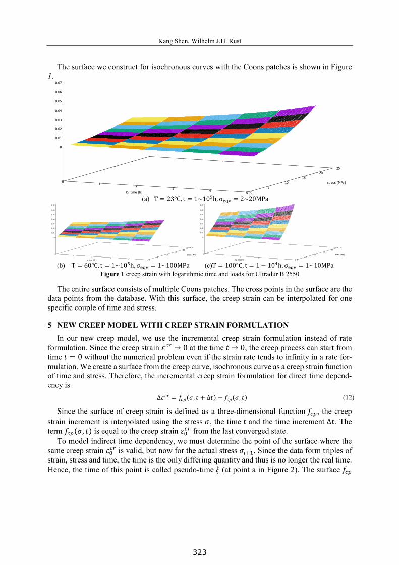
The surface we construct for isochronous curves with the Coons patches is shown in Figure 1.

(a) T = 23°C, t = 1~105h, σeqv = 2~20MPa

(b) T = 60°C, t = 1~105h, σeqv = 1~100MPa (c)T = 100°C, t = 1 − 104h, σeqv = 1~10MPa

Figure 1 creep strain with logarithmic time and loads for Ultradur B 2550

The entire surface consists of multiple Coons patches. The cross points in the surface are the data points from the database. With this surface, the creep strain can be interpolated for one specific couple of time and stress.

5 NEW CREEP MODEL WITH CREEP STRAIN FORMULATION In our new creep model, we use the incremental creep strain formulation instead of rate

formulation. Since the creep strain 𝜀𝜀𝑐𝑐𝑐𝑐 → 0 at the time 𝑡𝑡 → 0, the creep process can start from time 𝑡𝑡 = 0 without the numerical problem even if the strain rate tends to infinity in a rate for-mulation. We create a surface from the creep curve, isochronous curve as a creep strain function of time and stress. Therefore, the incremental creep strain formulation for direct time depend-ency is

Δ𝜀𝜀𝑐𝑐𝑐𝑐 = 𝑓𝑓𝑐𝑐𝑐𝑐(𝜎𝜎, 𝑡𝑡 + Δ𝑡𝑡) − 𝑓𝑓𝑐𝑐𝑐𝑐(𝜎𝜎, 𝑡𝑡) (12)

Since the surface of creep strain is defined as a three-dimensional function 𝑓𝑓𝑐𝑐𝑐𝑐, the creep strain increment is interpolated using the stress 𝜎𝜎, the time 𝑡𝑡 and the time increment Δ𝑡𝑡. The term 𝑓𝑓𝑐𝑐𝑐𝑐(𝜎𝜎, 𝑡𝑡) is equal to the creep strain 𝜀𝜀0𝑐𝑐𝑐𝑐 from the last converged state.

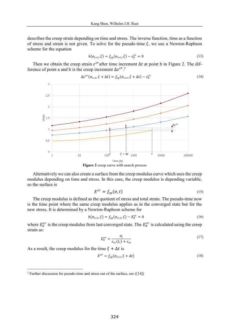
To model indirect time dependency, we must determine the point of the surface where the same creep strain 𝜀𝜀0𝑐𝑐𝑐𝑐 is valid, but now for the actual stress 𝜎𝜎𝑖𝑖+1. Since the data form triples of strain, stress and time, the time is the only differing quantity and thus is no longer the real time. Hence, the time of this point is called pseudo-time 𝜉𝜉 (at point a in Figure 2). The surface 𝑓𝑓𝑐𝑐𝑐𝑐

0 1

2 3

4 5 0 5

10 15

20 25

0

0.01

0.02

0.03

0.04

0.05

0.06

0.07

cree

p st

rain

lg. time [h]

stress [MPa]

cree

p st

rain

0 1

2 3

4 5 0 5

10 15

20 25

0

0.01

0.02

0.03

0.04

0.05

0.06

0.07

cree

p st

rain

lg. time [h]

stress [MPa]

cree

p st

rain

0 1

2 3

4 5 0 5

10 15

20 25

0

0.01

0.02

0.03

0.04

0.05

0.06

0.07

cree

p st

rain

lg. time [h]

stress [MPa]

cree

p st

rain

323


6

describes the creep strain depending on time and stress. The inverse function, time as a function of stress and strain is not given. To solve for the pseudo-time 𝜉𝜉, we use a Newton-Raphson scheme for the equation

ℎ(𝜎𝜎𝑖𝑖+1, 𝜉𝜉) = 𝑓𝑓𝑐𝑐𝑐𝑐(𝜎𝜎𝑖𝑖+1, 𝜉𝜉) − 𝜀𝜀0𝑐𝑐𝑐𝑐 = 0 (13)

Then we obtain the creep strain 𝜀𝜀𝑐𝑐𝑐𝑐after time increment Δ𝑡𝑡 at point b in Figure 2. The dif-ference of point a and b is the creep increment Δ𝜀𝜀𝑐𝑐𝑐𝑐.2

Δ𝜀𝜀𝑐𝑐𝑐𝑐(𝜎𝜎𝑖𝑖+1, 𝜉𝜉 + Δ𝑡𝑡) = 𝑓𝑓𝑐𝑐𝑐𝑐(𝜎𝜎𝑖𝑖+1, 𝜉𝜉 + Δ𝑡𝑡) − 𝜀𝜀0𝑐𝑐𝑐𝑐 (14)

Figure 2 creep curve with search process

Alternatively we can also create a surface from the creep modulus curve which uses the creep modulus depending on time and stress. In this case, the creep modulus is depending variable, so the surface is

𝐸𝐸𝑐𝑐𝑐𝑐 = 𝑓𝑓𝑐𝑐𝑐𝑐(𝜎𝜎, 𝑡𝑡) (15)

The creep modulus is defined as the quotient of stress and total strain. The pseudo-time now is the time point where the same creep modulus applies as in the converged state but for the new stress. It is determined by a Newton-Raphson scheme for

ℎ(𝜎𝜎𝑖𝑖+1, 𝜉𝜉) = 𝑓𝑓𝑐𝑐𝑐𝑐(𝜎𝜎𝑖𝑖+1, 𝜉𝜉) − 𝐸𝐸0𝑐𝑐𝑐𝑐 = 0 (16)

where 𝐸𝐸0𝑐𝑐𝑐𝑐 is the creep modulus from last converged state. The 𝐸𝐸0𝑐𝑐𝑐𝑐 is calculated using the creep strain as:

𝐸𝐸0𝑐𝑐𝑐𝑐 =𝜎𝜎𝑖𝑖

𝜀𝜀𝑐𝑐𝑐𝑐(𝑡𝑡𝑖𝑖) + 𝜀𝜀𝑒𝑒𝑒𝑒 (17)

As a result, the creep modulus for the time 𝜉𝜉 + Δ𝑡𝑡 is 𝐸𝐸𝑐𝑐𝑐𝑐 = 𝑓𝑓𝑐𝑐𝑐𝑐(𝜎𝜎𝑖𝑖+1, 𝜉𝜉 + Δ𝑡𝑡) (18)

2 Further discussion for pseudo-time and stress out of the surface, see ([14])

324


7

To use the same local iteration of creep strain formulation (Figure 3), we convert creep modulus to creep strain

∆𝜀𝜀𝑐𝑐𝑐𝑐(𝜎𝜎𝑖𝑖+1, 𝑡𝑡 + Δ𝑡𝑡) = 𝜎𝜎𝑖𝑖+1𝐸𝐸𝑐𝑐𝑐𝑐(𝜎𝜎𝑖𝑖+1, 𝜉𝜉 + Δ𝑡𝑡) −

𝜎𝜎𝑖𝑖+1𝐸𝐸 − 𝜀𝜀0𝑐𝑐𝑐𝑐 (19)

where the first term is the new total strain and the second one the new elastic strain. Its partial derivative with respect to 𝜎𝜎 is

𝜕𝜕∆𝜀𝜀𝑐𝑐𝑐𝑐(𝜎𝜎𝑖𝑖+1, 𝑡𝑡 + Δ𝑡𝑡)𝜕𝜕𝜎𝜎 = 𝜕𝜕

𝜕𝜕𝜎𝜎 (𝜎𝜎𝑖𝑖+1

𝐸𝐸𝑐𝑐𝑐𝑐(𝜎𝜎𝑖𝑖+1, 𝜉𝜉 + Δ𝑡𝑡)) −1𝐸𝐸 = 1

𝐸𝐸𝑐𝑐𝑐𝑐− 𝜎𝜎𝐸𝐸𝑐𝑐𝑐𝑐2

𝜕𝜕𝐸𝐸𝑐𝑐𝑐𝑐𝜕𝜕𝜎𝜎 − 1

𝐸𝐸 (20)

and with respect to 𝑡𝑡 : 𝜕𝜕∆𝜀𝜀𝑐𝑐𝑐𝑐(𝜎𝜎𝑒𝑒𝑒𝑒𝑒𝑒,𝑖𝑖+1, 𝑡𝑡 + Δ𝑡𝑡)

𝜕𝜕𝑡𝑡 = − 𝜎𝜎𝐸𝐸𝑐𝑐𝑐𝑐2

𝜕𝜕𝐸𝐸𝑐𝑐𝑐𝑐𝜕𝜕𝑡𝑡

(21)

Thus, all three types of test data curves are united by the incremental creep strain formulation. With the creep strain increment, the three-dimensional creep state is defined

Δ𝜺𝜺𝑐𝑐𝑐𝑐 = Δ𝜀𝜀𝑐𝑐𝑐𝑐 ⋅ 𝜕𝜕𝜕𝜕𝜕𝜕𝝈𝝈 (22)

where 𝜕𝜕 is plastic potential. This equation is adopted from the flow rule of plastic material, where the plastic multiplier is replaced by the creep strain increment in this case. Like in plas-tics, we use the flow rule associated with the yield condition 𝐹𝐹 after von Mises. There is no threshold like the yield stress, thus creep is always present if there is non-zero equivalent stress.

After the Δ𝜺𝜺𝑐𝑐𝑐𝑐 is determined, the current stress state is

𝝈𝝈 = 𝑬𝑬 (𝜺𝜺𝑡𝑡𝑡𝑡𝑡𝑡 − 𝜺𝜺𝑐𝑐𝑐𝑐(ti) − Δ𝜺𝜺𝑐𝑐𝑐𝑐(𝜉𝜉 + Δ𝑡𝑡, 𝜎𝜎𝑒𝑒𝑒𝑒𝑒𝑒(𝝈𝝈))) (23)

where 𝑬𝑬 is the elasticity matrix, 𝜺𝜺𝑡𝑡𝑡𝑡𝑡𝑡 is total strain for this step. The stress state changes with the creep increment updates. The equivalent stress is defined after von Mises. In equation (23), stress tensor 𝝈𝝈 is defined implicitly. Therefore, a local iteration with Newton-Raphson method should take place

𝑔𝑔 = Δ𝜀𝜀𝑐𝑐𝑐𝑐 − Δ𝜀𝜀𝑐𝑐𝑐𝑐(𝜎𝜎𝑒𝑒𝑒𝑒𝑒𝑒(𝝈𝝈), 𝜉𝜉 + Δ𝑡𝑡) − 𝜀𝜀𝑒𝑒𝑒𝑒𝑒𝑒𝑐𝑐𝑐𝑐 (𝑡𝑡𝑖𝑖) = 0 (24)

The derivative of 𝑔𝑔 is 𝜕𝜕𝑔𝑔

𝜕𝜕Δ𝜀𝜀𝑐𝑐𝑐𝑐 = 1 + 𝜕𝜕Δ𝜀𝜀𝑐𝑐𝑐𝑐𝜕𝜕𝜎𝜎𝑒𝑒𝑒𝑒𝑒𝑒

(𝜕𝜕𝜕𝜕𝜕𝜕𝝈𝝈)𝑇𝑇𝑬𝑬𝜕𝜕𝜕𝜕𝜕𝜕𝝈𝝈 − 𝜕𝜕Δ𝜀𝜀𝑐𝑐𝑐𝑐

𝜕𝜕𝜀𝜀𝑐𝑐𝑐𝑐 (25)

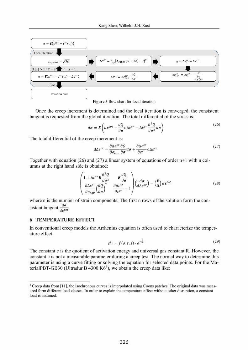
For each iteration, the creep increment and its derivative is determined using the surface of Coons patches. The process for the creep increment calculation is shown in Figure 3

325


8

Figure 3 flow chart for local iteration

Once the creep increment is determined and the local iteration is converged, the consistent tangent is requested from the global iteration. The total differential of the stress is:

𝑑𝑑𝝈𝝈 = 𝑬𝑬(𝑑𝑑𝜺𝜺𝑡𝑡𝑡𝑡𝑡𝑡 − 𝜕𝜕𝜕𝜕𝜕𝜕𝝈𝝈 dΔ𝜀𝜀𝑐𝑐𝑐𝑐 − Δ𝜀𝜀𝑐𝑐𝑐𝑐 𝜕𝜕

2𝜕𝜕𝜕𝜕𝝈𝝈2 𝑑𝑑𝝈𝝈)

(26)

The total differential of the creep increment is:

dΔ𝜀𝜀𝑐𝑐𝑐𝑐 = 𝜕𝜕Δ𝜀𝜀𝑐𝑐𝑐𝑐

𝜕𝜕𝜎𝜎𝑒𝑒𝑒𝑒𝑒𝑒𝜕𝜕𝜕𝜕𝜕𝜕𝝈𝝈 𝑑𝑑𝝈𝝈 +

𝜕𝜕Δ𝜀𝜀𝑐𝑐𝑐𝑐𝜕𝜕𝜀𝜀𝑐𝑐𝑐𝑐 dΔ𝜀𝜀

𝑐𝑐𝑐𝑐 (27)

Together with equation (26) and (27) a linear system of equations of order n+1 with n col-umns at the right hand side is obtained:

(

𝟏𝟏 + Δ𝜀𝜀

𝑐𝑐𝑐𝑐𝑬𝑬 𝜕𝜕2𝜕𝜕𝜕𝜕𝝈𝝈2 𝑬𝑬 𝜕𝜕𝜕𝜕𝜕𝜕𝝈𝝈

𝜕𝜕Δ𝜀𝜀𝑐𝑐𝑐𝑐𝜕𝜕𝜎𝜎𝑒𝑒𝑒𝑒𝑒𝑒

(𝜕𝜕𝜕𝜕𝜕𝜕𝝈𝝈)𝑇𝑇 𝜕𝜕Δ𝜀𝜀𝑐𝑐𝑐𝑐

𝜕𝜕𝜀𝜀𝑐𝑐𝑐𝑐 + 1)

( 𝑑𝑑𝝈𝝈dΔ𝜀𝜀𝑐𝑐𝑐𝑐) = (

𝑬𝑬0)𝑑𝑑𝜺𝜺

𝑡𝑡𝑡𝑡𝑡𝑡 (28)

where n is the number of strain components. The first n rows of the solution form the con-sistent tangent 𝑑𝑑𝝈𝝈𝑑𝑑𝜺𝜺𝑡𝑡𝑡𝑡𝑡𝑡.

6 TEMPERATURE EFFECT In conventional creep models the Arrhenius equation is often used to characterize the temper-ature effect.

𝜀𝜀𝑐𝑐𝑐𝑐̇ = 𝑓𝑓(𝜎𝜎, 𝑡𝑡, 𝜀𝜀) ⋅ 𝑒𝑒−𝑐𝑐𝑇𝑇 (29)

The constant c is the quotient of activation energy and universal gas constant R. However, the constant c is not a measurable parameter during a creep test. The normal way to determine this parameter is using a curve fitting or solving the equation for selected data points. For the Ma-terialPBT-GB30 (Ultradur B 4300 K63), we obtain the creep data like:

3 Creep data from [11], the isochronous curves is interpolated using Coons patches. The original data was meas-ured form different load classes. In order to explain the temperature effect without other disruption, a constant load is assumed.

326


9

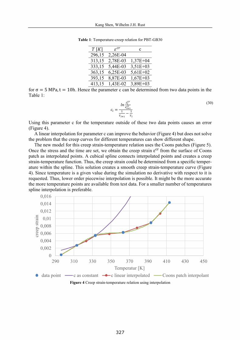
Table 1: Temperature-creep relation for PBT-GB30

𝑇𝑇 [𝐾𝐾] 𝜀𝜀𝑐𝑐𝑐𝑐 c 296,15 2,26E-04 313,15 2,78E-03 1,37E+04 333,15 5,44E-03 3,51E+03 363,15 6,25E-03 5,61E+02 393,15 8,87E-03 1,67E+03 413,15 1,43E-02 3,89E+03

for σ = 5 MPa, t = 10h. Hence the parameter c can be determined from two data points in the Table 1:

𝑐𝑐𝑖𝑖 =𝑙𝑙𝑙𝑙 �̇�𝜀𝑖𝑖

𝑐𝑐𝑐𝑐

�̇�𝜀𝑖𝑖+1𝑐𝑐𝑐𝑐

1𝑇𝑇𝑖𝑖+1

− 1𝑇𝑇𝑖𝑖

(30)

Using this parameter c for the temperature outside of these two data points causes an error (Figure 4).

A linear interpolation for parameter c can improve the behavior (Figure 4) but does not solve the problem that the creep curves for different temperatures can show different shape.

The new model for this creep strain-temperature relation uses the Coons patches (Figure 5). Once the stress and the time are set, we obtain the creep strain εcr from the surface of Coons patch as interpolated points. A cubical spline connects interpolated points and creates a creep strain-temperature function. Thus, the creep strain could be determined from a specific temper-ature within the spline. This solution creates a smooth creep strain-temperature curve (Figure 4). Since temperature is a given value during the simulation no derivative with respect to it is requested. Thus, lower order piecewise interpolation is possible. It might be the more accurate the more temperature points are available from test data. For a smaller number of temperatures spline interpolation is preferable.

Figure 4 Creep strain-temperature relation using interpolation

00,0020,0040,0060,0080,01

0,0120,0140,016

290 310 330 350 370 390 410 430 450

cree

p st

rain

Temperatur [K]data point c as constant c linear interpolated Coons patch interpolant

327


10

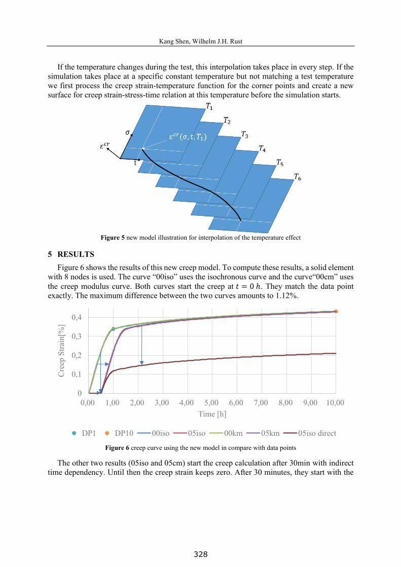
If the temperature changes during the test, this interpolation takes place in every step. If the simulation takes place at a specific constant temperature but not matching a test temperature we first process the creep strain-temperature function for the corner points and create a new surface for creep strain-stress-time relation at this temperature before the simulation starts.

Figure 5 new model illustration for interpolation of the temperature effect

5 RESULTS Figure 6 shows the results of this new creep model. To compute these results, a solid element

with 8 nodes is used. The curve “00iso” uses the isochronous curve and the curve“00cm” uses the creep modulus curve. Both curves start the creep at 𝑡𝑡 = 0 ℎ. They match the data point exactly. The maximum difference between the two curves amounts to 1.12%.

Figure 6 creep curve using the new model in compare with data points

The other two results (05iso and 05cm) start the creep calculation after 30min with indirect time dependency. Until then the creep strain keeps zero. After 30 minutes, they start with the

0

0,1

0,2

0,3

0,4

0,00 1,00 2,00 3,00 4,00 5,00 6,00 7,00 8,00 9,00 10,00

Cre

ep S

train

[%]

Time [h]

DP1 DP10 00iso 05iso 00km 05km 05iso direct

328


11

same curve as“00iso” and “00cm”. This result shows that the indirect time dependency work properly. For the direct time dependency the curve “05iso direct” is considering the creep pro-cess as already done for 30 minutes, so it starts with the range of the curve “00iso” beginning at the same time point. Thus, this creep model works as it should be.

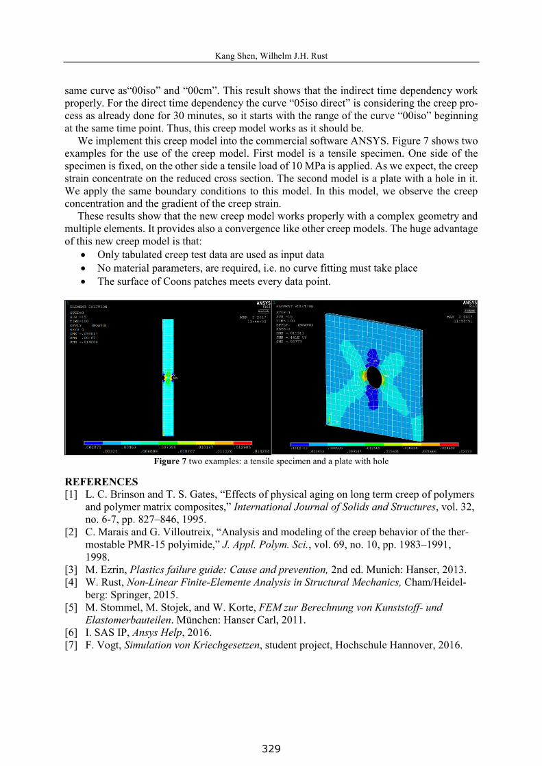
We implement this creep model into the commercial software ANSYS. Figure 7 shows two examples for the use of the creep model. First model is a tensile specimen. One side of the specimen is fixed, on the other side a tensile load of 10 MPa is applied. As we expect, the creep strain concentrate on the reduced cross section. The second model is a plate with a hole in it. We apply the same boundary conditions to this model. In this model, we observe the creep concentration and the gradient of the creep strain.

These results show that the new creep model works properly with a complex geometry and multiple elements. It provides also a convergence like other creep models. The huge advantage of this new creep model is that:

Only tabulated creep test data are used as input data No material parameters, are required, i.e. no curve fitting must take place The surface of Coons patches meets every data point.

Figure 7 two examples: a tensile specimen and a plate with hole

REFERENCES [1] L. C. Brinson and T. S. Gates, “Effects of physical aging on long term creep of polymers

and polymer matrix composites,” International Journal of Solids and Structures, vol. 32, no. 6-7, pp. 827–846, 1995.

[2] C. Marais and G. Villoutreix, “Analysis and modeling of the creep behavior of the ther-mostable PMR-15 polyimide,” J. Appl. Polym. Sci., vol. 69, no. 10, pp. 1983–1991, 1998.

[3] M. Ezrin, Plastics failure guide: Cause and prevention, 2nd ed. Munich: Hanser, 2013. [4] W. Rust, Non-Linear Finite-Elemente Analysis in Structural Mechanics, Cham/Heidel-

berg: Springer, 2015. [5] M. Stommel, M. Stojek, and W. Korte, FEM zur Berechnung von Kunststoff- und

Elastomerbauteilen. München: Hanser Carl, 2011. [6] I. SAS IP, Ansys Help, 2016. [7] F. Vogt, Simulation von Kriechgesetzen, student project, Hochschule Hannover, 2016.

329


12

[8] M. J. Dropik, D. H. Johnson, and D. E. Roth, “Developing an ANSYS creep model for polypropylene from experimental data,” in Proceedings of International ANSYS Confer-ence, 2002.

[9] Y. S. Kim and D. R. Metzger, “A finite element study of friction effect in four-point bending creep test,” in ASME 2003 Pressure Vessels and Piping Conference, 2003, pp. 99–107.

[10] T. Pulngern et al., “Effect of temperature on mechanical properties and creep responses for wood/PVC composites,” Construction and Building Materials, vol. 111, pp. 191–198, 2016.

[11] M-Base Engineering + Software GmbH, CAMPUS® Plastics Material Database. [Online] Available: http://www.campusplastics.com/campus/.

[12] G. Farin, Curves and surfaces for CAGD: A practical guide, 5th ed. San Francisco, Ca-lif.: Morgan Kaufmann Publ, 2006.

[13] S. A. Coons, “Surfaces for computer-aided design of space forms,” DTIC Document, 1967.

[14] Wilhelm J.H. Rust, Kang Shen, “Ein Kriechmodell für ANSYS unter direkter Verwen-dung von Versuchsdaten”,Proceedings of 34. CADFEM ANSYS Simulation Conference, 2016.

330

a new creep model directly using tabulated test data …

Documents