a new approach to forecasting exchange rates · a new approach to forecasting exchange rates+ by...
TRANSCRIPT
A NEW APPROACH TO
FORECASTING EXCHANGE RATES+
by
Kenneth W Clements and Yihui Lan∗
Business School The University of Western Australia
Abstract
Building on purchasing power parity theory, this paper proposes a new approach to forecasting exchange rates using the Big Mac data from The Economist magazine. Our approach is attractive in three aspects. Firstly, it uses easily-available Big Mac prices as input. These prices avoid several serious problems associated with broad price indexes, such as the CPI, that are used in conventional PPP studies. Secondly, this approach provides real-time exchange-rate forecasts at any forecast horizon. Such real-time forecasts can be made on a day-to-day basis if required, so that the forecasts are based on the most up-to-date information set. These high-frequency forecasts could be particularly appealing to decision makers who want up-to-date forecasts of exchange rates. Finally, as our forecasts are obtained through Monte Carlo simulation, estimation uncertainty is made explicit in our framework which provides the entire distribution of exchange rates, not just a single point estimate. A comparison of our forecasts with the random walk model shows that although the random walk is superior for very short horizons, our approach tends to dominate over the medium to longer term.
Keywords: Exchange-rate forecasting, Big Mac prices, purchasing power parity, Monte Carlo simulation
JEL Classification Code: F30, C53
+ This research was supported in part by the ARC, ACIL Tasman, AngloGold Ashanti and the WA Department of Industry and Resources. The views expressed herein are not necessarily those of the supporting bodies. We would like to thank the helpful comments of H. Y. Izan and of the participants in the Conference on “The Economics of Commodity Prices and Exchange Rates”, Perth, Australia, June 2006 and at the UWA FACTS Study Group seminar. ∗ Corresponding author. Phone: 61-8-6488-2464, Fax: 61-8-6488-1047, Email: [email protected].
1
“Most people dealing in the foreign exchange market have no clue about the fundamental value of the dollar (the “quality” of the dollar). Specialists and professors do not know either, at least within a broad range of dollar-euro rates between say, $1.0 and $1.3. For every specialist telling us that the fundamental value of the dollar is close to $1.3 to the euro there will be another one affirming that $1.0 is near the fundamental value. Anything in between is a fair game.”
Paul de Grauwe, Financial Times. Jan 13, 2006. p. 19.
1. Introduction
Since the breakdown of the Bretton Woods system of fixed exchange rates in the early
1970s, forecasting currency values has become crucial for many purposes such as international
comparisons of incomes, earnings and the costs of living by international agencies, management
and alignment of exchange rates by governments, and corporate financial decision making. Even
though it is widely agreed that forecasting exchange rates is a notoriously difficult task (as
indicated by de Grauwe’s comments above), there are still many attempts to do so. This paper
builds on purchasing power parity theory and introduces a new approach to forecast exchange
rates based on the Big Mac data published by The Economist magazine.
In the exchange-rate forecasting literature, the paper by Meese and Rogoff (1983) remains highly
influential as it demonstrates that structural models are unable to outperform the random walk
model, which simply predicts that the exchange rate would not change at all. Though the random
walk model has occupied center stage for many years, practitioners and researchers continue to
employ a variety of techniques in an effort to beat the random walk. Generally speaking, there are
three distinct approaches to exchange-rate forecasting:
• Surveys, which are popular among practitioners. But it is found that while survey forecasts
provide some predictive power (Lai, 1990, Chinn and Frankel, 1994a), sometimes they are
biased (Chinn and Frankel, 1994b) and unreliable (Harrison and Mogford, 2004).
• Model-based approaches, which include (i) fundamentals models, (ii) linear time series
models and (iii) non-linear time series models. The monetary approach is a popular
fundamentals model, with explanatory variables including relative prices levels, interest rate
differentials, and other determinants of equilibrium in the money market. Abhyabkara et al.
(2005) show that the economic value, as opposed to the statistical accuracy, of exchange-rate
forecasts based on a fundamentals model, can be greater than that based on the random walk
model. The traditionally-used linear time series models are the random walk, ARIMA, or
multivariate systems models such as the VAR model and the VECM. A recent stream of
research focuses on non-linear time series models, which includes the simultaneous nearest-
2
neighbour approach by Fernandez-Rodriguez et al. (1999), and the neural networks of Zhang
and Hu (1998).
• The composite forecast approach, which involves taking weighted averages of forecasts
from alternative approaches. MacDonald and Marsh (1994) review the earlier literature and
their examination of various methods of forecast combination shows that they can lead to
improvements in forecast accuracy. More recent examples of composite forecasts include Qi
and Wu (2003) in which neural networks and monetary fundamentals are used to model
exchange rates, and Alvarez-Diaz and Alvarez (2005) who combine forecasts from two non-
linear models.
PPP-based exchange-rate forecasts belong to the fundamentals stream of the model-based
approach, and use the relative price levels in two countries in question as fundamentals. There are
three versions of PPP: the absolute version, the relative version, and the stochastic relative version.
While the first two versions are often explained in textbooks, it is the third version that of
particular interest to researchers. Relative PPP implies that the exchange rate and the relative
prices are exactly proportional, so that the real exchange rate (the exchange rate deflated by
relative prices) is a constant. Stochastic relative PPP, on the other hand, allows for systematic
deviations from this constant, and treats this constant as the center of gravity to which the real
exchange rate reverts in the long run. Research on this weaker version of PPP examines the time-
series properties of exchange rates, and tests for mean reversion and the speed of adjustment to
long-run equilibrium values. The estimated long-run exchange rates and the speed-of-adjustment
parameters are then used for the purpose of exchange-rate forecasting.
In most studies of PPP, the real exchange rate is usually defined using the price index based on a
broad basket of goods, such as the consumer price index, wholesale price index, or GDP deflator.1
The use of broad indexes is subject to several serious problems however. First, many price
indexes are published only at infrequent intervals; in Australia, for example, the CPI is published
only quarterly and then with a considerable lag, which limits its usefulness for timely forecasts.
Second, differences in consumption patterns in different countries mean that broad indexes relate
to the prices of baskets of goods and services that can differ substantially internationally.2 In PPP
theory the ratio of prices at home to those abroad is meant to reflect differing monetary conditions
only, but when broad indexes are used, this ratio could be dominated by heterogeneity of 1 For an analysis of the impact of using differing broad price indexes on exchange-rate forecasts, see Xu (2003). 2 For example, food occupies less than 10 percent of total consumption in rich countries, while it absorbs something like 50 percent in the poorest.
3
consumption patterns. Thus, rather than comparing like with like to isolate the underlying
monetary factors, the CPI-based price ratios could be subject to substantial biases or be
contaminated with measurement error. Finally, most statistical agencies construct price indexes
by carrying out surveys of prices and derive the index weights from household expenditure
surveys for CPIs, and use similar procedures for other types of indexes. Accordingly, these
indexes are subject to sampling error, a problem that is ignored by most PPP studies.3 In this
paper, we largely avoid these problems by using a single-good basket -- a McDonald’s Big Mac
hamburger.
The main contributions of the paper are twofold: (i) It develops a new approach to forecasting
exchange rates, based on easily-available Big Mac prices. In this approach, we model not only
real exchange rates, but also the evolution of Big Mac prices.4 (ii) This new approach is
sufficiently flexible to be able to provide forecasts of exchange rates in real time. The real time
attraction is that the approach incorporates the most recent shocks into the model, thus allowing
the forecasts to be made on the basis of a comprehensive information set. Such real-time forecasts
are of practical significance for decision makers in government, the corporate world and those in
financial markets, who require up-to-date forecasts.
The structure of the paper is as follows. Section 2 briefly describes the Big Mac data, while
Section 3 models these prices. In Section 4 we draw on Lan (2006) to model Big Mac real
exchange rates, to estimate exchange rate equations, and to test for PPP. This leads to a
convenient way to forecast real exchange rates for any horizon, using a Monte Carlo approach to
derive the whole distribution of future rates, rather than single point estimates. Section 5 then
merges the forecasts of Big Mac prices and real exchange rates to yield forecasts of nominal
exchange rates. Using the random walk model as the benchmark, in Section 6 we evaluate the
performance of our approach, and find that although the random walk is superior for short forecast 3 There is possibly a further problem with broad price indexes in that they are dominated by the prices of goods that do not enter into international trade, such as rents, retail margins, much of medical care, utility services, etc. For the prices of such nontraded goods, it is far from clear exactly how they are related (if at all) to the exchange rate. While it cannot be claimed that the use of Big Mac prices completely avoids this problem, the traded component of a Big Mac is likely to be larger than that of the basket underlying the CPI for instance. 4 A previous Burgernomics approach to forecasting exchange rates took the forecast of Big Mac prices as being the in-sample means, based on signal-extraction techniques (Lan, 2006). By contrast, the current paper explicitly models the time-series dynamics of Big Mac prices. We also extend Lan (2006) by introducing the idea of real-time forecasts whereby the horizon is not restricted to be integer. For reviews of the literature on Burgernomics, see Lan (2006) and Ong (2003). For reviews of the whole PPP area, see the surveys by Froot and Rogoff (1995), Lan and Ong (2003), Rogoff (1996), Sarno and Taylor (2002), Taylor and Taylor (2004), and Taylor (2006). While there is still considerable controversy, it is possible to summarise current thinking as follows: As supportive evidence for PPP as a long-run proposition has emerged in recent years, PPP has been resurrected as a theory of long-run exchange rate determination.
4
horizons, the Big Mac model tends to do better over the medium to longer term. Section 7
presents a refinement to the procedure by adjusting the forecasts to reflect systematic tracking
errors in the immediately preceding period. Concluding remarks are presented in the final section.
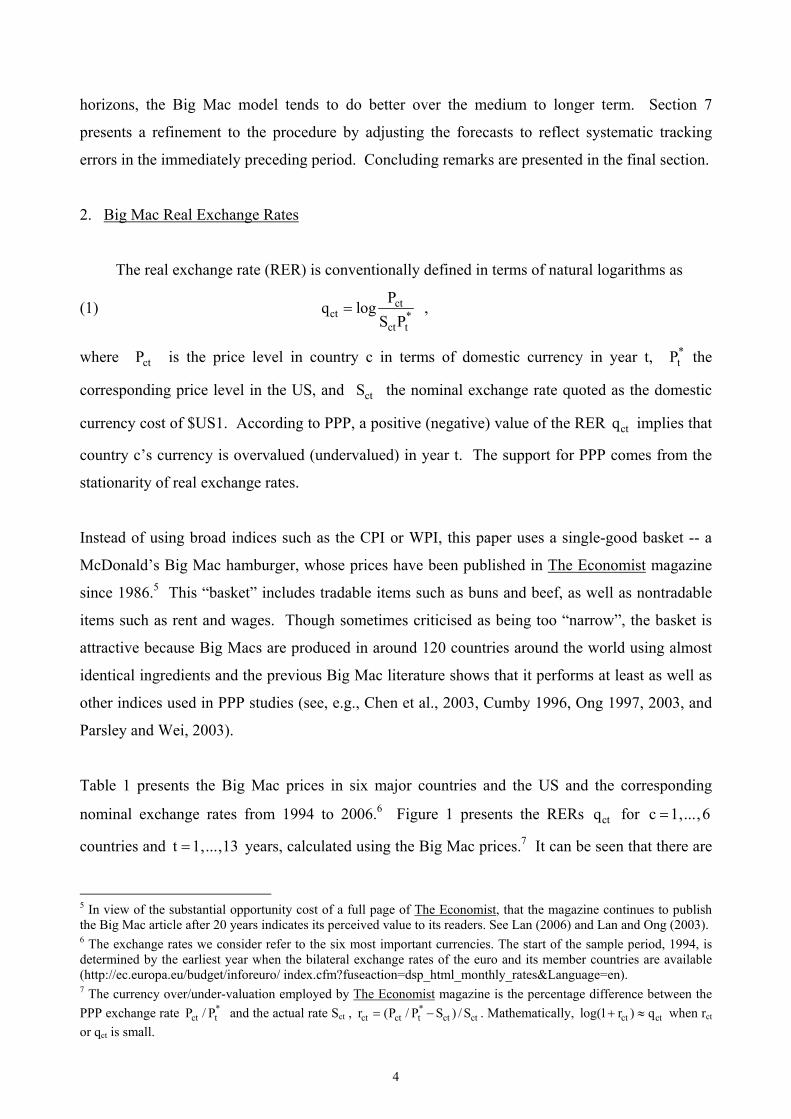
2. Big Mac Real Exchange Rates
The real exchange rate (RER) is conventionally defined in terms of natural logarithms as
(1) ctct *
ct t
Pq logS P
= ,
where ctP is the price level in country c in terms of domestic currency in year t, *tP the
corresponding price level in the US, and ctS the nominal exchange rate quoted as the domestic
currency cost of $US1. According to PPP, a positive (negative) value of the RER ctq implies that
country c’s currency is overvalued (undervalued) in year t. The support for PPP comes from the
stationarity of real exchange rates.
Instead of using broad indices such as the CPI or WPI, this paper uses a single-good basket -- a
McDonald’s Big Mac hamburger, whose prices have been published in The Economist magazine
since 1986.5 This “basket” includes tradable items such as buns and beef, as well as nontradable
items such as rent and wages. Though sometimes criticised as being too “narrow”, the basket is
attractive because Big Macs are produced in around 120 countries around the world using almost
identical ingredients and the previous Big Mac literature shows that it performs at least as well as
other indices used in PPP studies (see, e.g., Chen et al., 2003, Cumby 1996, Ong 1997, 2003, and
Parsley and Wei, 2003).
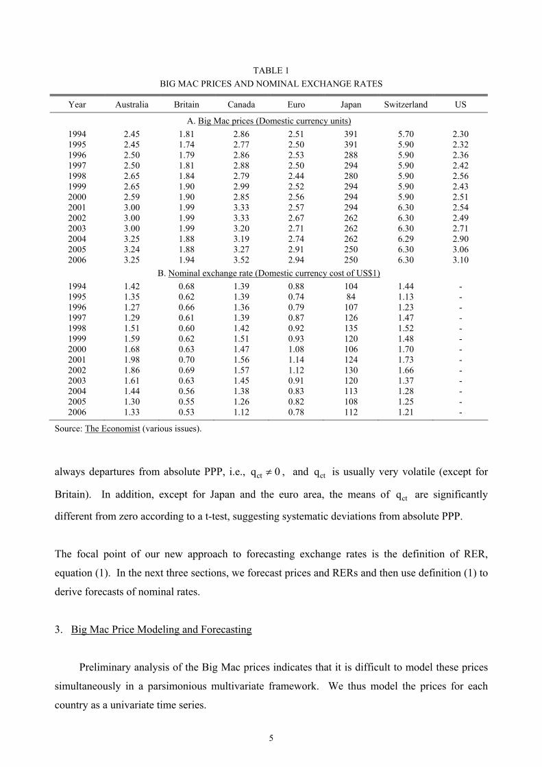
Table 1 presents the Big Mac prices in six major countries and the US and the corresponding
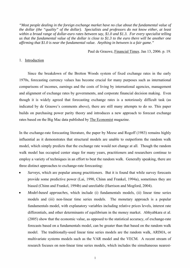
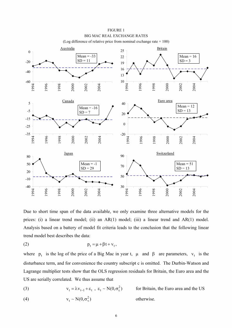
nominal exchange rates from 1994 to 2006.6 Figure 1 presents the RERs ctq for c 1,...,6=
countries and t 1,...,13= years, calculated using the Big Mac prices.7 It can be seen that there are
5 In view of the substantial opportunity cost of a full page of The Economist, that the magazine continues to publish the Big Mac article after 20 years indicates its perceived value to its readers. See Lan (2006) and Lan and Ong (2003). 6 The exchange rates we consider refer to the six most important currencies. The start of the sample period, 1994, is determined by the earliest year when the bilateral exchange rates of the euro and its member countries are available (http://ec.europa.eu/budget/inforeuro/ index.cfm?fuseaction=dsp_html_monthly_rates&Language=en). 7 The currency over/under-valuation employed by The Economist magazine is the percentage difference between the PPP exchange rate *
ct tP / P and the actual rate Sct , *ct ct t ct ctr (P / P S ) / S= − . Mathematically, ct ctlog(1 r ) q+ ≈ when rct
or qct is small.
5
TABLE 1 BIG MAC PRICES AND NOMINAL EXCHANGE RATES
Year Australia Britain Canada Euro Japan Switzerland US
A. Big Mac prices (Domestic currency units) 1994 2.45 1.81 2.86 2.51 391 5.70 2.30 1995 2.45 1.74 2.77 2.50 391 5.90 2.32 1996 2.50 1.79 2.86 2.53 288 5.90 2.36 1997 2.50 1.81 2.88 2.50 294 5.90 2.42 1998 2.65 1.84 2.79 2.44 280 5.90 2.56 1999 2.65 1.90 2.99 2.52 294 5.90 2.43 2000 2.59 1.90 2.85 2.56 294 5.90 2.51 2001 3.00 1.99 3.33 2.57 294 6.30 2.54 2002 3.00 1.99 3.33 2.67 262 6.30 2.49 2003 3.00 1.99 3.20 2.71 262 6.30 2.71 2004 3.25 1.88 3.19 2.74 262 6.29 2.90 2005 3.24 1.88 3.27 2.91 250 6.30 3.06 2006 3.25 1.94 3.52 2.94 250 6.30 3.10
B. Nominal exchange rate (Domestic currency cost of US$1) 1994 1.42 0.68 1.39 0.88 104 1.44 - 1995 1.35 0.62 1.39 0.74 84 1.13 - 1996 1.27 0.66 1.36 0.79 107 1.23 - 1997 1.29 0.61 1.39 0.87 126 1.47 - 1998 1.51 0.60 1.42 0.92 135 1.52 - 1999 1.59 0.62 1.51 0.93 120 1.48 - 2000 1.68 0.63 1.47 1.08 106 1.70 - 2001 1.98 0.70 1.56 1.14 124 1.73 - 2002 1.86 0.69 1.57 1.12 130 1.66 - 2003 1.61 0.63 1.45 0.91 120 1.37 - 2004 1.44 0.56 1.38 0.83 113 1.28 - 2005 1.30 0.55 1.26 0.82 108 1.25 - 2006 1.33 0.53 1.12 0.78 112 1.21 -
Source: The Economist (various issues). always departures from absolute PPP, i.e., ctq 0≠ , and ctq is usually very volatile (except for
Britain). In addition, except for Japan and the euro area, the means of ctq are significantly
different from zero according to a t-test, suggesting systematic deviations from absolute PPP.
The focal point of our new approach to forecasting exchange rates is the definition of RER,
equation (1). In the next three sections, we forecast prices and RERs and then use definition (1) to
derive forecasts of nominal rates.
3. Big Mac Price Modeling and Forecasting
Preliminary analysis of the Big Mac prices indicates that it is difficult to model these prices
simultaneously in a parsimonious multivariate framework. We thus model the prices for each
country as a univariate time series.
6
FIGURE 1 BIG MAC REAL EXCHANGE RATES
(Log difference of relative price from nominal exchange rate × 100)
Australia
-60
-40
-20
0
1994
1996
1998
2000
2002
2004
Britain
101316192225
1994
1996
1998
2000
2002
2004
Canada
-35
-25
-15
-5
5
1994
1996
1998
2000
2002
2004
Euro area
-20
0
20
40
1994
1996
1998
2000
2002
2004
Japan
-40
-10
20
50
80
1994
1996
1998
2000
2002
2004
Switzerland
30
50
70
90
1994
1996
1998
2000
2002
2004
Due to short time span of the data available, we only examine three alternative models for the
prices: (i) a linear trend model; (ii) an AR(1) model; (iii) a linear trend and AR(1) model.
Analysis based on a battery of model fit criteria leads to the conclusion that the following linear
trend model best describes the data:
(2) t tp t v= μ +β + ,
where tp is the log of the price of a Big Mac in year t, μ and β are parameters, tv is the
disturbance term, and for convenience the country subscript c is omitted. The Durbin-Watson and
Lagrange multiplier tests show that the OLS regression residuals for Britain, the Euro area and the
US are serially correlated. We thus assume that
(3) 2t t 1 t tv v , N(0, )− ε= λ + ε ε σ∼ for Britain, the Euro area and the US
(4) 2t vv N(0, )σ∼ otherwise.
Mean = -33 SD = 11
Mean = 16SD = 3
Mean = -16SD = 7
Mean = 12SD = 13
Mean = -1SD = 29
Mean = 51SD = 13
7
We then use the Cochrane-Orcutt method to estimate (2) and (3) for the Big Mac prices in the
above-mentioned three countries, and OLS to estimate (2) and (4) for those in the remaining four
countries.
Suppose that the forecast horizon is h years ahead of the last year of the sample period τ. One
attraction of using the linear trend model is that we can forecast the price at any forecast horizon h,
as the trend value h t= is not constrained to integer years, but can be a fraction of a year such as
one month, one week, one hour or even a few seconds. As discussed below, this has the
substantial advantage of allowing high-frequency forecasts that start with the most up-to-date
values of the actual exchange rate. To take forecast uncertainty into consideration, we use
Monte Carlo simulation techniques as follows. Let 2ˆ ˆˆ ˆ, , , εμ β λ σ and 2vσ̂ be the data-based
estimates of the corresponding parameters. In the jth trial ( j 1, ..., 10,000= replications),
according to (3) or (4) we generate an error term, denoted by ( j)hvτ+ , and then use equation (2) to
simulate 10,000 values of the price based on the estimates μ̂ and β̂ and the generated error
terms: ( j) ( j)h h
ˆˆp ( h) vτ+ τ+= μ +β τ + + , j 1, ..., 10,000= . The 10,000 forecasts of the price will be used
in Section 5 to obtain real-time forecasts of the nominal exchange rate of the country in question.
4. Real Exchange Rate Modeling and Forecasting
PPP theory implies that the RER has a constant mean and deviations from this constant are
temporary and dissipate over time. On the other hand, if PPP does not hold, the RER will have a
unit root, deviations from parity are cumulative and the RER does not have a well-defined centre
of gravity in the long run. Whether or not RERs are stationary has been a controversial issue in
the literature, but in the past decade there is mounting evidence that they are, so that PPP holds in
the long run. In this section, we first use the procedures introduced by Lan (2006) to model and
test the six Big Mac RERs in a seemingly-unrelated framework, and then extend the methodology
to accommodate non-integer forecast horizons.
We assume that the data-generating process for RERs is as follows:
(5) ct1t,ccct uqq +ρ+α=Δ − , c 1, ... ,6= , t 2, ... ,13= ,
where cα is the country-specific intercept, ρ is the common speed-of-adjustment parameter, and
ctu is a disturbance term with ctE(u ) 0= . As there are only 13 years of Big Mac data available,
8
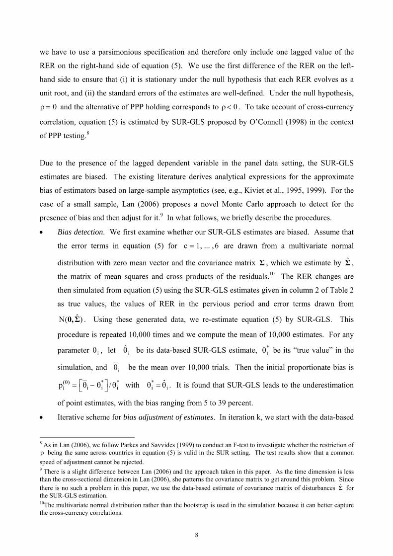
we have to use a parsimonious specification and therefore only include one lagged value of the
RER on the right-hand side of equation (5). We use the first difference of the RER on the left-
hand side to ensure that (i) it is stationary under the null hypothesis that each RER evolves as a
unit root, and (ii) the standard errors of the estimates are well-defined. Under the null hypothesis,
0=ρ and the alternative of PPP holding corresponds to 0<ρ . To take account of cross-currency
correlation, equation (5) is estimated by SUR-GLS proposed by O’Connell (1998) in the context
of PPP testing.8
Due to the presence of the lagged dependent variable in the panel data setting, the SUR-GLS
estimates are biased. The existing literature derives analytical expressions for the approximate
bias of estimators based on large-sample asymptotics (see, e.g., Kiviet et al., 1995, 1999). For the
case of a small sample, Lan (2006) proposes a novel Monte Carlo approach to detect for the
presence of bias and then adjust for it.9 In what follows, we briefly describe the procedures.
• Bias detection. We first examine whether our SUR-GLS estimates are biased. Assume that
the error terms in equation (5) for c 1, ... ,6= are drawn from a multivariate normal
distribution with zero mean vector and the covariance matrix Σ , which we estimate by Σ̂ ,
the matrix of mean squares and cross products of the residuals.10 The RER changes are
then simulated from equation (5) using the SUR-GLS estimates given in column 2 of Table 2
as true values, the values of RER in the pervious period and error terms drawn from
ˆN( )0,Σ . Using these generated data, we re-estimate equation (5) by SUR-GLS. This
procedure is repeated 10,000 times and we compute the mean of 10,000 estimates. For any
parameter iθ , let iθ̂ be its data-based SUR-GLS estimate, *iθ be its “true value” in the
simulation, and iθ be the mean over 10,000 trials. Then the initial proportionate bias is
(0) * *i i iip /⎡ ⎤= θ − θ θ⎣ ⎦ with *
i iˆθ = θ . It is found that SUR-GLS leads to the underestimation
of point estimates, with the bias ranging from 5 to 39 percent.
• Iterative scheme for bias adjustment of estimates. In iteration k, we start with the data-based
8 As in Lan (2006), we follow Parkes and Savvides (1999) to conduct an F-test to investigate whether the restriction of ρ being the same across countries in equation (5) is valid in the SUR setting. The test results show that a common speed of adjustment cannot be rejected. 9 There is a slight difference between Lan (2006) and the approach taken in this paper. As the time dimension is less than the cross-sectional dimension in Lan (2006), she patterns the covariance matrix to get around this problem. Since there is no such a problem in this paper, we use the data-based estimate of covariance matrix of disturbances Σ̂ for the SUR-GLS estimation. 10The multivariate normal distribution rather than the bootstrap is used in the simulation because it can better capture the cross-currency correlations.
9
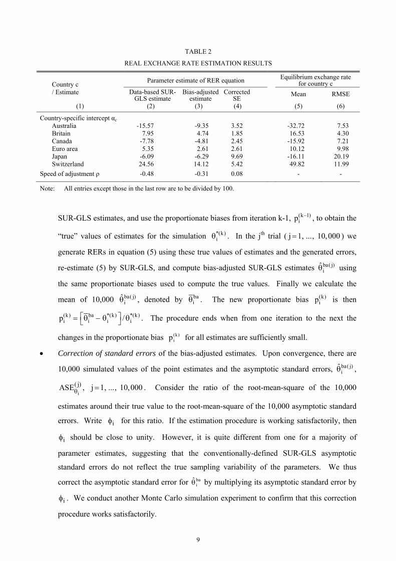
TABLE 2
REAL EXCHANGE RATE ESTIMATION RESULTS
Parameter estimate of RER equation Equilibrium exchange rate for country c Country c
/ Estimate Data-based SUR-GLS estimate
Bias-adjusted estimate
Corrected SE
Mean RMSE
(1) (2) (3) (4) (5) (6)
Country-specific intercept αc Australia -15.57 -9.35 3.52 -32.72 7.53 Britain 7.95 4.74 1.85 16.53 4.30 Canada -7.78 -4.81 2.45 -15.92 7.21 Euro area 5.35 2.61 2.61 10.12 9.98 Japan -6.09 -6.29 9.69 -16.11 20.19 Switzerland 24.56 14.12 5.42 49.82 11.99
Speed of adjustment ρ -0.48 -0.31 0.08 - -
Note: All entries except those in the last row are to be divided by 100.
SUR-GLS estimates, and use the proportionate biases from iteration k-1, (k 1)ip − , to obtain the
“true” values of estimates for the simulation *(k)iθ . In the jth trial ( j 1, ..., 10,000= ) we
generate RERs in equation (5) using these true values of estimates and the generated errors,
re-estimate (5) by SUR-GLS, and compute bias-adjusted SUR-GLS estimates ba( j)iθ̂ using
the same proportionate biases used to compute the true values. Finally we calculate the
mean of 10,000 ba( j)iθ̂ , denoted by ba
iθ . The new proportionate bias (k)ip is then
(k) ba *(k) *(k)ii i ip /⎡ ⎤= θ − θ θ⎣ ⎦ . The procedure ends when from one iteration to the next the
changes in the proportionate bias )k(ip for all estimates are sufficiently small.
• Correction of standard errors of the bias-adjusted estimates. Upon convergence, there are
10,000 simulated values of the point estimates and the asymptotic standard errors, ba( j)iθ̂ ,
i
( j)ASEθ , j 1, ..., 10,000= . Consider the ratio of the root-mean-square of the 10,000
estimates around their true value to the root-mean-square of the 10,000 asymptotic standard
errors. Write iφ for this ratio. If the estimation procedure is working satisfactorily, then
iφ should be close to unity. However, it is quite different from one for a majority of
parameter estimates, suggesting that the conventionally-defined SUR-GLS asymptotic
standard errors do not reflect the true sampling variability of the parameters. We thus
correct the asymptotic standard error for baiθ̂ by multiplying its asymptotic standard error by
iφ . We conduct another Monte Carlo simulation experiment to confirm that this correction
procedure works satisfactorily.
10
The bias-adjusted estimates and their corrected standard errors are presented in columns 3 and 4 of
Table 2. As can be seen, out of the seven estimates, only bacα̂ for c euro area= and Japan are not
significantly different from zero. To test whether the speed-of-adjustment parameter ρ is equal
to zero, we use the t statistic ba baˆ ˆ/ SE ( )τ = ρ ρ , which has a value of -3.98. As the iteration-
based estimate is used to calculate τ , the distribution of τ is non-standard under the null. We
thus derive its critical values by simulating 10,000 values of τ under the null; we then pick the
α-percentile of the 10,000 simulated values corresponding to the confidence interval (100 )−α
percent. The 1 percent, 5 percent and 10 percent critical values are –4.59, –3.68 and –3.09
respectively, suggesting that the unit root null is rejected at the 5 percent level.11
The conclusion of stationarity enables us to derive the long-run equilibrium value of the real
exchange rate for country c as Ec cq /= −α ρ , obtained by taking expectation of both sides of
equation (5). The estimated equilibrium exchange rate involves a ratio of estimated parameters,
but under normality such a ratio is typically not normally distributed and does not possess finite
moments.12 We thus employ a Monte Carlo simulation to measure the sampling variability of Ecq̂ ,
whose 10,000 estimated values follow directly from the bias-adjustment procedure described
above. The means and the root-mean-squared errors for the six equilibrium RERs are given in
columns 5 and 6 of Table 2. The ratio of the mean to the root-mean-squared error of Ecq̂ provides
a t-test on whether an equilibrium RER is significantly different from zero. These t-tests reveal
that in the long run, Australian and Canadian dollars are significantly undervalued, the British
pound and Swiss franc are overvalued, while the euro and Japanese yen are not significantly
different from parity. This result for the euro and yen agrees with Figure 1, where the means of
ctq for these two currencies tend not to be too far away from zero (and are not significantly
different therefrom).
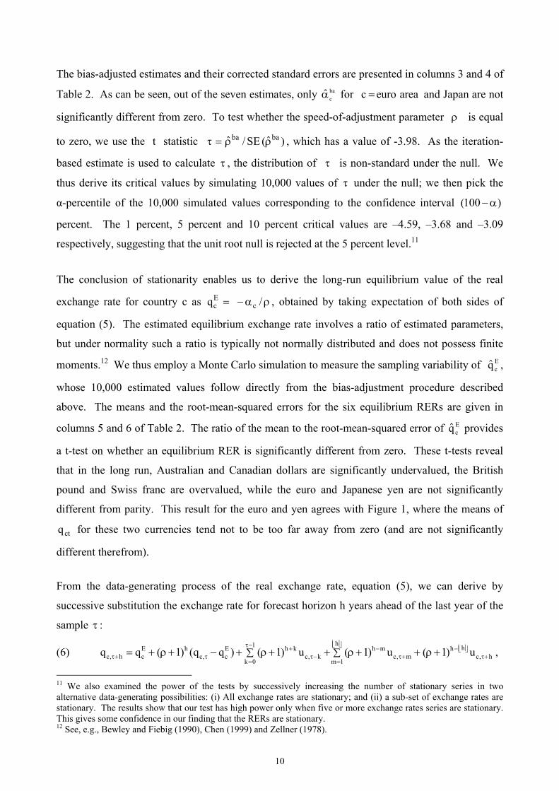
From the data-generating process of the real exchange rate, equation (5), we can derive by
successive substitution the exchange rate for forecast horizon h years ahead of the last year of the
sample τ :
(6) h1 hE h E h k h m h
c, h c c, c c, k c, m c, hk 0 m 1
q q ( 1) (q q ) ( 1) u ( 1) u ( 1) u⎢ ⎥τ− ⎣ ⎦ ⎢ ⎥+ − −⎣ ⎦
τ+ τ τ− τ+ τ+= =∑ ∑= + ρ+ − + ρ+ + ρ+ + ρ+ ,
11 We also examined the power of the tests by successively increasing the number of stationary series in two alternative data-generating possibilities: (i) All exchange rates are stationary; and (ii) a sub-set of exchange rates are stationary. The results show that our test has high power only when five or more exchange rates series are stationary. This gives some confidence in our finding that the RERs are stationary. 12 See, e.g., Bewley and Fiebig (1990), Chen (1999) and Zellner (1978).
11
where h can be non-integer and we use the floor function h ≡⎢ ⎥⎣ ⎦ greatest integer h≤ . The five
components on the right of equation (6) are as follows:
• The equilibrium exchange rate Ecq , to which the rate moves in the long run;
• The adjustment from the initial deviation ( Ec, cq qτ − ) with the adjustment speed ( 1ρ+ );
• A weighted sum of in-sample shocks, with the weight h k( 1) +ρ + being accorded to the shock
(h+k) years before the year ( hτ + );
• A weighted sum of out-of-sample shocks associated with forecast horizon integer years; and
• The final shock, the influence of which depends on the non-integer time interval, h h− ⎢ ⎥⎣ ⎦ .
To account for forecast uncertainty, we again use simulation techniques to forecast real exchange
rates based on equation (6). In each of 10,000 simulation experiments, we generate h⎢ ⎥⎣ ⎦ +1 error
terms for c 1, ... ,6= countries from a multivariate normal distribution with zero mean vector and
the data-based estimate of the covariance matrix Σ̂ . The 10,000 simulated values of the real
exchange rate for country c are obtained using equation (6) based on the biased-adjusted estimate
of ρ, the corresponding estimated Ecq and the generated shocks. In the next section, we merge
these RERs with the 10,000 forecast Big Mac prices to obtain real-time forecasts of the nominal
exchange rate.
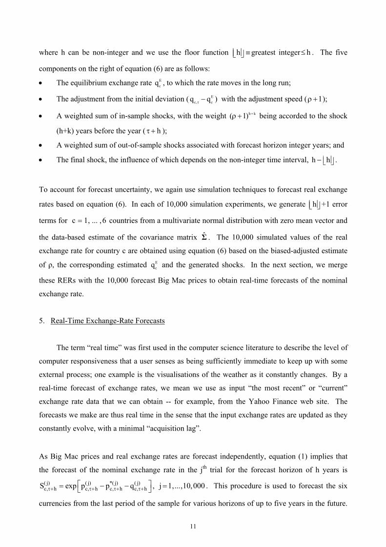
5. Real-Time Exchange-Rate Forecasts
The term “real time” was first used in the computer science literature to describe the level of
computer responsiveness that a user senses as being sufficiently immediate to keep up with some
external process; one example is the visualisations of the weather as it constantly changes. By a
real-time forecast of exchange rates, we mean we use as input “the most recent” or “current”
exchange rate data that we can obtain -- for example, from the Yahoo Finance web site. The
forecasts we make are thus real time in the sense that the input exchange rates are updated as they
constantly evolve, with a minimal “acquisition lag”.
As Big Mac prices and real exchange rates are forecast independently, equation (1) implies that
the forecast of the nominal exchange rate in the jth trial for the forecast horizon of h years is ( j) ( j) *( j) ( j)c, h c, h c, h c, hS exp p p qτ+ τ+ τ+ τ+⎡ ⎤= − −⎣ ⎦ , j 1,...,10,000= . This procedure is used to forecast the six
currencies from the last period of the sample for various horizons of up to five years in the future.
12
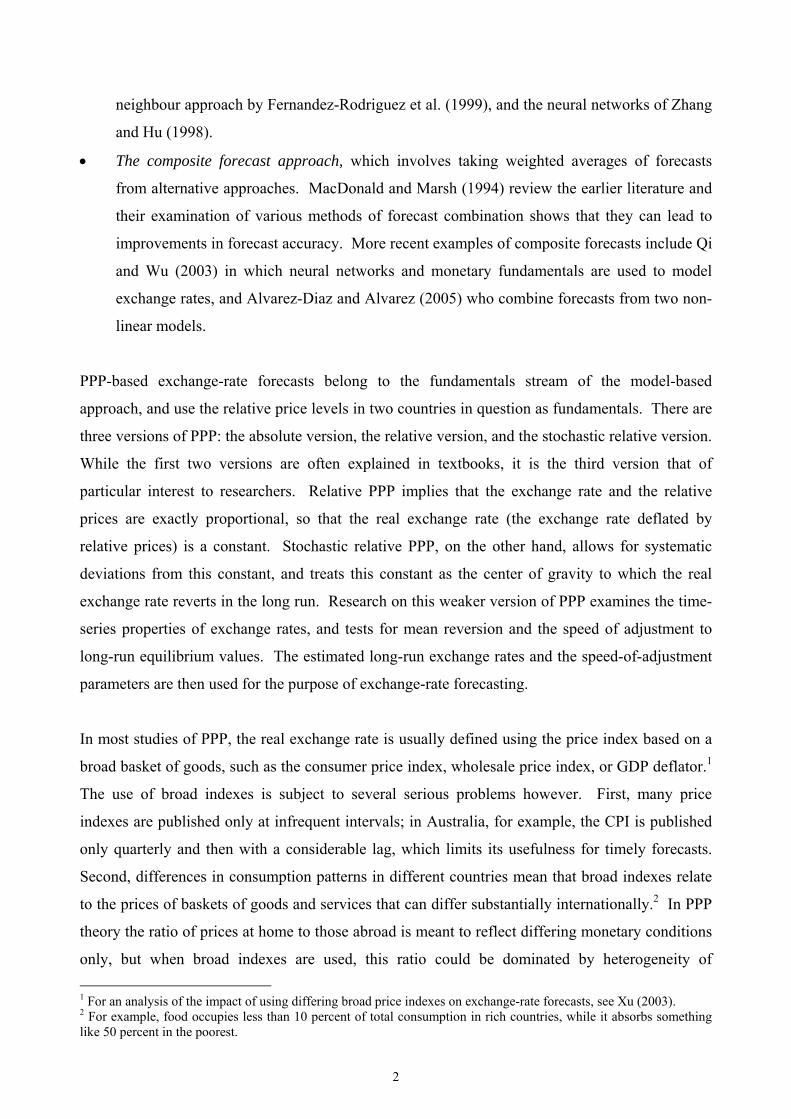
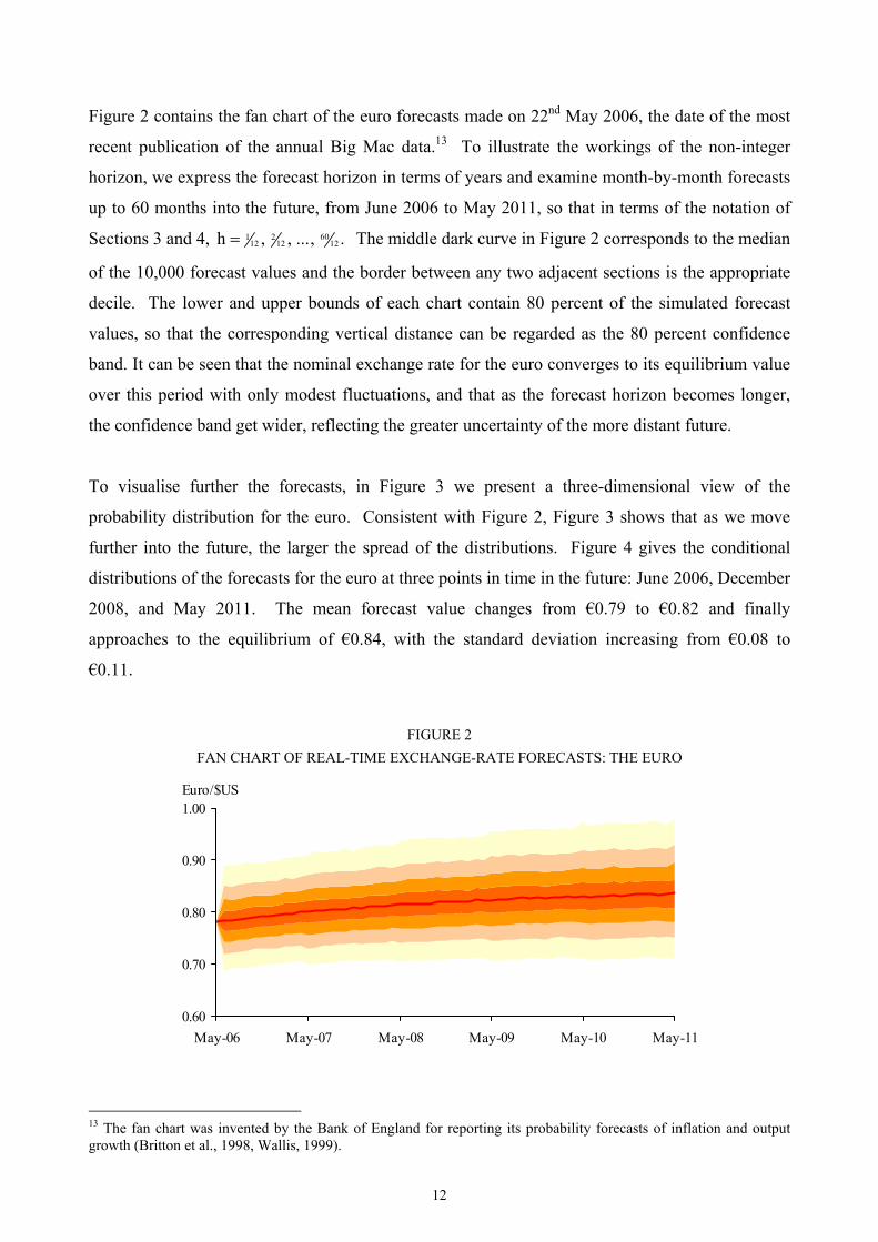
Figure 2 contains the fan chart of the euro forecasts made on 22nd May 2006, the date of the most
recent publication of the annual Big Mac data.13 To illustrate the workings of the non-integer
horizon, we express the forecast horizon in terms of years and examine month-by-month forecasts
up to 60 months into the future, from June 2006 to May 2011, so that in terms of the notation of
Sections 3 and 4, 601 212 12 12h , , ..., .= The middle dark curve in Figure 2 corresponds to the median
of the 10,000 forecast values and the border between any two adjacent sections is the appropriate
decile. The lower and upper bounds of each chart contain 80 percent of the simulated forecast
values, so that the corresponding vertical distance can be regarded as the 80 percent confidence
band. It can be seen that the nominal exchange rate for the euro converges to its equilibrium value
over this period with only modest fluctuations, and that as the forecast horizon becomes longer,
the confidence band get wider, reflecting the greater uncertainty of the more distant future.
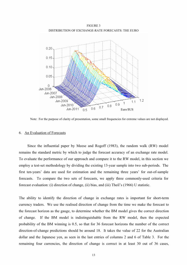
To visualise further the forecasts, in Figure 3 we present a three-dimensional view of the
probability distribution for the euro. Consistent with Figure 2, Figure 3 shows that as we move
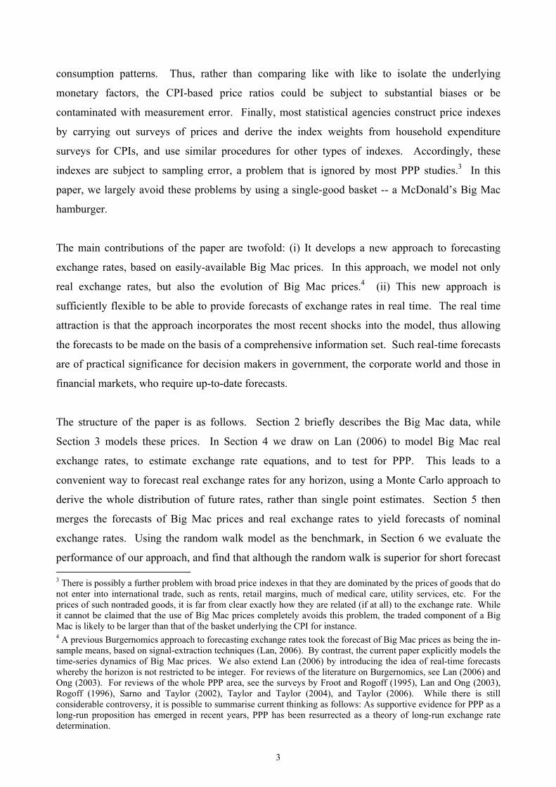
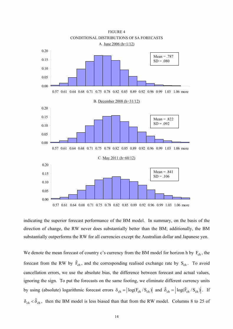
further into the future, the larger the spread of the distributions. Figure 4 gives the conditional
distributions of the forecasts for the euro at three points in time in the future: June 2006, December
2008, and May 2011. The mean forecast value changes from €0.79 to €0.82 and finally
approaches to the equilibrium of €0.84, with the standard deviation increasing from €0.08 to
€0.11.
FIGURE 2 FAN CHART OF REAL-TIME EXCHANGE-RATE FORECASTS: THE EURO
0.60
0.70
0.80
0.90
1.00
May-06 May-07 May-08 May-09 May-10 May-11
Euro/$US
13 The fan chart was invented by the Bank of England for reporting its probability forecasts of inflation and output growth (Britton et al., 1998, Wallis, 1999).
13
FIGURE 3 DISTRIBUTION OF EXCHANGE-RATE FORECASTS: THE EURO
Note: For the purpose of clarity of presentation, some small frequencies for extreme values are not displayed.
6. An Evaluation of Forecasts
Since the influential paper by Meese and Rogoff (1983), the random walk (RW) model
remains the standard metric by which to judge the forecast accuracy of an exchange rate model.
To evaluate the performance of our approach and compare it to the RW model, in this section we
employ a test-set methodology by dividing the existing 13-year sample into two sub-periods. The
first ten-years’ data are used for estimation and the remaining three years’ for out-of-sample
forecasts. To compare the two sets of forecasts, we apply three commonly-used criteria for
forecast evaluation: (i) direction of change, (ii) bias, and (iii) Theil’s (1966) U statistic.
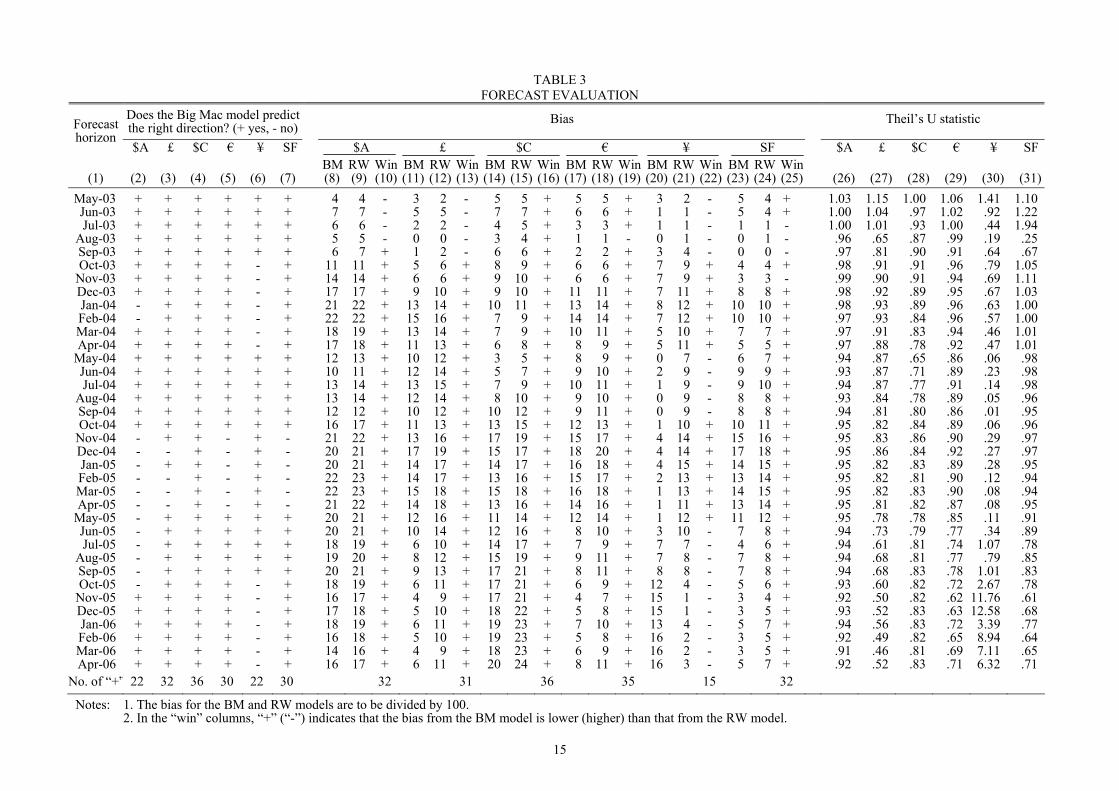
The ability to identify the direction of change in exchange rates is important for short-term
currency traders. We use the realised direction of change from the time we make the forecast to
the forecast horizon as the gauge, to determine whether the BM model gives the correct direction
of change. If the BM model is indistinguishable from the RW model, then the expected
probability of the BM winning is 0.5, so that for 36 forecast horizons the number of the correct
direction-of-change predictions should be around 18. It takes the value of 22 for the Australian
dollar and the Japanese yen, as seen in the last entries of columns 2 and 6 of Table 3. For the
remaining four currencies, the direction of change is correct in at least 30 out of 36 cases,
Euro/$US
14
FIGURE 4 CONDITIONAL DISTRIBUTIONS OF $A FORECASTS
A. June 2006 (h=1/12)
0.00
0.05
0.10
0.15
0.20
0.57 0.61 0.64 0.68 0.71 0.75 0.78 0.82 0.85 0.89 0.92 0.96 0.99 1.03 1.06 more
B. December 2008 (h=31/12)
0.00
0.05
0.10
0.15
0.20
0.57 0.61 0.64 0.68 0.71 0.75 0.78 0.82 0.85 0.89 0.92 0.96 0.99 1.03 1.06 more
C. May 2011 (h=60/12)
0.00
0.05
0.10
0.15
0.20
0.57 0.61 0.64 0.68 0.71 0.75 0.78 0.82 0.85 0.89 0.92 0.96 0.99 1.03 1.06 more
indicating the superior forecast performance of the BM model. In summary, on the basis of the
direction of change, the RW never does substantially better than the BM; additionally, the BM
substantially outperforms the RW for all currencies except the Australian dollar and Japanese yen.
We denote the mean forecast of country c’s currency from the BM model for horizon h by chF , the
forecast from the RW by chF , and the corresponding realised exchange rate by chS . To avoid
cancellation errors, we use the absolute bias, the difference between forecast and actual values,
ignoring the sign. To put the forecasts on the same footing, we eliminate different currency units
by using (absolute) logarithmic forecast errors ch ch chlog(F / S )δ = and ch ch chlog(F / S )δ = . If
ch chδ < δ , then the BM model is less biased than that from the RW model. Columns 8 to 25 of
Mean = .787 SD = .080
Mean = .841 SD = .106
Mean = .822 SD = .092
15
TABLE 3 FORECAST EVALUATION
Does the Big Mac model predict the right direction? (+ yes, - no)
Bias Theil’s U statistic Forecast horizon
$A £ $C € ¥ SF $A £ $C € ¥ SF $A £ $C € ¥ SF BM RW Win BM RW Win BM RW Win BM RW Win BM RW Win BM RW Win
(1) (2) (3) (4) (5) (6) (7) (8) (9) (10) (11) (12) (13) (14) (15) (16) (17) (18) (19) (20) (21) (22) (23) (24) (25) (26) (27) (28) (29) (30) (31) May-03 + + + + + + 4 4 - 3 2 - 5 5 + 5 5 + 3 2 - 5 4 + 1.03 1.15 1.00 1.06 1.41 1.10 Jun-03 + + + + + + 7 7 - 5 5 - 7 7 + 6 6 + 1 1 - 5 4 + 1.00 1.04 .97 1.02 .92 1.22 Jul-03 + + + + + + 6 6 - 2 2 - 4 5 + 3 3 + 1 1 - 1 1 - 1.00 1.01 .93 1.00 .44 1.94
Aug-03 + + + + + + 5 5 - 0 0 - 3 4 + 1 1 - 0 1 - 0 1 - .96 .65 .87 .99 .19 .25 Sep-03 + + + + + + 6 7 + 1 2 - 6 6 + 2 2 + 3 4 - 0 0 - .97 .81 .90 .91 .64 .67 Oct-03 + + + + - + 11 11 + 5 6 + 8 9 + 6 6 + 7 9 + 4 4 + .98 .91 .91 .96 .79 1.05
Nov-03 + + + + - + 14 14 + 6 6 + 9 10 + 6 6 + 7 9 + 3 3 - .99 .90 .91 .94 .69 1.11 Dec-03 + + + + - + 17 17 + 9 10 + 9 10 + 11 11 + 7 11 + 8 8 + .98 .92 .89 .95 .67 1.03 Jan-04 - + + + - + 21 22 + 13 14 + 10 11 + 13 14 + 8 12 + 10 10 + .98 .93 .89 .96 .63 1.00 Feb-04 - + + + - + 22 22 + 15 16 + 7 9 + 14 14 + 7 12 + 10 10 + .97 .93 .84 .96 .57 1.00 Mar-04 + + + + - + 18 19 + 13 14 + 7 9 + 10 11 + 5 10 + 7 7 + .97 .91 .83 .94 .46 1.01 Apr-04 + + + + - + 17 18 + 11 13 + 6 8 + 8 9 + 5 11 + 5 5 + .97 .88 .78 .92 .47 1.01
May-04 + + + + + + 12 13 + 10 12 + 3 5 + 8 9 + 0 7 - 6 7 + .94 .87 .65 .86 .06 .98 Jun-04 + + + + + + 10 11 + 12 14 + 5 7 + 9 10 + 2 9 - 9 9 + .93 .87 .71 .89 .23 .98 Jul-04 + + + + + + 13 14 + 13 15 + 7 9 + 10 11 + 1 9 - 9 10 + .94 .87 .77 .91 .14 .98
Aug-04 + + + + + + 13 14 + 12 14 + 8 10 + 9 10 + 0 9 - 8 8 + .93 .84 .78 .89 .05 .96 Sep-04 + + + + + + 12 12 + 10 12 + 10 12 + 9 11 + 0 9 - 8 8 + .94 .81 .80 .86 .01 .95 Oct-04 + + + + + + 16 17 + 11 13 + 13 15 + 12 13 + 1 10 + 10 11 + .95 .82 .84 .89 .06 .96
Nov-04 - + + - + - 21 22 + 13 16 + 17 19 + 15 17 + 4 14 + 15 16 + .95 .83 .86 .90 .29 .97 Dec-04 - - + - + - 20 21 + 17 19 + 15 17 + 18 20 + 4 14 + 17 18 + .95 .86 .84 .92 .27 .97 Jan-05 - + + - + - 20 21 + 14 17 + 14 17 + 16 18 + 4 15 + 14 15 + .95 .82 .83 .89 .28 .95 Feb-05 - - + - + - 22 23 + 14 17 + 13 16 + 15 17 + 2 13 + 13 14 + .95 .82 .81 .90 .12 .94 Mar-05 - - + - + - 22 23 + 15 18 + 15 18 + 16 18 + 1 13 + 14 15 + .95 .82 .83 .90 .08 .94 Apr-05 - - + - + - 21 22 + 14 18 + 13 16 + 14 16 + 1 11 + 13 14 + .95 .81 .82 .87 .08 .95
May-05 - + + + + + 20 21 + 12 16 + 11 14 + 12 14 + 1 12 + 11 12 + .95 .78 .78 .85 .11 .91 Jun-05 - + + + + + 20 21 + 10 14 + 12 16 + 8 10 + 3 10 - 7 8 + .94 .73 .79 .77 .34 .89 Jul-05 - + + + + + 18 19 + 6 10 + 14 17 + 7 9 + 7 7 - 4 6 + .94 .61 .81 .74 1.07 .78
Aug-05 - + + + + + 19 20 + 8 12 + 15 19 + 9 11 + 7 8 - 7 8 + .94 .68 .81 .77 .79 .85 Sep-05 - + + + + + 20 21 + 9 13 + 17 21 + 8 11 + 8 8 - 7 8 + .94 .68 .83 .78 1.01 .83 Oct-05 - + + + - + 18 19 + 6 11 + 17 21 + 6 9 + 12 4 - 5 6 + .93 .60 .82 .72 2.67 .78
Nov-05 + + + + - + 16 17 + 4 9 + 17 21 + 4 7 + 15 1 - 3 4 + .92 .50 .82 .62 11.76 .61 Dec-05 + + + + - + 17 18 + 5 10 + 18 22 + 5 8 + 15 1 - 3 5 + .93 .52 .83 .63 12.58 .68 Jan-06 + + + + - + 18 19 + 6 11 + 19 23 + 7 10 + 13 4 - 5 7 + .94 .56 .83 .72 3.39 .77 Feb-06 + + + + - + 16 18 + 5 10 + 19 23 + 5 8 + 16 2 - 3 5 + .92 .49 .82 .65 8.94 .64 Mar-06 + + + + - + 14 16 + 4 9 + 18 23 + 6 9 + 16 2 - 3 5 + .91 .46 .81 .69 7.11 .65 Apr-06 + + + + - + 16 17 + 6 11 + 20 24 + 8 11 + 16 3 - 5 7 + .92 .52 .83 .71 6.32 .71
No. of “+” 22 32 36 30 22 30 32 31 36 35 15 32
Notes: 1. The bias for the BM and RW models are to be divided by 100. 2. In the “win” columns, “+” (“-”) indicates that the bias from the BM model is lower (higher) than that from the RW model.
16
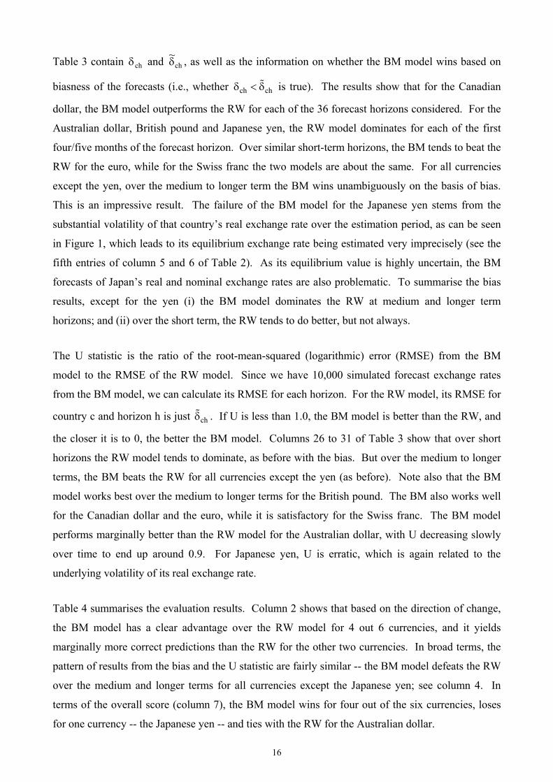
Table 3 contain chδ and ch~δ , as well as the information on whether the BM model wins based on
biasness of the forecasts (i.e., whether ch chδ < δ is true). The results show that for the Canadian
dollar, the BM model outperforms the RW for each of the 36 forecast horizons considered. For the
Australian dollar, British pound and Japanese yen, the RW model dominates for each of the first
four/five months of the forecast horizon. Over similar short-term horizons, the BM tends to beat the
RW for the euro, while for the Swiss franc the two models are about the same. For all currencies
except the yen, over the medium to longer term the BM wins unambiguously on the basis of bias.
This is an impressive result. The failure of the BM model for the Japanese yen stems from the
substantial volatility of that country’s real exchange rate over the estimation period, as can be seen
in Figure 1, which leads to its equilibrium exchange rate being estimated very imprecisely (see the
fifth entries of column 5 and 6 of Table 2). As its equilibrium value is highly uncertain, the BM
forecasts of Japan’s real and nominal exchange rates are also problematic. To summarise the bias
results, except for the yen (i) the BM model dominates the RW at medium and longer term
horizons; and (ii) over the short term, the RW tends to do better, but not always.
The U statistic is the ratio of the root-mean-squared (logarithmic) error (RMSE) from the BM
model to the RMSE of the RW model. Since we have 10,000 simulated forecast exchange rates
from the BM model, we can calculate its RMSE for each horizon. For the RW model, its RMSE for
country c and horizon h is just chδ . If U is less than 1.0, the BM model is better than the RW, and
the closer it is to 0, the better the BM model. Columns 26 to 31 of Table 3 show that over short
horizons the RW model tends to dominate, as before with the bias. But over the medium to longer
terms, the BM beats the RW for all currencies except the yen (as before). Note also that the BM
model works best over the medium to longer terms for the British pound. The BM also works well
for the Canadian dollar and the euro, while it is satisfactory for the Swiss franc. The BM model
performs marginally better than the RW model for the Australian dollar, with U decreasing slowly
over time to end up around 0.9. For Japanese yen, U is erratic, which is again related to the
underlying volatility of its real exchange rate.
Table 4 summarises the evaluation results. Column 2 shows that based on the direction of change,
the BM model has a clear advantage over the RW model for 4 out 6 currencies, and it yields
marginally more correct predictions than the RW for the other two currencies. In broad terms, the
pattern of results from the bias and the U statistic are fairly similar -- the BM model defeats the RW
over the medium and longer terms for all currencies except the Japanese yen; see column 4. In
terms of the overall score (column 7), the BM model wins for four out of the six currencies, loses
for one currency -- the Japanese yen -- and ties with the RW for the Australian dollar.
17
TABLE 4 SUMMARY OF FORECAST EVALUATION
Bias and U statistic Score Country /area
Direction of change
Short
horizons Medium and
longer horizons RW BM BM-RW
(1) (2) (3) (4) (5) (6) (7)=(6)-(5)
Australia BM≈RW RW wins BM wins 121 1
21 0 Britain BM wins RW wins BM wins 1 2 1 Canada BM wins BM wins BM wins 0 3 3 Euro area BM wins BM wins BM wins 0 3 3 Japan BM≈RW RW wins RW wins 1
22 12 -2
Switzerland BM wins BM≈RW BM wins 12 1
22 2
Note: For columns 5-6, we employ the scoring convention for the evaluation criteria of columns 2-4. We award the score of 1
2 if the two models are approximately the same and 1 (0) if the model in question wins (looses).
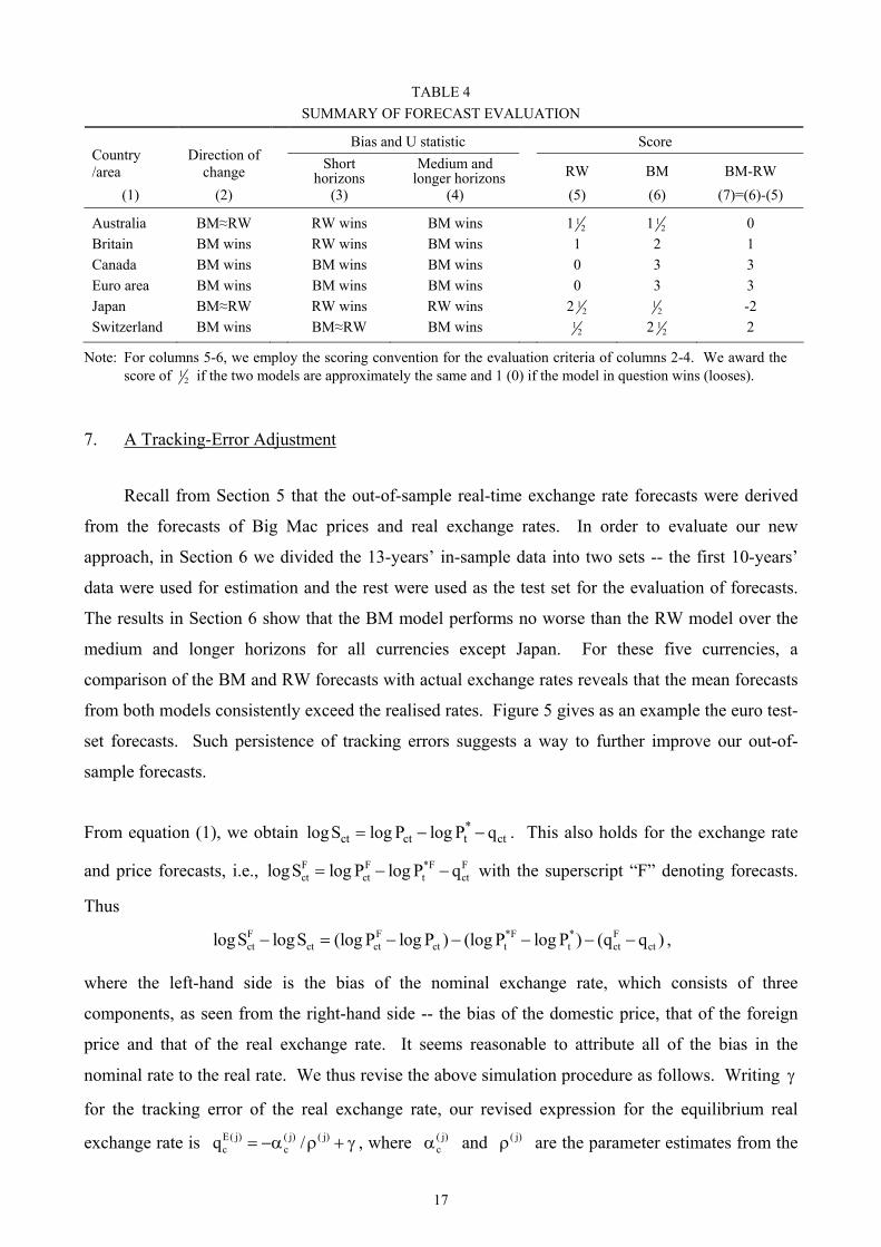
7. A Tracking-Error Adjustment
Recall from Section 5 that the out-of-sample real-time exchange rate forecasts were derived
from the forecasts of Big Mac prices and real exchange rates. In order to evaluate our new
approach, in Section 6 we divided the 13-years’ in-sample data into two sets -- the first 10-years’
data were used for estimation and the rest were used as the test set for the evaluation of forecasts.
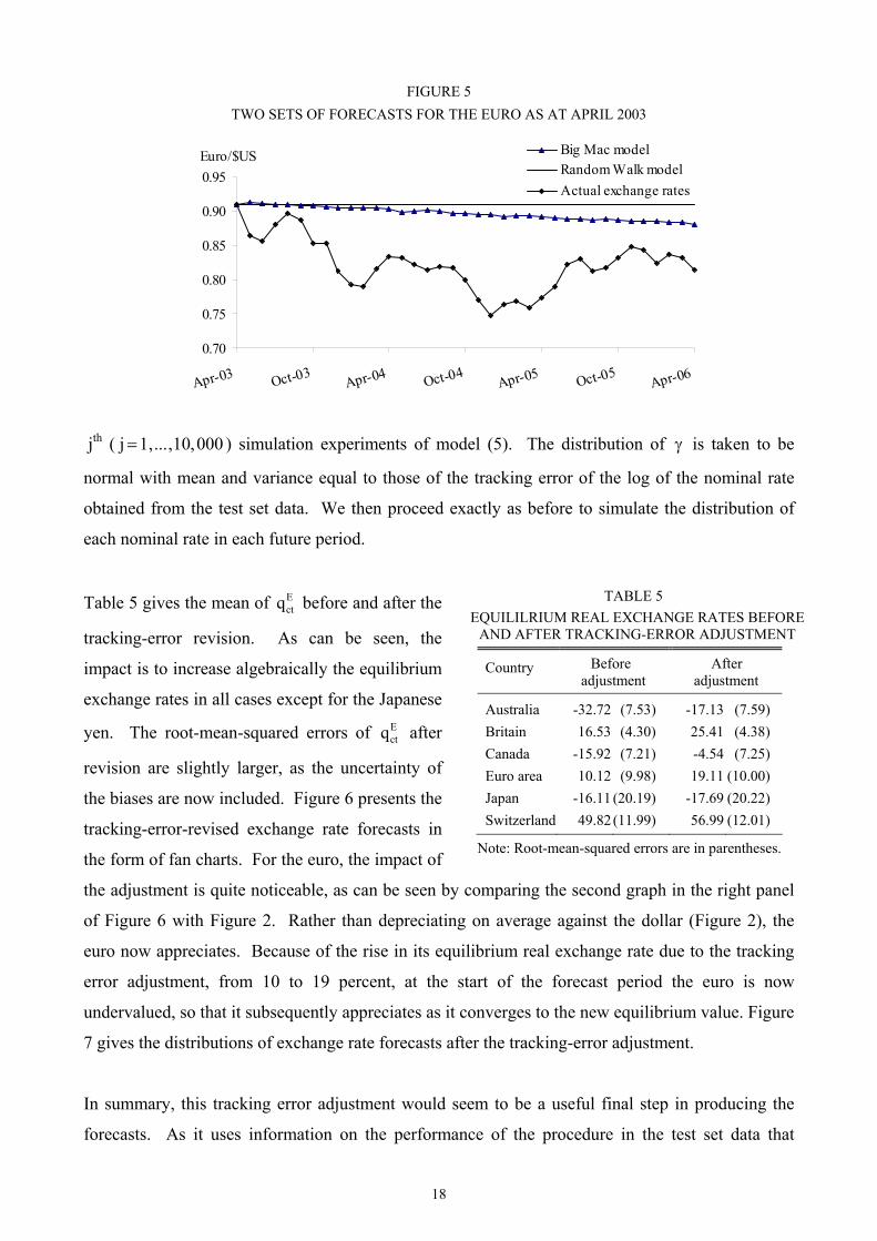
The results in Section 6 show that the BM model performs no worse than the RW model over the
medium and longer horizons for all currencies except Japan. For these five currencies, a
comparison of the BM and RW forecasts with actual exchange rates reveals that the mean forecasts
from both models consistently exceed the realised rates. Figure 5 gives as an example the euro test-
set forecasts. Such persistence of tracking errors suggests a way to further improve our out-of-
sample forecasts.
From equation (1), we obtain *ct ct t ctlogS log P log P q= − − . This also holds for the exchange rate
and price forecasts, i.e., F F *F Fct ct t ctlogS log P log P q= − − with the superscript “F” denoting forecasts.
Thus F F *F * Fct ct ct ct t t ct ctlogS logS (log P log P ) (log P log P ) (q q )− = − − − − − ,
where the left-hand side is the bias of the nominal exchange rate, which consists of three
components, as seen from the right-hand side -- the bias of the domestic price, that of the foreign
price and that of the real exchange rate. It seems reasonable to attribute all of the bias in the
nominal rate to the real rate. We thus revise the above simulation procedure as follows. Writing γ
for the tracking error of the real exchange rate, our revised expression for the equilibrium real
exchange rate is E( j) ( j) ( j)c cq /= −α ρ + γ , where ( j)
cα and ( j)ρ are the parameter estimates from the
18
FIGURE 5 TWO SETS OF FORECASTS FOR THE EURO AS AT APRIL 2003
0.70
0.75
0.80
0.85
0.90
0.95
Apr-03 Oct-03Apr-04 Oct-04
Apr-05 Oct-05Apr-06
Euro/$US Big Mac modelRandom Walk modelActual exchange rates
jth ( j 1,...,10,000= ) simulation experiments of model (5). The distribution of γ is taken to be
normal with mean and variance equal to those of the tracking error of the log of the nominal rate
obtained from the test set data. We then proceed exactly as before to simulate the distribution of
each nominal rate in each future period.
Table 5 gives the mean of Ectq before and after the
tracking-error revision. As can be seen, the
impact is to increase algebraically the equilibrium
exchange rates in all cases except for the Japanese
yen. The root-mean-squared errors of Ectq after
revision are slightly larger, as the uncertainty of
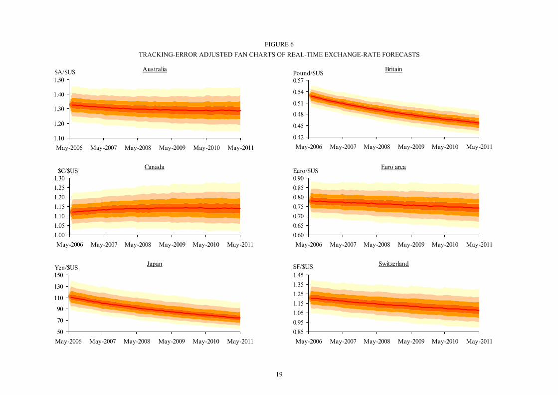
the biases are now included. Figure 6 presents the
tracking-error-revised exchange rate forecasts in
the form of fan charts. For the euro, the impact of
the adjustment is quite noticeable, as can be seen by comparing the second graph in the right panel
of Figure 6 with Figure 2. Rather than depreciating on average against the dollar (Figure 2), the
euro now appreciates. Because of the rise in its equilibrium real exchange rate due to the tracking
error adjustment, from 10 to 19 percent, at the start of the forecast period the euro is now
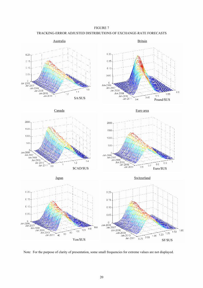
undervalued, so that it subsequently appreciates as it converges to the new equilibrium value. Figure
7 gives the distributions of exchange rate forecasts after the tracking-error adjustment.
In summary, this tracking error adjustment would seem to be a useful final step in producing the
forecasts. As it uses information on the performance of the procedure in the test set data that
TABLE 5 EQUILILRIUM REAL EXCHANGE RATES BEFORE
AND AFTER TRACKING-ERROR ADJUSTMENT
Country Before adjustment
After adjustment
Australia -32.72 (7.53) -17.13 (7.59) Britain 16.53 (4.30) 25.41 (4.38) Canada -15.92 (7.21) -4.54 (7.25) Euro area 10.12 (9.98) 19.11 (10.00) Japan -16.11 (20.19) -17.69 (20.22) Switzerland 49.82 (11.99) 56.99 (12.01)
Note: Root-mean-squared errors are in parentheses.
19
FIGURE 6 TRACKING-ERROR ADJUSTED FAN CHARTS OF REAL-TIME EXCHANGE-RATE FORECASTS
Australia
1.10
1.20
1.30
1.40
1.50
May-2006 May-2007 May-2008 May-2009 May-2010 May-2011
$A/$US
Britain
0.42
0.45
0.48
0.51
0.54
0.57
May-2006 May-2007 May-2008 May-2009 May-2010 May-2011
Pound/$US
Canada
1.001.051.101.151.201.251.30
May-2006 May-2007 May-2008 May-2009 May-2010 May-2011
$C/$US
Euro area
0.600.650.700.750.800.850.90
May-2006 May-2007 May-2008 May-2009 May-2010 May-2011
Euro/$US
Japan
50
70
90
110
130
150
May-2006 May-2007 May-2008 May-2009 May-2010 May-2011
Yen/$US
Switzerland
0.850.951.051.151.251.351.45
May-2006 May-2007 May-2008 May-2009 May-2010 May-2011
SF/$US
20
FIGURE 7 TRACKING-ERROR ADJUSTED DISTRIBUTIONS OF EXCHANGE-RATE FORECASTS
Australia
Britain
Canada
Euro area
Japan
Switzerland
Note: For the purpose of clarity of presentation, some small frequencies for extreme values are not displayed.
$A/$US Pound/$US
Euro/$US $CAD/$US
Yen/$US SF/$US
21
immediately proceeds the forecast period, this approach is consistent with the idea of
incorporating in the forecasts all of the most up-to-date information.
8. Concluding Comments
While forecasting exchange rates is a formidable task, the availability of Big Mac prices
provides a convenient way to make currency forecasts in real time. Rooted in purchasing power
parity theory, our Big Mac approach to forecasting exchange rates follows four steps:
(i) Time-series modelling of Big Mac prices to make price forecasts.
(ii) Testing for a unit root in real exchange rates in a seemingly-unrelated framework. Testing
and estimation are carried out in the context of bias-adjusted estimates and standard errors.
This model leads to estimates of equilibrium real exchange rates and forecasts of real
exchange rates.
(iii) Using a Monte Carlo simulation approach, the whole distribution of forecasts of nominal
exchange rates is then derived by merging the forecasts of the Big Mac prices and the real
exchange rates.
(iv) Based on the tracking errors of test-set forecasts, the out-of-sample forecasts are revised so
that they are unbiased.
The results shows that while the random walk model still dominates over the short forecast
horizons, i.e., within six months, the Big Mac model has a superior performance in forecasting
exchange rates over medium and long horizons.
Our approach to exchange-rate forecasting is attractive in three aspects. Firstly, it uses easily-
available Big Mac prices as input. These prices avoid several serious problems associated with
broad price indexes, such as the CPI, that are used in conventional PPP studies. Secondly, this
approach provides real-time exchange-rate forecasts at any forecast horizon. If required, such
real-time forecasts can be made on a day-to-day basis and adjust for recent tracking errors that
reflect swings in market sentiment. As these high-frequency forecasts are based on an up-to-date
and comprehensive information set, they could be particularly appealing to decision makers in
government, business and financial markets who want up-to-date forecasts of exchange rates.
Finally, as our forecasts are obtained through Monte Carlo simulation, estimation uncertainty is
made explicit in our framework which provides the entire distribution of future values of the
exchange rate, not just single point estimates. The dispersion of this distribution provides a
realistic measure of the riskiness of the forecasts.
22
References
Abhyankar, A., L. Sarno and G. Valente (2005). “Exchange Rates and Fundamentals: Evidence on the Economic Value of Predictability.” Journal of International Economics 66: 325-348.
Alvarez-Diaz, M. and A. Alvarez (2005). “Genetic Multi-model Composite Forecast for Non-linear Prediction of Exchange Rates.” Empirical Economics 30: 643-663.
Bewley, R. and D. G. Fiebig (1990). “Why are Long-Run Parameter Estimates So Disparate?” Review of Economics and Statistics 72: 345-349.
Britton, E., P. Fisher and J. Whitley (1998). “The Inflation Report Projections: Understanding the Fan Chart.” Bank of England Quarterly Bulletin 38: 30-37.
Chen, D.-L. (1999). World Consumption Economics. Singapore: World Scientific. Chen, C.-F., C.-H. Shen and C.-A. Wang (2003). “Big Mac PPP and Consumer Price PPP.”
Seminar Paper, National Taiwan University. Chinn, M. and J. Frankel (1994a). “More Survey Data on Exchange Rate Expectations: More
Currencies, More Horizons, More Tests.” Working Paper No. 312, Department of Economics, University of California, Santa Cruz.
Chinn, M. and J. Frankel (1994b). “Patterns in Exchange Rate Forecasts for Twenty-five Currencies.” Journal of Money, Credit, and Banking 26: 759-770.
Cumby, R. E. (1996). “Forecasting Exchange Rates and Relative Prices with the Hamburger Standard: Is What You Want What You Get with McParity?” NBER Research Paper 5675. National Bureau of Economic Research.
Fernandez-Rodriguez, F., S. Sosvilla-Rivero and J. Andrada-Felix (1999). “Exchange-Rate Forecasts with Simultaneous Nearest-Neighbour Methods: Evidence from the EMS.” International Journal of Forecasting 15: 383-392.
Froot, K. A. and K. Rogoff, (1995). “Perspectives on PPP and Long-Run Real Exchange Rates.” In G. M. Grossman and K. Rogoff (eds) Handbook of International Economics. Amsterdam: North-Holland Press. Pp. 1647-1688.
Harrison, S. and C. Mogford (2004). “Recent Developments in Surveys of Exchange Rate Forecasts.” Bank of England Quarterly Bulletin 44: 170-175.
Kiviet, J. F., G. D. A. Phillips and B. Schipp (1995). “The Bias of OLS, GLS, and ZEF Estimators in Dynamic Seemingly Unrelated Regression Models.” Journal of Econometrics 69: 241-266.
Kiviet, J. F., G. D. A. Phillips and B. Schipp (1999). “Alternative Bias Approximations in First-Order Dynamic Reduced Form Models.” Journal of Economic Dynamics and Control 23: 909-928.
Lai, K. S. (1990). “An Evaluation of Survey Exchange Rate Forecasts.” Economics Letters 32: 61-65.
Lan, Y. (2002). “The Explosion of Purchasing Power Parity.” In M. Manzur (ed) Exchange Rates, Interest Rates and Commodity Prices. Cheltenham, UK and Northampton, MA, USA: Edward Elgar Publishing. Pp. 9-39.
Lan, Y. (2006). “Equilibrium Exchange Rates and Currency Forecasts: A Big Mac Perspective.” International Economics and Finance Journal (forthcoming).
Lan, Y. and L. L. Ong (2003). “The Growing Evidence on Purchasing Power Parity.” In L. L. Ong The Big Mac Index: Applications of Purchasing Power Parity. UK: Palgrave MacMillan. Pp. 29-50.
23
MacDonald, R. and I. W. Marsh (1994). “Combining Exchange Rate forecasts: What is the Optimal Consensus Measure?” Journal of Forecasting 13: 313-332.
Meese, R. and K. Rogoff (1983). “Empirical Exchange Rate Models of the Seventies: Do They Fit Out of Sample?” Journal of International Economics 14: 3-24.
O’Connell, P. G. J. (1998). “The Overvaluation of Purchasing Power Parity.” Journal of International Economics 44: 1-19.
Ong, L. L. (1997). “Burgernomics: the Economics of the Big Mac Standard.” Journal of International Money and Finance 16: 865-878.
Ong, L. L. (2003). The Big Mac Index: Applications of Purchasing Power Parity. UK: Palgrave Macmillan.
Parkes, A. L. H. and A. Savvides (1999). “Purchasing Power Parity in the Long Run and Structural Breaks: Evidence from Real Sterling Exchange Rates.” Applied Financial Economics 9: 117-27.
Parsley, D. and S. Wei. (2003). “A Prism into the PPP Puzzle: The Micro-Foundations of Big Mac Real Exchange Rates.” NBER Working Paper 10074. National Bureau of Economic Research.
Qi, M. and Y. Wu (2003). “Nonlinear Prediction of Exchange Rates with Monetary Fundamentals.” Journal of Empirical Finance 10: 623-40.
Rogoff, K. (1996). “The Purchasing Power Parity Puzzle.” Journal of Economic Literature 34: 647-668.
Sarno, L. and M. Taylor (2002). “Purchasing Power Parity and the Real Exchange Rate.” IMF Staff Papers 49: 65-105.
Taylor, A. and M. P. Taylor (2004). “The Purchasing Power Parity Debate.” Journal of Economic Perspectives 18: 135-158.
Taylor, M. (2006). “Real Exchange Rates and Purchasing Power Parity: Mean Reversion in Economic Thought.” Applied Financial Economics 16: 1-17.
Theil, H. (1966). Applied Economic Forecasting. Amsterdam: North Holland. Wallis, K. F. (1999). “Asymmetric Density Forecasts of Inflation and the Bank of England’s Fan
Chart.” National Institute Economic Review 167: 106-12. Xu, Z. (2003). “Purchasing Power Parity, Price Indices, and Exchange Rate Forecasts.” Journal of
International Money and Finance 22: 105-130. Zellner, A. (1978). “Estimation of Functions of Population Means and Regression Coefficients
including Structural Coefficients: A Minimum Expected Loss (MELO) Approach.” Journal of Econometrics 8: 127-58.
Zhang, G. and M. Hu (1998). “Neural Network Forecasting of the British Pound/US dollar Exchange Rate.” International Journal of Management Science 26: 495-506.