A Mixed Observability Markov Decision Process Model forMusical Pitch

Pouyan Rafiei Fard rafieifard@ce.sharif.edu

Department of Computer Engineering, Sharif University of Technology, Tehran, IRAN

Keyvan Yahya kxy054@bham.ac.uk

School of Psychology, University of Birmingham, Birmingham, UK

Abstract

Partially observable Markov decision pro-cesses have been widely used to provide mod-els for real-world decision making problems.In this paper, we will provide a method inwhich a slightly different version of themcalled Mixed observability Markov decisionprocess, MOMDP, is going to join with ourproblem. Basically, we aim at offering a be-havioural model for interaction of intelligentagents with musical pitch environment andwe will show that how MOMDP can shedsome light on building up a decision makingmodel for musical pitch conveniently.

1. Introduction

Partially observable Markov decision processes(POMDPs) have been widely used to provide modelsfor real-world decision making problems. Theyprovide a mathematical framework to model the inter-action between the agent and its environment. One ofthe most notable characteristics of POMDPs is theirability to keep planning in dynamic environments andunder uncertainty (Ong et al., 2010). To our knowl-edge, only a few authors have previously mentionedMDPs and POMDPs in the field of computer music.Among them, we could mention (Martin et al. , 2010)who demonstrated the use of POMDPs to controlmusical behaviour in different conditions.

In this paper, we propose a novel model for inter-action of the agents with musical pitch environmentbased on a variant of POMDPs called mixed observ-ability Markov decision process (Ong et al., 2010).

In 5th International Workshop on Machine Learning andMusic, Edinburgh, Scotland, UK, 2012. Copyright 2012 bythe author(s)/owner(s).

First, we mention the theoretical background of ourwork. In section 3, we propose our model for musicalpitch based on MOMDPs. Section 4 addresses someimplementation issues and presents an experiment toevaluate our model. Finally, we make our concludingremarks and discuss about the prospective potentialdevelopments of this models and its applications.

2. The Basic Idea of MOMDP

Beside the standard models of POMDP, there is amodel called MOMDP that makes a slightly differentwith the former one. The latter is basically a factoredPOMDP which benefits from factorizing its states. Ina MOMDP model, a state s is factored into two dif-ferent variables x, y. So by writing s = (x, y) we meanthat s is consisted of two variables such that x standsfor fully observable state and y stands for partially ob-servable state. Thus having been factorized, we wouldhave a mixed system space S = X × Y where X is thestate of all values for x and either does Y for y.

st-1

ot-1

at-1

st

ot

yt-1

ot-1

at-1

yt

ot

xt-1 xt

st-1 st

Fig. 1. The standard POMDP model (left) and the MOMDP model (right).A MOMDP state s is factored into two variables: s = (x, y), where x isfully observable and y is partially observable.

model a MOMDP. In a MOMDP, the fully observable statecomponents are represented as a single state variable x,while the partially observable components are represented asanother state variable y. Thus (x, y) specifies the completesystem state, and the state space is factored as S = X × Y ,where X is the space of all possible values for x and Y isthe space of all possible values for y. In our AUV example,x represents the depth and the orientation (d, θ), and yrepresents the horizontal position p.Formally a MOMDP model is specified as a tuple

(X ,Y ,A,O, TX , TY , Z,R, γ). The conditional probabilityfunction TX (x, y, a, x

′) = p(x′|x, y, a) gives the probabilitythat the fully observable state variable has value x′ if therobot takes action a in state (x, y), and TY(x, y, a, x

′, y′) =p(y′|x, y, a, x′) gives the probability that the partially ob-servable state variable has value y′ if the robot takes actiona in state (x, y) and the fully observable state variable hasvalue x′. Compared with the standard POMDP model, theMOMDP model uses a factored state-space representationX × Y , with the corresponding probabilistic state-transitionfunctions TX and TY . All other aspects remain the same. SeeFig. 1 for a comparison.∗So far, the changes introduced by the MOMDP model

seem mostly notational. The computational advantages be-come apparent when we consider the belief space B. Sincethe state variable x is fully observable and known exactly, weonly need to maintain a belief bY , a probability distributionon the state variable y. Any belief b ∈ B on the completesystem state s = (x, y) is then represented as (x, bY). LetBY denote the space of all beliefs on y. We now associatewith each value x of the fully observable state variable abelief space for y: BY(x) = {(x, bY) | bY ∈ BY}. BY(x) isa subspace in B, and B is a union of these subspaces: B =⋃

x∈X BY(x). Observe that while B has |X ||Y| dimensions,where |X | and |Y| are the number of states in X andY , each BY(x) has only |Y| dimensions. Effectively werepresent the high-dimensional space B as a union of lower-dimensional subspaces. When the uncertainty in a system issmall, specifically, when |Y| is small, the MOMDP modelleads to dramatic improvement in computational efficiency,due to the reduced dimensionality of the space.Now consider how we would represent and execute a

∗A MOMDP can be regarded as an instance of dynamic Bayesiannetwork (DBN). Following the DBN methodology, we could factor x ory further, but this may lead to difficulty in value function representation.

MOMDP policy. As mentioned in Section II-A, a POMDPpolicy can be represented as a value function V (b) =maxα∈Γ(α · b), where Γ is a set of α-vectors. In a MOMDP,a belief is given by (x, bY), and the belief space B is unionof subspaces BY(x) for x ∈ X . Correspondingly, a MOMDPvalue function V (x, bY) is represented as a collection of α-vector sets: {ΓY(x) | x ∈ X}, where for each x, ΓY(x) is aset of α-vectors defined over BY(x). To evaluate V (x, bY),we first find the right α-vector set ΓY(x) using the x valueand then find the maximum α-vector from the set:

V (x, bY) = maxα∈ΓY(x)(α · bY). (3)

In general, any value function V (b) = maxα∈Γ(α · b) can berepresented in this new form, as stated in the theorem below.Theorem 1: Let B = ⋃

x∈X BY(x) be the belief space of aMOMDP with state space X×Y . If V (b) = maxα∈Γ(α·b) isany value function over B in the standard POMDP form, thenV (b) is equivalent to a MOMDP value function V ′(x, bY) =maxα∈ΓY (x)(α·bY) such that for any b = (x, bY) with b ∈ B,x ∈ X , and bY ∈ BY(x), V (b) = V ′(x, bY).†.Geometrically, each α-vector set ΓY(x) represents a re-

striction of the POMDP value function V (b) to the subspaceBY(x): Vx(bY) = maxα∈ΓY (x)(α · bY). In a MOMDP, wecompute only these lower-dimensional restrictions {Vx(bY) |x ∈ X}, because B is simply a union of subspaces BY(x)for x ∈ X .A comparison of (1) and (3) also indicates that (3) often

results in faster policy execution, because action selectioncan be performed more efficiently. First, each α-vector inΓY(x) has length |Y|, while each α-vector in Γ has length|X ||Y|. Furthermore, in a MOMDP value function, the α-vectors are partitioned into groups according to the valueof x. We only need to calculate the maximum over ΓY(x),which is potentially much smaller than Γ in size.In summary, by factoring out the fully and partially

observable state variables, a MOMDP model reveals theinternal structure of the belief space as a union of lower-dimensional subspaces. We want to exploit this structure andperform all operations on beliefs and value functions in theselower-dimensional subspaces rather than the original beliefspace. Before we describe the details of our algorithm, let usfirst look at how MOMDPs can be used to handle uncertaintycommonly encountered in robotic systems.

B. Modeling Robotic Tasks with MOMDPsSensor limitations are a major source of uncertainty in

robotic systems and are closely related to observability. If arobot’s state consists of several components, some are fullyobservable, possibly due to accurate sensing, but others arenot. This is a natural case for modeling with MOMDPs. Allfully observable components are grouped together and mod-eled by the variable x. The other components are modeledby the variable y.

†Due to space limitations, the proofs of all the theorems are providedin the full version of the paper, which will be available on-line at http://motion.comp.nus.edu.sg/papers/rss09.pdf

Figure 1. the Standard POMDP model (left) and theMOMDP model (right) in which a state is divided intoa fully-observable state x and a partially-observable statey (adapted from (Ong et al., 2010)).

arX

iv:1

206.

0855

v1 [

cs.A

I] 5

Jun

201

2

A Mixed Observability Markov Decision Process Model for Musical Pitch

3. The Proposed Model

From music theory, we know that any compound inter-val can be decomposed into some octaves and a simpleinterval which this idea can also be brought to anyother simple intervals. In our MOMDP-based model,the agent makes its decisions according to the statesthat it receives from the environment which is herethe musical pitch space. A MOMDP is denoted by thetuple (X,Y,A,O, Tx, Ty, Z,R, γ). The relationship be-tween these quantities and the musical concepts of ourmodel are given elaborately in the following.

At each time step the environment is in a state s ∈ Swhere s = (x, y) and x ∈ X is a fully observablestate whereas y ∈ Y is a partially observable one. Inour model, a fully observable state represents a musi-cal pitch in which the agent is having a precise esti-mate of its frequency at the time t plus the intervalthe agent is supposed to make. For the sake of sim-plicity, we only consider the natural musical pitchesand the main intervals not beyond the octave inter-val. So, we have S = {′C ′,′D′,′E′,′ F ′,′G′,′A′,′B′}×{′1st′,′ 2nd′,′ 3rd′, ..,′ 7th′}.A is the set of actions avail-able to the agent. Here an action a ∈ A stands for amaking a transition via a musical interval decompo-sition. In each state we define the possible actionswith a set of decompositions. Relatively, the environ-ment lies in partially observable states y ∈ Y as theintermediate state regarding which one of actions theagent makes. Technically, the space of partially ob-servable states is the same space for fully observablestates. The parameter O is a set of observations thatthe agent makes which is the possible values of this pa-rameter is the same as values from X and Y . Finally,The R parameter is R1γ+R2, where γ is the discountfactor while R1 is the reward for this first interval de-composition and R2 is the reward given to the secondone.

4. Experiment: Reinforcing patterns

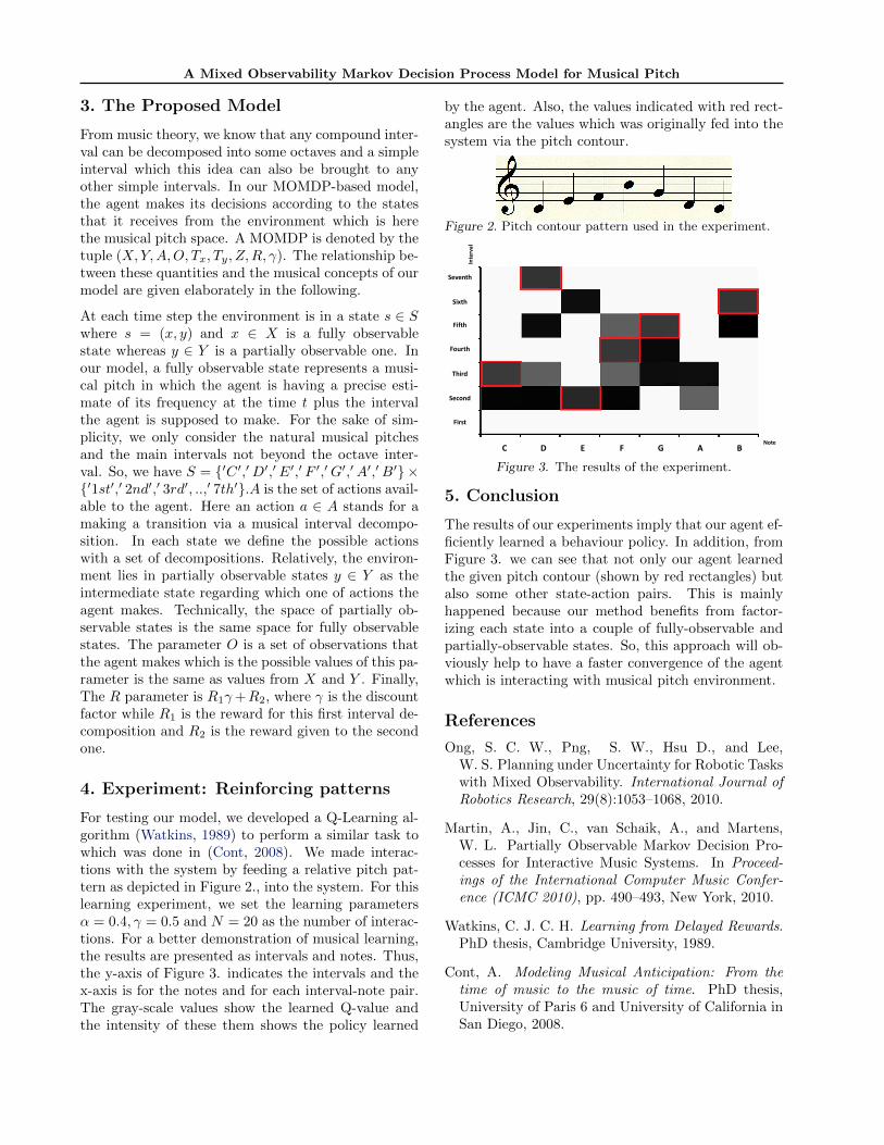
For testing our model, we developed a Q-Learning al-gorithm (Watkins, 1989) to perform a similar task towhich was done in (Cont, 2008). We made interac-tions with the system by feeding a relative pitch pat-tern as depicted in Figure 2., into the system. For thislearning experiment, we set the learning parametersα = 0.4, γ = 0.5 and N = 20 as the number of interac-tions. For a better demonstration of musical learning,the results are presented as intervals and notes. Thus,the y-axis of Figure 3. indicates the intervals and thex-axis is for the notes and for each interval-note pair.The gray-scale values show the learned Q-value andthe intensity of these them shows the policy learned

by the agent. Also, the values indicated with red rect-angles are the values which was originally fed into thesystem via the pitch contour.

Figure 2. Pitch contour pattern used in the experiment.

BAGFEDC

Seventh

Sixth

Fifth

Fourth

Third

Second

First

Note

Inte

rval

Figure 3. The results of the experiment.

5. Conclusion

The results of our experiments imply that our agent ef-ficiently learned a behaviour policy. In addition, fromFigure 3. we can see that not only our agent learnedthe given pitch contour (shown by red rectangles) butalso some other state-action pairs. This is mainlyhappened because our method benefits from factor-izing each state into a couple of fully-observable andpartially-observable states. So, this approach will ob-viously help to have a faster convergence of the agentwhich is interacting with musical pitch environment.

References

Ong, S. C. W., Png, S. W., Hsu D., and Lee,W. S. Planning under Uncertainty for Robotic Taskswith Mixed Observability. International Journal ofRobotics Research, 29(8):1053–1068, 2010.

Martin, A., Jin, C., van Schaik, A., and Martens,W. L. Partially Observable Markov Decision Pro-cesses for Interactive Music Systems. In Proceed-ings of the International Computer Music Confer-ence (ICMC 2010), pp. 490–493, New York, 2010.

Watkins, C. J. C. H. Learning from Delayed Rewards.PhD thesis, Cambridge University, 1989.

Cont, A. Modeling Musical Anticipation: From thetime of music to the music of time. PhD thesis,University of Paris 6 and University of California inSan Diego, 2008.