a mixed nite element formulation for incompressibility...
TRANSCRIPT
RUHR-UNIVERSITY BOCHUMFaculty for Civil Engineering
Institute for Structural Mechanics
Univ. Prof. Dr. techn. G. Meschke
Daniel Christ
A mixed finite element formulation forincompressibility using linear displacement
and pressure interpolations
Diploma Thesis – 5th of May 2003

Abstract
In this work shall be presented a stabilized finite element method to deal with incompress-ibility in solid mechanics. A mixed formulation involving pressure and displacement fieldsis used and a continuous linear interpolation is considered for both fields. To overcomethe Ladyzhenskaya-Babuska-Brezzi condition, a stabilization technique based on the or-thogonal sub-grid scale method is introduced. The main advantage of the method is thepossibility of using linear triangular finite elements, which are easy to generate for realindustrial applications. Results are compared with several improved formulations, as theenhanced assumed strain method (EAS) and the Q1P0-formulation, in nearly incompress-ible problems and in the context of linear elasticity and J2-plasticity.
Contents
1 Introduction 1
1.1 Motivation - locking of standard elements . . . . . . . . . . . . . . . . . . . 2
1.1.1 Locking in a bending dominated problem . . . . . . . . . . . . . . . 2
1.1.2 Locking in incompressibility . . . . . . . . . . . . . . . . . . . . . . 4
1.2 Object of the thesis . . . . . . . . . . . . . . . . . . . . . . . . . . . . . . . 5
1.3 Contents of the thesis . . . . . . . . . . . . . . . . . . . . . . . . . . . . . . 5
2 The Mixed Finite Element Formulation 7
2.1 Introduction . . . . . . . . . . . . . . . . . . . . . . . . . . . . . . . . . . . 7
2.2 The basic differential equations for mixed element formulations . . . . . . 8
2.3 The variational formulation for mixed finite elements . . . . . . . . . . . . 11
2.3.1 The weak form . . . . . . . . . . . . . . . . . . . . . . . . . . . . . 12
2.3.2 The matrix formulation . . . . . . . . . . . . . . . . . . . . . . . . 13
2.4 Illustration of a fundamental difficulty . . . . . . . . . . . . . . . . . . . . 15
2.5 The Mixed Patch Test . . . . . . . . . . . . . . . . . . . . . . . . . . . . . 16
2.5.1 Important properties of finite element solutions . . . . . . . . . . . 16
2.5.2 The basic requirements for mixed finite elements . . . . . . . . . . . 21
2.5.3 The derivation of the inf-sup-condition . . . . . . . . . . . . . . . . 22
2.5.4 Constraint counts . . . . . . . . . . . . . . . . . . . . . . . . . . . . 25
3 A Stabilized Mixed Element Formulation 29
3.1 Introduction . . . . . . . . . . . . . . . . . . . . . . . . . . . . . . . . . . . 29
3.2 The sub-grid-scale approach . . . . . . . . . . . . . . . . . . . . . . . . . . 29
3.2.1 The basic idea . . . . . . . . . . . . . . . . . . . . . . . . . . . . . 30
3.2.2 The orthogonal sub-scales . . . . . . . . . . . . . . . . . . . . . . . 33
3.2.3 Aspects to the stabilization of the mixed formulation in incom-pressibility . . . . . . . . . . . . . . . . . . . . . . . . . . . . . . . . 34
i
ii CONTENTS
3.3 Formulation in the elastic case . . . . . . . . . . . . . . . . . . . . . . . . 36
3.3.1 Constitutive model . . . . . . . . . . . . . . . . . . . . . . . . . . . 36
3.3.2 Formulation in the continuum . . . . . . . . . . . . . . . . . . . . . 37
3.3.3 Extension on multiscales . . . . . . . . . . . . . . . . . . . . . . . 40
3.3.4 Matrix formulation . . . . . . . . . . . . . . . . . . . . . . . . . . . 44
3.3.5 Implementation aspects . . . . . . . . . . . . . . . . . . . . . . . . 45
3.4 Formulation in the plastic case . . . . . . . . . . . . . . . . . . . . . . . . . 45
3.4.1 Constitutive model . . . . . . . . . . . . . . . . . . . . . . . . . . . 46
3.4.2 Formulation in the continuum . . . . . . . . . . . . . . . . . . . . . 47
3.4.3 Extension to multiscales . . . . . . . . . . . . . . . . . . . . . . . . 48
3.4.4 Implementation aspects . . . . . . . . . . . . . . . . . . . . . . . . 52
4 Numerical Results 55
4.1 Problems in case of elasticity . . . . . . . . . . . . . . . . . . . . . . . . . . 55
4.1.1 The patch test . . . . . . . . . . . . . . . . . . . . . . . . . . . . . 55
4.1.2 Forced cotter in plane strain . . . . . . . . . . . . . . . . . . . . . . 57
4.1.3 Driven cavity flow . . . . . . . . . . . . . . . . . . . . . . . . . . . . 59
4.2 Problems in case of plasticity . . . . . . . . . . . . . . . . . . . . . . . . . 62
4.2.1 Cook’s membrane . . . . . . . . . . . . . . . . . . . . . . . . . . . . 62
4.2.2 Compression of a 2D-block . . . . . . . . . . . . . . . . . . . . . . . 64
5 Conclusion 67
5.1 Summary . . . . . . . . . . . . . . . . . . . . . . . . . . . . . . . . . . . . 67
5.2 Statements . . . . . . . . . . . . . . . . . . . . . . . . . . . . . . . . . . . . 67
5.3 Aspects of future investigation . . . . . . . . . . . . . . . . . . . . . . . . . 68
Chapter 1
Introduction
The finite element method is a mathematic tool whose usage for the solving of variousproblems in physics or in engineering is getting more and more extended and important. Inengineering it will be actually integrated into the designing process of structures by usingseveral commercial programs. Simultaneously extended codes will be developed whichcan describe divers physical phenomena and its applications. Within the developmentof finite element methods the element formulation is an intensive investigation field ofits own, named element technology. The object of the element technology is to developrobust and efficient elements in view of the computational effort and the appliance togeneral problems. Series of desirable characteristics and requirements of finite elementscan be considered which should be fulfilled to reflect in an adequate way local problemsof solid mechanics:
• satisfying comportment in incompressible situations
• satisfying comportment in bending dominated problems
• little sensibility against distorted elements
• adequate precision in coarser meshes
• low computational cost
• applicable to triangular elements to simplify the mesh generation
• facility of the implementation of nonlinear constitutive models
Actually, in the practical applications it is tried to optimize low-order elements because oftheir simplicity, their efficiency and other advantageous aspects. The low-order elementsare less sensible against the distortion and as well produce a smaller bandwidth in theglobal matrix of the linear equation system which leads for example to a lower computa-tional cost and lesser need of memory.Nevertheless in the field of solid mechanics, elements of a low order like triangles or quadri-laterals with linear displacement interpolations turn out to present dissatisfied results as
1
2 CHAPTER 1: INTRODUCTION
a matter of extreme conditions such as in case of nearly incompressibility. In these casesthe numerical predictions that are obtained with these elements by using meshes whichare naturally adequate, differ significant of the physical response. Hence it is necessaryto know the causes which produce these insufficiencies and develop affording formulationsthat give an adequate result satisfying the physical response.
1.1 Motivation - locking of standard elements
The results that are obtained generally by using the standard displacement-based finiteelements are satisfactory for a great variety of problems. By formulating a continuumproblem via the finite element methods, a space of test functions is adopted. Essentially,what has to be done to find the solution of the given problem inside of the defined space isto introduce restrictions to the displacement solutions of the continuum problem wherebythe finite element method allows to find the best approximation in this space. Neverthe-less, in some situations exist proper restrictions of the medium which, established in thediscrete form, lead to an over restricted system. The space of the test functions emerges astoo poor for the problem and incapable to represent the deformations that have to occur.As a consequence the solution offered by this, in general under estimated function spacecould be nearly zero. This phenomenon is also known as locking. The locking of elementsare presented mostly in two different situations: on one hand in bending problems andon the other hand in case of incompressibility or nearly incompressibility, respectively.
1.1.1 Locking in a bending dominated problem
The standard linear elements are attractive because of their simplicity and the low com-putational cost by solving a problem. They offer the minimum number of nodes as wellas the minimum degrees of freedom. This restriction can effect an internal stiffness of theelement which is unknown to the physical conditions of the problem. Particularly in casesof bending dominated problems the linear elements offer unsatisfied results.In this type of problem the comparison between the theoretical displacement field andthe description by the linear element can show the difficulty of the problem. The purebending of an element as shown in Fig.1.1 leads to the following considerations.Let the displacement field in a bilinear element be described as
uj =
4∑
i=1
Ni(ξ, η) uij (1.1)
with the shape function
Ni(ξ, η) =1
4(1 + ξ ξi + η ηi + ξ ξi η ηi) (1.2)
1.1 Motivation - locking of standard elements 3
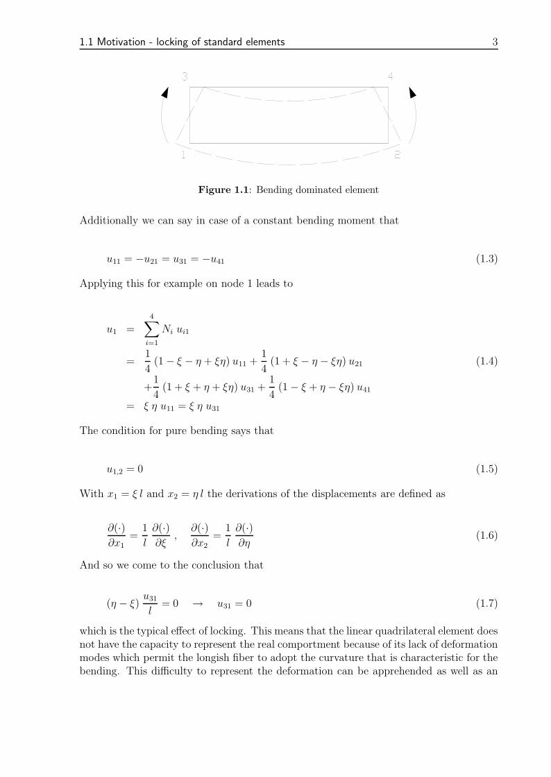
Figure 1.1: Bending dominated element
Additionally we can say in case of a constant bending moment that
u11 = −u21 = u31 = −u41 (1.3)
Applying this for example on node 1 leads to
u1 =4∑
i=1
Ni ui1
=1
4(1− ξ − η + ξη) u11 +
1
4(1 + ξ − η − ξη) u21 (1.4)
+1
4(1 + ξ + η + ξη) u31 +
1
4(1− ξ + η − ξη) u41
= ξ η u11 = ξ η u31
The condition for pure bending says that
u1,2 = 0 (1.5)
With x1 = ξ l and x2 = η l the derivations of the displacements are defined as
∂(·)
∂x1=
1
l
∂(·)
∂ξ,
∂(·)
∂x2=
1
l
∂(·)
∂η(1.6)
And so we come to the conclusion that
(η − ξ)u31
l= 0 → u31 = 0 (1.7)
which is the typical effect of locking. This means that the linear quadrilateral element doesnot have the capacity to represent the real comportment because of its lack of deformationmodes which permit the longish fiber to adopt the curvature that is characteristic for thebending. This difficulty to represent the deformation can be apprehended as well as an
4 CHAPTER 1: INTRODUCTION
extreme stiffness of the element.To delete or at least weaken the effect of locking, it could be refined the mesh size orimproved the elements quality to a higher order of interpolations for the displacementfield.
1.1.2 Locking in incompressibility
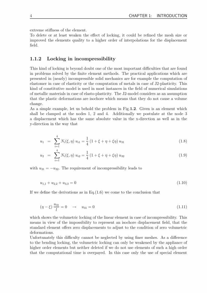
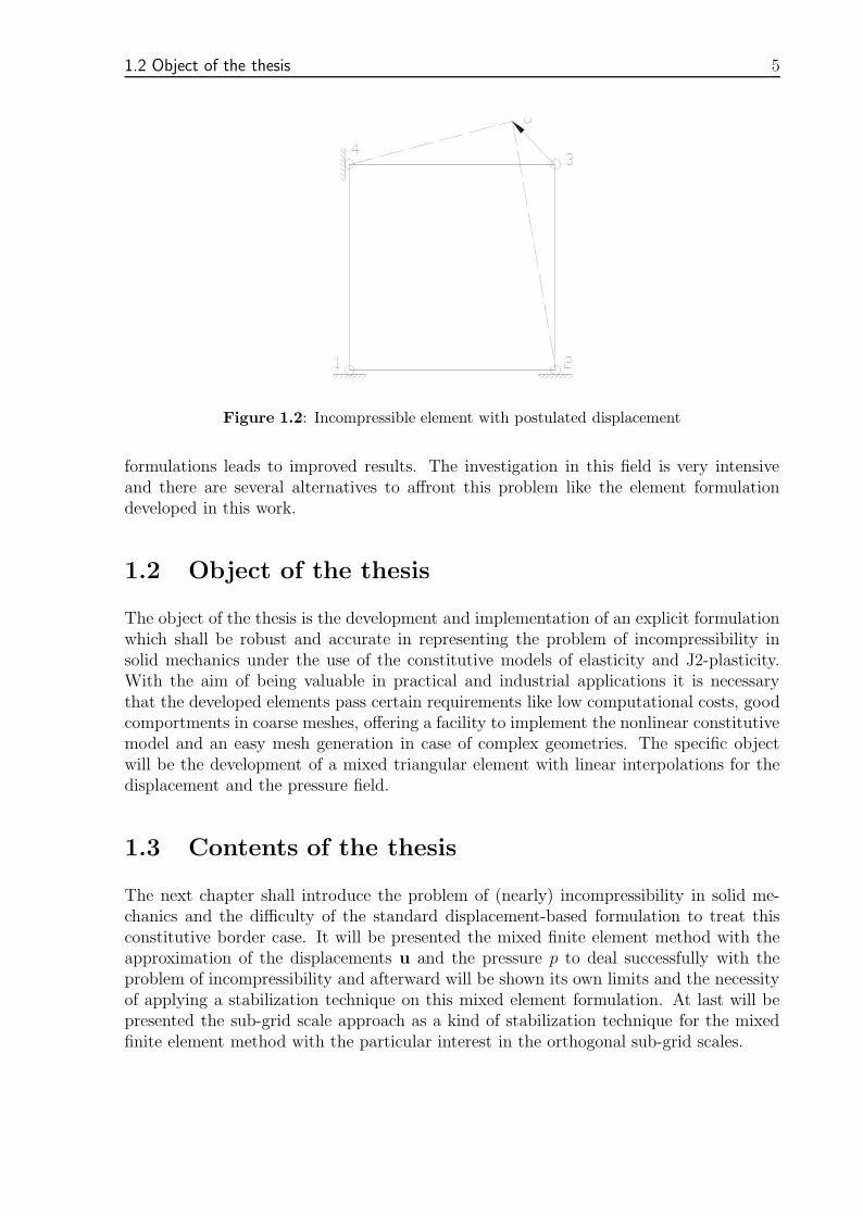
This kind of locking is beyond doubt one of the most important difficulties that are foundin problems solved by the finite element methods. The practical applications which arepresented in (nearly) incompressible solid mechanics are for example the computation ofelastomer in case of elasticity or the computation of metals in case of J2-plasticity. Thiskind of constitutive model is used in most instances in the field of numerical simulationsof metallic materials in case of elasto-plasticity. The J2-model considers as an assumptionthat the plastic deformations are isochore which means that they do not cause a volumechange.As a simple example, let us behold the problem in Fig.1.2. Given is an element whichshall be clamped at the nodes 1, 2 and 4. Additionally we postulate at the node 3a displacement which has the same absolute value in the x-direction as well as in they-direction in the way that
u1 =
4∑
i=1
Ni(ξ, η) ui1 =1
4(1 + ξ + η + ξη) u31 (1.8)
u2 =
4∑
i=1
Ni(ξ, η) ui2 =1
4(1 + ξ + η + ξη) u32 (1.9)
with u31 = −u32. The requirement of incompressibility leads to
u1,1 + u2,2 + u3,3 = 0 (1.10)
If we define the derivations as in Eq.(1.6) we come to the conclusion that
(η − ξ)u31
l= 0 → u31 = 0 (1.11)
which shows the volumetric locking of the linear element in case of incompressibility. Thismeans in view of the impossibility to represent an isochore displacement field, that thestandard element offers zero displacements to adjust to the condition of zero volumetricdeformations.Unfortunately this difficulty cannot be neglected by using finer meshes. As a differenceto the bending locking, the volumetric locking can only be weakened by the appliance ofhigher order elements but neither deleted if we do not use elements of such a high orderthat the computational time is overpayed. In this case only the use of special element
1.2 Object of the thesis 5
Figure 1.2: Incompressible element with postulated displacement
formulations leads to improved results. The investigation in this field is very intensiveand there are several alternatives to affront this problem like the element formulationdeveloped in this work.
1.2 Object of the thesis
The object of the thesis is the development and implementation of an explicit formulationwhich shall be robust and accurate in representing the problem of incompressibility insolid mechanics under the use of the constitutive models of elasticity and J2-plasticity.With the aim of being valuable in practical and industrial applications it is necessarythat the developed elements pass certain requirements like low computational costs, goodcomportments in coarse meshes, offering a facility to implement the nonlinear constitutivemodel and an easy mesh generation in case of complex geometries. The specific objectwill be the development of a mixed triangular element with linear interpolations for thedisplacement and the pressure field.
1.3 Contents of the thesis
The next chapter shall introduce the problem of (nearly) incompressibility in solid me-chanics and the difficulty of the standard displacement-based formulation to treat thisconstitutive border case. It will be presented the mixed finite element method with theapproximation of the displacements u and the pressure p to deal successfully with theproblem of incompressibility and afterward will be shown its own limits and the necessityof applying a stabilization technique on this mixed element formulation. At last will bepresented the sub-grid scale approach as a kind of stabilization technique for the mixedfinite element method with the particular interest in the orthogonal sub-grid scales.
6 CHAPTER 1: INTRODUCTION
In the third chapter will be developed a triangular mixed finite element formulation withlinear interpolations for the displacement and the pressure field stabilized by the previousspecified orthogonal sub-grid scale. It will be considered the case of elasticity as well asthe J2-plasticity.The fourth chapter treats of numerical results of this developed element in comparisonto other standard and enhanced finite element formulations like the standard quadrilat-eral and triangular elements, the EAS-element, the Q1P0-element and a triangular mixedelement without any stabilization. The comportment is shown by examples in cases ofelasticity and J2-plasticity.Finally conclusions of the thesis are drawn and possible future investigation aspects ofthis work will be emphasized.
Chapter 2
The Mixed Finite ElementFormulation
2.1 Introduction
Many problems of physical importance involve motions that essentially preserve volumeslocally. That means that after a deformation each small portion of the medium has thesame volume as before the deformation. Media that behave in this fashion are termedincompressible. In this case when the Poisson’s ratio ν becomes 0.5 the standard displace-ment formulation of elastic problems fails. Indeed, problems arise even when the materialis nearly incompressible with ν > 0.4 and the simple linear approximation with triangularelements gives highly oscillatory results in such cases.The application of a mixed formulation for such problems can avoid the difficulties andis of great practical interest as nearly incompressible behavior is encountered in a varietyof real engineering problems ranging from soil mechanics, as example the modeling ofclammy clay, to aerospace engineering where a usage of rubber like materials is funda-mental. Identical problems also arise when the flow of incompressible fluids is encounteredas in the case of Stoke’s flow.In this chapter the mixed approaches to incompressible problems shall be discussed, gen-erally using a two-field formulation where the displacements u and the pressure p are thefree variables. Such formulation allows the dealing with full incompressibility as well asnear incompressibility as it occurs. There are two ways to express this kind of two-fieldformulation with displacement and pressure variables which are very familiar. They differin the way of defining the pressure variable in the elements.
The u/p-formulation: In this formulation the pressure variable owns only to the justcontemplating element. These allows the static condensation of the pressure variable inevery element before they are assembled to the global structure which saves a lot of evalu-ation time. We will observe later on that this static condensation does not work for exactincompressibility (see section 2.3.2). The continuity of the pressure over the elements isnot forced but appears with the refining of the mesh.
7
8 CHAPTER 2: THE MIXED FINITE ELEMENT FORMULATION
The u/p-c formulation: This formulation assumes the continuity of the pressure overthe elements what means that the pressure is defined in the nodes of the elements whichare connected to neighboring elements. This excludes from the outset the static conden-sation of the pressure variables but leads to a continuous pressure field over the elementsindependent of the size of the mesh.
The question which element formulation is more efficient depends on the kind of problemthat has to be solved. Where the u/p-formulation is very fast in solving problems ofnearly incompressibility this property looses its function in exact incompressibility and ithas to be said that the results of the pressure can be very inaccurate if large meshes areused or extreme problems occur as it is demonstrated in chapter 4. The u/p-c formulationneeds particularly in case of nearly incompressibility more evaluation time but has theadvantage that the results of the pressure are very accurate. In the presented work shallbe developed a mixed finite element formulation based on a continuous u/p-formulationalso with the aim to circumvent the inaccuracy of the pressure distributions.
2.2 The basic differential equations for mixed ele-
ment formulations
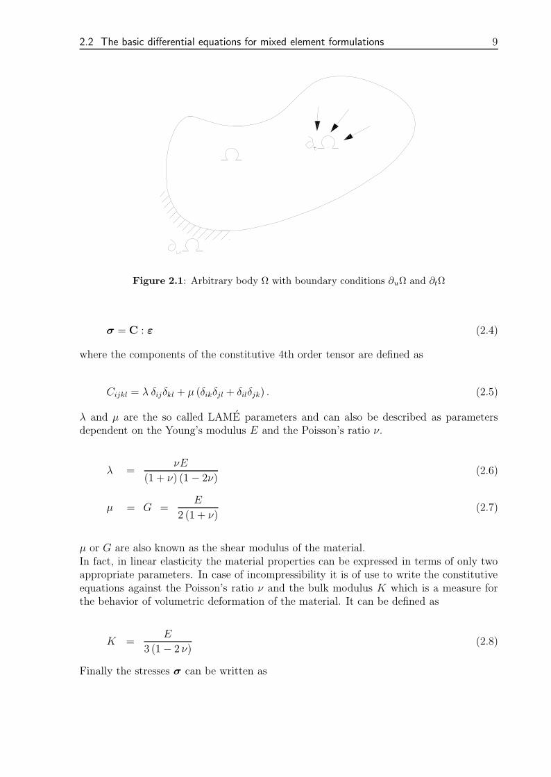
In many cases of calculations in solid mechanics the properties of the material of a body isleading to a incompressible behavior. For example some rubber like materials or materialsin an inelastic stadium can give an incompressible reply. In fact the compressibility canbe so small that it may be disregarded. In that case the material could be idealized ascompletely incompressible. The difficulty in the computation of incompressible mediumsis to predict the pressure. Whether it is possible to get adequate results for nearly incom-pressible materials using finite elements with only the displacements as free variables, thenumber of necessarily elements to get a default accuracy of the solution is much largerthan in case of problems with compressible properties.To display the difficulty of this problem we should consider an arbitrary body as in Fig.2.1.The material of the body is isotropic and will be described by the Young’s modulus Eand the Poisson’s ratio ν. The boundary-value problem for this continuously differentiablebody including the equilibrium conditions and the boundary conditions can be defined as
∇ · σ + f = 0 in Ω (2.1)
σ · n = t on ∂tΩ (2.2)
u = u on ∂uΩ (2.3)
where the surface of the body Ω is defined as ∂Ω = ∂uΩ ∪ ∂tΩ and ∂uΩ ∩ ∂tΩ = ∅.Additionally to the equilibrium and the boundary conditions we need the constitutiveequations which give the relation between the strains ε(u) as a function of the defor-mations u and the stresses σ. In linear elasticity we use the Hookean law in the formof
2.2 The basic differential equations for mixed element formulations 9
Figure 2.1: Arbitrary body Ω with boundary conditions ∂uΩ and ∂tΩ
σ = C : ε (2.4)
where the components of the constitutive 4th order tensor are defined as
Cijkl = λ δijδkl + µ (δikδjl + δilδjk) . (2.5)
λ and µ are the so called LAME parameters and can also be described as parametersdependent on the Young’s modulus E and the Poisson’s ratio ν.
λ =νE
(1 + ν) (1− 2ν)(2.6)
µ = G =E
2 (1 + ν)(2.7)
µ or G are also known as the shear modulus of the material.In fact, in linear elasticity the material properties can be expressed in terms of only twoappropriate parameters. In case of incompressibility it is of use to write the constitutiveequations against the Poisson’s ratio ν and the bulk modulus K which is a measure forthe behavior of volumetric deformation of the material. It can be defined as
K =E
3 (1− 2 ν)(2.8)
Finally the stresses σ can be written as
10 CHAPTER 2: THE MIXED FINITE ELEMENT FORMULATION
σ = Kεv1 + 2µ dev(ε) (2.9)
Thereby is
εv = ∇ · u (2.10)
the volumetric strain, the matrix 1 the identity matrix and
dev(ε) = dev(∇su) (2.11)
the deviatoric strains.As ν approaches 0.5, resistance to volume change is greatly increased assuming resistanceto shearing remains constant. This may be seen by calculating the ratio of the bulkmodulus to the shear modulus.
K
µ=
2 (1 + ν)
3 (1− 2 ν)(2.12)
Clearly, as ν → 0.5, the ratio approaches infinity. The limiting value ν = 0.5 thus rep-resents incompressibility. This limit creates problems in the equations of the constitutivelaw (2.9). A possible formulation to circumvent this problem can be written consideringthe hydrostatic pressure p as an independent unknown additionally to the displacementfield u. The pressure p in the body is defined as
p = −Kεv = −1
3σv (2.13)
with σv as the volumetric stresses. In case of ν = 0.5, K is going to infinity and εv isgetting zero. The pressure of course has nevertheless a finite value. With regard to thisthe stress tensor can be expressed such as
σ = −p 1 + 2µ dev(∇su) (2.14)
where the displacements u and additionally the pressure p are the two unknown variables.With the definition of the pressure in (2.13) we now get a new condition which has to befulfilled at all times.
p
K+ εv =
p
K+∇ · u = 0 (2.15)
In case of incompressibility (K →∞) the condition changes into
2.3 The variational formulation for mixed finite elements 11
∇ · u = 0 (2.16)
Now we can summarize the considerations to the following set of differential equations:
∇ · σ + f = 0 in Ω (2.17)p
K+∇ · u = 0 in Ω (2.18)
σ · n = t on ∂tΩ (2.19)
u = u on ∂uΩ (2.20)
wherein the components of the stress tensor are now a function of the displacements uand the pressure p (2.14).
2.3 The variational formulation for mixed finite ele-
ments
The previous considerations point to significant difficulties which appear if we use finiteelements applying only to displacements in case of incompressible media. The very smallvolumetric strain, so called dilatation, which approach to zero if exists complete incom-pressibility, will be dominated by the derivations of the displacements. This derivationscan not be predicted as accurate as the displacements themselves. And every imprecisionin the volumetric strains will appear also as an error in the stresses. Finally this erroron his part will influence the forecasting of the displacements because the external forcesare balanced by the stresses via the principal of the virtual work. Although solutions arepossible it could be necessary to use a very fine discretization of finite elements to get anappropriate solution.With regard to this aspect it would be useful to develop a finite element formulation that,independently of the Poisson’s ratio, gives accurate solutions even if ν is nearly 0.5. Thisleads to a formulation in which the deformations and the stresses can be defined indepen-dently of the bulk modulus. Finite element formulations which show this special propertycould also be called as (volumetric) locking-free elements. The locking of elements has theeffect that the value of the computed displacements are much smaller than the expecteddisplacements which should appear. Whether the normal displacement-related formula-tion locks in case of nearly incompressibility, it is as well an important aspect that alsothe stresses and the pressure respectively are very imprecise. Effective elements whichneglect the locking behavior in nearly incompressible problems can be deduced from theinterpolation of the displacement and additionally the pressure as done in the previoussection.
12 CHAPTER 2: THE MIXED FINITE ELEMENT FORMULATION
2.3.1 The weak form
The variational or weak counterpart could be deduced directly from the strong formulationof the previous chapter (2.17)-(2.18). However, it is necessary to define at first the rightspaces of the used functions which can solve the given problem.
L2(Ω) =
v |
∫
Ω
v2 dΩ <∞
(2.21)
H1(Ω) =
v ∈ L2(Ω) |∂v
∂xj∈ L2(Ω) , j = 1, . . . , ndim
(2.22)
The space L2 is the space of the quadratic integrable functions in the considered volumeand H1 the so called Hilbert-space, in which the functions v and its derivatives areelements of the space L2.To write the variational formulation in dependency of the variables u and p the stressshould be defined as in Eq.(2.14). After specified multiplication with the variations of thedisplacements and the pressure the following abstract formulation can be obtained
a(u,v) + b(p,v) = l(v) ∀ v ∈ V (2.23)
b(q,u) = 0 ∀ q ∈ Q (2.24)
where
a(u,v) = 2µ
∫
Ω
∇sv : ∇su dΩ (2.25)
b(p,v) =
∫
Ω
p∇ · v dΩ (2.26)
b(q,u) =
∫
Ω
q(∇ · u−1
Kp) dΩ (2.27)
l(v) = (v, f) + (v, t)∂tΩ =
∫
Ω
v · f dΩ +
∫
∂tΩ
v · t dΓ (2.28)
and the spaces
V =v ∈ H1(Ω) | v = 0 , in ∂uΩ
(2.29)
Q = L2(Ω) (2.30)
Finally the discretized formulation of the weak form can be deduced by choosing theinterpolation functions for the displacements, the pressure and their variations for everyelement in the way that the spaces comply with Vh ⊂ V and Qh ⊂ Q. Referring to thisEqs.(2.23) and (2.24) can be rewritten as
2.3 The variational formulation for mixed finite elements 13
a(uh,vh) + b(ph,vh) = l(vh) ∀ vh ∈ Vh (2.31)
b(qh,uh) = 0 ∀ qh ∈ Qh (2.32)
The approximation of the displacement field and its variations can be defined as
uh|Ωe = Nue , vh|Ωe = Nve (2.33)
where
N = [NA NB, . . . NNN ]T , NA = NA 1ND , with A = 1, . . . , NN (2.34)
are the interpolation functions and
ue = [uA uB ... uNN ]T , ve = [vA vB ... vNN ]T (2.35)
the displacements at the respective nodes. Each vector is subdivided into the number ofdimensions uA = uA
1 ... uAND and respectively vA = vA
1 ... vAND. The same scheme can
also be applied on the pressure field and its variation
ph|Ωe = Np pe , qh|Ωe = Np qe (2.36)
with
Np = [NAp NB
p . . . NNNp ]T (2.37)
and
pe = [pA pB . . . pNN ]T , qe = [qA qB . . . qNN ]T (2.38)
2.3.2 The matrix formulation
If we now insert the deduced relations into the weak form in Eqs. (2.23) and (2.24) andmake use of the Lemma for variational calculations (that the formulations holds for anyarbitrary variation v and q) we get the elementwise linear equation system
[Kuu Kup
Kpu Kpp
]e [up
]e
=
[R0
]e
(2.39)
14 CHAPTER 2: THE MIXED FINITE ELEMENT FORMULATION
with
Keuu =
∫
Ωe
(BA)T DBB dΩ (2.40)
Keuu is the element stiffness matrix which connects the displacements, in form of BA and
BB as the differential operators of the shape functions, with the deviatoric part of theconstitution matrix D.
Keup = (KT
pu)e =
∫
Ωe
bA NBp dΩ , with bA =
[NA
,1 . . . NA,ND
]T(2.41)
are mixed terms depending on the displacements as well as on the pressure and finally
Kepp = −
∫
Ωe
(NAp )T NB
p dΩ (2.42)
is a term which depends only on the pressure. After assembling the element matrices wecome to the global formulation
[Kuu Kup
Kpu Kpp
] [up
]
=
[R0
]
(2.43)
These are now the basic equations for the formulation of finite elements with the dis-placements and the pressure as unknown variables. If incompressibility exists the termdepending only on the pressure Kpp will be dropped and the linear equation systemchanges into
[Kuu Kup
Kpu 0
] [up
]
=
[R0
]
(2.44)
where we can see that the second equation only contains the displacements as un-knowns. This is generally important for particular formulations like the discontinuousu/p-formulation, mentioned before (see chapter 2). After the derivation of the basicequations for displacement/pressure-based elements the main problem is now to find ef-fective interpolation functions for the displacements and the pressure so that accuratesolutions are obtained. If the ratio of the interpolation functions of the pressure to thedisplacements is too high, the element can behave like a displacement-based element thatwould be very inaccurate. On the other hand if the ratio is too low, the inaccuracyappears in the solution of the pressure which could be of a higher order.
2.4 Illustration of a fundamental difficulty 15
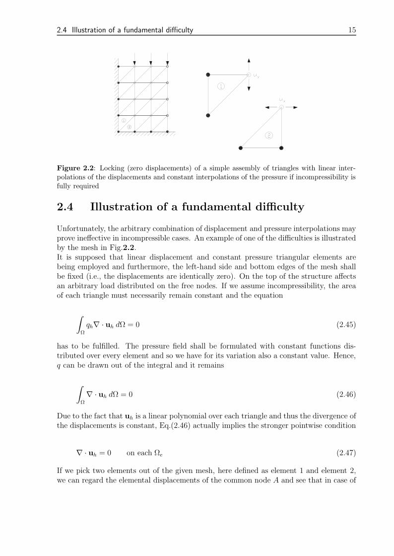
Figure 2.2: Locking (zero displacements) of a simple assembly of triangles with linear inter-polations of the displacements and constant interpolations of the pressure if incompressibility isfully required
2.4 Illustration of a fundamental difficulty
Unfortunately, the arbitrary combination of displacement and pressure interpolations mayprove ineffective in incompressible cases. An example of one of the difficulties is illustratedby the mesh in Fig.2.2.It is supposed that linear displacement and constant pressure triangular elements arebeing employed and furthermore, the left-hand side and bottom edges of the mesh shallbe fixed (i.e., the displacements are identically zero). On the top of the structure affectsan arbitrary load distributed on the free nodes. If we assume incompressibility, the areaof each triangle must necessarily remain constant and the equation
∫
Ω
qh∇ · uh dΩ = 0 (2.45)
has to be fulfilled. The pressure field shall be formulated with constant functions dis-tributed over every element and so we have for its variation also a constant value. Hence,q can be drawn out of the integral and it remains
∫
Ω
∇ · uh dΩ = 0 (2.46)
Due to the fact that uh is a linear polynomial over each triangle and thus the divergence ofthe displacements is constant, Eq.(2.46) actually implies the stronger pointwise condition
∇ · uh = 0 on each Ωe (2.47)
If we pick two elements out of the given mesh, here defined as element 1 and element 2,we can regard the elemental displacements of the common node A and see that in case of

16 CHAPTER 2: THE MIXED FINITE ELEMENT FORMULATION
incompressibility (the Area of every element may not increase) both elements could onlyachieve contrary displacements. This leads to the fact that the displacement has to bezero in this node if the elements shall remain compatible. Identical reasoning may be usedto conclude that every node in the entire mesh must have zero displacement. Thus theonly possible incompressible displacement is uh = 0. This result is preserved, no matterhow many elements are present in each direction. Clearly, this type of mesh offers noapproximation power whatsoever and is a simple device for the mesh locking. It is butone of the difficulties afflicting problems of incompressibility.In the nearly incompressible case, the same phenomenon occurs, only this time uh
∼= 0.Thus introducing slight compressibility does not solve the problem. For these kinds ofproblems a mathematical convergence theory for mixed finite element methods of thetype under consideration has been established by some authors and is known as theLadyzhenskaya-Babuska-Brezzi condition (LBB). To establish whether or not this condi-tion is satisfied for elements of interest is not so simple. Hence, the next chapter givesattention to some previous properties of finite element solutions and then comes to a shortexplanation of the LBB-condition.
2.5 The Mixed Patch Test
2.5.1 Important properties of finite element solutions
To understand the necessity of specific conditions, mixed finite element methods has tofulfill, it is helpful to look primarily at some important properties of basic finite elementmethods. The problem of elasticity can be written as
Find u ∈ V, such that :
a(u,v) = (f ,v) ∀ v ∈ V (2.48)
whereas the vector space V is defined as
V =
v |v ∈ L2(Ω) |∂vi
∂xj
∈ L2(Ω) , with: i, j = 1, 2, 3 | v = 0 on ∂uΩ
(2.49)
Here is
L2(Ω) =
w |
∫
Ω
(3∑
i=1
(wi)2
)
dΩ = ‖w‖L2(Ω) <∞
(2.50)
the room of the quadratic integrable functions in the considered volume. Thus (2.49)defines a general three dimensional function space whereas the functions disappear onthe edge of the body and the squares of the functions as well as its first derivatives areintegrable. Accordingly to V we can define a kind of energy norm
2.5 The Mixed Patch Test 17
‖v‖2E = a(v,v) (2.51)
This norm describes the double of the strain energy which contains a body if it is exposedto the displacement field v. Assumed that the body is bedded in the right way, the norm‖v‖2E is bigger than zero for all v 6= 0. Additionally we have to define the so calledSobolev-norms of the order s = 0 and s = 1.
s = 0 :
(‖v‖0)2 =
∫
Ω
(3∑
i=1
(vi)2
)
dΩ (2.52)
s = 0 :
(‖v‖1)2 = (‖v‖0)
2 =
∫
Ω
[3∑
i,j=1
(∂vi
∂xj
)2]
dΩ (2.53)
Hence we get the following properties of the bilinear form a(·, ·)
∃M > 0 so, that ∀ v1,v2 ∈ V, |a(v1,v2)| ≤ M‖v1‖1‖v2‖1 (2.54)
∃ α > 0 so, that ∀ v ∈ V, a(v,v) ≥ α(‖v1‖1)2 (2.55)
whereas (2.54) is the property of the continuity of the bilinear form a(·, ·) and (2.55)the ellipticity or coercivity. Thereby the constants α and M depend on the actuallyconsidered elastic problem including the material parameters but they are independentof the displacement field v. These two properties of continuity and ellipticity are fulfilledif feasible norms are used, like in this case the Sobolev-norm of the order one, and if weassume a stable bearing of the structure. The mathematic device of this assumptions areexplained in [6]. On this two properties bases the inequation
c1‖v‖1 ≤ [a(v,v)]1/2 ≤ c2‖v‖1 (2.56)
with the two constants c1 and c2 independent of v. From this inequality we can nowrewrite the known convergence criteria
a(u− uh,u− uh)→ 0 as h→ 0 (2.57)
in the form
‖u− uh‖1 → 0 as h→ 0 (2.58)
18 CHAPTER 2: THE MIXED FINITE ELEMENT FORMULATION
whereas h specifies the size of the used elements. This shows that the energy norm bysolving of problems converges with the same order like the Sobolev-1-norm.These conclusions in case of elasticity problems contains an important aspect that thedefinite solution to the problem has to come up to a finite strain energy (Eqs. (2.56) and(2.57)). A must for the definite solution is also its uniqueness. If for example u1 and u2
shall be two various solutions of a problem, then
a(u1,v) = (f ,v) ∀ v ∈ V (2.59)
and as well
a(u2,v) = (f ,v) ∀ v ∈ V (2.60)
The subtraction leads to
a(u1 − u2,v) = 0 ∀ v ∈ V (2.61)
Appointing in particular
v = u1 − u2 (2.62)
leads to
a(u1 − u2,u1 − u2) = 0 (2.63)
and with regard to (2.56) we get
‖u1 − u2‖1 = 0 (2.64)
which is the same as u1 ≡ u2. For this reason there is no possibility for two varioussolutions.Now we define Vh as a space of finite element displacement functions and vh shall be anarbitrary element of this space which can be extracted of the displacement interpolations.Additionally uh is the finite element solution and therewith an element of Vh, too. Thenthe finite element solution of this problem can be written as
Finduh ∈ Vh, such that :
a(uh,vh) = (f ,vh) ∀ vh ∈ Vh (2.65)
The space is again defined as
2.5 The Mixed Patch Test 19
Vh =
vh |vh ∈ L2(Ω) |∂(vh)i
∂xj
∈ L2(Ω) , i, j = 1, 2, 3 | vh = 0 on ∂uΩ
(2.66)
and it is obvious that Vh ⊂ V.The relation (2.65) is the principle of virtual forces for the to Vh corresponding finiteelement discretization. According to this solution space the conditions of the continuity(2.54) and the ellipticity (2.55) are fulfilled by the use of vh ∈ Vh and we get for arbitraryVh a positive stiffness matrix. The relation between the finite element solution uh andthe discrete solution u of the problem is characterized by three important properties.The first property is
a(eh,vh) = 0 ∀ vh ∈ Vh (2.67)
where
eh = u− uh (2.68)
is the error between the discrete solution u and the finite element solution uh. This seemsevident if we know that the principle of virtual work implies that
a(u,vh) = (f ,vh) ∀ vh ∈ Vh (2.69)
and additionally
a(uh,vh) = (f ,vh) ∀ vh ∈ Vh (2.70)
Because if we subtract these two equations we come finally to Eq.(2.68). So it can be saidthat the error eh is orthogonal in a(·, ·) to all vh in Vh and by increasing the space Vh,whereas Vh ⊂ V still holds, the accuracy of the solution increases, too.From this first property can be derivated two other properties. Thus the second propertystates that
a(uh,uh) ≤ a(u,u) (2.71)
This can be proved by
a(u,u) = a(uh + eh,uh + eh)
= a(uh,uh) + 2a(uh, eh) + a(eh, eh) (2.72)
= a(uh,uh) + a(eh, eh)
20 CHAPTER 2: THE MIXED FINITE ELEMENT FORMULATION
where uh is used in case of vh. For every error eh 6= 0, we get a(eh, eh) > 0 if we assumethat ‖v‖E ≥ 0. That means that strain energy obtained by the finite element solution isalways smaller or equal the strain energy obtained by the discrete solution.The third property states that
a(eh, eh) ≤ a(u− vh,u− vh) ∀ vh ∈ Vh (2.73)
As proof it can be used the Eq.(2.72) to get for an arbitrary wh ∈ Vh
a(eh + wh, eh + wh) = a(eh, eh) + a(wh,wh) (2.74)
And from this
a(eh, eh) ≤ a(eh + wh, eh + wh) (2.75)
With defining wh = uh − vh we come to the statement in (2.73).The third property signifies that the finite element solution uh is chosen from all possibledisplacement functions vh ∈ Vh in this way that the strain energy, corresponding tothe difference between the discrete and the finite element displacement u − uh, gets aminimum.Moreover we get by using Eq.(2.73) as well as the ellipticity (2.55) and the continuity(2.54) of the bilinear form
α‖u− uh‖21 ≤ a(u− uh,u− uh)
= infvh∈Vh
a(u− vh,u− vh) (2.76)
≤ M infvh∈Vh
‖u− vh‖1 ‖u− vh‖1
with inf as the Infimum, i.e. the lower limit. Let
d(u,Vh) = limh→0
infvh∈Vh
‖u− vh‖ (2.77)
be the minimal distance between the discrete and the finite element solution if the elementsize goes to zero, then we come to the property
‖u− uh‖ ≤ cd(u,Vh) (2.78)
where c =√
M/α is a constant which does not depend on the element size h but on thematerial properties. This inequality is also called the Lemma of Cea [6].These three derived properties give a valuable insight in which way the finite element
2.5 The Mixed Patch Test 21
solutions has to be chosen from the possible displacement functions in a given finiteelement mesh. The inequality (2.78) which is based on the property (2.73) means that itis a sufficient condition of convergence if limh→0 inf ‖u− vh‖1 = 0 holds for any arbitraryu ∈ V. Furthermore from the second and the third property it can be deduced that forthe finite element solution the error of the strain energy within the possible pattern ofdisplacements in a given mesh is minimized and that the finite element dependent strainenergy approaches from below to the discrete strain energy if increasingly finer meshesare used.After these considerations to the properties of the finite element solutions, it is now easierto follow the next section in which the mathematical requirements for mixed finite elementformulations shall be introduced.
2.5.2 The basic requirements for mixed finite elements
As seen in the previous derivation of the mixed finite element method, to prevent the useof inefficient elements it is necessary to find adequate conditions for the solutions of theproblem which should be independent of the material parameters in order to avoid theinfluence of incompressibility where K →∞. In case of mathematical aspect we search acondition for the space Vh so, that
‖u− uh‖ ≤ cd(u,Vh) (2.79)
whereas c now should be a constant independent of the element size h and the materialparameters, particularly the bulk modulus K. The distance d(u,Vh) shall be defined as
d(u,Vh) = infvh∈Vh
‖u− Vh‖ = ‖u− uh‖ (2.80)
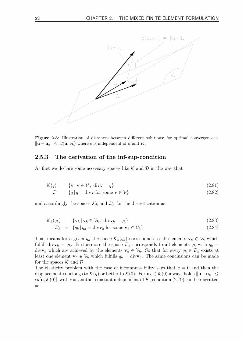
where uh is an element in Vh but not necessarily the finite element solution. For the betterunderstanding what is the meaning of this distance the Fig.2.3 shall give a possible idea.The inequation (2.79) means that the difference between the discrete solution u and thefinite element solution uh will be smaller than a reasonable measured constant c timesd(u,Vh). In condition (2.78) we came to the same conclusion except for the independenceof the material parameters in terms of the bulk modulus K. If condition (2.79) is fulfilledwith a reasonable measured constant c it is said that the accuracy of the finite elementsolution will increase independently of the bulk modulus K if the element size h will bedecreased and the finite element discretization is getting reliable. So the condition (2.79)is the basic requirement for the general finite element discretization to get non-lockingelement formulations. The condition in (2.79) seems very general and it is difficult to showit for any element formulation. Therefore it shall be an aim to rewrite this condition in amuch practical manner what will lead to the so called inf-sup-condition.
22 CHAPTER 2: THE MIXED FINITE ELEMENT FORMULATION
Figure 2.3: Illustration of distances between different solutions; for optimal convergence is‖u− uh‖ ≤ cd(u,Vh) where c is independent of h and K.
2.5.3 The derivation of the inf-sup-condition
At first we declare some necessary spaces like K and D in the way that
K(q) = v |v ∈ V , divv = q (2.81)
D = q | q = divv for some v ∈ V (2.82)
and accordingly the spaces Kh and Dh for the discretization as
Kh(qh) = vh |vh ∈ Vh , divvh = qh (2.83)
Dh = qh | qh = divvh for some vh ∈ Vh (2.84)
That means for a given qh the space Kh(qh) corresponds to all elements vh ∈ Vh whichfulfill divvh = qh. Furthermore the space Dh corresponds to all elements qh with qh =divvh which are achieved by the elements vh ∈ Vh. So that for every qh ∈ Dh exists atleast one element vh ∈ Vh which fulfills qh = divvh. The same conclusions can be madefor the spaces K and D.The elasticity problem with the case of incompressibility says that q = 0 and then thedisplacement u belongs to K(q) or better to K(0). For uh ∈ K(0) always holds ‖u−uh‖ ≤cd[u,K(0)], with c as another constant independent of K, condition (2.79) can be rewrittenas
2.5 The Mixed Patch Test 23
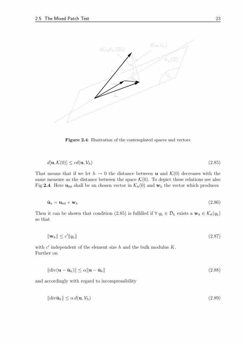
Figure 2.4: Illustration of the contemplated spaces and vectors
d[u,K(0)] ≤ cd(u,Vh) (2.85)
That means that if we let h → 0 the distance between u and K(0) decreases with thesame measure as the distance between the space K(0). To depict these relations see alsoFig.2.4. Here uh0 shall be an chosen vector in Kh(0) and wh the vector which produces
uh = uh0 + wh (2.86)
Then it can be shown that condition (2.85) is fulfilled if ∀ qh ∈ Dh exists a wh ∈ Kh(qh)so that
‖wh‖ ≤ c′‖qh‖ (2.87)
with c′ independent of the element size h and the bulk modulus K.Further on
‖div(u− uh)‖ ≤ α‖u− uh‖ (2.88)
and accordingly with regard to incompressibility
‖divuh‖ ≤ α d(u,Vh) (2.89)
24 CHAPTER 2: THE MIXED FINITE ELEMENT FORMULATION
It is also obvious the
‖u− uh0‖ = ‖u− uh + wh‖
≤ ‖u− uh‖+ ‖wh‖ (2.90)
Now it shall be assumed that condition (2.87) holds for qh = divuh. For the reason thatdivuh0 = 0 and with respect to Eq.(2.80) we get
‖u− uh0‖ ≤ d(u,Vh) + c′‖qh‖
= d(u,Vh) + c′‖divuh‖ (2.91)
≤ d(u,Vh) + c′α d(u,Vh) (2.92)
Due to the fact that uh0 ∈ Kh(0) we can finally write
d[u,Kh(0)] ≤ ‖u− uh0‖ ≤ (1 + αc′) d(u,Vh) (2.93)
This condition corresponds to (2.85) for c = 1 + αc′ and we see that c is independent ofthe element size h and the bulk modulus K. The result shows that condition (2.85) canbe deviced by using only the inequation (2.87) and this inequation therefore is the basicrequirement to get a finite element formulation with an ideal rate of convergence.With the variables qh and wh ∈ Kh(qh) condition (2.87) can be deduced as
‖wh‖ ‖qh‖ ≤ c′‖qh‖2 = c′
∫
Ω
qh div wh dΩ (2.94)
or as the condition that for all qh ∈ Dh exists such a wh ∈ Kh(qh) that
1
c′‖qh‖ ≤
∫
Ωqh div wh dΩ
‖wh‖(2.95)
Thus it shall be
1
c′‖qh‖ ≤ sup
vh∈Vh
∫
Ωqh div vh dΩ
‖vh‖(2.96)
and from this we come to the condition
infqh∈Dh
supvh∈Vh
∫
Ωqh div vh dΩ
‖vh‖‖qh‖≥ β > 0 (2.97)
2.5 The Mixed Patch Test 25
with β = 1/c′ as a constant independent of h and K. This so called inf-sup-conditionor LBB-condition states that for an effective finite element discretization there has tobe for any arbitrary qh ∈ Dh such a vh ∈ Vh that the quotient in (2.97) is bigger orequal β and bigger than 0 and if this condition is passed the discretization possesses theapproximation criteria that (2.85) will be fulfilled. After all the goal is now to develop anefficient mixed element formulation which even pass the LBB-condition to be sure thatthe formulation is adequate for quality of the finite element solutions. For elements thatsatisfy the LBB-condition, error estimates of the following form
‖uh − u‖1 + ‖ph − p‖0 = O(hmin[k,l+1]) (2.98)
may be established. Where k and l are the orders of the displacement and pressureinterpolations, respectively. If k = min[k, l + 1] the rate of convergence is said to beoptimal. Clearly, elements that satisfy the LBB-condition will not lock. But to establishwhether or not this condition is satisfied for elements of interest is not a trivial taskbecause the formulation of the condition to be fulfilled has a very mathematical characterand can not be applied easily nether on every finite element formulation nor on arbitrarymesh geometries. Thus it is desirable to have a simple procedure of constraint countingproves quite effective, see also [16].
2.5.4 Constraint counts
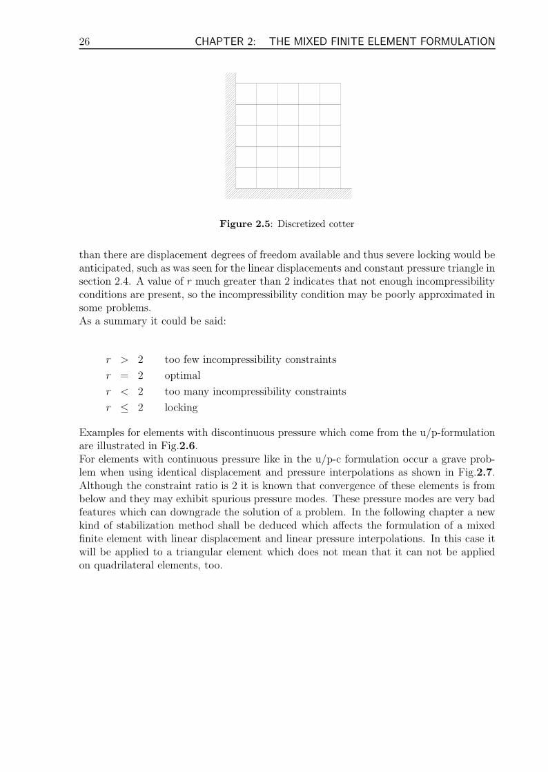
The constraint counts method is a heuristic approach for determining the ability of an el-ement to perform well in incompressible and nearly incompressible applications. It shouldbe emphasized that this is not a precise mathematical method for assessing elements butrather a quick and simple tool for obtaining an indication of element potential. However,it does seem to be able to predict a propensity for locking. There are, of course, otherissues that need to be considered in an overall evaluation of element performance. Topicture this method very intelligible it should be demonstrated with a simple exampleillustrated in Fig.2.5. Here neq shall represent the total number of displacement equa-tions after boundary conditions have been imposed and nc represents the total number ofincompressibility constraints. As long as the pressure equations are linearly independent,nc will be equal to the number of pressure equations neq. Additionally it shall be definedthe so called constrained ration r by
r =neq
nc(2.99)
Now the interest lies in values of r as nes, the number of elements per side approachesinfinity. The conjecture is that r should mimic the behavior of the number of equilibriumequations divided by the number of incompressibility conditions for the governing systemof partial differential equations. These are the number of space dimensions nsd and 1,respectively. So in two dimensions, the ideal value of r would be 2. A value of r less than2 would indicate a tendency to lock. If r ≤ 1, there are more constraints of the pressure
26 CHAPTER 2: THE MIXED FINITE ELEMENT FORMULATION
Figure 2.5: Discretized cotter
than there are displacement degrees of freedom available and thus severe locking would beanticipated, such as was seen for the linear displacements and constant pressure triangle insection 2.4. A value of r much greater than 2 indicates that not enough incompressibilityconditions are present, so the incompressibility condition may be poorly approximated insome problems.As a summary it could be said:
r > 2 too few incompressibility constraints
r = 2 optimal
r < 2 too many incompressibility constraints
r ≤ 2 locking
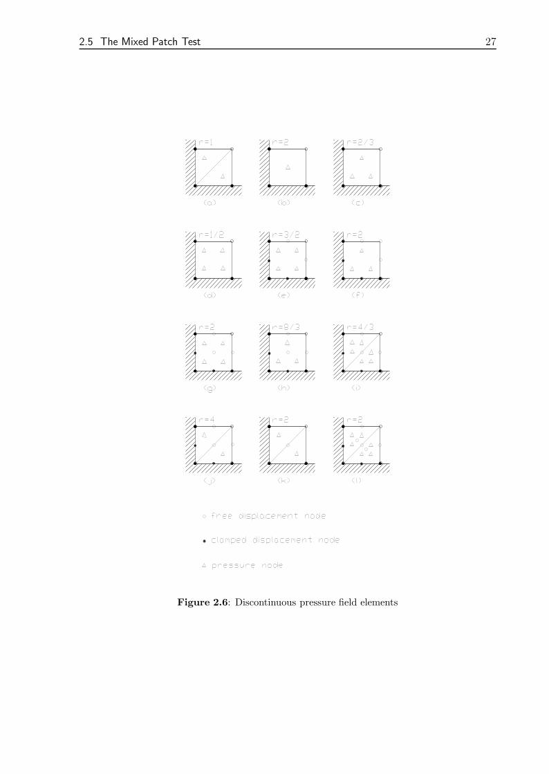
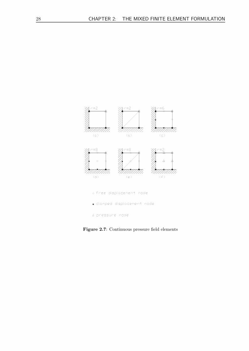
Examples for elements with discontinuous pressure which come from the u/p-formulationare illustrated in Fig.2.6.For elements with continuous pressure like in the u/p-c formulation occur a grave prob-lem when using identical displacement and pressure interpolations as shown in Fig.2.7.Although the constraint ratio is 2 it is known that convergence of these elements is frombelow and they may exhibit spurious pressure modes. These pressure modes are very badfeatures which can downgrade the solution of a problem. In the following chapter a newkind of stabilization method shall be deduced which affects the formulation of a mixedfinite element with linear displacement and linear pressure interpolations. In this case itwill be applied to a triangular element which does not mean that it can not be appliedon quadrilateral elements, too.
2.5 The Mixed Patch Test 27
Figure 2.6: Discontinuous pressure field elements
28 CHAPTER 2: THE MIXED FINITE ELEMENT FORMULATION
Figure 2.7: Continuous pressure field elements
Chapter 3
A Stabilized Mixed ElementFormulation
3.1 Introduction
In this chapter a formulation of triangular and tetrahedral elements shall be developedwith linear interpolation functions for the displacements and the pressure field with regardto small deformations. As we have seen in the previous chapter, the possibility to usea linear/linear formulation requires a kind of stabilization method for the element tocircumvent the Ladyzhenskaya-Babuska-Brezzi condition. The stabilization techniquewhich shall be used in this work will be deduced from the orthogonal sub-grid scalesapproach. It should be pronounced that this kind of stabilization method can also beapplied to elements of higher order and different geometries.
3.2 The sub-grid-scale approach
The solution of a problem for finite element methods consists in searching in the spaceof functions with finite dimension Vh ⊂ V an approximation to the solution which hasa required accuracy. The basic idea of the sub-grid scale approach is to consider thatthe continuous displacement field can be split in two components, one coarse and a finerone, corresponding to different scales or levels of resolution. The solution of the con-tinuous problem contains components from both scales. For the solution of the discreteproblem to be stable, it is necessary to, somehow, include the effect of both scales in theapproximation. The coarse scale can be appropriately solved by a standard finite elementinterpolation, which however can not solve the finer scale. Nevertheless, the effect of thisfiner scale can be included, at least locally, to enhance the stability of the pressure inthe mixed formulation. But at first this method shall be applied only on the displace-ment formulation to present it rather clearly. Afterward it will be enhanced on the mixedformulation.
29
30 CHAPTER 3: A STABILIZED MIXED ELEMENT FORMULATION
3.2.1 The basic idea
The problem which has been already defined in the previous chapter was:
Find the displacement field u : Ω→ RND so that, by given external forces t : ∂tΩ→ RND,body forces b : Ω → RND and also the displacements on the boundary ∂uΩ, followingequations are fulfilled:
∇ · σ + f = 0 in Ω (3.1)
σ · n = t on ∂tΩ (3.2)
u = u on ∂uΩ (3.3)
where the stresses σ at first only depends via the constitutive equation on the displace-ments u. To keep track of the derivation of the sub-scales, this problem shall be rewrittenin a more abstract form as:Find U ∈ V, with regard to the boundary conditions, so that
L (U) = F (3.4)
holds, where L(·) is the differential operator of this problem and F represents the forcevector
L(U) = −∇ · σ(U) (3.5)
F = f (3.6)
The variational formulation of this problem can be written as
∫
Ω
V · [F − L (U)] dΩ = 0 , ∀V ∈ V (3.7)
where the term∫
ΩV · L(U) includes derivations of second order of the displacements U.
With the aid of the partial integration the order can be compensated and we get
∫
Ω
V · L (U) dΩ = B (U,V)−
∫
∂tΩ
V · [σ (U) · n] dΓ (3.8)
in which the Green’s theorem is used in the first term of the right side B(U,V). Thevector n is the unit normal exterior to the integration domain and the term [σ(·) · n]stands for the tractions vector.After inserting this equation in (3.5) we come to
3.2 The sub-grid-scale approach 31
B(U,V) = L(V) , ∀V ∈ V (3.9)
with
L(V) =
∫
Ω
V · F dΩ +
∫
∂tΩ
V · [σ(U) · n] dΓ (3.10)
To apply the method of sub-grid scales, the displacements have to be enhanced by anadditionally displacement field in the way that
U = Uh + U (3.11)
As the solution of the finite elements is defined in the space referable to the finite elementsUh ∈ Vh, the enhanced displacements shall be defined in an equivalent space as U ∈ V ,the sub-grid scale. Considering the same result for the variations leads to
V = Vh + V (3.12)
where Vh ∈ Vh and U ∈ V. After this we come to the conclusion that the space of thedisplacement field U and its variation V can be composed by the two different spaces sowe get
V ' Vh ⊕ V (3.13)
It is reasonable to assume that the sub-grid displacements U will be sufficiently smallcompared to the finite element solution Uh. They can be viewed as a high-frequency
perturbation of the finite element field which cannot be resolved in the finite elementspace Vh. It can also be assumed that U and V vanish on the boundary ∂Ω.With this conclusions we can rewrite Eq. (3.9) and come to
B(Uh + U,Vh) = L(Vh) , ∀Vh ∈ Vh (3.14)
B(Uh + U, V) = L(V) , ∀ V ∈ V (3.15)
If the terms B(Uh + U,Vh) and B(Uh + U, V) are a linear function of the displacements,we can split these terms to get the following formulation
B(Uh,Vh) + B(U,Vh) = L(Vh) , ∀Vh ∈ Vh (3.16)
B(Uh, V) + B(U, V) = L(V) , ∀ V ∈ V (3.17)
32 CHAPTER 3: A STABILIZED MIXED ELEMENT FORMULATION
As we see, the first equation (3.14) is defined in the finite element scale and it solves thebalance of momentum including a term depending on the sub-grid scale which can be seenas a kind of stabilization term. The second equation (3.15) is formulated in the sub-gridscale and will be used to find an adequate definition for the enhanced displacement fieldU. That means, after evaluating the second equation, the solution for U can be utilizedto resolve the first equation. This is the essential idea of the proceeding, neverthelesssome important aspects of the application of the method of sub-grid scales have to beemphasized.To obtain a solution for the enhanced displacements U from Eq.(3.17) and use it inEq.(3.16), we have to accomplish some operations on element level which presupposesa notation for each element. As we define
∫
Ω′:=
∑NEe=1
∫
∂Ωe and∫
∂Ω′:=
∑NEe=1
∫
Ωe ,respectively, where NE is the number of elements of the finite element partition. Byusing once again the differential operator, Eq.(3.17) can be rewritten as
∫
Ω′
V · L(Uh) dΩ +
∫
Ω′
V · L(U) dΩ
+
∫
∂Ω′
V ·[
σ(Uh + U) · n]dΓ =
∫
Ω′
V · F dΩ ∀ V ∈ V (3.18)
Observe that σ(Uh + U) · n represents the exact tractions, assumed to be continuousacross interelement boundaries and thus the sum over these boundaries is zero. So wecome to the conclusion that
∫
Ω′
V ·[
L(
Uh + U)]
dΩ =
∫
Ω′
V · F dΩ , ∀ V ∈ V (3.19)
By means of the integration by parts, the second term of the left side in Eq.(3.16) can bedefined by
B(U,Vh) =
∫
Ω′
U · L∗(Vh) dΩ +
∫
∂Ω′
U · (σ(Vh) · n) dΓ (3.20)
where L∗ is the adjunct of the operator L. Now it can be made a simplification in definingthe sub-scales only in the interior of the element volume Ωe. That means that the integralover the boundary in (3.20) disappears. This is comparable to the method of adding abubble function to the element which values are zero at the boundary of the element likein the formulation of the MINI-element (see also [1], [17]).The operator L∗ can be calculated via the integration by parts with the following relationto L (without regard to the boundary)
∫
Ω
U · L∗(V) dΩ =
∫
Ω
V · L(U) dΩ (3.21)
Finally, Eq.(3.16) can be rewritten with the mentioned considerations as
3.2 The sub-grid-scale approach 33
B(Uh,Vh) +
∫
Ω′
U · L∗(Vh) dΩ = L(Vh) , ∀Vh ∈ Vh (3.22)
and Eq.(3.19) as
∫
Ω′
V · L(U) dΩ =
∫
Ω′
V · [F − L(Uh)] dΩ , ∀ V ∈ V (3.23)
The expression (3.23) is more or less the key point to capture the effects of the componentU used to enrich the standard finite element solution Uh. It relates the enhanced dis-placements U to the residuum Rh of the differential approximation for the finite elements,represented by Rh = F−L(Uh). Important is that it is not obliged to fulfill this equationpointwise, but only over the integral.Up to now, the presentation of the method of the sub-grid scales is general and the currentaim consists in obtaining a reliable approximation for U ∈ V at a moderate computa-tional effort. There already exist diverse possibilities to define the approximation of thesub-grid scales such as the definition of special functions for the enhanced displacementfield U in a manner similar to the enhanced assumed strain method (EAS). In principle,the finer enhanced space could be any complementary space to the finite element space.The method which is used in this work shall be developed in the next section and basedon considerations of R. Codina [8].
3.2.2 The orthogonal sub-scales
Codina proposed for the sub-grid scale as a reasonable possibility the orthogonal space tothe finite element space. This definition gives the origin for precise and clever formulationnamed as the method of orthogonal sub-scales. With regard to this method the space ofthe enhanced elements can be approximated as
V ≈ V⊥
h (3.24)
where V⊥h represents the orthogonal space of the finite element space Vh. Hence, the
enhanced elements U are now defined in this orthogonal space of Vh
U ∈ V⊥
h (3.25)
Then Eq. (3.23) comes to
∫
Ω′
V · L(U) dΩ =
∫
Ω′
V · [F − L(Uh)] dΩ , ∀ V ∈ V⊥
h (3.26)

34 CHAPTER 3: A STABILIZED MIXED ELEMENT FORMULATION
This equation represents the projection of the residuum of the differential equation Rh =F − L(Uh) on the orthogonal space of the finite element space V⊥
h . Even though withthis equation will not be found an exact value for the enhanced elements U, it is at leastpossible to approximate the linear operator L by a matrix of parameters like
L(U) ≈ τ−1e U (3.27)
If we additionally call Ph (·) the L2 orthogonal projection on the finite element space andP⊥
h (·) = (·) − Ph (·) the projection on the space V⊥h , orthogonal to the finite element
space, the enhanced elements U can be defined as
U = τ eP⊥
h ([F − L(Uh)]) in Ωe (3.28)
where τ e is the matrix of the stabilization parameters in each element. Codina devel-oped in the context of the equations of Oseen (see [9]) a deduction for the values of thestabilization parameters by means of a Fourier series expansion, based for the first timeon physical reasons. The values of the parameters of the matrix τ e depend on the coeffi-cients of the differential equation, as material or geometry parameters, and establish viathe comparison of the L2-norm of the residuum and the U over each element.
3.2.3 Aspects to the stabilization of the mixed formulation in
incompressibility
As we have seen in a previous chapter, the triangular and tetrahedral elements with thecombination of linear interpolations for the displacements and the pressure do not passthe LBB-condition (see chapter 2.5). However, with the aid of stabilization techniqueslike the method of orthogonal sub-scales, it is possible to circumvent the LBB-conditionand to present adequate results.To develop the method of orthogonal sub-scales for mixed formulations we start onceagain from Eq.(3.4) where
L(U) =
[−∇p− 2µ∇ · dev(∇su)
∇ · u− 1K
p
]
(3.29)
is the differential operator deduced from 2.2 and
F =
[f0
]
(3.30)
contains the volumetric forces. The vector U := [u p]T now contains the variables of themixed formulation, as well the displacements u ∈ V as the pressure p ∈ Q. The space to
3.2 The sub-grid-scale approach 35
which belongs U can be defined as W = V × Q. In the same manner, the terms of theweak form in (3.14) and (3.15) are
B(U,V) = a(u,v) + b(p,v) + b(q,u) (3.31)
L(V) = (f ,w) + (t,v)Γt(3.32)
with
a(u,v) = 2µ
∫
Ω
∇sv : ∇su dΩ (3.33)
b(p,v) =
∫
Ω
p∇ · v dΩ (3.34)
b(q,u) =
∫
Ω
q∇ · u dΩ (3.35)
With the use of the sub-grid scale approach the vector U = Uh + U is generally definedas
[up
]
︸ ︷︷ ︸
U
=
[uh
ph
]
︸ ︷︷ ︸
Uh
+
[up
]
︸ ︷︷ ︸
U
(3.36)
We see that there is also a possibility to enrich in addition to the displacements also thepressure by the sub-grid scales. But to circumvent the LBB-condition and as well toget adequate results for the solution, as we will see later on, it is not necessary to takeadditionally an enrichment of the pressure into account. What does not mean that itwould not be reasonable. The effects depending on the enrichment of the pressure fieldare not yet investigated and there could be the possibility that it improves once morethe results of the solution. However it should be obvious that the additional enrichmentof the pressure field leads to a higher cost of computing time. Thus a more intensiveinvestigation in this direction could be of a high value. The simplification of the methodin this work leads finally to the conclusion that the enhanced pressure part becomes p = 0.To reconsider the way of defining the stabilization matrix τ e we should refer once againto Codina. In [9] considerations were established to define the stabilization matrix τ e
in which the corresponding parameters were calculated in the scope of the problem ofOseen via the Fourier series expansion. In particular for the problem of Stoke’s flow [8]the matrix of the stabilization parameters (3.28) is defined as a diagonal matrix in theway that
τ e = τe
1. . .
1ND
0
(3.37)

36 CHAPTER 3: A STABILIZED MIXED ELEMENT FORMULATION
with
τe =ch2
2µ(3.38)
where h is the characteristic diameter of the mesh, µ the shear modulus and c a numer-ical constant that depends only on the element type. As a consequence of the previousconsiderations about the enrichment of the vector U, the last term of the diagonal matrixin (3.37) which stands for the pressure is zero.The definition of the stabilization parameter τe in (3.38) could also alter from the one ofCodina in [9]. There are as well other considerations to be found in the literature how todefine these stabilization parameters (see e.g. [11]). From the algorithmic point of viewτe is a robust parameter which is not affected as much by the value of the constant c if theconstant is defined in a reasonable order of magnitude. The numerical experiences haveshown that for linear elements the value of c is located in the dimension of 0.5 to 0.75.Having specified the manner of the stabilization, in the next section shall be deduced theformulation of stabilized mixed elements which is the main subject of this work.
3.3 Formulation in the elastic case
It can be proposed a mixed formulation of an elastic problem in which the incompressibilityrepresents the limitation of the general problem of compressibility. In this formulationwill be defined the pressure p as an independent variable additionally to the displacementsu.
3.3.1 Constitutive model
The constitutive comportment in infinite elasticity can be expressed by means of thefollowing couple of equations
σ = p1 + 2µ dev[∇su] (3.39)
p = Kεv with εv = ∇ · u (3.40)
where εv and dev[∇su] are the volumetric and deviatoric components of the deformations,respectively. K is the bulk modulus already defined in (2.8) and now rewritten in subjectto the LAME parameters as
K = λ +2
3µ (3.41)
As it can be observed from the constitutive equations (3.39) and (3.40), the decompo-sition of the deformations in their volumetric and deviatoric parts leads to a decoupled
3.3 Formulation in the elastic case 37
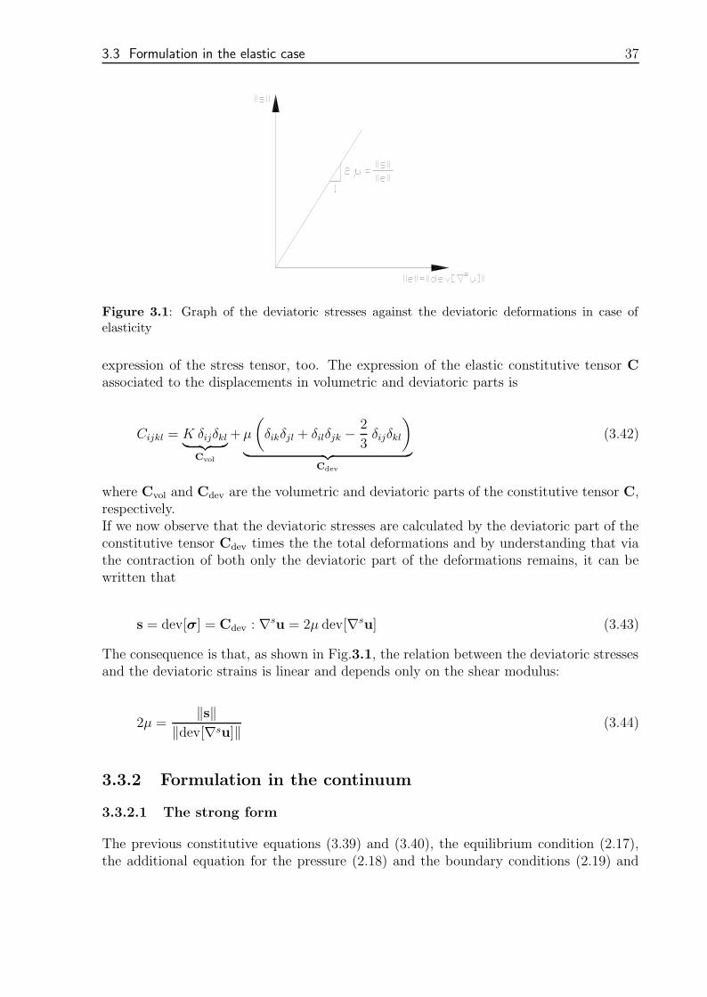
Figure 3.1: Graph of the deviatoric stresses against the deviatoric deformations in case ofelasticity
expression of the stress tensor, too. The expression of the elastic constitutive tensor Cassociated to the displacements in volumetric and deviatoric parts is
Cijkl = K δijδkl︸ ︷︷ ︸
Cvol
+ µ
(
δikδjl + δilδjk −2
3δijδkl
)
︸ ︷︷ ︸
Cdev
(3.42)
where Cvol and Cdev are the volumetric and deviatoric parts of the constitutive tensor C,respectively.If we now observe that the deviatoric stresses are calculated by the deviatoric part of theconstitutive tensor Cdev times the the total deformations and by understanding that viathe contraction of both only the deviatoric part of the deformations remains, it can bewritten that
s = dev[σ] = Cdev : ∇su = 2µ dev[∇su] (3.43)
The consequence is that, as shown in Fig.3.1, the relation between the deviatoric stressesand the deviatoric strains is linear and depends only on the shear modulus:
2µ =‖s‖
‖dev[∇su]‖(3.44)
3.3.2 Formulation in the continuum
3.3.2.1 The strong form
The previous constitutive equations (3.39) and (3.40), the equilibrium condition (2.17),the additional equation for the pressure (2.18) and the boundary conditions (2.19) and
38 CHAPTER 3: A STABILIZED MIXED ELEMENT FORMULATION
(2.20) define the problem of the strong form. Following the abstract nomenclature of thechapter 3.2, the linear elastic problem can be expressed as:Given are the prescribed values of the external forces t : ∂tΩ→ RND, the displacementson the boundary ∂uΩ and the body forces b : Ω → RND; find then U := [u, p]T ∈ W =V × Q, so that
L(U) = F (3.45)
where
L(U) =
[−∇p− 2µ∇ · dev(∇su)
∇ · u− 1K
p
]
(3.46)
F =
[f0
]
(3.47)
together with the boundary conditions
u = 0 ∂uΩ (3.48)
σ · n = t ∂tΩ (3.49)
It is said that the equations of this formulation in the dominion are
∇p + 2µ∇ · dev[∇su] + b = 0 in Ω (3.50)
∇ · u−1
Kp = 0 in Ω (3.51)
where in the equilibrium condition (3.50) has changed the expression of the stresses σ
given as a function of u and p in case of the constitutive relation in (3.39).As we already mentioned, this formulation holds as well in case of compressibility as incase of incompressibility. And it is also obvious that for K →∞ the equation (3.51) hasto be changed into
∇ · u = 0 in Ω (3.52)
The adjunct L∗(·) of the differential operator L(·) in Eq.(3.46) can be calculated via theEq.(3.21). With the integration by parts this can be expressed as
L∗(V) =
[−∇p− 2µ∇ · dev(∇sv)
∇ · v− 1K
p
]
(3.53)
3.3 Formulation in the elastic case 39
3.3.2.2 The weak form
The variational or weak form of the problem is defined in that case as
Given are the prescribed values of the external forces t : ∂tΩ→ RND, the displacementson the boundary ∂uΩ and the body forces b : Ω → RND; find then U := [u, p]T ∈ W =V × Q, so that
B(U,V) = L(V) , ∀V ∈ W (3.54)
where V ∈ W is the vector of the variations of U and
B(U,V) := 〈∇sv, 2µ dev(∇su)〉+ 〈∇ · v, p〉+ 〈q,∇ · u〉 − 〈q,1
Kp〉 (3.55)
L(V) := 〈v,b〉+ 〈v, t〉∂t(3.56)
This weak formulation can be separated into a couple of two equations associated to thevariations of the displacements and the pressure, respectively
〈∇sv, 2µ dev(∇su)〉+ 〈∇ · v, p〉 = l(v) , ∀ v ∈ V0 (3.57)
〈q, (∇ · u−1
Kp)〉 = 0 , ∀ p ∈ Q (3.58)
where, as before, l(v) = 〈v,b〉+ 〈v, t〉∂tΩ is the term of the external forces. This pair ofequations can be expressed as well in a vector notation like
R(U,V) = 0 ∀ V ∈ V0 (3.59)
where
R(U,V) =
[〈∇sv, 2µ dev(∇su)〉 + 〈∇ · v, p〉 − l(v)
〈q, (∇ · u− 1K
p)〉
]
(3.60)
This notation is chosen because it permits more clearness for the upcoming deductions.The space in which exists U is defined as W = V × Q where V and Q are the spaces forthe displacements and the pressure, respectively
V =v |v ∈ H1(Ω) , v = 0 in ∂uΩ
(3.61)
Q =
q | q ∈ L2(Ω) ,
∫
Ω
q dΩ = 0
(3.62)
with

40 CHAPTER 3: A STABILIZED MIXED ELEMENT FORMULATION
L2(Ω) =
φ |
∫
Ω
φ2dΩ <∞
(3.63)
H1(Ω) =φ |φ ∈ L2(Ω) , φ′ ∈ L2(Ω)
(3.64)
The stabilization of this mixed formulation depends on the compliance of the LBB-condition. This condition leads to the necessity of using different interpolations for thedisplacement field u and the pressure field p in the finite element formulation. However,the already appointed stabilization technique of the sub-grid scale approach copes thecircumventing of the LBB-condition, although the same order of interpolations are usedfor the displacements and the pressure which shall be developed in the following section.
3.3.3 Extension on multiscales
As preassigned, the spaces of the finite element functions for u and p shall be chosen aslinear and continuous. So the spaces of the finite element approximations are defined asUh ∈ Wh = Vh ×Q ⊂ [H1(Ω)]ND+1.By using the method of orthogonal sub-grid scales (OSGS), proposed by R. Codina [8],whereupon the complementary space W is specified as the orthogonal space of the finiteelement space. Agreeing with this, we come to U ∈ W where we can approximateW ≈ W⊥
h . In the same way as in section 3.2.3, the refinement of the solution U = UhUis used to enrich the displacement field with the expectation to improve the stabilizationproperties of the mixed finite element formulation. Therefore we get for the vector ofunknowns
[up
]
=
[uh
ph
]
+
[u0
]
(3.65)
[vq
]
=
[vh
qh
]
+
[v0
]
(3.66)
where we disregard once again the enrichment of the pressure field. The continuumproblem transforms into:
Find Uh ∈ Wh and U ∈ W so that
B(Uh + U,Vh) = L(Vh) , ∀Vh ∈ Wh (3.67)∫
Ω′
V · L(Uh + U) dΩ =
∫
Ω′
V · F dΩ , ∀ V ∈ W (3.68)
which correspond respectively to the expressions (3.16) and (3.17) with regard to theidea formulated in Eq.3.2.1. The equation (3.67), defined in the finite element space,is equivalent to the couple of two equations with dependency to the variations of thedisplacements and the pressure, respectively
3.3 Formulation in the elastic case 41
〈∇svh, 2µ dev[∇s(uh + u)]〉Ω′ + 〈∇ · vh, ph〉Ω′ = l(vh) (3.69)
〈qh, (∇ · (uh + u)−1
Kp)〉Ω′ = 0 (3.70)
with l(vh) = 〈vh, f〉+ 〈vh, t〉∂tΩ. In the compact notation it can be written as
R(U,Vh) = 0 , ∀Vh ∈ Wh (3.71)
In (3.69) and (3.70) the gradient and the divergence are applied on (uh + u). Bothoperations are linear so that the term on the left side can be divided in two terms andthe equation can be rewritten as
R(U,Vh) = R(Uh,Vh) + R(U,Vh) = 0 , ∀Vh ∈ Wh (3.72)
where R(Uh,Vh) and R(U,Vh) are respectively
R(Uh,Vh) =
[〈∇svh, 2µ dev(∇suh)〉Ω′ + 〈∇ · vh, ph〉Ω′ − l(vh)
〈qh, (∇ · uh −1K
ph)〉Ω′
]
(3.73)
R(U,Vh) =
[〈∇svh, 2µ dev(∇su)〉Ω′
〈qh,∇ · u〉Ω′
]
(3.74)
The stabilization effect of the sub-scales appears in the terms contained in Eq.(3.74). Inthe same manner as in Eq.(3.22) the terms of (3.74) are evaluated via integration by parts.So we obtain an equivalent definition as in (3.74) but now expressed by the derivatives ofthe variations instead of the derivatives of u
R(U,Vh) =
[−〈u,∇ · [2µ dev(∇svh)]〉Ω′
−〈u,∇qh〉Ω′
]
(3.75)
In the same way the weak form in Eq.(3.68) can be put into a compact form so that weget
R(Uh + U, V) = 0 , ∀ V ∈ V0 (3.76)
with
R(Uh + U, V) =
[〈v,∇ · 2µ dev[∇s(uh + u)]〉Ω′ + 〈v,∇ph〉Ω′ + 〈v,b〉Ω′
0
]
(3.77)
42 CHAPTER 3: A STABILIZED MIXED ELEMENT FORMULATION
It can be observed that there is no associated equation to the variations of the pressurein the sub-grid scale space because we only have taken the displacements into account.After these expressions and by considering the linearity of the divergence in (3.77) we get
−〈v,∇ · [2µ dev(∇su)]〉Ω′ = 〈v,∇ph +∇ · 2µ dev(∇suh) + b〉Ω′ (3.78)
which is corresponding to Eq.(3.26). This expression connect, via the projection on theorthogonal space of the finite element space, the sub-scale u with the residuum of theequilibrium condition Rh = ∇ph +∇ · (2µ dev[∇suh]) + f . The sub-grid scale approachdeveloped in 3.2, expressed in Eq.(3.28), consists by taking into account that the sub-grid scale is proportional to the projection on the orthogonal space of the finite elementsolutions of the residuum of the equilibrium conditions. This proportionality is expressedin every element via the matrix of the stabilization parameters (3.37). In this case theapproximation results in
u = τeP⊥
h (∇ph +∇ · [2µ dev(∇suh)] + b) in Ωe (3.79)
where the stabilization parameter is defined as in Eq.(3.38). By using only elementswith linear interpolations, the second derivations of the finite element functions like ∇ ·(∇su) vanish. Furthermore it considers that the body forces b are approximated throughelements of the finite element space so that P⊥
h (b) = 0. Hence the sub-grid scale approachcan finally written as
u = τe[∇ph − Ph(∇ph)] (3.80)
where the orthogonal projection of a variable is calculated as P⊥h (·) = (·)− Ph(·), and (·)
is the identity of the variable.It is only missing to insert the obtained approximation for u into the equations corre-sponding to the finite element spaces (3.69) and (3.70). By taking into account that linearfunctions are used and by inserting the definition for the sub-grid scales u of (3.80) intoEq.(3.75) we get at last the stabilization term
R(U,Vh) =
[0
−∑nelm
e=1 τe〈∇qh · (∇ph −Πh)〉Ωe
]
(3.81)
with Πh = Ph(∇ph), the projection of the pressure gradient on the finite element spaceWh, which is defined as an additional nodal variable. This variable is calculated by theuse of the relation between the pressure gradient and its projection Πh in the way that
〈∇ph, ηh〉 = 〈Πh, ηh〉 , ∀ ηh ∈ Vh (3.82)
3.3 Formulation in the elastic case 43
Finally, as a result of the developed proceeding, the proposed stabilized formulation totreat the elastic problem via linear triangular or tetrahedral elements is:
〈∇svh, 2µ dev(∇suh)〉+ 〈∇ · vh, ph〉 − l(vh) = 0 , ∀ vh ∈ Vh (3.83)
〈qh,∇ · uh −1
Kph〉 −
nelm∑
e=1
τe〈∇qh,∇ph −Πh〉Ωe= 0 , ∀ qh ∈ Qh (3.84)
〈∇ph, ηh〉 − 〈Πh, ηh〉 = 0 , ∀ ηh ∈ Vh (3.85)
It can be observed that the approach of the problem via the method of sub-grid scalesleads to a system which includes a stabilization term in the equation of the volumetricdeformation. This term involves an additional variable, the projection of the pressuregradient. The term is a function of the difference between the pressure gradient, which isdiscontinuous on the element level, and its correspondent continuous or smoothed variable,its projection as
∑NEe=1 τe〈∇qh,∇ph −Πh〉Ωe. This implies the finer is the finite element
mesh the lesser is the effect of the stabilization term on the equations. The orthogonal sub-grid scale approach (OSGS) can be compared to the stabilization method GLS (GalerkinLeast Squares), applied for example by O. Klaas [15] in problems of solid mechanics.In this formulation the stabilization term for linear elements is
∑NEe=1 τe〈∇qh,∇ph〉Ωe. The
linear stabilized elements for the GLS-method could also be obtained in the scope ofthe sub-grid scale method. This alternative solution differs from the orthogonal sub-gridscales approach because it does not consider the concept of projecting the residuum of thefinite element equation on the orthogonal space of the finite element space but it statesthat the value of the sub-grid scale is defined by the proper residuum. This approach, alsoinvestigated by Codina [8], is named as the algebraic sub-grid scale approach (ASGS).Outside of the scope of the orthogonal sub-grid scale method (OSGS), neither it’s possibleto deduce nor to justify the term corresponding to the projection of the pressure gradientin the stabilization term, but inside of the OSGS-formulation this term appears as in anatural manner. The physical meaning of the stabilization term is expained in the articleof Codina [10] and refers to the context of fluid mechanics but can be deduced as well forthe domain of solid mechanics.This fact shows a great advantage of the OSGS-method over the GLS-method. Becausethe exact solution of the differential equations of the problem satisfies the equations ofthe stabilized formulation in case of the OSGS-method for linear elements by virtue ofthe projection term of the pressure gradient. The linear elements of the GLS-methoddoes not fulfill this condition which is stricter than the usual definition of consistency,the stabilization term has no physical meaning. This involves that the OSGS-method ispreciser and robuster than the GLS-method. This means that the proposed stabilizedelements corresponding to the OSGS-method exhibit lesser sensibility with respect to thevariation of the physical parameters.By dint of some simplifications of the algorithm, one gains from the equations (3.83)-(3.85) a method with low costs in computation and good properties of the stabilizationlikewise in non-linear problems as seen later on.
44 CHAPTER 3: A STABILIZED MIXED ELEMENT FORMULATION
3.3.4 Matrix formulation
The matrix expression of the associated algebraic problem can be written as:Find [U P Π]T , so that
Kdev G 0GT (− 1
KMp − τL) τGT
0 τG −τM
UPΠ
=
f00
(3.86)
where [U P Π]T is the vector of nodal unknowns, the displacements U, the pressure Pand the projection of the pressure gradient Π, respectively.The elemental submatrices corresponding to the nodes A and B are:
[KAB
dev
]
e=
[ ∫
ΩeBT
A DBB dΩ]
e(3.87)
[GAB
]
e=
[ ∫
Ωe[∇NA] NB
p dΩ]
e(3.88)
[LAB
]
e=
[ ∫
Ωe[∇NA]T [∇NB] dΩ
]
e(3.89)
[MAB
p
]
e=
[ ∫
ΩeNA NB dΩ
]
e(3.90)
[MAB
]
e=
[ (∫
ΩeNA NB dΩ
)
δij
]
e, i, j = 1, 2, 3 (3.91)
[ f ]e =[ ∫
Ωe[NA]T b dΩ +
∫
∂tΩe[NA]T t dΓ
]
e(3.92)
where D is the correspondent matrix to the deviatoric component Cdev of the constitutivetensor. The matrix G represents the gradient operator and GT the divergence operator.The matrix L stands for the Laplacian operator which comes from the term 〈∇qh,∇ph〉and as the result of the product of the divergence operator and the gradient operator.The matrices M and Mp are the mass matrices associated to the displacements and thepressure, respectively.The third equation of (3.86) corresponds to (3.85) and can be interpreted as a smoothingof the pressure gradient which is discontinuous between elements if linear interpolationsare used. By converting this equation, we can express the projection of the pressuregradient Π as a function of the pressure P itself in the way that
Π = M−1GP (3.93)
If we now insert this expression into the second equation of (3.86) the projection in a formalmanner so that we get only a formulation which depends only on the displacements Uand the pressure P
[Kdev GGT − 1
KMpP− τ(L−GTM−1G)
] [UP
]
=
[f0
]
(3.94)
In the proposed stabilized formulation the equation of the volumetric deformation is
3.4 Formulation in the plastic case 45
GTU−1
KMpP− τ (L−GTM−1G)P = 0 (3.95)
In case of incompressibility, if K → 0, the term − 1K
Mp goes as well to zero and theresulting equation represents the modified incompressibility condition
GTU− τ (L−GTM−1G)P = 0 (3.96)
It can be observed that this expression would be of the same structure as in the previoussection 2.3.2 in Eq. (2.43) and (2.44) if the term τ (L−GTM−1G) would not exist. Thisterm represents formally the stabilization of the formulation of the sub-grid scale ap-proach. The term GTM−1G comes analogous to the matrix L, from the term 〈∇qh,Πh〉.Up to now, the stabilization term τ (L−GTM−1G) in (3.95) can be considered as a per-turbation of the equation of the volumetric deformation which prevents the stabilizationproblems which presents the standard formulation.
3.3.5 Implementation aspects
Several considerations have to be made to resolve the equations (3.83)-(3.85) representedby (3.86). The additional variable Πh in the formulation is continuous between theelements and consequently it is not possible to condensate this variable on the elementlevel. The composed solution of the system would imply a huge additional computationalcost. The development presented on the previous pages which leads to the formulationin (3.94) suggests a procedure of a staggered solution. In this case it can be applied aniterative method in which the displacements U(i) and the pressure P(i) are calculatedby using the value Π(i−1) of the previous step. Afterward the projection of the pressuregradient Π(i) will be resolved in an explicit way via Eq.(3.93) in dependence of the pressureP(i) calculated in the previous step. The iterative algorithm is presented Tab.3.1.The calculation of the projections Π transforms in a trivial equation system if the lumpedmass matrix is used for M. The additional computational cost of this algorithm tocalculate the projection is in proportion to the obtained improved results very low.
3.4 Formulation in the plastic case
The following section treats with the problem of elasto-plasticity. The development isbased specifically on the case of J2-plasticity. This model considers that the plasticdeformations are isochore. The comportment of the elasto-plastic model leads to incom-pressibility in such an extent how the plastic deformations predominate over the elasticones. On the other hand, if the Poisson’s ratio µ is nearly 0.5 the comportment is almostincompressible although the plastic deformations are not evolved in a certain manner.
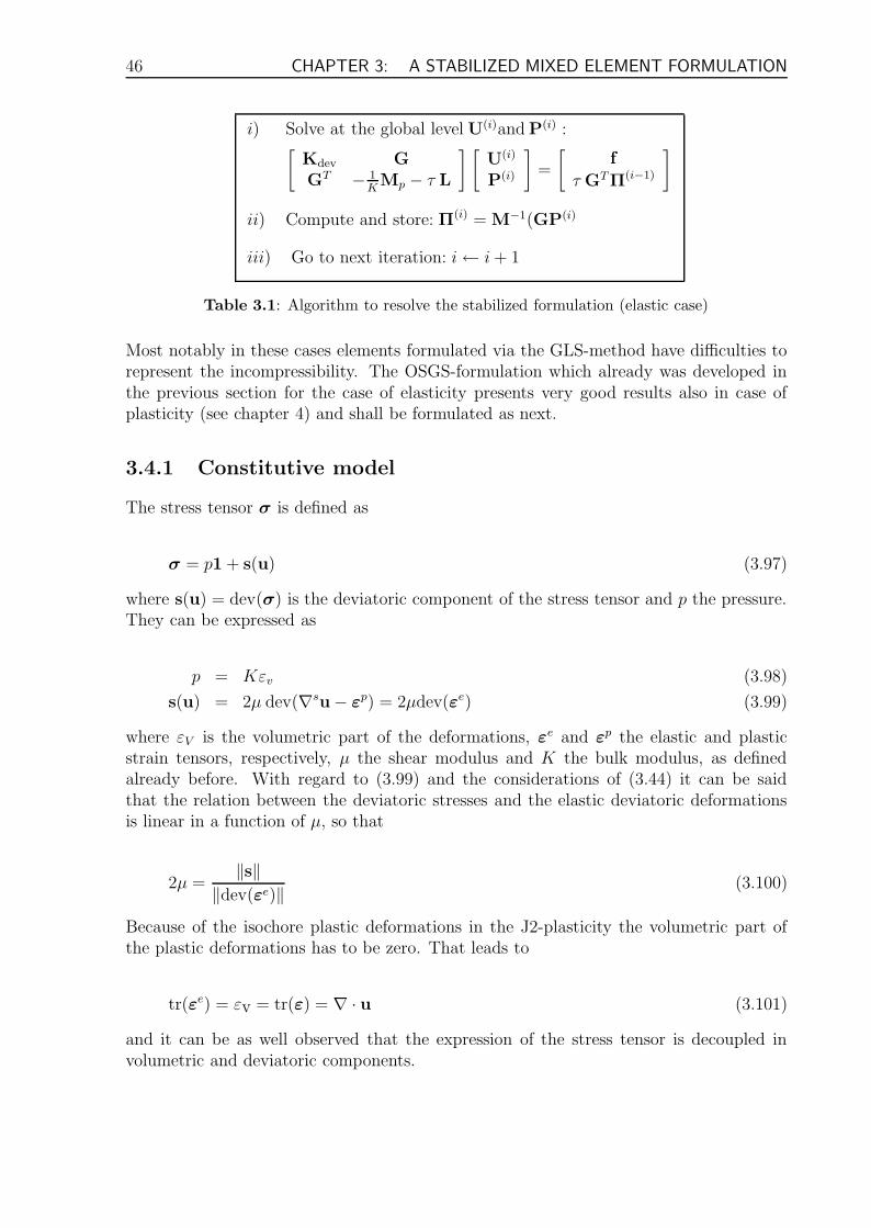
46 CHAPTER 3: A STABILIZED MIXED ELEMENT FORMULATION
i) Solve at the global level U(i)and P(i) :[
Kdev GGT − 1
KMp − τ L
] [U(i)
P(i)
]
=
[f
τ GTΠ(i−1)
]
ii) Compute and store: Π(i) = M−1(GP(i)
iii) Go to next iteration: i← i + 1
Table 3.1: Algorithm to resolve the stabilized formulation (elastic case)
Most notably in these cases elements formulated via the GLS-method have difficulties torepresent the incompressibility. The OSGS-formulation which already was developed inthe previous section for the case of elasticity presents very good results also in case ofplasticity (see chapter 4) and shall be formulated as next.
3.4.1 Constitutive model
The stress tensor σ is defined as
σ = p1 + s(u) (3.97)
where s(u) = dev(σ) is the deviatoric component of the stress tensor and p the pressure.They can be expressed as
p = Kεv (3.98)
s(u) = 2µ dev(∇su− εp) = 2µdev(εe) (3.99)
where εV is the volumetric part of the deformations, εe and ε
p the elastic and plasticstrain tensors, respectively, µ the shear modulus and K the bulk modulus, as definedalready before. With regard to (3.99) and the considerations of (3.44) it can be saidthat the relation between the deviatoric stresses and the elastic deviatoric deformationsis linear in a function of µ, so that
2µ =‖s‖
‖dev(εe)‖(3.100)
Because of the isochore plastic deformations in the J2-plasticity the volumetric part ofthe plastic deformations has to be zero. That leads to
tr(εe) = εv = tr(ε) = ∇ · u (3.101)
and it can be as well observed that the expression of the stress tensor is decoupled involumetric and deviatoric components.
3.4 Formulation in the plastic case 47
3.4.2 Formulation in the continuum
3.4.2.1 The strong form
The problem of the strong form is defined by the previous constitutive equations (3.98)and (3.99), the equilibrium condition and the boundary conditions. Additionally, forthe mixed formulation has to be fulfilled the condition for the volumetric deformation in(2.15). Altogether can be expressed once again as:
Given are the prescribed values of the external forces t : ∂tΩ→ RND, the displacementson the boundary ∂uΩ and the body forces b : Ω → RND; find then U := [u, p]T ∈ W =V × Q, so that
L(U) = F (3.102)
where
L(U) =
[−∇p−∇ · s(u)− 1
Kp +∇ · u
]
(3.103)
F =
[f0
]
(3.104)
and additionally the boundary conditions:
u = 0 in ∂Ωu (3.105)
σ · n = t in ∂Ωt (3.106)
where the expression of the stress tensor σ has been replaced by the dependency of u andp.
3.4.2.2 The weak form
The associated weak form can be written in the compact notation as:
Find U := [u p]T ∈ W = V × Q, so that
R(U,V) = 0 , ∀W ∈ W (3.107)
with
R(U,V) =
[〈∇sv, s〉+ 〈∇ · v, p〉 − 〈v, f〉 − 〈v, t〉∂tΩ
〈q,∇ · u〉 − 〈q, 1K
p〉
]
(3.108)
48 CHAPTER 3: A STABILIZED MIXED ELEMENT FORMULATION
The vectors U := [u p]T ∈ W and V := [v q]T ∈ W are the vector of the unknowns andits respective variation and W is the space of the admissible functions.The spaces V and Q are the space of the displacements and the space of the pressure,respectively. In the continuum they are defined as
V =v |v ∈ H1(Ω) , v = 0 in ∂Ωu
(3.109)
Q =
q | q ∈ L2(Ω) ,
∫
Ω
q dΩ = 0
(3.110)
3.4.3 Extension to multiscales
The solution of the unknowns are approximated by
U = Uh + U (3.111)
V = Vh + V (3.112)
The space in which the solution U is defined will be split as well in two parts as W =Wh ⊕ V so that Uh ∈ Wh and U ∈ W . Furthermore, by following a similar proceedingas in the elastic case, demonstrated in details in the previous chapter 3.3, the problem inthe continuum (3.107) transforms into:Find Uh ∈ Wh and U ∈ W , so that
R(U,Vh) = R(Uh + U,Vh) = 0 , ∀Vh ∈ Vh,0 (3.113)
R(U, V) = R(Uh + U, V) = 0 , ∀ V ∈ V (3.114)
It can be observed that equation (3.113) contains the equilibrium condition and the condi-tion for the volumetric deformations defined in the finite element spaceWh. The equation(3.114) is defined in the space W which will be used to obtain an approximation of thesub-grid scales.Preceding to the development of the method, it shall be introduced a consideration onthe deviatoric stresses, taking into account that the effect of the sub-grid scales is ofthe order u ∼ O(h2); see also [9]. Agreeing to this, the deviatoric components of thestresses s(u) can be approximated via a Taylor series of the first order outside of uh asf(x0 +∆x) = f(x0)+f ′(x)|x=x0
∆x, without attention to the terms of quadratic or higherorder and coming after all to
s(uh + u) = sh(uh) + Cs|u=uh: ∇su +O(u)2 (3.115)
where Cs|u=uhis the deviatoric part of the tangential constitutive tensor evaluated in
u = uh. This tensor relates the deviatoric stresses with the total stains. The tensorialproduct Cs|u=uh
: ∇su represents an increment of deviatoric stresses for the effect of the
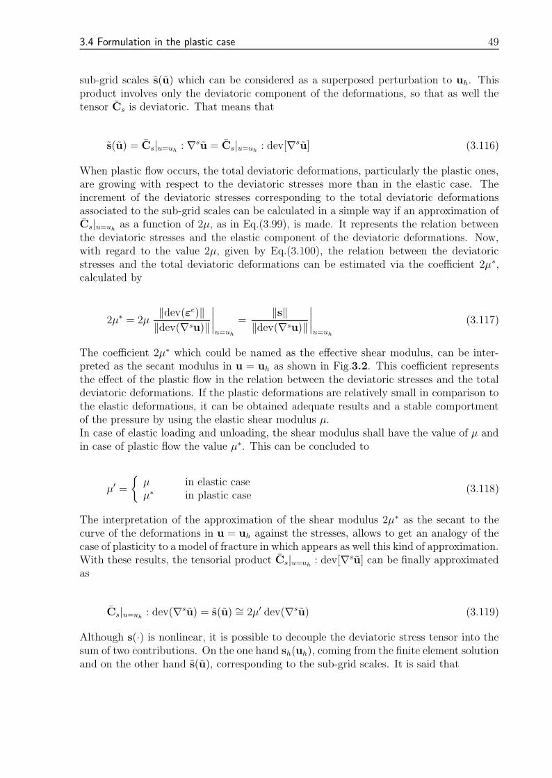
3.4 Formulation in the plastic case 49
sub-grid scales s(u) which can be considered as a superposed perturbation to uh. Thisproduct involves only the deviatoric component of the deformations, so that as well thetensor Cs is deviatoric. That means that
s(u) = Cs|u=uh: ∇su = Cs|u=uh
: dev[∇su] (3.116)
When plastic flow occurs, the total deviatoric deformations, particularly the plastic ones,are growing with respect to the deviatoric stresses more than in the elastic case. Theincrement of the deviatoric stresses corresponding to the total deviatoric deformationsassociated to the sub-grid scales can be calculated in a simple way if an approximation ofCs|u=uh
as a function of 2µ, as in Eq.(3.99), is made. It represents the relation betweenthe deviatoric stresses and the elastic component of the deviatoric deformations. Now,with regard to the value 2µ, given by Eq.(3.100), the relation between the deviatoricstresses and the total deviatoric deformations can be estimated via the coefficient 2µ∗,calculated by
2µ∗ = 2µ‖dev(εe)‖
‖dev(∇su)‖
∣∣∣∣u=uh
=‖s‖
‖dev(∇su)‖
∣∣∣∣u=uh
(3.117)
The coefficient 2µ∗ which could be named as the effective shear modulus, can be inter-preted as the secant modulus in u = uh as shown in Fig.3.2. This coefficient representsthe effect of the plastic flow in the relation between the deviatoric stresses and the totaldeviatoric deformations. If the plastic deformations are relatively small in comparison tothe elastic deformations, it can be obtained adequate results and a stable comportmentof the pressure by using the elastic shear modulus µ.In case of elastic loading and unloading, the shear modulus shall have the value of µ andin case of plastic flow the value µ∗. This can be concluded to
µ′ =
µ in elastic caseµ∗ in plastic case
(3.118)
The interpretation of the approximation of the shear modulus 2µ∗ as the secant to thecurve of the deformations in u = uh against the stresses, allows to get an analogy of thecase of plasticity to a model of fracture in which appears as well this kind of approximation.With these results, the tensorial product Cs|u=uh
: dev[∇su] can be finally approximatedas
Cs|u=uh: dev(∇su) = s(u) ∼= 2µ′ dev(∇su) (3.119)
Although s(·) is nonlinear, it is possible to decouple the deviatoric stress tensor into thesum of two contributions. On the one hand sh(uh), coming from the finite element solutionand on the other hand s(u), corresponding to the sub-grid scales. It is said that
50 CHAPTER 3: A STABILIZED MIXED ELEMENT FORMULATION
Figure 3.2: Graph of the deviatoric stresses against the deviatoric deformations in case ofJ2-plasticity
s(uh + u) ∼= sh(uh) + s(u) (3.120)
According to this and taking into account that the divergence operator is linear, theexpression (3.113) can be separated into
R(Uh,Vh) + R(U,Vh) = 0 , ∀Vh ∈ Wh (3.121)
where R(Uh,Vh) and R(U,Vh) are respectively
R(Uh,Vh) =
[〈∇svh, sh〉Ω′ + 〈∇ · vh, ph〉Ω′ − l(vh)
〈qh,∇ · uh −1K
ph〉Ω′
]
(3.122)
R(U,Vh) =
[〈∇svh, 2µ
′ dev(∇su)〉Ω′
〈qh,∇ · u〉Ω′
]
(3.123)
The second term represents the effect of the sub-grid scales in the finite element solution.The integration by parts of this term, with the aim to reduce the order of derivation ofu, leads to
R(U,Vh) =
[−〈u,∇ · [2µ′ dev(∇svh)〉Ω′
−〈u,∇qh〉Ω′
]
(3.124)
If the additive decomposition of the stress tensor (3.120) is used in Eq.(3.114) this equationcan be rewritten as
3.4 Formulation in the plastic case 51
R(U, V) =
[〈v,∇ · sh〉Ω′ + 〈v,∇ · s〉Ω′ + 〈v,∇ph〉Ω′ + 〈v,b〉Ω′
0
]
= 0 (3.125)
It can be observed that there is no equation associated to the variations of the pressurebecause of considering only the sub-grid scales for the displacements. With the decouplingof the vector U in its parts Uh and U we get
R(Uh, V) + R(U, V) = 0 , ∀ V ∈ W (3.126)
which leads to
−〈v,∇ · [2µ′ dev(∇su)]〉Ω′ = 〈v,∇ · sh +∇ph + b〉Ω′ (3.127)
This is the relation between the sub-grid scale and the residuum of the momentum equa-tion Rh = ∇·sh+∇ph + f which is similar to the previous section in Eq.(3.78). Accordingto the adopted considerations in section 3.2.2, it will be chosen the space of orthogonalsub-grid scales W = W⊥
h and with (3.127) the sub-grid scale u can be approximated inevery element as
u = τe P⊥
h (Rh) ∈ W⊥
h (3.128)
where τe is the stabilization parameter and P⊥h (·) represents the projection on the space
W⊥h . The stabilization parameter in linear elements will be calculated by
τe =ch2
2µ′(3.129)
where µ′ accounts for the effect of plastic flow in the deviatoric deformations which ingeneral is calculated in every integration point. In the case of linear triangular elementswith only one integration point per element this value is the only one in each element. Themain robustness of the proposed elements, stabilized by the OSGS-method, make themless sensible to the simplifications considered to the approximation of the stabilizationparameter in comparison to the stabilized elements via others techniques, like the GLS-method used in [15].As seen before, u is the projection of the residuum Rh on the orthogonal space of thefinite element space multiplied by the stabilization parameter. Taking into account thatthe second derivatives of the linear functions of the finite elements are zero and thatP⊥
h (f) = 0, similar to the considerations in the section 3.3.3, we get
u = τe (∇ph − Ph(∇ph)) (3.130)
52 CHAPTER 3: A STABILIZED MIXED ELEMENT FORMULATION
If this approximation is inserted into Eq.(3.125)and it is considered that 〈u,∇ ·(2µ′dev[∇svh])〉Ωe ≡ 0 for linear elements, Eq.(3.124) can be rewritten as
R(U,Vh) =
[0
−∑nelm
e=1 τe〈∇qh,∇ph −Πh〉Ωe
]
(3.131)
where Πh = Ph(∇ph) is the projection of the pressure gradient on the finite element spaceWh.Finally, the proposed stabilized version to resolve the incompressible elasto-plastic prob-lem via linear triangular or tetrahedral elements is defined as:Find [uh, ph, Πh]
T ∈ Vh ×Qh × Vh so that
〈∇svh, sh〉+ 〈∇ · vh, ph〉 − l(vh) = 0 , ∀ vh ∈ Vh (3.132)
〈qh,∇ · uh −1
Kph〉 −
nelm∑
e=1
τe〈∇qh,∇ph −Πh〉Ωe= 0 , ∀ qh ∈ Q (3.133)
〈∇ph, ηh〉 − 〈Πh, ηh〉 = 0 , ∀ ηh ∈ Vh (3.134)
It can be observed that in the proposed formulation the stabilization term effects only onthe equation of the volumetric deformation.According to the adopted considerations in all developed equations appears the total valueof the sub-grid scale instead of the incremental one. For example in the equation (3.127)from which is obtained the approximation of u.
3.4.4 Implementation aspects
The plastic problem implies the nonlinearity of the equation system and consequently thesolution of the equations (3.132)-(3.134) are executed via incremental-iterative procedures.In this scope diverse alternatives to calculate the projection Π are possible. According tothe presented considerations in the section 3.3, the basic strategy consists in decouplingthe projection Π and resolving the mixed system as from now several possibilities exist tobuild up the calculation algorithm. The adopted strategy in this work consists in resolvingsimultaneous the equations of the momentum balance and the volumetric deformationsin the time step t = tn+1. To find the equilibrium in the iterations, the value of theprojection of the pressure gradient Πh is used in the time step t = tn. The value of theprojection of the pressure gradient Πn
h is evaluated on the basis of the converged value ofthe pressure gradient of the previous time step ∇pn
h as
(∇pnh, ηh)− (Πn
h, ηh) = 0 (3.135)
This equation transforms in a trivial system if the lumped mass matrix is used. With thisvalue of Πn
h, the equations of the system which are resolved in the time step n + 1 are
3.4 Formulation in the plastic case 53
〈∇svh, sh(un+1,ih )〉+ 〈∇ · vh, p
n+1,ih 〉 − ln+1(wh) = 0 (3.136)
〈qh,∇ · un+1,ih −
1
Kpn+1,i
h 〉 −
nelm∑
e=1
τe〈∇qh,∇pn+1,ih −Πn
h〉Ωe= 0 (3.137)
In each time step nonlinear equations has to be calculated. This system can be resolved,for example, by applying the Newton-Raphson method. The residuals corresponding tothese equations in the iteration i can be expressed as
rn+1,i1 = 〈∇svh, sh(u
n+1,ih 〉+ 〈∇ · vh, p
n+1,ih 〉 − ln+1(vh) (3.138)
rn+1,i2 = 〈qh,∇ · u
n+1,ih 〉 −
nelm∑
e=1
τe〈∇qh,∇pn+1,ih −Πn
h〉Ωe(3.139)
In each iteration shall be resolved the linear system
a(∆un+1,i+1
h ,vh
)+ 〈∇ · vh, ∆pn+1,i+1
h 〉 = −rn+1,i1 (3.140)
〈qh,∇ ·∆un+1,i+1h −
1
K∆pn+1,i+1
h 〉 −
nelm∑
e=1
τe〈∇qh,∇∆pn+1,i+1h 〉Ωe
= −rn+1,i2 (3.141)
The algorithm to resolve the elasto-plastic problem of the infinitesimals deformations isshown in Tab.3.2. Kdev is the matrix corresponding to the term a(∆un+1,i+1
h ,vh), whosesub-matrix on the element level is
[KAB
dev
]e=
∫
Ωe
(BA)T DBB dΩ (3.142)
where D is the matrix of the deviatoric component of the tangential constitutive tensor.Furthermore, the matrices G, L, Mp and M are defined in the same way as in section3.3 like the vector of the nodal unknowns [U, P]T , too. The residuals R1 and R2 are thevectors associated to the residuals rn+1,i
1 and rn+1,i2 . These are respectively
R1 = f int1 − f ext
1 (3.143)
R2 = f int2 (3.144)
with the internal and external forces defined as:
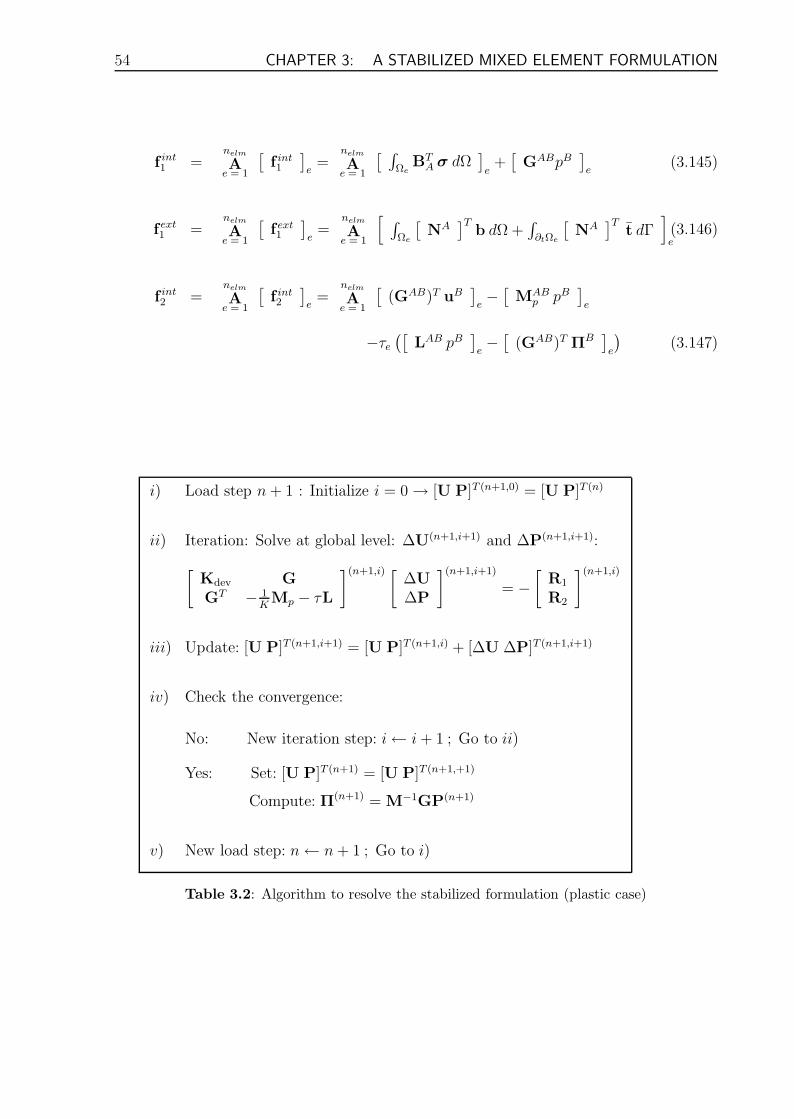
54 CHAPTER 3: A STABILIZED MIXED ELEMENT FORMULATION
f int1 =
nelm
Ae = 1
[f int1
]
e=
nelm
Ae = 1
[ ∫
ΩeBT
A σ dΩ]
e+[
GABpB]
e(3.145)
f ext1 =
nelm
Ae = 1
[f ext1
]
e=
nelm
Ae = 1
[∫
Ωe
[NA
]Tb dΩ +
∫
∂tΩe
[NA
]Tt dΓ
]
e(3.146)
f int2 =
nelm
Ae = 1
[f int2
]
e=
nelm
Ae = 1
[(GAB)T uB
]
e−[
MABp pB
]
e
−τe
([LAB pB
]
e−[
(GAB)T ΠB]
e
)(3.147)
i) Load step n + 1 : Initialize i = 0→ [U P]T (n+1,0) = [U P]T (n)
ii) Iteration: Solve at global level: ∆U(n+1,i+1) and ∆P(n+1,i+1):
[Kdev GGT − 1
KMp − τL
](n+1,i) [∆U∆P
](n+1,i+1)
= −
[R1
R2
](n+1,i)
iii) Update: [U P]T (n+1,i+1) = [U P]T (n+1,i) + [∆U ∆P]T (n+1,i+1)
iv) Check the convergence:
No: New iteration step: i← i + 1 ; Go to ii)
Yes: Set: [U P]T (n+1) = [U P]T (n+1,+1)
Compute: Π(n+1) = M−1GP(n+1)
v) New load step: n← n + 1 ; Go to i)
Table 3.2: Algorithm to resolve the stabilized formulation (plastic case)
Chapter 4
Numerical Results
The efficiency of the proposed formulation can be shown in a series of numerical tests. Thetriangular elements, named as T1P1 for their linear displacement and pressure interpola-tion, shall be compared in diverse examples to other finite element formulations like thesimple linear triangular element without pressure interpolation P1, the simple quadrilat-eral element Q1, the enhanced assumed strain element Q1E4, the improved quadrilateralwith continuous pressure interpolations Q1P0 and a tetrahedral mixed element withoutany stabilization formulation here signified by (P1P1). In the examples are considered aswell the condition of incompressibility as the elasto-plastic comportment simulated by theJ2-plasticity. Most of these examples were calculated by the finite element programme”COupled MEchanical and Thermal analysis (COMET)” and the pre- and postprocessinghas been done by the programme ”GiD”.The examples which will be treated are the patch test, a forced cotter, the Cook’s mem-brane and finally a 2D-block under a displacement load.The patch test is a basic test for the validation of the elements. The problem of the cotterleads to a comparison between the elements mentioned above. The cavity flow problemis a typical problem for mixed finite element methods and gives an example for the verygood comportment of the developed element against the improved elements (EAS andQ1P0). In the problems of elasto-plasticity, like in the problem of the Cook’s membraneand the 2D-block, will be demonstrated the very good results of the proposed elementin spite of its simplifying considerations in case of plasticity against the other mentionedelements.
4.1 Problems in case of elasticity
4.1.1 The patch test
The patch test is the most important prove the finite element methods particularly forintroducing new formulations. The test, first introduced in [13], bases on rational physicsand proves if a patch of elements, subjected to constant deformations, has the capacityto reproduce the exact comportment of the material and returns the according stresses.
55
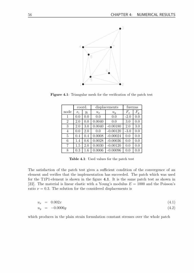
56 CHAPTER 4: NUMERICAL RESULTS
Figure 4.1: Triangular mesh for the verification of the patch test
coord. displacements fuerzasnode xi yi ux uy Fx Fy
1 0.0 0.0 0.0 0.0 -2.0 0.02 2.0 0.0 0.0040 0.0 3.0 0.03 2.0 3.0 0.0040 -0.00180 2.0 3.04 0.0 2.0 0.0 -0.00120 -3.0 0.05 0.4 0.4 0.0008 -0.00024 0.0 0.06 1.4 0.6 0.0028 -0.00036 0.0 0.07 1.5 2.0 0.0030 -0.00120 0.0 0.08 0.3 1.6 0.0006 -0.00096 0.0 0.0
Table 4.1: Used values for the patch test
The satisfaction of the patch test gives a sufficient condition of the convergence of anelement and verifies that the implementation has succeeded. The patch which was usedfor the T1P1-element is shown in the figure 4.1. It is the same patch test as shown in[22]. The material is linear elastic with a Young’s modulus E = 1000 and the Poisson’sratio ν = 0.3. The solution for the considered displacements is
ux = 0.002x (4.1)
uy = −0.0006y (4.2)
which produces in the plain strain formulation constant stresses over the whole patch
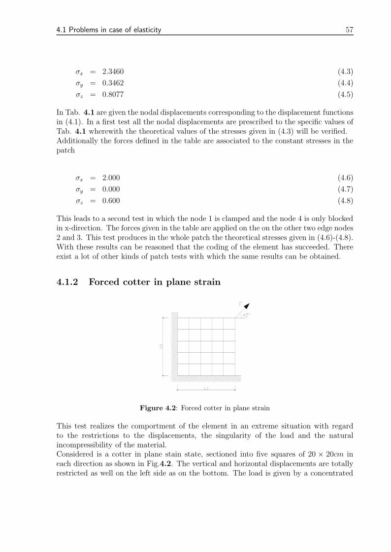
4.1 Problems in case of elasticity 57
σx = 2.3460 (4.3)
σy = 0.3462 (4.4)
σz = 0.8077 (4.5)
In Tab. 4.1 are given the nodal displacements corresponding to the displacement functionsin (4.1). In a first test all the nodal displacements are prescribed to the specific values ofTab. 4.1 wherewith the theoretical values of the stresses given in (4.3) will be verified.Additionally the forces defined in the table are associated to the constant stresses in thepatch
σx = 2.000 (4.6)
σy = 0.000 (4.7)
σz = 0.600 (4.8)
This leads to a second test in which the node 1 is clamped and the node 4 is only blockedin x-direction. The forces given in the table are applied on the on the other two edge nodes2 and 3. This test produces in the whole patch the theoretical stresses given in (4.6)-(4.8).With these results can be reasoned that the coding of the element has succeeded. Thereexist a lot of other kinds of patch tests with which the same results can be obtained.
4.1.2 Forced cotter in plane strain
Figure 4.2: Forced cotter in plane strain
This test realizes the comportment of the element in an extreme situation with regardto the restrictions to the displacements, the singularity of the load and the naturalincompressibility of the material.Considered is a cotter in plane stain state, sectioned into five squares of 20 × 20cm ineach direction as shown in Fig.4.2. The vertical and horizontal displacements are totallyrestricted as well on the left side as on the bottom. The load is given by a concentrated

58 CHAPTER 4: NUMERICAL RESULTS
Standard Quadrilateral (Q1) EAS-Formulation (Q1E4)
Q1P0-Formulation Standard Triangle (P1)
Instable Mixed Element (P1P1) OSGS-Formulation (P1T1)
Figure 4.3: Forced cutter in plane strain: distribution to the pressure
load on the right upper corner of the cotter which has tension component as well to thex-direction as to the y-directions with the value of Fx = Fy = 5 · 106N/m. The materialexhibits a Young’s modulus of E = 2.0 · 105MPa and a Poisson’s ratio of ν = 0.4999,which is nearly almost incompressible. Compared elements formulations are the P1, Q1,P1P1, Q1P0, Q1E4 and the T1P1 as defined above.The resulted distributions of the pressure and the Von Mises stresses are shown in thedeformed geometry of the cotter whereby the increase factor is for each element type thesame. The locking effect of the two standard elements can be noticed in the results inFig.4.3. The extreme stiffness of the elements is confirmed by the very small deformationof the mesh and also by the illustration of the pressure which is completely unphysically.The instable mixed element shows already better displacements but the very inhomoge-neous pressure image reasons to a inaccurate pressure calculation. The pressure values ofthe Q1P0-element and the EAS-element are very low but their deformation figure showsa slight irregularity in the shape, in case of the Q1P0-element more than in case of theEAS-element. This is caused by the hourglass modes which can occur if the stabilizationof the element formulation is accomplished by the static condensation of the additionalvariable, so in case of the Q1P0-element the volumetric deformations are constant in the
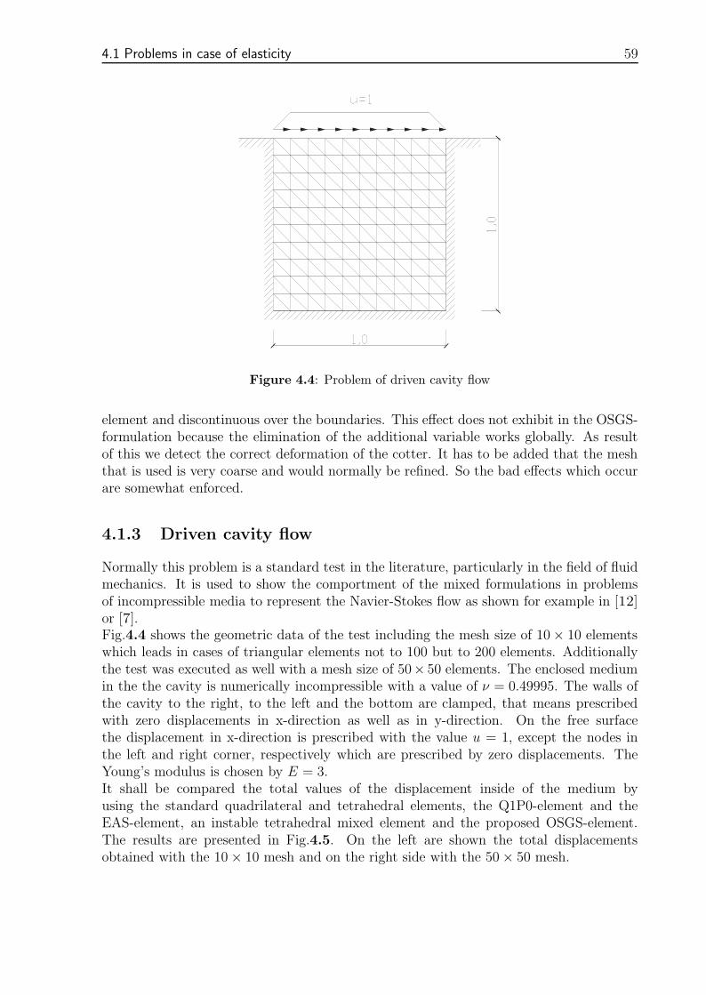
4.1 Problems in case of elasticity 59
Figure 4.4: Problem of driven cavity flow
element and discontinuous over the boundaries. This effect does not exhibit in the OSGS-formulation because the elimination of the additional variable works globally. As resultof this we detect the correct deformation of the cotter. It has to be added that the meshthat is used is very coarse and would normally be refined. So the bad effects which occurare somewhat enforced.
4.1.3 Driven cavity flow
Normally this problem is a standard test in the literature, particularly in the field of fluidmechanics. It is used to show the comportment of the mixed formulations in problemsof incompressible media to represent the Navier-Stokes flow as shown for example in [12]or [7].Fig.4.4 shows the geometric data of the test including the mesh size of 10× 10 elementswhich leads in cases of triangular elements not to 100 but to 200 elements. Additionallythe test was executed as well with a mesh size of 50× 50 elements. The enclosed mediumin the the cavity is numerically incompressible with a value of ν = 0.49995. The walls ofthe cavity to the right, to the left and the bottom are clamped, that means prescribedwith zero displacements in x-direction as well as in y-direction. On the free surfacethe displacement in x-direction is prescribed with the value u = 1, except the nodes inthe left and right corner, respectively which are prescribed by zero displacements. TheYoung’s modulus is chosen by E = 3.It shall be compared the total values of the displacement inside of the medium byusing the standard quadrilateral and tetrahedral elements, the Q1P0-element and theEAS-element, an instable tetrahedral mixed element and the proposed OSGS-element.The results are presented in Fig.4.5. On the left are shown the total displacementsobtained with the 10× 10 mesh and on the right side with the 50× 50 mesh.
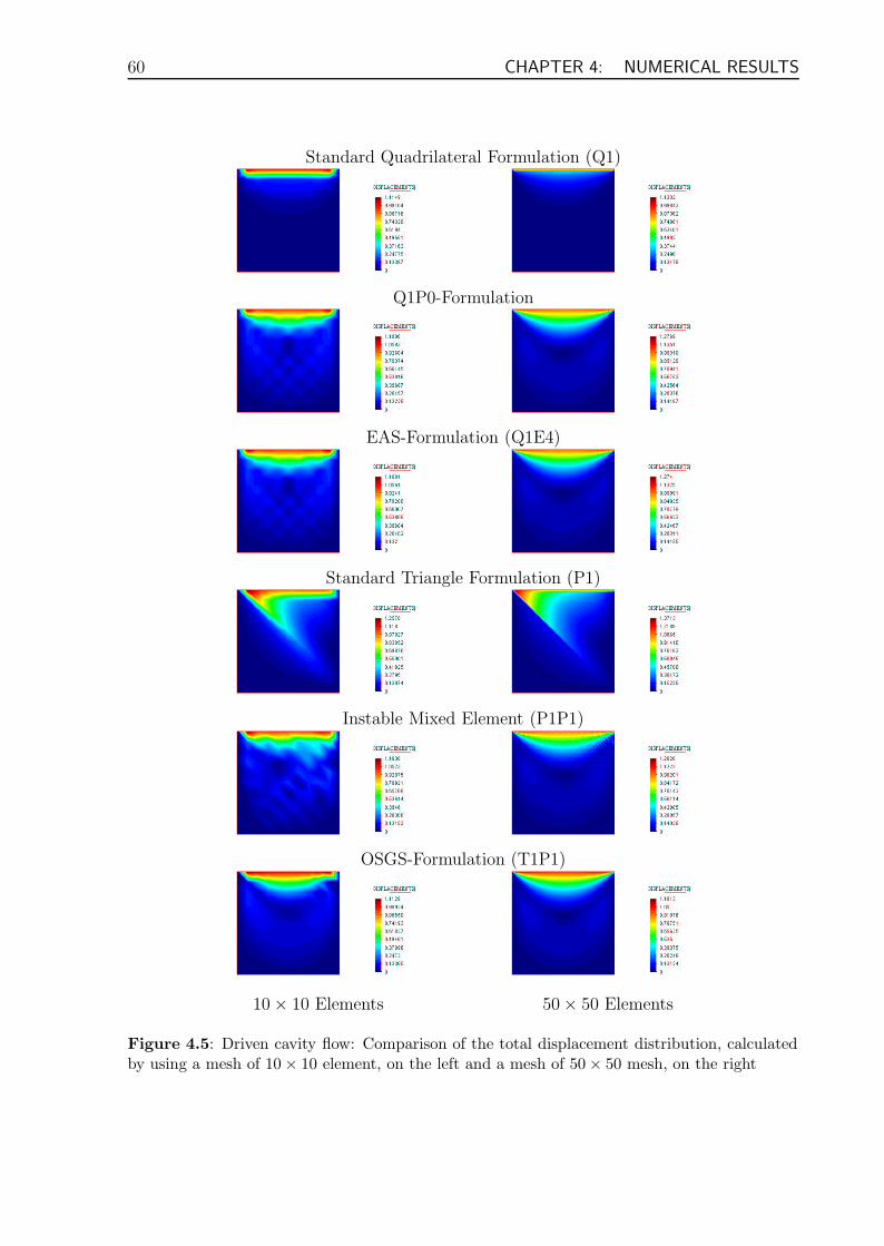
60 CHAPTER 4: NUMERICAL RESULTS
Standard Quadrilateral Formulation (Q1)
Q1P0-Formulation
EAS-Formulation (Q1E4)
Standard Triangle Formulation (P1)
Instable Mixed Element (P1P1)
OSGS-Formulation (T1P1)
10× 10 Elements 50× 50 Elements
Figure 4.5: Driven cavity flow: Comparison of the total displacement distribution, calculatedby using a mesh of 10× 10 element, on the left and a mesh of 50× 50 mesh, on the right
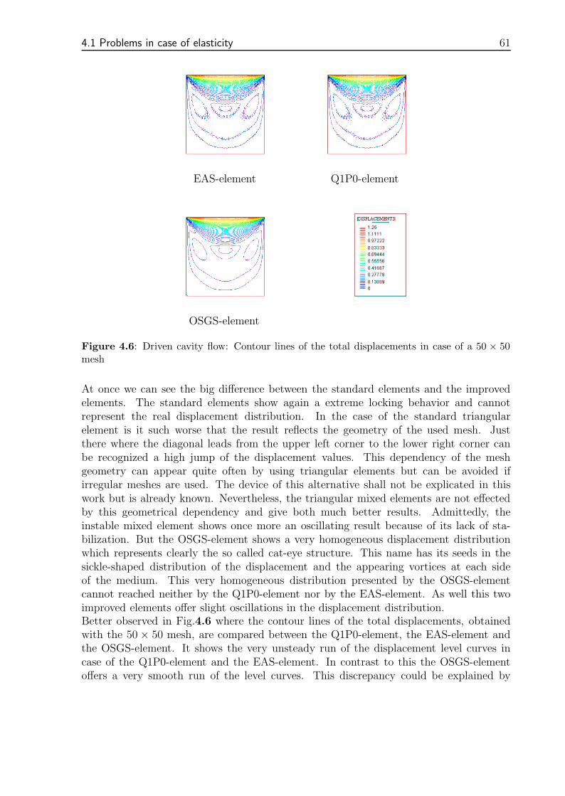
4.1 Problems in case of elasticity 61
EAS-element Q1P0-element
OSGS-element
Figure 4.6: Driven cavity flow: Contour lines of the total displacements in case of a 50 × 50mesh
At once we can see the big difference between the standard elements and the improvedelements. The standard elements show again a extreme locking behavior and cannotrepresent the real displacement distribution. In the case of the standard triangularelement is it such worse that the result reflects the geometry of the used mesh. Justthere where the diagonal leads from the upper left corner to the lower right corner canbe recognized a high jump of the displacement values. This dependency of the meshgeometry can appear quite often by using triangular elements but can be avoided ifirregular meshes are used. The device of this alternative shall not be explicated in thiswork but is already known. Nevertheless, the triangular mixed elements are not effectedby this geometrical dependency and give both much better results. Admittedly, theinstable mixed element shows once more an oscillating result because of its lack of sta-bilization. But the OSGS-element shows a very homogeneous displacement distributionwhich represents clearly the so called cat-eye structure. This name has its seeds in thesickle-shaped distribution of the displacement and the appearing vortices at each sideof the medium. This very homogeneous distribution presented by the OSGS-elementcannot reached neither by the Q1P0-element nor by the EAS-element. As well this twoimproved elements offer slight oscillations in the displacement distribution.Better observed in Fig.4.6 where the contour lines of the total displacements, obtainedwith the 50× 50 mesh, are compared between the Q1P0-element, the EAS-element andthe OSGS-element. It shows the very unsteady run of the displacement level curves incase of the Q1P0-element and the EAS-element. In contrast to this the OSGS-elementoffers a very smooth run of the level curves. This discrepancy could be explained by
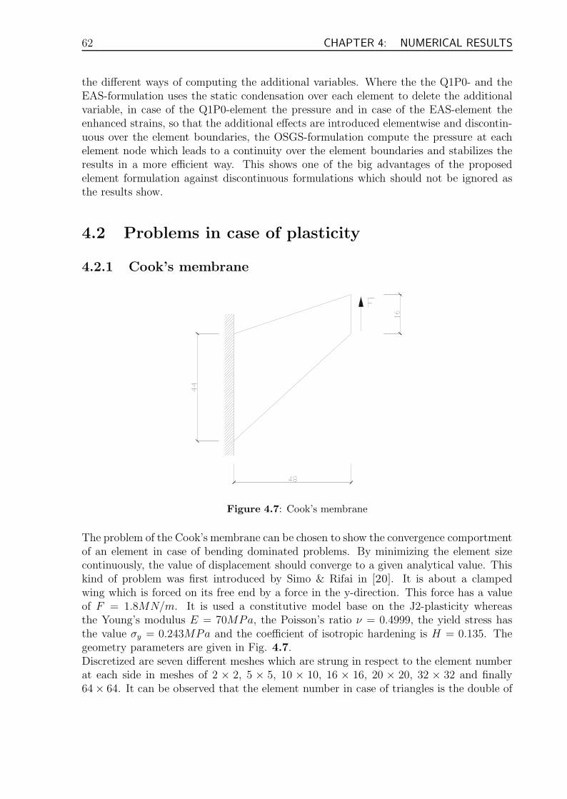
62 CHAPTER 4: NUMERICAL RESULTS
the different ways of computing the additional variables. Where the the Q1P0- and theEAS-formulation uses the static condensation over each element to delete the additionalvariable, in case of the Q1P0-element the pressure and in case of the EAS-element theenhanced strains, so that the additional effects are introduced elementwise and discontin-uous over the element boundaries, the OSGS-formulation compute the pressure at eachelement node which leads to a continuity over the element boundaries and stabilizes theresults in a more efficient way. This shows one of the big advantages of the proposedelement formulation against discontinuous formulations which should not be ignored asthe results show.
4.2 Problems in case of plasticity
4.2.1 Cook’s membrane
Figure 4.7: Cook’s membrane
The problem of the Cook’s membrane can be chosen to show the convergence comportmentof an element in case of bending dominated problems. By minimizing the element sizecontinuously, the value of displacement should converge to a given analytical value. Thiskind of problem was first introduced by Simo & Rifai in [20]. It is about a clampedwing which is forced on its free end by a force in the y-direction. This force has a valueof F = 1.8MN/m. It is used a constitutive model base on the J2-plasticity whereasthe Young’s modulus E = 70MPa, the Poisson’s ratio ν = 0.4999, the yield stress hasthe value σy = 0.243MPa and the coefficient of isotropic hardening is H = 0.135. Thegeometry parameters are given in Fig. 4.7.Discretized are seven different meshes which are strung in respect to the element numberat each side in meshes of 2 × 2, 5 × 5, 10 × 10, 16 × 16, 20 × 20, 32 × 32 and finally64× 64. It can be observed that the element number in case of triangles is the double of
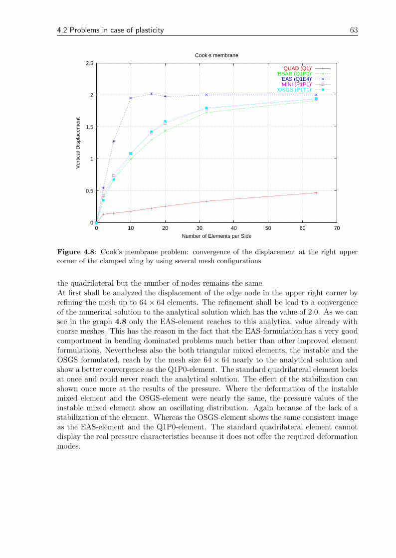
4.2 Problems in case of plasticity 63
0
0.5
1
1.5
2
2.5
0 10 20 30 40 50 60 70
Ver
tical
Dis
plac
emen
t
Number of Elements per Side
Cook·s membrane
’QUAD (Q1)’’BBAR (Q1P0)’
’EAS (Q1E4)’’MINI (P1P1)’
’OSGS (P1T1)’
Figure 4.8: Cook’s membrane problem: convergence of the displacement at the right uppercorner of the clamped wing by using several mesh configurations
the quadrilateral but the number of nodes remains the same.At first shall be analyzed the displacement of the edge node in the upper right corner byrefining the mesh up to 64× 64 elements. The refinement shall be lead to a convergenceof the numerical solution to the analytical solution which has the value of 2.0. As we cansee in the graph 4.8 only the EAS-element reaches to this analytical value already withcoarse meshes. This has the reason in the fact that the EAS-formulation has a very goodcomportment in bending dominated problems much better than other improved elementformulations. Nevertheless also the both triangular mixed elements, the instable and theOSGS formulated, reach by the mesh size 64 × 64 nearly to the analytical solution andshow a better convergence as the Q1P0-element. The standard quadrilateral element locksat once and could never reach the analytical solution. The effect of the stabilization canshown once more at the results of the pressure. Where the deformation of the instablemixed element and the OSGS-element were nearly the same, the pressure values of theinstable mixed element show an oscillating distribution. Again because of the lack of astabilization of the element. Whereas the OSGS-element shows the same consistent imageas the EAS-element and the Q1P0-element. The standard quadrilateral element cannotdisplay the real pressure characteristics because it does not offer the required deformationmodes.
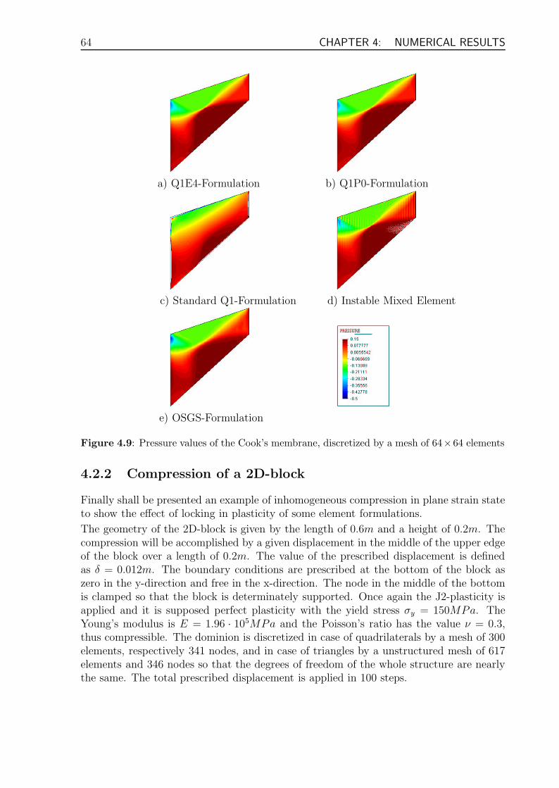
64 CHAPTER 4: NUMERICAL RESULTS
a) Q1E4-Formulation b) Q1P0-Formulation
c) Standard Q1-Formulation d) Instable Mixed Element
e) OSGS-Formulation
Figure 4.9: Pressure values of the Cook’s membrane, discretized by a mesh of 64×64 elements
4.2.2 Compression of a 2D-block
Finally shall be presented an example of inhomogeneous compression in plane strain stateto show the effect of locking in plasticity of some element formulations.
The geometry of the 2D-block is given by the length of 0.6m and a height of 0.2m. Thecompression will be accomplished by a given displacement in the middle of the upper edgeof the block over a length of 0.2m. The value of the prescribed displacement is definedas δ = 0.012m. The boundary conditions are prescribed at the bottom of the block aszero in the y-direction and free in the x-direction. The node in the middle of the bottomis clamped so that the block is determinately supported. Once again the J2-plasticity isapplied and it is supposed perfect plasticity with the yield stress σy = 150MPa. TheYoung’s modulus is E = 1.96 · 105MPa and the Poisson’s ratio has the value ν = 0.3,thus compressible. The dominion is discretized in case of quadrilaterals by a mesh of 300elements, respectively 341 nodes, and in case of triangles by a unstructured mesh of 617elements and 346 nodes so that the degrees of freedom of the whole structure are nearlythe same. The total prescribed displacement is applied in 100 steps.
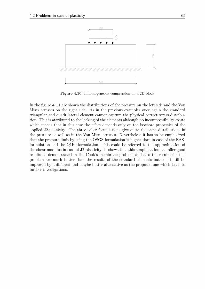
4.2 Problems in case of plasticity 65
Figure 4.10: Inhomogeneous compression on a 2D-block
In the figure 4.11 are shown the distributions of the pressure on the left side and the VonMises stresses on the right side. As in the previous examples once again the standardtriangular and quadrilateral element cannot capture the physical correct stress distribu-tion. This is attributed to the locking of the elements although no incompressibility existswhich means that in this case the effect depends only on the isochore properties of theapplied J2-plasticity. The three other formulations give quite the same distributions inthe pressure as well as in the Von Mises stresses. Nevertheless it has to be emphasizedthat the pressure limit by using the OSGS-formulation is higher than in case of the EAS-formulation and the Q1P0-formulation. This could be referred to the approximation ofthe shear modulus in case of J2-plasticity. It shows that this simplification can offer goodresults as demonstrated in the Cook’s membrane problem and also the results for thisproblem are much better than the results of the standard elements but could still beimproved by a different and maybe better alternative as the proposed one which leads tofurther investigations.
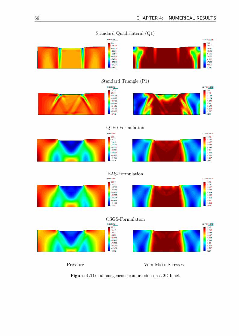
66 CHAPTER 4: NUMERICAL RESULTS
Standard Quadrilateral (Q1)
Standard Triangle (P1)
Q1P0-Formulation
EAS-Formulation
OSGS-Formulation
Pressure Vom Mises Stresses
Figure 4.11: Inhomogeneous compression on a 2D-block

Chapter 5
Conclusion
5.1 Summary
The demonstrated object in this work was the development of an efficient low-order ele-ment formulation with the capacity to represent the problem of incompressibility in solidmechanics. The standard elements of low order unite various requirements for the utilityin practical applications but present locking effects in the case of incompressibility. Thealternative in view of this difficulty can be the mixed finite element formulation. Thestability of the mixed elements depends on the compatibility between the involved in-terpolation fields. The mathematic condition that expresses this restriction is known asthe stability condition of Ladyzhenskaya-Babuska-Brezzi or LBB-condition. The mixedelements with linear displacement and pressure interpolations do not satisfy this con-dition and therefore present stabilization problems which are manifested in the lack ofthe control over the pressure. This means that the feasibility of these mixed elementsrequire the application of a stabilization method. The stabilization method used in thiswork bases on the concept of the sub-grid scale approach, particularly the method oforthogonal sub-grid scales (OSGS). From the point of view of the method, the numericalinstabilities of certain formulations have the reason in the fact that the effects of the un-resolved components of the solution, named as sub-grid scales, are not taken into accountin the balance equations. The concept of the orthogonal sub-grid scales proposes thatthe orthogonal space to the finite element space is the natural space to search for thesub-grid scales of the solution. The stabilization method circumvents the LBB-conditionand allows to obtain elements with interpolations of the same order for the displacementand the pressure fields.
5.2 Statements
The main conclusions of this work shall be resumed in the following statements:
• An adequate finite element formulation to represent the problem of incompressibil-ity in solid mechanics has been developed, implemented and valuated; in case of
67
68 CHAPTER 5: CONCLUSION
elasticity as well as in case of J2-plasticity.
• The developed elements are mixed elements stabilized by the method of orthogonalsub-grid scales (OSGS) and exhibit linear and continuous interpolations of the dis-placement and the pressure fields. These elements offer low computational cost andshow good comportments against other known element formulations like the EAS-and the Q1P0-element.
• The developed formulation can be applied to triangular as well as to quadrilateralelements. However the linear triangular element is more interesting for the practicalapplication because of its possibility to generate meshes of complexer geometries asused in many industrial problems. This is a great advantage against the quadrilat-eral element formulations as for example the EAS-formulation or the Q1P0-element.
• The proposed element is able to represent the situation of incompressibility in asatisfying way. The condition of incompressibility is obliged in the global form. Incontrast to this in elements like the Q1P0-element this condition is obliged elementwise which can lead in extreme situations to the so called hourglassing, a kind ofeigenmodes that degrade the result of the solution.
5.3 Aspects of future investigation
Following considerations could be made to improve or to expand the application of thedeveloped element formulation:
• The introduction of the sub-grid scale to the pressure in the formulation. The capa-bility of the orthogonal sub-grid scales has been utilized only in the formulation ofthe displacement field and it could be observed that the formulation gives satisfyingresults. Nevertheless, the integration of the sub-grid scales of the pressure couldimprove once more the stabilizing characteristics.
• The study of the influence in case of compressibility to the stabilization parameter.
• Enhancing the developed formulation to the case of finite deformations (already inprogress and partially concluded by the work of M. Cervera and M. Chiumenti butnot mentioned in this work).
• Finding alternatives or improvements for the approximation of the stabilizationparameter τ and the shear modulus µ∗ in case of J2-plasticity.
• Looking for further alternatives for the sub-grid scale approach and comparing themto the presented orthogonal sub-grid scales.
• The study of dynamic problems and their effect on the stabilization method.

5.3 Aspects of future investigation 69
• Developing other applications of the stabilization method in solid mechanics likecoupled thermo-mechanical problems, contact problems, shell formulations, fracturemodels and so on.
()
References
[1]ARNOLD, D. N.; BREZZI, F.; FORTIN, M.: A stable finite element for the Stokesequations, Calculo, Vol. 21, pp. 337-344 (1984)
[2]BAIOCCHI, C.; BREZZI, F.; FRANCA, P. F.: Virtual bubbles and Galerkin-least-squares type methods, Computer Methods in Applied Mechanics and EngineeringVol. 105, pp. 125-141 (1993)
[3]BATHE, K. J.: Finite Elemente Methoden, Springer Verlag, 2. Auflage (2002)
[4]BREZZI, F.; FORTIN, M.: Mixed and Hybrid Finite Element Methods, Springer Verlag(1991)
[5]CHIUMENTI, M.; VALVERDE, Q.; AGELET DE SARACIBAR, C.; CERVERA, M.:A stabilized formulation for incompressible elasticity using linear displacement andpressure interpolations, Computational Methods in Applied Mechanics and Engineer-ing, Vol. 191, pp. 5253-5264 (2002)
[6]CIARLET, P.G.: The Finite Element Method for Elliptic Problems, North Holland,New York (1978)
[7]CODINA, R.: A finite element model for incompressible flow problems, PhD. thesis,Universitat Polytecnica de Catalunya (1992)
[8]CODINA, R.: Stabilization of incompressibility and convection through orthogonalsub-scales in finite element methods, Computer Methods in Applied Mechanics, Vol.190, pp. 1579-1599 (2000)
[9]CODINA, R.: Stabilized finite element approximation of transient incompressible flowsusing orthogonal sub-scales, Computer Methods in Applied Mechanics, Vol. 191, pp.4295-4321 (2002)
[10]CODINA, R.; VASQUEZ, M.; ZIENKIEWICZ, O.: A general algorithm for compress-ible and incompressible flow - part III: The semi-implicit form, International Journalfor Numerical Methods in Fluids, Vol. 27, pp. 13-32 (1998)
[11]HUGHES, T. J. R.; FRANCA, L.; BALESTRA, M.: A new finite element formulationfor computational fluid dynamics: V. Circumventing the Babuska-Brezzi condition: Astable Petrov-Galerkin formulation of the Stokes problem accommodating equal-orderinterpolations, Computer Methods in Applied Mechanics, Vol. 59, pp. 85-99 (1986)
[12]HUGHES, T. J. R.: The Finite Element Method - Linear Static and Dynamic FiniteElement Analysis, Dover Publications Inc. (2000)
70
References 71
[13]IRONS, B.; RAZZAQUE A.: Experiences with the patch test for convergence offinite elements, The Mathematical Foundations of the Finite Element Method withApplications to Partial Differential Equations, pp. 557587, Academic Press, New York(1972)
[14]KASPER, E. P.; TAYLOR, T. L.: A Mixed-Enhanced Strain Method: Linear Prob-lems, UCB/SEMM-97/02 (1997)
[15]KLAAS, O.; MANIATTY, A.; SHEPHARD, M. S.: A stabilized mixed finite elementmethod for finite elasticity formulation for linear displacement and pressure interpola-tions, Computer Methods in Applied Mechanics and Engineering, Vol. 180, pp. 65-79(1999)
[16]MALKUS, D. S.; HUGHES, T. J. R.: Mixed Finite Element Methods - Reduced andSelective Integration Techniques: A Unification of Concepts, Computer Methods inApplied Mechanics and Engineering Vol. 15, pp. 68-81 (1978)
[17]PERCHAT, E.: MINI-Element et factorisations incompletes pour la parallelisationd’un solveur de Stokes 2D - Application au forgeage, These Docteur, L’Ecole NationaleSuperieure des Mines de Paris (2000)
[18]QUECEDO, M.; PASTOR, M.; ZIENKIEWICZ, O. C.: Enhanced linear trianglefor plasticity problems in J2-Solids, Computer Methods in Applied Mechanics andEngineering, Vol. 188, pp. 145-163 (2000)
[19]REESE, S.: Advanced Finite Element Technology, Numerische Mechanik und Simu-lationstechnik, Ruhr University Bochum (2001)
[20]SIMO, J. C.; RIFAI, M. S.: A class of mixed assumed strain methods and the methodof incompatible modes, International Journal for Numerical Methods in Engineering,Vol. 29, pp. 1595-1638 (1990)
[21]VALVERDE GUZMAN, Q. M.: Elementos estabilizados de bajo orden en mecnica deslidos, Tesis Doctoral, Universitat Politcnica de Catalunya (2002)
[22]ZIENKIEWICZ, O. C.; TAYLOR, R. L.: The Finite Element Method - Volume 1,Butterworth Heinemann, 5th edition (1999)